VQ-SGen: A Vector Quantized Stroke Representation for Sketch Generation

Abstract

This paper presents VQ-SGen, a novel algorithm for high-quality sketch generation. Recent approaches have often framed the task as pixel-based generation either as a whole or part-by-part, neglecting the intrinsic and contextual relationships among individual strokes, such as the shape and spatial positioning of both proximal and distant strokes. To overcome these limitations, we propose treating each stroke within a sketch as an entity and introducing a vector-quantized (VQ) stroke representation for fine-grained sketch generation. Our method follows a two-stage framework - in the first stage, we decouple each stroke’s shape and location information to ensure the VQ representation prioritizes stroke shape learning. In the second stage, we feed the precise and compact representation into an auto-decoding Transformer to incorporate stroke semantics, positions, and shapes into the generation process. By utilizing tokenized stroke representation, our approach generates strokes with high fidelity and facilitates novel applications, such as conditional generation and semantic-aware stroke editing. Comprehensive experiments demonstrate our method surpasses existing state-of-the-art techniques, underscoring its effectiveness. The code and model will be made publicly available upon publication.

1 Introduction

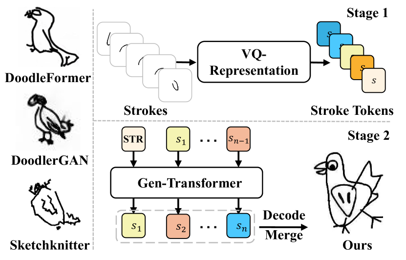
Figure 1: The goal of sketch generation is to generate vivid sketches of a specific category, e.g., the birds from existing methods on the left. We have proposed VQ-SGen, for high-quality sketch generation with a new vector-quantized (VQ) representation and an efficient generator. See one of our results on the right for comparison.

Sketches are an intuitive tool widely used by humans to communicate ideas, convey concepts, and express creativity. Over the past decades, significant research has been conducted on sketch-related tasks, including retrieval [16, 9], semantic segmentation [23, 31], and generation [5, 2, 24]. In this paper, we focus on sketch generation, which offers an automated tool to assist artists and designers in their creative activities. Particularly, Ge et al. [5] introduced the concept of creative sketch generation, aiming to produce more diverse, complex, and aesthetically appealing sketches, thereby placing high demands on the generation capabilities of automatic methods.

Existing methods [5, 2] tackle creative sketch generation by producing pixels either as a whole sketch or as segmented parts, overlooking the inherent and contextual relationships among individual strokes, such as their shapes and relative positions of both nearby and distant strokes. As a consequence, their generated sketches often have blurry local regions, and scattered or isolated strokes (see the head of the bird from DoodleFormer and DoodlerGAN in Fig. 1). A more recent work, SketchKnitter [24], formulated the problem of sketch generation into a stroke points rectification process, where diffusion models are leveraged to rearrange a set of stroke points from an initial chaotic state into coherent forms. However, without the concept of a stroke entity, this method performs poorly when generating complex creative sketches (see the bird in Fig. 1 from SketchKnitter).

To address these limitations, we propose the first stroke-level sketch generation approach that treats each stroke as an independent entity and encodes it using a novel vector-quantized (VQ) representation. This compact, discrete representation enhances the learning process of the generative model by efficiently capturing essential stroke shape variations while minimizing redundancy. Despite the discrete nature of the representation, we observe semantic-aware clustering within the stroke code space, which lays an ideal foundation for the generator to sample new strokes. Furthermore, our bespoke generator incorporates the shape, semantic, and position into its generation process, effectively samples new sketches in the compressed VQ space, and accurately reasons out the structural and semantic relationship between strokes, resulting in sketches that are both appealing and structurally coherent.

Specifically, our method VQ-SGen, adopts a two-stage framework. In the first stage, we decouple the shape and location information of each stroke. This decoupling allows the vector-quantized (VQ) representation to concentrate on capturing stroke shapes, minimizing interference from positional data during the learning process. By prioritizing shape as the primary focus, the model learns a highly compact and informative, shape-oriented representation that preserves the inherent shape features of each stroke while reducing unnecessary redundancy. In the second stage, we employ an autoregressive Transformer to work with our VQ representation. The Transformer progressively integrates the stroke’s semantic (i.e., the category label), shape, and location into the generation process. Through the autoregressive decoding mechanism, the Transformer captures each stroke’s semantic, shape, and context relationship with neighboring strokes, ensuring that the shape and positioning are accurate and harmoniously aligned with its semantic role within the overall composition. As a result, our approach effectively avoids all the artifacts observed in previous methods.

To demonstrate the effectiveness of our method, we have conducted experiments on CreativeSketch [5] datasets. Comprehensive experiments including comparisons and ablation studies show that our method surpasses existing state-of-the-art techniques.

In summary, our main contributions are as follows:

• To the best of our knowledge, we propose the first stroke-level approach, VQ-SGen, for the challenging creative sketch generation task.

• We propose a new vector-quantized (VQ) stroke representation that treats each stroke as an entity, capturing essential shape features compactly and reducing redundancy to serve as the basis for stroke-level sketch generation.

• We propose a bespoke generator, leveraging the shape, semantic, and spatial location together, achieving high-quality generation.

• We extensively evaluated our method, demonstrating superior performance. A further user study shows that VQ-SGen consistently performs favorably against SoTA methods.

2 Related Work

Sketch Representation Learning. Based on the data format of sketches, existing sketch representation learning methods can be broadly divided into three categories: image-based [11, 33, 34], sequence-based [25, 15, 10], and graph-based [28, 22, 30] approaches, each with its own advantages and limitations. Specifically, image-based methods [11, 33, 34] use raster images as input, leveraging absolute coordinates to capture stroke proximity. However, they often struggle to learn structural information and sequential relationships among strokes effectively. Graph-based methods [28, 22, 30] face challenges in capturing detailed structural information within strokes. Sequence-based methods [25, 15, 10] utilize point sequences with relative coordinates, which enhances the encoding of individual stroke structures but makes it difficult to represent inter-stroke proximity and spatial relationships. Given the presented disadvantages, the aforementioned stroke representations are not well suited for the generation task, where the structural and spatial information, as well as the stroke proximity with neighboring strokes, are the core for high-quality and fine-grained generation.

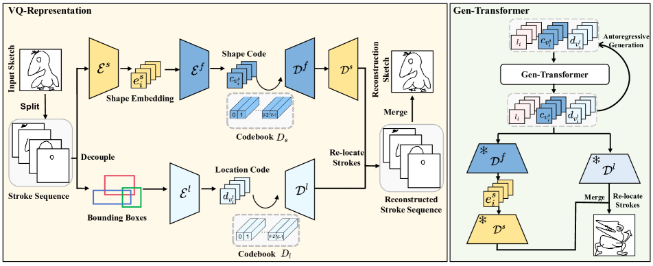
Figure 2: Overview of VQ-SGen. Given an input sketch, it is first divided into a sequence of strokes. In the first stage, we begin by decoupling the shape and location information of each stroke and obtain their discrete representations (Sec. 3.1). In the second stage, we use a decoder-only Gen-Transformer to predict $\left\{\left(\bm{I}_{i},b_{i},l_{i}\right)\right\}$ in an autoregressive manner (Sec. 3.2).

Vector-Quantized VAEs. Learning representations with discrete features has been the focus of many previous works [7, 21, 4], as such representations are a natural choice for complex reasoning, planning, and predictive learning. Although using discrete latent variables in deep learning has been difficult, effective autoregressive models have been created to capture distributions over discrete variables. For instance, StrokeNUWA [18] utilizes VQ-VAE [19] to achieve a better representation of vector graphics, then generates vector graphics through large language models. ShapeFormer [27] presents a new 3D representation called VQDIF and employs an autoregressive model to generate several high-quality completed shapes conditioned on the partial input. Similarly, we propose to learn a VQ representation for rasterized strokes, expecting an improved generation capability powered by the compact representation.

Creative Sketch Generation. Unlike traditional sketch generation tasks [29, 32], creative sketch generation [5] places greater emphasis on producing more imaginative depictions of familiar visual concepts, rather than generating conventional and mundane forms of these concepts. To achieve this goal, DoodlerGAN [5] presents a component-based GAN architecture to incrementally generate each part of a creative sketch image. This approach requires training one GAN model individually for each body part in a supervised way, leading to significant computational overhead. DoodleFormer [2] employs an attention-based architecture for two-stage sketch generation. In the first stage, it captures the overall composition of the rough sketch, while in the second stage, it refines the details to produce the final output. However, this approach tends to focus only on the broad, rough relationships between different parts of the sketch, which can lead to unnatural mixing of strokes from different regions.

3 Method

Sketch and strokes. A standard sketch $\bm{S}$ in our context is composed of a sequence of strokes $\{\bm{s}_{i}\}_{i=1}^{N}$ and their corresponding stroke labels $\{l_{i}\}_{i=1}^{N}$. Note that each stroke is represented as a rasterized image of size $256\times 256$, and each label $l_{i}$ is a one-hot vector in $\mathbb{R}^{C}$. In order to decouple the shape and position of a single stroke, we further process it. Formally, for each rasterized stroke image, we calculate its axis-aligned bounding box and record its center coordinate $(x_{i},y_{i})$. The bounding box size (i.e., the height and width) as well as the center coordinate fully represent the stroke position $b_{i}=(w_{i}/2,h_{i}/2,x_{i},y_{i})$. By factoring out the position (i.e., translating the stroke bounding box to align with the sketch image center), the stroke shape itself is presented as the translated rasterized image $\bm{I}_{i}$. Considering the triplet of shape, position, and semantic of a single stroke, the new format to represent a sketch is $\bm{S}=\{\bm{s}_{i}\}_{i=1}^{N}=\{(\bm{I}_{i},b_{i},l_{i})\}_{i=1}^{N}$.

Sketch generation. Our goal in this paper is to generate a sequence of strokes in the format of the triplet and assemble them based on their shape and position to form the resulting sketch (see Fig. 1). Figure 2 displays an overview of our novel sketch generation method, which is comprised of two main components. Firstly, a decoupled representation learning module encodes a stroke into its vector-quantized representation (Sec. 3.1) that is highly compact and shape-aware. Secondly, a bespoke generator based on the Transformer [20] is designed to generate the stroke label, shape, and location sequentially, achieving a fine-grained control with high-fidelity resulting sketches. In the following, we elaborate on the details.

3.1 Vector-quantized Stroke Representation

Our triplet stroke formula enables separate control of stroke key properties in the generation process, how to properly encode the triplet to fit generation is the next step. Motivated by the vector quantization process [19], we aim to obtain a similar compact stroke representation in the context of the whole sketch, such that the sketch generator can efficiently and effectively sample new sketches in a compressed stroke space. Besides, we expect a decoupled representation based on our triplet formulation to obtain high shape and semantic awareness. To this end, we first convert each stroke into a latent embedding and further compress them in the latent space.

Stroke latent embedding. Given the stroke image $\bm{I}_{i}$, we obtain the stroke latent embedding via an autoencoder, where both the encoder $\mathcal{E}^{s}$ and the decoder $\mathcal{D}^{s}$ are built with a few 2D CNNs (see supplementary for detailed network configuration). After the last layer of the encoder, we flatten its bottleneck feature to obtain the stroke latent embedding $\bm{e}_{i}^{s}=\texttt{flat}\left(\mathcal{E}^{s}(\bm{I}_{i})\right)$. The autoencoder is trained using the reconstruction loss:

$$\mathcal{L}_{\text{recons}}=\left\|\bm{I}_{i}-\mathcal{D}^{s}(\mathcal{E}^{s}(\bm{I}_{i}))\right\|^{2}.$$

To better capture the stroke shape information, we follow [23, 12, 1] to add the CoordConv layer to the network and the distance field supervision in the training process.

Tokenizing strokes. To achieve fine-grained control, we build separate discretized spaces for the shape and location, respectively. The reason to build a space for the shape location is that it is highly related to semantics, e.g., the heads of birds appear at a similar position with a similar size.

For the stroke shape space, as shown in Fig. 2 left, we build a codebook $\bm{D}_{s}$. Specifically, given a sketch $\bm{S}$, its corresponding stroke shape latent embeddings $\{\bm{e}^{s}_{i}\}_{n=1}^{N}$ are fed into the encoder $\mathcal{E}^{f}$ to obtain the feature sequence $\{\bm{z}^{s}_{i}\}_{i=1}^{N}$. We then compress it via vector quantization, i.e., clamping each feature into its nearest code in $\bm{D}_{s}$ with $V$ codes $\{\bm{c}_{i}\}_{i=1}^{V}$, and we record the indices of these features:

$$v^{s}_{i}=\operatorname{argmin}_{j\in[0,V)}\left\|\bm{z}^{s}_{i}-\bm{c}_{j}\right\|.$$ (1)

The feature sequence $\{\bm{c}_{v^{s}_{i}}\}^{N}$ is further sent to the decoder $\mathcal{D}^{f}$ to reconstruct the input latent embeddings. Both $\mathcal{E}^{f}$ and $\mathcal{D}^{f}$ are composed of several 1D CNN layers, see the supplementary for the detail structure.

To train the vector quantization network, we follow [19] to exploit the codebook, commitment, and reconstruction losses, defined as:

$$\mathcal{L}_{\text{VQ}}=\frac{1}{N}\sum_{i=1}^{N}\alpha(\|\bm{z}^{s}_{i} -\operatorname{sg}[\bm{c}_{v^{s}_{i}}]\|_{2}^{2}+\|\operatorname{sg}[\bm{z}^{s}_{i}]-\bm{c}_{v^{s}_{i}}\|_{2}^{2})$$ (2)

$$+\|\bm{z}^{s}_{i}-\mathcal{D}^{f}(\bm{c}_{v^{s}_{i}})\|_{2}^{2},$$

where $\alpha$ is a balancing weight, and $\operatorname{sg}$ is the stopgradient operator.

For the stroke location codebook learning, we use the same process as the shape codebook learning. The stroke position $b_{i}=(w_{i}/2,h_{i}/2,x_{i},y_{i})$ is reconstructed by a pair of encoder ($\mathcal{E}^{l}$) and decoder ($\mathcal{D}^{l}$) to build the codebook $\bm{D}_{l}$ with V codes $\{\bm{d}_{i}\}_{i=1}^{V}$ as well. See supplementary for detailed network structures.

Till now, given a stroke $\bm{s}_{i}=(\bm{I}_{i},b_{i},l_{i})$, we have the compact representation $\left(v^{s}_{i},v^{l}_{i},l_{i}\right)$, corresponding to the specific code features $\left(\bm{c}_{v^{s}_{i}},\bm{d}_{v^{l}_{i}},l_{i}\right)$.

3.2 Autoregressive Generation

Having the VQ stroke representation, our goal in this module is to estimate a distribution over the sketch $\bm{S}$ so as to generate new instances. Since $S$ is composed of a sequence of stroke shapes, positions, and labels, we split the generation process into two steps, i.e., 1) generate the stroke label, and 2) generate the stroke shape and position conditioned on the stroke label. By applying the chain rule, we formulate it as:

$$p(\bm{S})=\prod_{i=1}^{N}p(\bm{I}_{i},b_{i},l_{i})=\prod_{i=1}^{N}p(v^{s}_{i},v^{l}_{i}\mid l_{i})\cdot p(l_{i}).$$ (3)

We implement Eq. 3 with two cascaded Transformer decoders, parameterized with $\theta_{1}$ and $\theta_{2}$, respectively (see Fig. 7). The first decoder samples a label for the next stroke, while the second decoder generates the shape and position conditioned on the label, which can be further formulated as:

$$p(l_{i}) =p(l_{i}\mid l_{<i},v^{s}_{<i},v^{l}_{<i};\theta_{1}),$$ (4)

$$p(v^{s}_{i},v^{l}_{i}\mid l_{i}) =p(v^{s}_{i},v^{l}_{i}\mid l_{\leq i},v^{s}_{<i},v^{l}_{<i};\theta_{2}).$$

Note that, we will use the codes in $\bm{D}_{s}$ and $\bm{D}_{l}$ in the Transformer calculation, instead of the original rasterized image and the quaternion for the stroke shape and position.

Network Architectures. An overview of our cascaded decoders is shown in Fig. 7, where the first label Transformer ($\mathcal{T}^{l}$) predicts a stroke label each time, while the second code Transformer ($\mathcal{T}^{c}$) takes as input the predicted label generating both the stroke shape and position codes simultaneously.

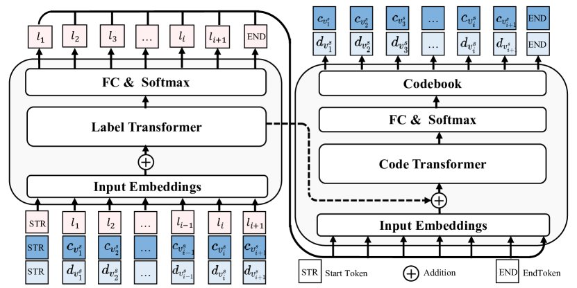
Figure 3: Network architecture of our generator.

Concretely, the label Transformer $\mathcal{T}^{l}$ takes as input the triplet $\left(\bm{c}_{v^{s}_{i}},\bm{d}_{v^{l}_{i}},l_{i}\right)$. Each element goes through its own embedding layer to get a feature, i.e., $\texttt{Emb}(\bm{c}_{v^{s}_{i}})\in\mathbb{R}^{512}$, $\texttt{Emb}(\bm{d}_{v^{l}_{i}})\in\mathbb{R}^{512}$, and $\texttt{Emb}(l_{i})\in\mathbb{R}^{512}$. The three features are simply added along the feature dimension to obtain the input feature for the attention blocks, which outputs a fused feature $\mathcal{F}_{\text{fuse}}$ after the attention calculation. $\mathcal{F}_{\text{fuse}}$ is then fed into a fully connected layer with the softmax activation to predict the one-hot probabilistic vector, which is translated into a one-hot class label $l_{i+1}\in\mathbb{R}^{C}$.

The code Transformer $\mathcal{T}^{c}$ accepts two inputs. The first one is $l_{i+1}$, which goes through an embedding layer to produce a conditional feature in $\mathbb{R}^{512}$. The second input is $\mathcal{F}_{\text{fuse}}$, which is also added with the conditional feature along the feature dimension to get the input feature for the attention block. Intuitively, the first input provides the direct semantic guidance of the current stroke, while the second input provides the shape and positional information of previous strokes. The attention blocks are followed by two separate branches, each of which outputs a one-hot probabilistic vector of dimension $\mathbb{R}^{V}$, indicating the indices of the shape and position codebooks. The corresponding code entries are fetched (i.e., $\bm{c}_{v^{s}_{i+1}}$ and $\bm{d}_{v^{l}_{i+1}}$) and serve as the input to the label Transformer for the next stroke generation.

Losses. To train the network, we minimize the negative log-likelihood loss, defined as:

$$\mathcal{L}_{\text{gen}}=-\log p(\bm{S}),$$ (5)

where we supervise the training with ground truth categorical labels (i.e., the shape label vector, shape code index vector, and the position code index vector).

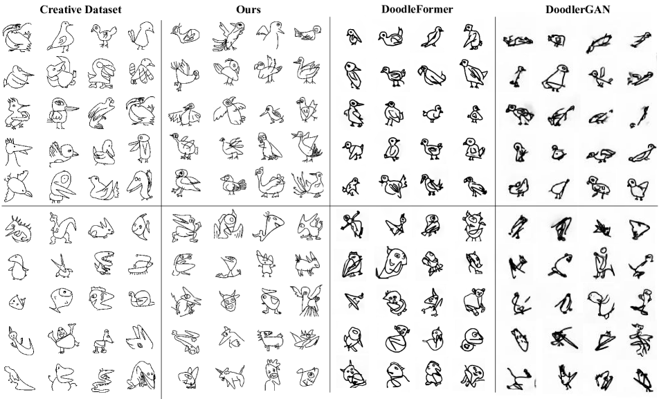
Figure 4: Visual comparison against competitors on both the Creative Birds and Creative Creatures datasets.

Training and testing strategy. We have three training stages. In the first stage, we train the stroke latent embedding auto-encoder. Once it is trained, both the encoder and decoder are fixed. In the second stage, we train the vector quantization auto-encoders and the corresponding codebooks. Similarly, once the network is trained, the three components are fixed. In the last stage, we train the cascaded generation decoders together, with the help of the aforementioned networks and codebooks. Note that, we follow [14] to address the teacher-forcing gap. For the testing time generation, starting from a special STR token, we generate novel strokes in an autoregressive manner, where the codebook entry is either decoded as the position quaternion or decoded as the stroke latent code, which is further converted into the corresponding rasterized image. The stroke triplet is finally assembled together to produce the resulting sketch (see Fig. 2, left).

4 Experiments

Implementation details. We use Adam optimizer[8] for training both the VQ-Representation and Gen-Transformer, while the learning rates are set as $10^{-4}$ for the former and $10^{-5}$ for the latter. We train our network on 2 NVIDIA V100 GPUs, which takes a total of 20 hours for the first and second training stages with a batch size of $64$, and around 10 hours for the generator with a batch size of $8$. The maximum stroke length $N$ is 20 for Creative Birds and 35 for Creative Birds to make sure it fits all the sketches. Stroke latent embedding $\bm{e}_{i}^{s}$ is a vector in $\mathbb{R}^{256}$. The number of codes $V$ = 8192, and the code dimensions of both codebooks are $512$. Stroke category number $C=8$ for Creative Birds and 17 for Creative Creatures. The balancing weight $\alpha=0.8$. Please refer to the supplementary for more details.

Datasets. Following previous work [5, 2], we use the CreativeSketch [5] dataset in this paper. Specifically, it consists of two categories of sketches — Creative Birds (CB) and Creative Creatures (CC) — containing 8,067 and 9,097 sketches, respectively, along with part annotations. All the sketches have been processed into 256 × 256 images. For the stroke latent embedding learning, we use strokes from both datasets to obtain a powerful pair of $\mathcal{E}^{s}$ and $\mathcal{D}^{s}$. Other than this autoencoder, we have trained other networks separately on CB and CC datasets. We have applied common stroke pre-processing steps, e.g., removing background strokes, discarding super-long strokes, and merging short strokes. See supplementary for more details about pre-processing and data augmentation.

Evaluation Metrics. Following previous work [5, 2], we evaluate the model’s performance using an Inception model  [17] trained on the QuickDraw3.8M dataset [26]. We use four metrics in this paper, defined as follows:

• Fréchet Inception Distance (FID) [6] measures the similarity between two image sets in the above Inception feature space.

• Generation diversity (GD) [3] measures the average pairwise Euclidean distance between the Inception features of two subsets, reflecting the diversity of the data item in the image set.

• Characteristic score (CS) measures how frequently a generated sketch is classified as Creative Bird or Creative Creature by the Inception model.

• Semantic diversity score (SDS) quantifies the diversity of sketches based on the various creature categories they represent.

Table 1: Statistical comparison against existing methods on Creative Birds and Creative Creatures datasets.

Methods	Creative Birds			Creative Creatures
	FID(↓)	GD(↑)	CS(↑)	FID(↓)	GD(↑)	CS(↑)	SDS(↑)
Training Data	-	19.40	0.45	-	18.06	0.60	1.91
Sketchknitter [24]	74.42	14.23	0.14	64.34	12.34	0.42	1.32
DoodlerGAN [5]	39.95	16.33	0.69	43.94	14.57	0.55	1.45
DoodleFormer [2]	17.48	17.83	0.57	20.43	16.23	0.53	1.68
Ours	15.78	18.92	0.53	17.61	17.42	0.57	1.86

4.1 Comparison

We compare our approach with three competitors, i.e., Doodleformer [2], DoodlerGAN [5], Sketchknitter [24], using the four metrics. Both Doodleformer and DoodlerGAN generate sketches at the pixel level, while Sketchknitter generates sketches at the stroke point sequence level. All three methods are trained using their default parameters on our dataset.

The quantitative comparison is presented in Tab. 1, where our method significantly outperforms others. Specifically, on the Creative Birds dataset, we obtained a notable 1.7 decrease in FID and gained a remarkable 1.09 increase in terms of GD, achieving the best performance. This indicates that our model can generate sketches that are closer to the original dataset, as well as more diverse at the same time. For the CS metric, while our approach does not achieve the highest score, it surpasses the dataset and comes closest to matching the dataset’s CS metric. In contrast, DoodlerGAN and DoodleFormer attain higher scores, whereas SketchKnitter’s outputs are seldom recognized as birds. For this specific metric, the higher value only means it is easier to be recognized by the Inception model, which may stem from the simplicity of the generation. The dataset’s value sets a good reference. Similarly, on the Creative Creatures dataset, we achieved the best performance across all four metrics. Specifically, we achieved a 2.82 decrease in FID and a 1.19 improvement in GD compared to the best other methods. This indicates that our generated sketches are closer to the more complex sketches in the training data and exhibit greater diversity among themselves. For the CS and SDS metrics, we obtained improvements of 0.04 and 0.18, respectively. This indicates that our generated sketches are semantically closer to the categories in the training data and also suggests that our model exhibits better semantic diversity. A corresponding visual comparison is shown in Fig. 4, where the artifacts like the broken and misaligned strokes from DoodlerGAN, and the blurry local regions from DoodleFormer, are clearly presented. In contrast, our results are of high quality with complex appearance and diverse shapes. Note that, as shown in Fig. 1, SketchKnitter generates poor results on both datasets, we did not include its results in the visual comparison.

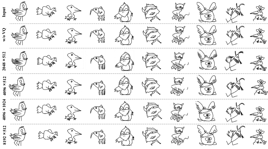
Figure 5: Sketch reconstruction results of our ablation study on codebook hyper-parameter setting. The two numbers represent the code size and the feature dimension, respectively.

Table 2: The statistical comparison of our ablation study. The method name of two numbers represents the codebook hyper-parameter setting, where the first is the code size, and the second is the feature dimension.

Methods	Creative Birds			Creative Creatures
	FID(↓)	GD(↑)	CS(↑)	FID(↓)	GD(↑)	CS(↑)	SDS(↑)
Training Data	-	19.40	0.45	-	18.06	0.60	1.91
2048$\times$512	26.23	15.34	0.43	43.21	14.51	0.48	1.52
4096$\times$512	16.92	18.27	0.50	18.44	16.14	0.54	1.63
4096$\times$1024	16.67	18.15	0.51	18.12	16.43	0.55	1.69
w/o $\mathcal{T}^{l}$	16.51	18.35	0.51	19.21	16.14	0.55	1.74
w/o VQ	48.53	13.34	0.46	54.56	14.02	0.45	1.36
w/o Decouple	17.14	18.12	0.57	19.42	16.42	0.56	1.79
Ours($8192\times 512$)	15.78	18.92	0.53	17.61	17.42	0.57	1.86

4.2 Ablation Study

To validate the effectiveness of our core technical components, we conducted experiments by removing them. Specifically, we form the following alternative solutions:

• w/o VQ: we remove all the codebook learning-related procedures, and use the continuous stroke latent embeddings to train our generator.

• w/o Decouple: we do not decouple the shape and position of the stroke, and only train a single stroke codebook. The Transformer decoders take fewer inputs and the second decoder outputs only one index vector accordingly.

• w/o $\mathcal{T}^{l}$: we simply discard the label information for each stroke, and remove the label Transformer accordingly.

We train the three alternatives from scratch using our datasets until convergence and statistical results are shown in Tab. 2. Without the VQ representation, the generator samples new sketches from a larger continuous space, instead of a compressed discretized space, giving the worst performance in this paper. The stroke decoupling matters the generation significantly (e.g., 15.78 $vs.$ 17.14 and 17.61 $vs.$ 19.42 of the FID). By decoupling, the shape code can concentrate only on the shape variation, while the position code can better capture the inherent approximation information between strokes, which further facilitates the generation. By removing the label prediction, we see a slight performance degradation, giving the second-best performance in Tab. 2. The labels are not very critical, but indeed provide semantic-related information to complement the positional information (e.g., the heads appear at similar positions with similar sizes).

Codebook hyper-parameter setting. There are two core hyper-parameters for a codebook, i.e., the code size and the feature dimension of the feature entry. We have conducted experiments to find the proper configuration. Specifically, we set the code size to be either 2,048, 4,096, or 8,192, and set the feature dimension to be either 512 or 1,024. We examine the effects of the parameter setting from both the sketch reconstruction and generation perspectives.

Figure 5 presents a visual comparison of the sketch reconstruction quality. By increasing either the code size or the feature dimension, we observe improved fidelity with less blurry and broken strokes. Note that the row named w/o VQ shows the stroke latent space reconstruction performance as in [23], which along with the input, provides a good performance reference. We chose the last configuration in this paper, as it gives the best visual reconstruction. However, it still struggles to represent strokes with significant variation, such as the ear of the creature in the third-to-last column. We further investigate the generation performance of different codebook settings. Quantitative results are listed in Tab. 2, where we observe improvement when increasing either the size of the code or the feature dimension. Our choice obtains the best result given the limited combination.

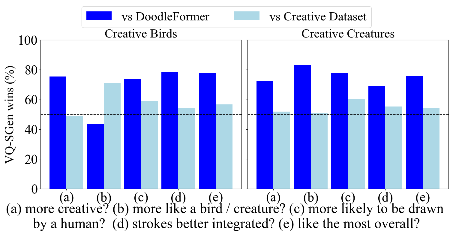
Figure 6: User study results based on the five questions (a-e). Higher scores indicate a stronger preference for our method over the other approaches (i.e., DoodleFormer or Creative datasets).

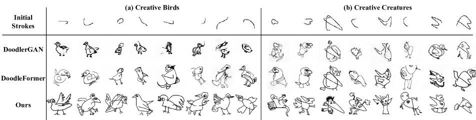
Figure 7: Visual comparison with competitors on conditional generation task.

4.3 User Study

Following [2, 5], we evaluate the performance of our method through user studies. We invited 50 participants to the test, where they were shown multiple pairs of images. Each pair consists of a sketch generated by our model and another sketch from either DoodleFormer or the datasets. For each pair, participants were asked to answer 5 single-choice questions: which one (a) is more creative? (b) looks more like a bird/creature? (c) is more likely to be drawn by a human? (d) the strokes better integrated? (e) they like the most overall? Figure 6 shows the percentage of times our method is preferred over the competing approach. It can be seen that VQ-SGen performs favorably against DoodleFormer for all five questions on both datasets except for question (b) on the Creative Birds dataset, which is consistent with the CS metric in Tab. 1. We are nearly tied with the creative datasets.

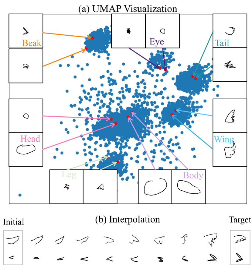
Figure 8: Code space exploration. (a) UMAP visualization of the shape codes in $\mathcal{D}^{s}$, with the overlaid strokes indicating the semantic aware clustering in the discrete code space. (b) Two code interpolation examples, where the interpolation is executed from the initial to the target strokes (left to right).

5 Discussion

Conditional Generation. Given an initial stroke, our model can perform conditional generation based on it. We achieve this by feeding the initial stroke as our first stroke in the generation process. Figure 7 presents a visual comparison against SoTA methods on this task. As can be seen, DoodlerGAN produced the worst results, with most sketches lacking a clear structure. DoodleFormer performed slightly better, but the generated sketches are often blurry and include ghost strokes (e.g., a few tail-like strokes of the first example in Fig. 7(b)). With the help of our VQ representation and our generator, our results are both creative and structurally coherent.

Code space exploration. To better understand the properties of the discrete space, we applied the UMAP algorithm [13] to project the high dimensional features of the shape codebook $\bm{D}^{s}$ into 2D space and visualize its distribution in Fig. 8(a). We further probe the emerged clustering by visualizing typical strokes. Not too surprised, we find that the emerged clusters correspond well to semantics. For example, the five surrounding clusters are Beak, Eye, Tail, Wing, and Leg, while the inner big cluster composed of Head and Body. Although we did not exploit any semantic-related constraints during the codebook learning, it tends to implicitly group strokes with similar shape variations, thereby achieving stable and efficient code learning and space compression. As a result, this provides an ideal foundation for the generator to sample new strokes within a semantically-aware, compressed space.

To further validate the clustering effects, we conduct code interpolation experiments. Fig. 8(b) demonstrates two such examples. The interpolation is executed from the initial stroke to the target stroke (left to right). We first use linear $\alpha$-blending to mix the two codes, and then fetch the closest code entry in $\mathcal{D}^{s}$ and decode it into a stroke image. We march 10 steps to achieve the target. As can be seen, the initial and target strokes can be meaningfully interpolated in the discrete code space.

Limitation. Firstly, the hyper-parameters of the codebooks might not be globally optimal. Efficient hyperparameter searching could potentially help. Secondly, we occasionally observe that the generated bounding box might not cover the outmost stroke, causing a hard cropping artifact. An extra coverage regularizer might help. We leave the two as future work.

6 Conclusion

In this paper, we have presented a novel approach to creative sketch generation. Our method can effectively create sketches with appealing appearance and coherent structures. We believe that stroke VQ representations can be used in other sketch-related tasks, and hope to inspire future research in sparse stroke representation learning.

Supplementary Material

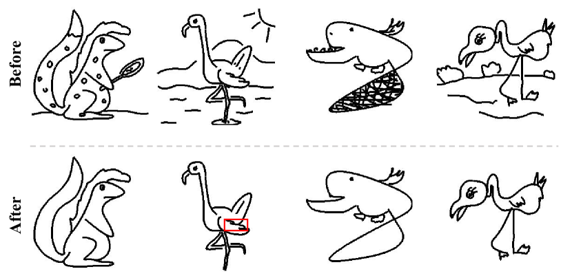
Figure 9: The demonstration of our data preprocessing.

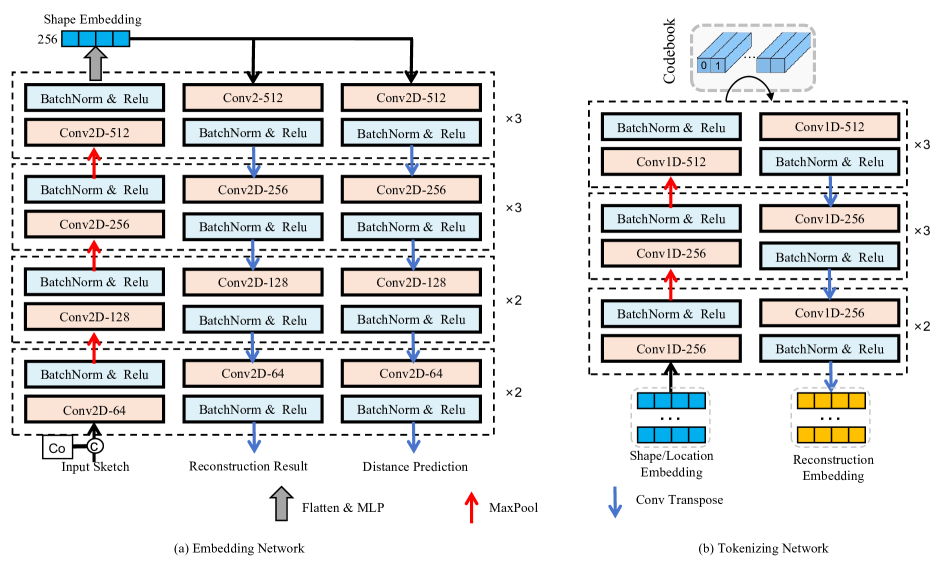
Figure 10: Detailed structure of our embedding networks and tokenizing network.

1 Data Preprocessing and Augmentation

To enhance the model’s performance and improve the quality of the training data, we adopt a series of preprocessing steps as shown in Fig. 9. Firstly, strokes that have the ’details’ part label (e.g., the sun, the ground, and the decorative dots) are moved, as these may introduce noise or unnecessary complexity. Secondly, excessively long strokes are eliminated to maintain a balanced distribution of stroke lengths (e.g., the over-sketched pattern in the tail of the third creature), preventing outliers from disproportionately influencing the model. Lastly, shorter strokes that are connected are merged into a single stroke to maintain a better stroke structure. For instance, the wing in the second image (highlighted with a red box) is composed of multiple connected strokes that are merged into a single stroke, which ensures more coherent and natural groupings within the sketches.

Besides preprocessing, we employ a comprehensive augmentation strategy at both the stroke and sketch levels. At the stroke level, transformations such as rotation, translation, or scaling are applied to one or more randomly selected strokes. These operations diversify the stroke representations and improve the model’s ability to generalize to various configurations. At the sketch level, the entire sketch is subjected to global transformations, including rotations or random removal of specific strokes, simulating incomplete or imperfect inputs.

2 Detailed Network Configuration

Intuitively, the stroke shape embedding and the learning of the codebook could be achieved simultaneously. However, the network responsible for learning stroke shape embeddings needs to be applied individually to each stroke to effectively capture its structural details, whereas the learning of the codebook must consider the entire sequence of strokes, performing the compression in the sketch level. Consequently, achieving optimal performance is challenging when attempting to combine these tasks. Therefore, we propose to handle them separately. To this end, we first convert each stroke into a latent embedding and further compress them in the latent space.

Figure 10 illustrates the detailed structure of our network. The embedding network has an encoder-decoder structure, accepting the grayscale stroke image input augmented with x and y coordinate channels. Specifically, the encoder comprises a total of 10 layers, which are grouped into four blocks. Each block is characterized by distinct feature dimensions (i.e., 64, 128, 256, and 512, respectively), resulting in a stroke embedding in $\mathbb{R}^{256}$. Both decoder branches share the encoder structure, working symmetrically to transform the stroke embedding into stroke reconstruction and the distance map as in [23].

We also illustrate the detailed network architecture of our tokenizing network, which is used for learning the shape or location codebook. The input is a feature matrix in $\mathbb{R}^{N\times 256}$ composed of shape or location embeddings within a sketch. A Conv1d layer is first employed for feature extraction, followed by a MaxPool layer or ConvTranspose1d layer to compress or expand the feature dimensions. Specifically, the encoder comprises 8 layers grouped into three blocks, each characterized by distinct feature dimensions (i.e., 256, 256, and 512), resulting in a feature of $\mathbb{R}^{N\times 512}$. The “x3” and “x2” of each block in Fig. 10 mean that the block is repeated 3 or 2 times. Subsequently, the feature corresponding to each stroke is replaced with the nearest code and then fed into the decoder. Both decoder branches share the encoder structure. The final output aims to reconstruct the latent input.

3 Training and Inference Details

We first train the VQ-Representation network until convergence, which takes around 20 hours with a batch size of 64. Then, the Gen-Transformer is trained until convergence taking around 10 hours with a batch size of 8. We set the learning rate as $10^{-4}$ for VQ-Representation network and $10^{-4}$ for Gen-Transformer. We use step decay for VQ-Representation with a step size equal to 10 and do not apply learning rate scheduling for Gen-Transformer.

Teacher Forcing Gap. Teacher-forcing strategy is widely used for Transformer training. However, it introduces the exposure bias issue by always feeding the ground truth information to the network at training time but exploiting the inferior prediction at testing time. To overcome this issue, we follow [14] to mix the predicted stroke information with the ground truth information. The ratio of the ground truth strokes gradually decreases from 1.0 as the training progresses.

Sampling in Inference. Starting with a special STR token, the inference process of our VQ-SGen generates a sketch by sequentially sampling each subsequent element of the stroke sequence until reaching an END token. Each prediction step consists of two stages: (1) generating a minimal set of codes for sampling, comprising the top options whose cumulative probabilities exceed a threshold $p_{n}$, while ignoring other low-probability codes; (2) performing random sampling within this minimal set based on the relative probabilities of the codes. This approach ensures diversity in the predicted code sequence while reducing the risk of sampling unsuitable or irrelevant codes.

4 Discussion of Limitation

Our network has the following limitations: First, we did not extensively explore all combinations of codebook hyperparameters, so our current configuration may not be globally optimal. This could impact the quality of our model’s generated results. For example, in Fig. 11(a), the wings exhibit stroke disconnection and blurring issues. Efficient hyperparameter search could potentially lead to improvements. Second, due to the decoupling of shape and position, we occasionally observe that the generated bounding box may fail to cover all strokes, resulting in a “hard cropping” of the outermost stroke. The strokes in the wings and head in Fig. 11(b) have experienced varying degrees of “hard cropping”. Introducing a coverage regularizer could help address this issue. We leave these two aspects as future work.

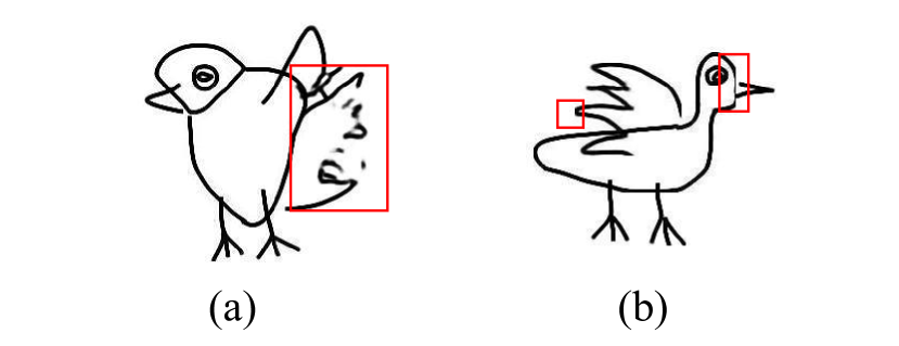
Figure 11: The demonstration of failure cases.

References

- Bandyopadhyay et al. [2024] Hmrishav Bandyopadhyay, Ayan Kumar Bhunia, Pinaki Nath Chowdhury, Aneeshan Sain, Tao Xiang, Timothy Hospedales, and Yi-Zhe Song. Sketchinr: A first look into sketches as implicit neural representations. In Proceedings of the IEEE/CVF Conference on Computer Vision and Pattern Recognition, pages 12565–12574, 2024.
- Bhunia et al. [2022] Ankan Kumar Bhunia, Salman Khan, Hisham Cholakkal, Rao Muhammad Anwer, Fahad Shahbaz Khan, Jorma Laaksonen, and Michael Felsberg. Doodleformer: Creative sketch drawing with transformers. In European Conference on Computer Vision, pages 338–355. Springer, 2022.
- Cao et al. [2019] Nan Cao, Xin Yan, Yang Shi, and Chaoran Chen. Ai-sketcher: a deep generative model for producing high-quality sketches. In Proceedings of the AAAI conference on artificial intelligence, pages 2564–2571, 2019.
- Chen et al. [2016] Xi Chen, Yan Duan, Rein Houthooft, John Schulman, Ilya Sutskever, and Pieter Abbeel. Infogan: Interpretable representation learning by information maximizing generative adversarial nets. Advances in neural information processing systems, 29, 2016.
- Ge et al. [2020] Songwei Ge, Vedanuj Goswami, C Lawrence Zitnick, and Devi Parikh. Creative sketch generation. arXiv preprint arXiv:2011.10039, 2020.
- Heusel et al. [2017] Martin Heusel, Hubert Ramsauer, Thomas Unterthiner, Bernhard Nessler, and Sepp Hochreiter. Gans trained by a two time-scale update rule converge to a local nash equilibrium. Advances in neural information processing systems, 30, 2017.
- Hinton and Salakhutdinov [2006] Geoffrey E Hinton and Ruslan R Salakhutdinov. Reducing the dimensionality of data with neural networks. science, 313(5786):504–507, 2006.
- Kingma and Ba [2014] Diederik P Kingma and Jimmy Ba. Adam: A method for stochastic optimization. arXiv preprint arXiv:1412.6980, 2014.
- Koley et al. [2024] Subhadeep Koley, Ayan Kumar Bhunia, Aneeshan Sain, Pinaki Nath Chowdhury, Tao Xiang, and Yi-Zhe Song. How to handle sketch-abstraction in sketch-based image retrieval? In Proceedings of the IEEE/CVF Conference on Computer Vision and Pattern Recognition, pages 16859–16869, 2024.
- Li et al. [2019] Ke Li, Kaiyue Pang, Yi-Zhe Song, Tao Xiang, Timothy M Hospedales, and Honggang Zhang. Toward deep universal sketch perceptual grouper. IEEE Transactions on Image Processing, 28(7):3219–3231, 2019.
- Li et al. [2018] Lei Li, Hongbo Fu, and Chiew-Lan Tai. Fast sketch segmentation and labeling with deep learning. IEEE computer graphics and applications, 39(2):38–51, 2018.
- Liu et al. [2018] Rosanne Liu, Joel Lehman, Piero Molino, Felipe Petroski Such, Eric Frank, Alex Sergeev, and Jason Yosinski. An intriguing failing of convolutional neural networks and the coordconv solution. Advances in neural information processing systems, 31, 2018.
- McInnes et al. [2018] Leland McInnes, John Healy, and James Melville. Umap: Uniform manifold approximation and projection for dimension reduction. arXiv preprint arXiv:1802.03426, 2018.
- Mihaylova and Martins [2019] Tsvetomila Mihaylova and André FT Martins. Scheduled sampling for transformers. arXiv preprint arXiv:1906.07651, 2019.
- Qi and Tan [2019] Yonggang Qi and Zheng-Hua Tan. Sketchsegnet+: An end-to-end learning of rnn for multi-class sketch semantic segmentation. Ieee Access, 7:102717–102726, 2019.
- Sain et al. [2021] Aneeshan Sain, Ayan Kumar Bhunia, Yongxin Yang, Tao Xiang, and Yi-Zhe Song. Stylemeup: Towards style-agnostic sketch-based image retrieval. In Proceedings of the IEEE/CVF conference on computer vision and pattern recognition, pages 8504–8513, 2021.
- Szegedy et al. [2016] Christian Szegedy, Vincent Vanhoucke, Sergey Ioffe, Jon Shlens, and Zbigniew Wojna. Rethinking the inception architecture for computer vision. In Proceedings of the IEEE conference on computer vision and pattern recognition, pages 2818–2826, 2016.
- Tang et al. [2024] Zecheng Tang, Chenfei Wu, Zekai Zhang, Mingheng Ni, Shengming Yin, Yu Liu, Zhengyuan Yang, Lijuan Wang, Zicheng Liu, Juntao Li, et al. Strokenuwa: Tokenizing strokes for vector graphic synthesis. arXiv preprint arXiv:2401.17093, 2024.
- Van Den Oord et al. [2017] Aaron Van Den Oord, Oriol Vinyals, et al. Neural discrete representation learning. Advances in neural information processing systems, 30, 2017.
- Vaswani [2017] A Vaswani. Attention is all you need. Advances in Neural Information Processing Systems, 2017.
- Vincent et al. [2010] Pascal Vincent, Hugo Larochelle, Isabelle Lajoie, Yoshua Bengio, Pierre-Antoine Manzagol, and Léon Bottou. Stacked denoising autoencoders: Learning useful representations in a deep network with a local denoising criterion. Journal of machine learning research, 11(12), 2010.
- Wang et al. [2020] Fei Wang, Shujin Lin, Hanhui Li, Hefeng Wu, Tie Cai, Xiaonan Luo, and Ruomei Wang. Multi-column point-cnn for sketch segmentation. Neurocomputing, 392:50–59, 2020.
- Wang and Li [2024] Jiawei Wang and Changjian Li. Contextseg: Sketch semantic segmentation by querying the context with attention. In Proceedings of the IEEE/CVF Conference on Computer Vision and Pattern Recognition, pages 3679–3688, 2024.
- Wang et al. [2023] Qiang Wang, Haoge Deng, Yonggang Qi, Da Li, and Yi-Zhe Song. Sketchknitter: Vectorized sketch generation with diffusion models. In The Eleventh International Conference on Learning Representations, 2023.
- Wu et al. [2018] Xingyuan Wu, Yonggang Qi, Jun Liu, and Jie Yang. Sketchsegnet: A rnn model for labeling sketch strokes. In 2018 IEEE 28th International Workshop on Machine Learning for Signal Processing (MLSP), pages 1–6. IEEE, 2018.
- Xu et al. [2022] Peng Xu, Timothy M Hospedales, Qiyue Yin, Yi-Zhe Song, Tao Xiang, and Liang Wang. Deep learning for free-hand sketch: A survey. IEEE transactions on pattern analysis and machine intelligence, 45(1):285–312, 2022.
- Yan et al. [2022] Xingguang Yan, Liqiang Lin, Niloy J Mitra, Dani Lischinski, Daniel Cohen-Or, and Hui Huang. Shapeformer: Transformer-based shape completion via sparse representation. In Proceedings of the IEEE/CVF Conference on Computer Vision and Pattern Recognition, pages 6239–6249, 2022.
- Yang et al. [2021] Lumin Yang, Jiajie Zhuang, Hongbo Fu, Xiangzhi Wei, Kun Zhou, and Youyi Zheng. Sketchgnn: Semantic sketch segmentation with graph neural networks. ACM Transactions on Graphics (TOG), 40(3):1–13, 2021.
- Zheng et al. [2018] Ningyuan Zheng, Yifan Jiang, and Dingjiang Huang. Strokenet: A neural painting environment. In International Conference on Learning Representations, 2018.
- Zheng et al. [2023] Yixiao Zheng, Jiyang Xie, Aneeshan Sain, Yi-Zhe Song, and Zhanyu Ma. Sketch-segformer: Transformer-based segmentation for figurative and creative sketches. IEEE Transactions on Image Processing, 2023.
- Zheng et al. [2024] Yixiao Zheng, Kaiyue Pang, Ayan Das, Dongliang Chang, Yi-Zhe Song, and Zhanyu Ma. Creativeseg: Semantic segmentation of creative sketches. IEEE Transactions on Image Processing, 33:2266–2278, 2024.
- Zhou et al. [2018] Tao Zhou, Chen Fang, Zhaowen Wang, Jimei Yang, Byungmoon Kim, Zhili Chen, Jonathan Brandt, and Demetri Terzopoulos. Learning to doodle with stroke demonstrations and deep q-networks. In BMVC, page 13, 2018.
- Zhu et al. [2018] Xianyi Zhu, Yi Xiao, and Yan Zheng. Part-level sketch segmentation and labeling using dual-cnn. In Neural Information Processing: 25th International Conference, ICONIP 2018, Siem Reap, Cambodia, December 13-16, 2018, Proceedings, Part I 25, pages 374–384. Springer, 2018.
- Zhu et al. [2020] Xianyi Zhu, Yi Xiao, and Yan Zheng. 2d freehand sketch labeling using cnn and crf. Multimedia Tools and Applications, 79(1-2):1585–1602, 2020.