Shortest Path Lengths in Poisson Line Cox Processes: Approximations and Applications

Abstract

We derive exact expressions for the shortest path length to a point of a Poisson line Cox process (PLCP) from the typical point of the PLCP and from the typical intersection of the underlying Poisson line process (PLP), restricted to a single turn. For the two turns case, we derive a bound on the shortest path length from the typical point and demonstrate conditions under which the bound is tight. We also highlight the line process and point process densities for which the shortest path from the typical intersection under the one turn restriction may be shorter than the shortest path from the typical point under the two turns restriction. Finally, we discuss two applications where our results can be employed for a statistical characterization of system performance: in a re-configurable intelligent surface (RIS) enabled vehicle-to-vehicle (V2V) communication system and in electric vehicle charging point deployment planning in urban streets.

I Introduction

Line or hyperplane processes are critical statistical models used to address various engineering issues in transportation and urban infrastructure planning, wireless communications, and industrial automation [1, 2]. In the Euclidean plane, these processes represent the set of points that constitute lines on the plane, where, the locations and orientations of the lines are specified on a parameter space according to a spatial point process. In particular, the Poisson line process (PLP) is a stochastic model used to describe random patterns of lines on a plane, where the lines are generated by a Poisson point process (PPP) in the parameter space. Researchers utilize line processes to investigate doubly stochastic processes called Cox processes, which are Poisson point processes constrained on the line process as their domain [3, 4, 5, 6, 7]. These models are instrumental in solving engineering questions, such as planning for the number of electric vehicle charging stations and bus stops, analyzing the cellular coverage performance for urban users with on-street deployments of wireless small cells [8], etc.

The $\ell_{1}$ distance is a metric that measures the shortest path between two points when the movement is restricted to the lines of the PLP. This is particularly important for transportation networks since it characterizes the distance traveled by a vehicle or pedestrian along the streets. Despite the relevance of this metric for practical applications, the characteristics and computational methods for $\ell_{1}$ distances in the Poisson line Cox process (PLCP) are not well understood. Fig. 1 illustrates the difference between the nearest neighbor with respect to the Euclidean distance in contrast to the same in terms of the path length. Although the nearest $\ell_{2}$ distance is simple to derive, e.g., see [9, 8], the same is not true for the shortest path-length or the $\ell_{1}$ distance.

Researchers have studied the shortest path length distributions for the case of the Manhattan line Cox process [10], where the orientations of the lines are restricted to a discrete set of two angles $\{0,\pi/2\}$. This was further extended to study dynamic charging of electric vehicles in [11]. For the PLCP model, the authors of [12] have proposed a method for simple computation of the mean shortest path lengths leveraging Neveu’s exchange formula [13]. The asymptotic behavior of this shortest path distance is investigated in [14]. However, due to the random orientation of the lines in a PLP, the exact characterization of the distribution of the shortest path length is challenging, and is still an open problem.

Contributions: Restricted to the one turn case (to be shortly defined), we provide an exact characterization of the shortest path length distribution to a point of the PLCP from the typical point of a PLCP and from the typical intersection of the underlying PLP. The case for the typical intersection is technically challenging and needs careful consideration of locations that are within a given path-length along both the lines constituting the typical intersection. Furthermore, we derive a bound on the shortest path length distribution for the two-turns case from the typical point of the PLCP. We study the conditions in which the path may be shorter for the one-turn case from the typical intersection as compared to the two-turn case starting from the typical point. Our results will find applications both in wireless network analysis, especially in vehicular communications, as well as planning of street systems. We discuss two such applications, one on optical vehicle-to-vehicle (V2V) communications that leverage re-configurable intelligent surface (RIS) and the other on planning for the placement of electric vehicle charging points.

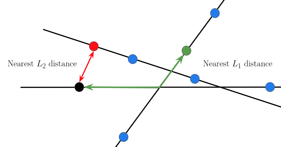
Figure 1: Illustration of the nearest $\ell_{2}$ vs $\ell_{1}$ distances. From the perspective of the typical point (black), the red point is the nearest point of the PLCP in the Euclidean plane, while, the green point is the nearest point from a path length perspective.

II Background and Notation

A line process in $\mathbb{R}^{2}$ is a set of points in $\mathbb{R}^{2}$ that constitute a set of lines. Each line $L_{i}$ is uniquely characterized by its signed distance $r_{i}$ from the origin and the angle $\theta_{i}$ that the normal to the line makes with the $x-$axis. The parameter pair $(\theta_{i},r_{i})$ thus resides as a point in a parameter space $[0,\pi)\times(-\infty,\infty)$ that generates the line $L_{i}$ in $\mathbb{R}^{2}$.

Definition 1.

A line process $\mathcal{P}\subset\mathbb{R}^{2}$ is called a PLP iff the generating points form a PPP on the parameter space $[0,\pi)\times(-\infty,\infty)$ with a constant density $\lambda$.

Then, the points of the PLP that comprise $L_{i}\subset\mathcal{P}$ is the set $\{(x,y)\in\mathbb{R}^{2}:x\cos\theta_{i}+y\sin\theta_{i}=r_{i}$ for some $(\theta_{i},r_{i})\in[0,\pi)\times(-\infty,\infty)\}$. Let us consider one such PLP $\mathcal{P}$ where the intensity of the generating points is $\lambda$. On each $L_{i}\subset\mathcal{P}$, let us define a one dimensional PPP $\Phi_{i}\subset L_{i}$ with intensity $\mu$. The collection of all such one dimensional PPPs on all such lines $\Phi\coloneq\cup_{i:L_{i}\subset\mathcal{P}}\Phi_{i}$ is called a PLCP with intensity parameters $\lambda$ and $\mu$. Furthermore, we denote by $I_{ij}$ as the point of intersection of $L_{i}$ and $L_{j}$, and define the intersection process as $\Phi_{\rm I}\coloneq\cup_{i,j:L_{i},L_{j}\subset\mathcal{P}}I_{ij}=\cup_{i,j\in\mathcal{P}}L_{i}\cap L_{j}$. We perform our analysis from the perspective of the typical point of $\Phi$. In particular, let us define

$$\Phi^{o}\triangleq(\Phi\mid o\in\Phi),$$

and note that under expectation over $\Phi^{o}$, $o$ becomes the typical point of the process $\Phi$. Since by construction, $\Phi$ is a stationary process, let us consider $o$ to be the origin of $\mathbb{R}^{2}$. Under Palm conditioning, there exists a line $L_{\rm x}$ passing through $o$. Without loss of generality, let us consider $L_{\rm x}$ to be the $x-$axis. Let the lines intersecting $L_{\rm x}$ be enumerated (in no particular order) by the elements of the set $\{L_{i}\}$, $i\in\mathbb{N}$ and the corresponding intersections be $\{I_{i}\}$. Let the distance of $I_{i}$ from the origin be denoted by $s_{i}$ and the angle between $L_{1}$ and $L_{\rm x}$ be denoted by $\theta_{i}$. Let $D$ denote the length of the shortest path from the typical point to the nearest neighbor of the PLCP. Mathematically,

$$D=\min_{x\in\Phi^{!o}}\|x\|_{1},$$

where $\Phi^{!o}$ is the reduced Palm process constructed by assuming the typical point to be a part of $\Phi$ and then by removing the typical point.

II-A Limitation of a trivial approximation

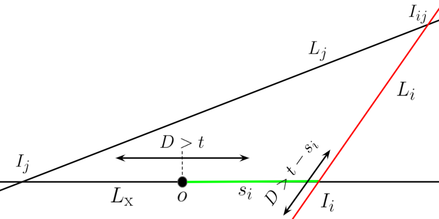
Figure 2: Approximation using recursive equations

Note that a simple approximation as illustrated in Fig. 2 follows by assuming that the distribution of the shortest path length from the typical PLCP point is the same as the distribution of the shortest path length from $I_{i}$ conditioned on the event that the path from $I_{i}$ cannot start along $L_{\rm x}$ but along $L_{i}$. In Fig. 2 it means that at $I_{i}$, we remove the line $L_{\rm x}$ and consider $I_{i}$ as the surrogate of the typical point and study the event $D>t-s_{i}$. Mathematically, this results in the following recursive equation.

$$\mathbb{P}(D>t)= \exp\left(-\mu t\right)\sum_{k}p_{k}(t)\left(\frac{1}{t}\int_{0}^{t}\mathbb{P}(D>t-s)\,ds\right)^{k},$$

where $p_{k}(t)\coloneq\exp\left({-2\lambda t}\right)\frac{(2\lambda t)^{k}}{k!},$ is the probability that there are $k$ intersections within a distance $t$ from the typical point. Conditioned on $k$, the distances of these intersections are independent and identically (in fact uniformly) distributed in $[0,t]$. As per the approximation, given that an intersection is at a distance $s$ from the typical point on $L_{\rm x}$, for no points within a path length $t$ from the typical point, we are interested in the event $D>t-s$ from the intersection. Thus, we get

$$\mathbb{P}(D>t)=\exp\left(-\mu+2\lambda\right)t\sum_{k}\frac{1}{k!}\left(2\lambda\int_{0}^{t}\mathbb{P}(D>t-s)\,d{\rm s}\right)^{k},$$

Now defining $u(t)\coloneq\mathbb{P}(D>t)$, $I(t)\coloneq\int_{0}^{t}u(t-s)\,d{\rm s}$ and differentiating with respect to $t$ we obtain the following differential equation.

$$u^{\prime}(t) =\exp\left(-(\mu+2\lambda)t\right)\sum_{k}\frac{1}{(k-1)!}\left(2\lambda\int_{0}^{t}u(t-s)\,{\rm d}s\right)^{k-1}$$

$$\frac{{\rm d}}{{\rm d}t}\left(2\lambda\int_{0}^{t}u(t-s)\,ds\right)-(\mu+2\lambda)u(t)$$

$$=\exp\left({-(\mu+2\lambda)t}\right)2\lambda\sum_{k}\frac{1}{(k-1)!}$$

$$\left(2\lambda t\int_{0}^{t}u(t-s)\,ds\right)^{k-1}-(\mu+2\lambda)u(t)$$

$$=2\lambda u(t)-(\mu+2\lambda)u(t)=-\mu u(t).$$

This solution results in

$$\mathbb{P}\left(D>t\right)=\exp(-\mu t),$$

which is incidentally the same as the probability of no PLCP point being located within a distance $t$ on $L_{\rm x}$ from the typical point. This occurs due to the fact that while approximating the path length from $I_{i}$ to be $D$, we over-count segments of the PLP, e.g., the segment between the typical point and $I_{i}$ shown in green in Fig. 2. This motivates the need for a more careful characterization of the path length distribution.

III Single Turn Case

Let us first consider the distribution of the distance to the nearest neighbor from the typical point under the restriction that only those PLCP points are considered that are reachable by traversing at most two lines $L_{i}$, including $L_{\rm x}$. Within this restriction, we consider two cases: first where the origin is the typical point and second where the origin is the typical intersection.

(a)

(b)

Figure 3: All the green colored points are within a distance $t$ by taking at most one turn from the origin (black point) when (a) the origin is the typical point of the PLCP and (b) the origin is the typical intersection of the PLP.

III-A From the typical point

Let the number of intersections from the origin within a distance $t$ be $N_{t}$. Furthermore, let $[N_{t}]$ denote the set $\{1,2,\ldots,N_{t}\}$. As per the property of PLP, $N_{t}$ is Poisson distributed with intensity $2\lambda t$ [4]. Accordingly, the complementary cumulative distribution function (CCDF) of $D$ is evaluated as one minus the void probability, which is calculated as follows.

Theorem 1.

Restricted to the single turn case, the distribution of the shortest path length from the typical point of the PLCP to another point of the PLCP is

$$F_{D}(t)=1-\exp\left(-2\mu t-2\lambda t+\frac{\lambda}{\mu}\left(1-\exp\left(-2\mu t\right)\right)\right).$$ (1)

Proof:

The shortest path length distribution follows directly from the void probability $\mathbb{P}(D>t)$. Let us consider the counting measure notation for the point processes [15], where $\Phi(A)$ denotes the number number of points of $\Phi$ within a path length $A$. Furthermore, $\Phi_{\rm x}$ represents the PPP on $L_{\rm x}$. Then, the CCDF is evaluated as:

$$\mathbb{P}\left(D>t\right)=\mathbb{P}\left(\Phi_{\rm x}(t)=0,\cup_{i:s_{i}\leq t}\Phi_{i}(t-s_{i})=0\right)$$

$$\overset{(a)}{=}\mathbb{P}\left(\Phi_{\rm x}(t)=0\right)\cdot\mathbb{P}\left(\cup_{i:s_{i}\leq t}\Phi_{i}(t-s_{i})=0\right)$$

$$\overset{(b)}{=}\exp(-2\mu t)\left[\sum_{k=0}^{\infty}\frac{\exp(-2\lambda t)(2\lambda t)^{k}}{k!}\right.$$

$$\hskip 56.9055pt\left.\left(\frac{1}{t}\int_{0}^{t}\exp(-2\mu(t-s)){\rm d}s\right)^{k}\right]$$

$$=\exp\left(-2\mu t-4\lambda t+\frac{2\lambda}{\mu}\left(1-\exp\left(-2\mu t\right)\right)\right).$$

The step (a) follows from the independence of the PPPs defined on the lines of the PLP. The step (b) follows from the Poisson distribution of the number of lines. Finally, one minus the void probability gives the relevant distance distribution. ∎

Remark 1.

Note that the expression for the void probability is composed of three different terms: $\exp\left(-2\mu t\right)$ that represents the probability that no PLCP points is present within $t$ in $L_{\rm x}$; the term $\exp\left(-4\lambda t\right)$ corresponds to the event that no line intersects within a distance $t$ from the typical point; while, considering the fact that for the void event, lines can intersect within $t$ as long as they do not contain any points within a distance $t-s_{i}$, the second term is weighted by the positive quantity $\exp\left(\frac{2\lambda}{\mu}(1-\exp(-2\mu t))\right)$.

III-B From the typical intersection

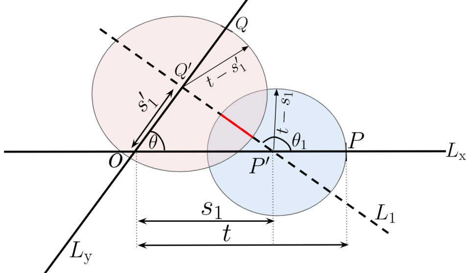
Figure 4: The single turn case starting from the typical intersection.

Next, let us consider the typical intersection $O$ depicted in Fig. 4. Here, unlike the previous case, under Palm conditioning, there exists two lines passing through the typical intersection, denoted by $L_{\rm x}$ and $L_{\rm y}$, respectively. To be precise, we define the conditioned line process $\mathcal{P}^{o}$ as

$$\mathcal{P}^{o}\triangleq(\mathcal{P}|L_{\rm x},L_{\rm y}\in\mathcal{P}),$$ (2)

where $L_{\rm x}$ and $L_{\rm y}$ are two lines with a uniformly distributed angle of intersection. Then, under expectation over $\mathcal{P}^{o}$, the intersecting point $O$ becomes the typical intersection. Let the angle between $L_{\rm x}$ and $L_{\rm y}$ be denoted by $\theta$. Similar to the case of the typical point, the nearest neighbor distribution $\mathbb{P}(D\leq t)$ here is obtained from the void probability depending on path length $t$. Let the random variable $Z_{1}$ denote the length of the lines of $\mathcal{P}$ wherein no point of $\Phi$ should be present for the event $D>t$ to hold. First, we characterize $Z_{1}$ for different cases of intersection locations of lines $L_{1}$ on $L_{\rm x}$ and $L_{\rm y}$. Then, we average out over all possible such $L_{1}$ within $t$ to obtain the final result.

Theorem 2.

The distribution of the distance to the nearest PLCP point from the typical intersection of the PLP is

$$F_{D}(t)=1-\exp\left(-4\mu t-2\lambda\left(2t-\mathcal{T}_{x}-\mathcal{T}_{y}\right)\right),$$ (3)

where

$$\mathcal{T}_{x}=\frac{1}{\pi^{2}}\int_{0}^{\pi}\int_{0}^{t}\int_{0}^{\pi}\exp\left(-\mu Z(x,\omega_{1},\omega)\right){\rm d}\omega_{1}{\rm d}x{\rm d}\omega,$$

$$\mathcal{T}_{y}=\frac{1}{\pi^{2}}\int_{0}^{\pi}\int_{0}^{t}\int_{\theta_{\mathcal{E}_{1,1}}}^{\theta_{\mathcal{E}_{1,2}}}\exp\left(-\mu Z(x,\omega_{1},\omega)\right){\rm d}\omega_{1}{\rm d}x{\rm d}\omega,$$

and

$$Z(x,\omega_{1},\omega)=$$

$$\begin{cases}2t-x\left(\frac{\sin\omega-\sin\omega_{1}}{\sin(\omega_{1}-\omega)}+1\right);\omega_{1}\in[0,\theta_{\mathcal{E}_{2,1}}]\cup[\theta_{\mathcal{E}_{2,2}},\pi]\\ 2(t-x);\quad\theta_{1}\in[\theta_{\mathcal{E}_{1,1}},\theta_{\mathcal{E}_{1,2}}]\\ 4t-2x\left(1+\frac{2\sin\omega_{1}}{\sin(\omega_{1}-\omega)}\right);\omega_{1}\in[\theta_{\mathcal{E}_{2,1}},\theta_{\mathcal{E}_{1,1}}]\cup[\theta_{\mathcal{E}_{1,2}},\theta_{\mathcal{E}_{2,2}}].\end{cases}$$

The ranges of $\theta_{1}$ in the above equation are as follows.

$$\theta_{\mathcal{E}_{1,1}}=\arctan\left(\frac{t\sin\omega}{t\cos\omega-x}\right),$$

$$\theta_{\mathcal{E}_{1,2}}=\arctan\left(\frac{t\sin\omega}{x+t\cos\omega}\right),$$

$$\theta_{\mathcal{E}_{2,1}}=\arccos\left(\frac{\left(\left(\frac{2t-x}{x}\right)^{2}+1\right)\cos\omega+2\left(\frac{2t-x}{x}\right)}{2\left(\frac{2t-x}{x}\right)\cos\omega+\left(\frac{2t-x}{x}\right)^{2}+1}\right),$$

$$\theta_{\mathcal{E}_{2,2}}=\arccos\left(\frac{\left(\left(\frac{2t-x}{x}\right)^{2}+1\right)\cos\omega-2\left(\frac{2t-x}{x}\right)}{-2\left(\frac{2t-x}{x}\right)\cos\omega+\left(\frac{2t-x}{x}\right)^{2}+1}\right).$$

Proof:

From the typical intersection, under the restriction of at most one turn, we can traverse either $L_{\rm x}$ or $L_{\rm y}$, but not both. Additionally, note that across realizations of $\mathcal{P}^{o}$, all the other lines almost surely intersect both $L_{\rm x}$ and $L_{\rm y}$. Let us consider one such line, $L_{1}$, that intersects $L_{\rm x}$ at $P^{\prime}$ at a distance $s_{1}$ from the origin and $L_{\rm y}$ at $Q^{\prime}$ at a distance $s^{\prime}_{1}$ from the origin. Naturally,

$$s^{\prime}_{1}=\frac{s_{1}\sin\theta_{1}}{\sin(\theta_{1}-\theta)}.$$ (4)

The length of the segment of intersection $|P^{\prime}Q^{\prime}|$ has two equivalent forms for given $s_{1}$, $\theta$, and $\theta_{1}$:

$$|P^{\prime}Q^{\prime}| =\frac{s_{1}\sin\theta}{\sin(\theta_{1}-\theta)}=\frac{s^{\prime}_{1}\cos\theta-s_{1}}{\cos\theta_{1}},$$ (5)

where $s^{\prime}_{1}$ is given by (4). Now conditioned on $\theta$ and $s_{1}$ consider the following events: (i) the event $\mathcal{E}^{c}_{1}$ (complement of event $\mathcal{E}_{1}$) defined as the case $s^{\prime}_{1}>t$. In this case, for the shortest path to be of length less than $t$ and the corresponding point to lie on $L_{1}$, the path can only be via the intersection $I_{{\rm x}1}$ and not via $I_{{\rm y}1}$; and (ii) the joint event $\mathcal{E}_{2}\mathcal{E}_{1}$ defined as $|P^{\prime}Q^{\prime}|\leq(t-s_{1})+(t-s^{\prime}_{1})$ and $s^{\prime}_{1}\leq t$. In this case, the both $I_{{\rm x}1}$ and $I_{{\rm y}1}$ are feasible intersection points distances less than $t$ on $P^{\prime}Q^{\prime}$. We convert the above conditions on $s^{\prime}_{1}$ to corresponding conditions on $\theta_{1}$, given $s_{1}$ and $\theta$. Note that $\theta_{1}=\arctan\left(\frac{s^{\prime}_{1}\sin\theta}{s^{\prime}_{1}\cos\theta-s_{1}}\right)$. Thus, for $s^{\prime}_{1}>t$, we have

$$\theta_{1}>\arctan\left(\frac{t\sin\theta}{t\cos\theta-t}\right)=\theta_{\mathcal{E}_{1,1}}.$$ (6)

Similarly, let $\theta_{\mathcal{E}_{1,2}}$ be the angle for which $L_{1}$ intersects $L_{\rm y}$ at a distance $t$ from the origin below the x-axis. For that case, we find a similar angle $\theta_{\mathcal{E}_{1,2}}=\arctan\left(\frac{t\sin\theta}{s_{1}+t\cos\theta}\right)$. Thus, the event $\mathcal{E}^{c}_{1}$ is equivalent to $\theta_{1}\in(\theta_{\mathcal{E}_{1,1}},\theta_{\mathcal{E}_{1,2}})$. Since for the event $\mathcal{E}^{c}_{1}$, any point within a distance $t$ on $L_{1}$ is reachable only from the $I_{{\rm x}1}$ intersection, for such a point to not exist, we calculate the void probability in a segment of length $Z_{1}(s_{1},\theta,\phi)=2(t-s_{1})$ on $L_{1}$.

Next let us study the event $\mathcal{E}_{1}\mathcal{E}_{2}$. Following the same steps as before, we note that if $L_{1}$ intersects $L_{\rm y}$ above the $x-$axis, then the event $\mathcal{E}_{2}$ corresponds to $\frac{s^{\prime}_{1}\sin\theta}{\sin(\theta_{1}-\theta)}<2t-s_{1}-\frac{s_{1}}{\sin(\theta_{1}-\theta)}$, or

$$\pi\geq\theta_{1} >\arccos\left(\frac{\left(\left(\frac{2t-s_{1}}{s_{1}}\right)^{2}+1\right)\cos\theta-2\left(\frac{2t-s_{1}}{s_{1}}\right)}{-2\left(\frac{2t-s_{1}}{s_{1}}\right)\cos\theta+\left(\frac{2t-s_{1}}{s_{1}}\right)^{2}+1}\right)$$

$$=\theta_{\mathcal{E}_{2,2}}.$$ (7)

On the contrary, in case $L_{1}$ intersects $L_{\rm y}$ below the $x-$axis, the event $\mathcal{E}_{2}$ corresponds to

$$0\leq\theta_{1} \leq\arccos\left(\frac{\left(\left(\frac{2t-s_{1}}{s_{1}}\right)^{2}+1\right)\cos\theta+2\left(\frac{2t-s_{1}}{s_{1}}\right)}{2\left(\frac{2t-s_{1}}{s_{1}}\right)\cos\theta+\left(\frac{2t-s_{1}}{s_{1}}\right)^{2}+1}\right)$$

$$=\theta_{\mathcal{E}_{2,1}}.$$ (8)

Thus, the joint event $\mathcal{E}_{1}\mathcal{E}_{2}$ corresponds to $\theta_{1}\in[0,\theta_{\mathcal{E}_{2,1}})\cup(\theta_{\mathcal{E}_{2,2}},\pi]$. For this case, the length of interest on $L_{1}$ where no points should reside is evaluated as

$$Z_{1}(s_{1},\theta,\theta_{1})=2t-s_{1}\left(\frac{\sin\theta+\sin\theta_{1}}{\sin(\theta_{1}-\theta)}+1\right).$$ (9)

Finally, for the event $\mathcal{E}_{1}\mathcal{E}^{\rm c}_{2}$, we have $\theta_{1}\in[\theta_{\mathcal{E}_{2,1}},\theta_{\mathcal{E}_{1,1}}]\cup[\theta_{\mathcal{E}_{1,2}},\theta_{\mathcal{E}_{2,2}}]$. In this case,

$$Z_{1}(s_{1},\theta,\theta_{1})=4t-2s_{1}\left(1+\frac{\sin\theta_{1}}{\sin(\theta_{1}-\theta)}\right).$$ (10)

Let $\mathcal{P}_{\rm x}\subset\mathcal{P}$ denote the set of lines that intersect $L_{\rm x}$ within a distance $t$ from the origin. Furthermore, let $\mathcal{P}^{\prime}_{\rm y}\subset\mathcal{P}$ denote the set of lines that intersect $L_{\rm y}$ within a distance $t$ from the origin and intersect $L_{\rm x}$ outside a distance $t$ from the origin. Based on the above characterization, we proceed with our derivation of the void probability as follows.

$$\mathbb{P}\left(D>t\right)=\mathbb{P}\left(\Phi_{\rm x}(t)=0,\Phi_{\rm y}(t)=0,\cup_{\mathcal{P}_{\rm x}}\Phi_{i}(t-s_{i})\right.$$

$$\hskip 56.9055pt\left.\cup_{\mathcal{P}^{\prime}_{\rm y}}\Phi_{j}(t-s^{\prime}_{i})=0\right)$$

$$=\mathbb{P}\left(\Phi_{\rm x}(t)=0\right)\mathbb{P}\left(\Phi_{\rm y}(t)=0\right)\mathbb{P}\left(\Phi\cap\left(\cup_{i\in\mathcal{P}_{\rm x}}Z_{i}\right)=0\right)$$

$$\hskip 56.9055pt\mathbb{P}\left(\Phi\cap\left(\cup_{i\in\mathcal{P}^{\prime}_{\rm y}}Z_{i}\right)=0\right)$$

$$=\exp\left(-4\mu t\right)\cdot$$

$$\left[\sum_{k=0}^{\infty}\frac{p_{k}(t)}{\pi^{2}t}\left(\int_{0}^{\pi}\int_{0}^{t}\int_{0}^{\pi}\exp\left(-\mu Z(x,\omega_{1},\omega)\right)d\omega_{1}{\rm d}x{\rm d}\omega\right)^{k}\right]$$

$$\left[\sum_{k=0}^{\infty}\frac{p_{k}(t)}{\pi^{2}t}\left(\int_{0}^{\pi}\int_{0}^{t}\int_{\phi_{\mathcal{E}_{1,1}}}^{\phi_{\mathcal{E}_{1,2}}}\exp\left(-\mu Z(x,\omega_{1},\omega)\right)\right.\right.$$

$$\left.\left.{\rm d}\omega_{1}{\rm d}xd\omega\right)^{k}\right]$$

$$=\exp\left(-4\mu t-2\lambda\left(2t-\mathcal{T}_{x}-\mathcal{T}_{y}\right)\right).$$ (11)

∎

Remark 2.

In Theorem 2, the term $\exp(-4\mu t)$ corresponds to the probability that no point located in either $L_{\rm x}$ or $L_{\rm y}$ within a distance $t$. The term $\exp(-4\lambda t)$ is the probability that no lines should be present with a distance $t$ from the origin along $L_{\rm x}$ or $L_{\rm y}$. However, for the void event such lines can be present given that they do not contain any PLCP points within a path length $t$ from the origin. Consequently, the probability is augmented by the factor $\exp(2\lambda\mathcal{T}_{\rm x})\cdot\exp\left(2\lambda\mathcal{T}_{\rm y}\right)$. The first term takes into account the region along the lines of $\mathcal{P}_{\rm x}$ while the second term does so for the lines of $\mathcal{P}^{\prime}_{\rm y}$.

Corollary 1 (Zero Turn Case).

The cumulative density function (CDF) of $D$ is lower bound as

$$F_{D}(t)\geq 1-\exp\left(-4\mu t\right).$$ (12)

Proof:

This is derived by considering the void probability of $(\Phi_{\rm x}\cup\Phi_{\rm y})\cap\mathcal{B}(0,t)$, where $\Phi_{\rm x}$ and $\Phi_{\rm y}$ respectively represent the points of $\Phi$ on $L_{\rm x}$ and $L_{\rm y}$, and $\mathcal{B}(0,t)$ represents a ball of radius $t$ centered at the typical intersection. ∎

Corollary 2 (Upper bound).

The CDF of $D$ is upper bounds as

$$F_{D}(t)\leq 1-\exp\left(-4(\mu+4\lambda)t\right).$$ (13)

Proof:

The upper bound is derived by considering the void probability of $(\Phi_{\rm x}\cup\Phi_{\rm y}\cup\Phi_{\rm Ix}\cup\Phi_{\rm Iy})\cap\mathcal{B}(0,t)$, where $\cup\Phi_{\rm Ix}$ and $\cup\Phi_{\rm Iy}$ are the intersection in $\Phi_{\rm I}$ present along $L_{\rm x}$ and $L_{\rm y}$, respectively. ∎

The above completes an exact characterization of the distribution of the distance to the nearest PLCP point from either the typical point or from the typical intersection restricted to one turn. The next section extends these results to approximate the two-turns case.

IV Two Turns From The Typical Point

For the two turns case, we restrict our analysis to the case where starting from the origin, we are allowed to move only in a given direction (without loss of generality, let us consider this to be along the positive direction of the x-axis).

Theorem 3.

The distribution of the nearest PLCP point from the typical point of the PLCP under the restriction of two-turns along a single direction is bounded as

$$\mathbb{P}\left(D\leq t\right) \leq 1-\exp\left(-\lambda\int_{0}^{t}2-\exp\left(-\lambda\int_{0}^{u}2-\right.\right.$$

$$\left.\left.T(w,u)f_{s_{i}|s_{1}}(w){\rm d}w\right)f_{s_{1}}(u){\rm d}u\right),$$ (14)

where, $f_{s_{i}|s_{1}}(w)=\frac{1}{s_{1}}$ for $0\leq w\leq s_{1}$, $f_{s_{1}}(u)=\frac{1}{t}$ for $0\leq u\leq t$. The innermost integrand is

$$T(w,u)=\mathds{1}\left(\mathcal{E}_{i}\right)\iint_{\theta_{i},\theta_{1}\in\mathcal{E}_{i}}\exp\left(-\mu\left(t-\right.\right.$$

$$\left.\left.\left(\frac{u-w}{\cos\theta_{i}-\sin\theta_{i}\cot\theta_{1}}+w\right)\right)\right){\rm d}\theta_{1}{\rm d}\theta_{i}+\left(1-\mathds{1}\left(\mathcal{E}_{i}\right)\right)\infty.$$ (15)

The event $\mathcal{E}_{i}$ is defined with the following conditions on $\theta_{i}$ and $\theta_{1}$ as follows.

$$\mathcal{E}_{i}=\begin{cases}\theta_{1}\leq{\rm cot}^{-1}\left(\cos\theta_{i}-\left(\frac{u-w}{t-w}\right)\csc\theta_{i}\right);\quad 0\leq\theta_{i}\leq\frac{\pi}{2},\\ \theta_{1}>{\rm cot}^{-1}\left(\left(\frac{u-w}{t-w}-\cos\theta_{i}\right)\csc\theta_{i}\right);\quad\frac{\pi}{2}<\theta_{i}\leq\pi.\end{cases}$$

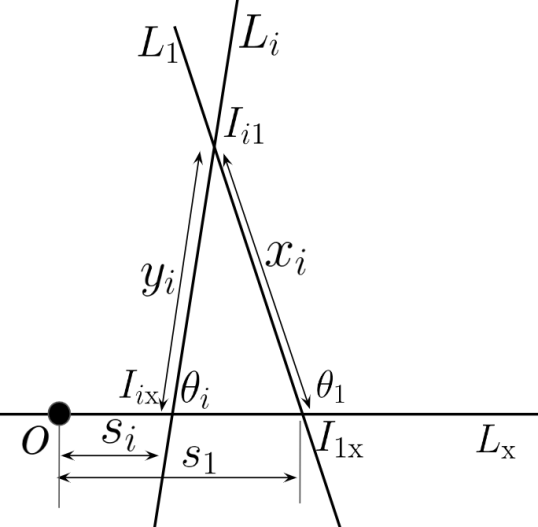
Figure 5: The two turns case. $L_{1},L_{2},\ldots$ intersect the line $L_{\rm x}$.

Proof:

Let us consider the intersection formed by two lines $L_{1}$ and $L_{i}$ that cross $L_{\rm x}$ at distances $s_{1}$ and $s_{i}$, respectively, from the origin such that $0\leq s_{i}\leq s_{1}\leq t$. Let us denote by $x_{i}$ the distance between the intersection $I_{i1}$ and $I_{1X}$. Similarly, $y_{i}$ denotes the distance between $I_{i1}$ and $I_{iX}$. Naturally, we have

$$x_{i}=\frac{y_{i}\sin\theta_{i}}{\sin\theta_{1}},\quad\text{ and }y_{i}=\frac{d_{i}}{\cos\theta_{i}-\sin\theta_{i}\cot\theta_{1}}.$$

From the intersection $I_{i1}$, along the line $L_{1}$, we have a remaining path-length budget of $z_{i}=\max\{0,t-(y_{i}+s_{i})\}$. Thus, we need conditions on $\theta_{1}$ and $\theta_{i}$ that correspond to the event $\mathcal{E}_{i}\coloneq\{y_{i}+s_{i}\leq t\}$. This evaluates to

$$\mathcal{E}_{i}\coloneq\begin{cases}\theta_{1}\leq{\rm cot}^{-1}\left(\cos\theta_{i}-\left(\frac{d_{i}}{t-s_{i}}\right)\csc\theta_{i}\right);\quad 0\leq\theta_{i}\leq\frac{\pi}{2},\\ \theta_{1}>{\rm cot}^{-1}\left(\left(\frac{d_{i}}{t-s_{i}}-\cos\theta_{i}\right)\csc\theta_{i}\right);\quad\frac{\pi}{2}<\theta_{i}\leq\pi.\end{cases}$$

Accordingly, $z_{i}$ takes a value 0 in the event $\mathcal{E}^{c}_{i}$ (the event that no path length budget remains once we reach $I_{1i})$ and a value $t-(y_{i}+s_{i})$ in the event $\mathcal{E}_{i}$. Let us denote by $D_{i}$ to be the conditional path length $D$ given that it resides in the line $L_{1}$ and is reached via the intersections $I_{i{\rm x}}$ and $I_{i1}$. Leveraging the fact that $\Phi\cap[O,I_{iX}]$ and $\Phi\cap[I_{iX},I_{i1}]$ are independent, we have

$$T(s_{i},s_{1}) =\mathbb{P}\left(D_{i}\geq t|s_{i},s_{1}\right)=\mathbb{P}\left(\Phi_{i}((t-(y_{i}+s_{i}))^{+})=0\right)$$

$$=\int_{0}^{\pi}\int_{0}^{\pi}\exp\left(-\mu z_{i}\right){\rm d}\theta_{1}{\rm d}\theta_{i}$$

$$=\iint_{\theta_{i},\theta_{1}\in\mathcal{E}_{i}}\exp\left(-\mu(t-(y_{i}+s_{i}))\right){\rm d}\theta_{1}{\rm d}\theta_{i}.$$

Next, we take into account all $s_{i}$ such that $0\leq s_{i}\leq s_{1}$. Thanks to the property of the PLP, the number $n_{1}$ of such lines is Poisson distributed with parameter $2s_{1}\lambda$. Accordingly,

$$T(s_{1}) =\mathbb{P}\left(\cup_{i:s_{i}\leq s_{1}}\Phi_{i}((t-(y_{i}+s_{i}))^{+})=0\right)$$

$$=\mathbb{E}_{n1,\{s_{i}\}}\left[\cup_{i}T(s_{i},s_{1})\right]$$

$$\geq\mathbb{E}_{n_{1}}\left[\prod_{i=1}^{n_{1}}\mathbb{E}_{s_{1}}\left[T(s_{i},s_{1})\right]\right]$$

$$=\sum_{k=0}^{\infty}\left(\int_{0}^{s_{1}}T(w,s_{1})f_{s_{i}|s_{1}}(w)\right)^{k}\frac{\exp(-2\lambda s_{1})(\lambda s_{1})^{k}}{k!}$$

$$=\exp\left(-\lambda\int_{0}^{s_{1}}2-T(w,s_{1})f_{s_{i}|s_{1}}(w)\right){\rm d}w,$$

where $f_{s_{i}|s_{1}}(w)=\frac{1}{s_{1}}$ for $0\leq w\leq s_{1}$. Finally, we note that the selected line $L_{1}$ could be any of the Poisson number of lines between 0 and $t$. This implies that the void probability is upper bounded by

$$\mathbb{P}\left(D>t\right)\geq \exp\left(-\lambda\int_{0}^{t}2-\exp\left(-\lambda\int_{0}^{u}2-\right.\right.$$

$$\left.\left.T(w,u)f_{s_{i}|s_{1}}(w){\rm d}w\right)f_{s_{1}}(u){\rm d}u\right)$$ (16)

Finally, the distribution of $D$ follows from the void probability. ∎

V Numerical Results on the Trends of the Shortest Path-Length Distribution

Here we discuss the accuracy of the analytical results and the approximation derived for the two turn case. All the quantities are presented as unit less since the model is scale invariant.

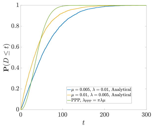
Figure 6: Single turn case from the typical point and the typical intersection.

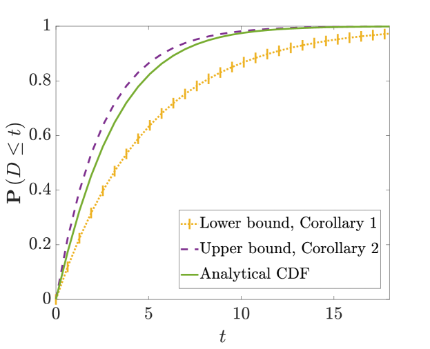
Figure 7: Single turn case from a typical intersection along with the upper and lower bounds.

Fig. 6 shows that the distance to the nearest PLCP point is statistically closer from the nearest intersection as compared to the nearest point due to the two possible initial paths $L_{\rm x}$ and $L_{\rm y}$ available from the typical intersection as compared to only one path available from the typical point. Furthermore, for comparison, we plot the nearest neighbor distribution for a 2D PPP with intensity $\lambda_{\rm PPP}=\mu\lambda$. Interestingly, we see that the CDF is lower for the 2D PPP for lower values of $t$, while the contrary is true for higher values of $t$. Indeed, due to the fact that a line passes through the typical point of a PLCP, the nearest point can likely be present on such a line. Based on the values of $\mu$ and $\lambda$, this may be closer or farther than the nearest neighbor of a 2D PPP with intensity $\mu\lambda$. However, in case the shortest path to a point is present in a different line than the one passing through the typical PLCP point, its Euclidean distance is smaller than the path length.

Fig. 7 demonstrates the upper and the lower bounds for the shortest path length distribution from the typical intersection as compared to the actual value. Recall that the lower bound is obtained by evaluating the void probability of $(\Phi_{\rm x}\cup\Phi_{\rm y})\cap\mathcal{B}(0,t)$, where $\Phi_{\rm x}$ and $\Phi_{\rm y}$ respectively represent the points of $\Phi$ on $L_{\rm x}$ and $L_{\rm y}$. On the contrary, the upper bound follows from the void probability of $(\Phi_{\rm x}\cup\Phi_{\rm y}\cup\Phi_{\rm Ix}\cup\Phi_{\rm Iy})\cap\mathcal{B}(0,t)$, where $\cup\Phi_{\rm Ix}$ and $\cup\Phi_{\rm Iy}$ are the intersection in $\Phi_{\rm I}$ present along $L_{\rm x}$ and $L_{\rm y}$, respectively. Naturally, the lower bound is tighter when $\mu$ is higher while the upper bound is tighter when $\lambda$ is higher. Both the bounds can act as surrogate measures for analysing the performance of wireless networks with low computational complexity. This is discussed further in the next section.

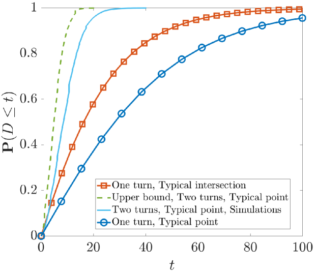
Figure 8: Comparison of the single turn and turn cases from the typical point and the single turn case from a typical intersection

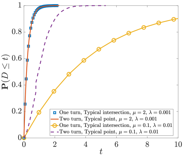
Figure 9: Comparison of the single turn case from the typical intersection with the two turn case from a the typical point for different line and point densities.

Fig. 8 compares the shortest path length distribution from the typical point and the typical intersection for the single turn case with the same from the typical point for the two turn case. For illustration we have also plotted the analytical bound derived in Theorem 3. Naturally, allowing for two turns statistically brings the nearest point of the PLCP closer. However, Fig. 9 shows that based on the line and point densities, the distance to the nearest point may be same for the two turn case form the typical point and the one turn case from the typical intersection. Indeed, while the former has the benefit of having two starting paths, i.e., along $L_{\rm x}$ and $L_{\rm y}$, the later has the advantage of taking two turns, thereby resulting in the same statistics of the shortest path length, especially for high values of $\mu$ and low values of $\lambda$. On the contrary, for high $\lambda$ and/or low $\mu$, the nearest point is much closer to the typical point if two turns are allowed as compared to the typical intersection in case only a single turn is allowed.

VI Applications

VI-A Near-Field Broadcasting of Basic Safety Messages Leveraging RIS

In RF communications, based on electromagnetic principles, the total gain of the cascaded channel (transmitter-RIS-receiver) is approximately the product of the gains from these two sub-channels and the reflection coefficient of the RIS element, characterizing it as a multiplicative channel. In contrast, the channel reflected by an optical re-configurable intelligent surface (ORIS), especially in the near-field and very near-field regime, behaves as an additive channel [16, 17]. This behavior is also observed in the near-field broadcasting configuration of RISs even for RF communications [18]. In such near-field transmission, the reflected signal can thus be considered as emanating directly from a virtual transmitter, which is symmetrically positioned relative to the actual transmitter across the plane of the RIS reflecting element.

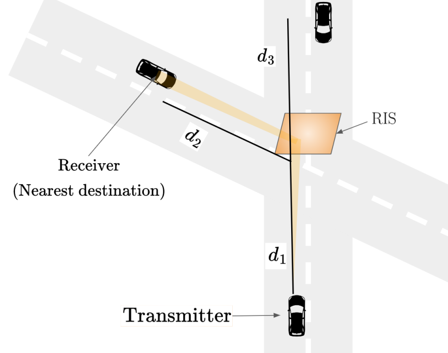
Figure 10: Illustration of V2V communication using ORIS. The transmitter intends to communicate to the vehicle that will experience the strongest received power. This may be a vehicle present in an intersecting street. Due to the specular reflector model, the received power is a function of the path lengths.

Accordingly, consider the V2V communication system shown in Fig. 10 where the vehicles intend to transmit basic safety messagess to neighboring vehicles as they approach street intersections. The vehicles employ a network-configured PC5 side-link to communicate [19]. Assume that RISs are deployed on the street intersections so that the vehicle on intersecting streets can communication with each other. Considering the size of the RIS to be large as compared to the transmitting distance, the transmitter can be assume to be in the near-field of the RIS. For the transmitter, the nearest vehicle (in terms of the path length) may either be on the same street at a distance $d_{1}+d_{3}$ from the transmitter (as illustrated in the figure), or in the intersecting street at a path length $d_{1}+d_{2}$, connected via the RIS. In case the transmitter leverages the RIS to communicate with the receiver located on the intersecting street, the received signal power in the near-field broadcasting regime is approximated as [18]

$$P_{ri}\approx\frac{G_{t}G_{r}\lambda^{2}A^{2}}{16\pi^{2}(d_{1}+d_{i})^{2}}P_{t};\quad i\in\{2,3\},$$ (17)

where $G_{t},G_{r},$ and $P_{t}$ are respectively the transmitter gain, receiver gain, and the transmit power. The carrier wavelength is $\lambda$ and $A$ is the area of the RIS board. Based on the distances of other vehicles, the nearest receiver corresponds to either $i\in\{2,3\}$. Let us assume that the receiver is able to decode the BSM packets if the received signal to noise ratio (SNR) is higher than a threshold $\gamma$. Naturally, for a noise power $N_{0}$, the probability that the nearest vehicle to the transmitter successfully decodes the BSM packet is evaluated as

$$\mathbb{P}\left(\max_{i}\{P_{r}\}\geq\gamma\right) \approx\mathbb{P}\left(\min_{i}\{d_{1}+d_{i}\}\leq\left(\frac{16\pi^{2}\gamma N_{0}}{G_{t}G_{r}\lambda^{2}A^{2}}\right)^{\frac{1}{2}}\right)$$

$$=F_{D}\left(\left(\frac{16\pi^{2}\gamma N_{0}}{G_{t}G_{r}\lambda^{2}A^{2}}\right)^{\frac{1}{2}}\right),$$ (18)

which is evaluated using (1).

VI-B Bound for Far-Field Communications

The shortest path distribution can be used to derive bound on the far-field communication. In particular, the maximum far-field received power with optimized phase responses and no misalignment is given by [18]

$$P_{\text{F}}=\frac{G_{t}G_{r}GM^{2}N^{2}d_{x}d_{y}\lambda^{2}A^{2}}{64\pi^{3}d_{1}^{2}d_{2}^{2}}P_{t},$$ (19)

where $d_{x}$ and $d_{y}$ represent the size of a unit cell along the two dimensions of a square RIS. $M$ and $N$ are respectively the number of RIS elements along the two dimensions. Consequently,

$$\mathbb{P}\left(P_{\text{F}}\geq\gamma\right)=\mathbb{P}\left(\frac{G_{t}G_{r}GM^{2}N^{2}d_{x}d_{y}\lambda^{2}A^{2}}{64\pi^{3}d_{1}^{2}d_{2}^{2}}P_{t}\geq\gamma\right)$$

$$=\mathbb{P}\left(d_{1}d_{2}\leq\sqrt{\frac{64\pi^{3}}{G_{t}G_{r}GM^{2}N^{2}d_{x}d_{y}\lambda^{2}A^{2}}}\right)$$

$$\overset{(a)}{\geq}\mathbb{P}\left(d_{1}+d_{2}\leq 2\left({\frac{64\pi^{3}}{G_{t}G_{r}GM^{2}N^{2}d_{x}d_{y}\lambda^{2}A^{2}}}\right)^{\frac{1}{4}}\right)$$

$$=F_{D}\left(2\left({\frac{64\pi^{3}}{G_{t}G_{r}GM^{2}N^{2}d_{x}d_{y}\lambda^{2}A^{2}}}\right)^{\frac{1}{4}}\right),$$

where the step $(a)$ is is from the inequality that the arithmatic mean of $d_{1}$ and $d_{2}$ is greater than the corresponding geometric mean.

VI-C Transport Infrastructure Modeling

One of the key bottlenecks for the proliferation of electric vehicles is battery capacity, leading to the requirement of high density of deployment of charging points across the streets of a city. Researchers have recently employed tools from stochastic geometry to plan for placement of charging points in a city, e.g., see [20]. However, an accurate study of charging point accessibility needs the characterization of the path-lengths. In this regard, the location of such charging points can be modeled as points of a PLCP, while a typical vehicle can be modeled as the typical point of the PLCP. This framework presents several opportunities for mathematical analysis. For example, the shortest path length distributions characterized in this paper can be leveraged to calculate the distance that the typical vehicle needs to travel in order to find the nearest charging point of a given density of streets and the density of changing points. Similarly, as explained in [20], for urban electric bus networks connected via power lines laid throughout the streets, a disconnected bus can get connected to the grid based on the shortest path lengths between busses. Although the authors in [20] did not explore this analytically, possibly due to the lack of an accurate characterization of path length distributions, the results of this paper may aid in such analysis. Furthermore, expanding on the findings, one can analytically describe distance-based cost metrics relevant to transportation systems, such as minimizing travel time and fuel consumption. These insights could be valuable in assessing the response times of medical or police teams arriving at emergency locations and for budgeting of bus and tram stops in a city.

VII Conclusion and Open Questions

We have derived the shortest path length distribution to a PLCP point from the typical point of a PLCP and the typical intersection of a PLP under the restriction of one turn. Furthermore, we have derived a bound for the shortest path length distribution to a PLCP point from the typical point of a PLCP under the restriction of two turns. Interestingly, for dense point densities and low line densities, the nearest point is closer to the typical intersection restricted to one turn as compared to the same from the typical point restricted to two turns. We highlighted two applications, one on V2V communications using optical links and the other on deployment of electric vehicle charging points, where our derived framework may be employed for statistical analysis.

We are currently investigating the general case, i.e., without a restriction on the number of turns for the shortest path length. Furthermore, percolation questions are open, e.g., what is the probability that there exists an infinitely connected component in terms of the path lengths.

References

- [1] B. Ripley, “The foundations of stochastic geometry,” The Annals of Probability, vol. 4, no. 6, pp. 995–998, 1976.
- [2] F. Baccelli et al., “Stochastic geometry and architecture of communication networks,” Telecommunication Systems, vol. 7, no. 1, pp. 209–227, 1997.
- [3] C.-S. Choi and F. Baccelli, “Poisson Cox point processes for vehicular networks,” IEEE Transactions on Vehicular Technology, vol. 67, no. 10, pp. 10 160–10 165, 2018.
- [4] H. S. Dhillon and V. V. Chetlur, “Poisson line Cox process: Foundations and applications to vehicular networks,” Synthesis Lectures on Learning, Networks, and Algorithms, vol. 1, no. 1, pp. 1–149, 2020.
- [5] J. P. Jeyaraj and M. Haenggi, “Cox models for vehicular networks: SIR performance and equivalence,” IEEE Transactions on Wireless Communications, vol. 20, no. 1, pp. 171–185, 2020.
- [6] J. P. Jeyaraj et al., “The transdimensional Poisson process for vehicular network analysis,” IEEE Transactions on Wireless Communications, vol. 20, no. 12, pp. 8023–8038, 2021.
- [7] G. Ghatak, “Binomial line processes: Distance distributions,” IEEE Transactions on Vehicular Technology, vol. 71, no. 2, pp. 2176–2180, 2021.
- [8] G. Ghatak et al., “Small cell deployment along roads: Coverage analysis and slice-aware RAT selection,” IEEE Transactions on Communications, vol. 67, no. 8, pp. 5875–5891, 2019.
- [9] F. Morlot, “A population model based on a Poisson line tessellation,” in 2012 10th International Symposium on Modeling and Optimization in Mobile, Ad Hoc and Wireless Networks (WiOpt), 2012, pp. 337–342.
- [10] V. V. Chetlur, H. S. Dhillon, and C. P. Dettmann, “Shortest path distance in Manhattan Poisson line Cox process,” Journal of Statistical Physics, vol. 181, pp. 2109–2130, 2020.
- [11] D. M. Nguyen, M. A. Kishk, and M.-S. Alouini, “Modeling and analysis of dynamic charging for EVs: A stochastic geometry approach,” IEEE Open Journal of Vehicular Technology, vol. 2, pp. 17–44, 2020.
- [12] C. Gloaguen et al., “Analysis of shortest paths and subscriber line lengths in telecommunication access networks,” Networks and Spatial Economics, vol. 10, no. 1, pp. 15–47, 2010.
- [13] N. Miyoshi, “Neveu’s exchange formula for analysis of wireless networks with hotspot clusters,” Frontiers in Communications and Networks, vol. 3, p. 885749, 2022.
- [14] F. Voss, C. Gloaguen, and V. Schmidt, “Scaling limits for shortest path lengths along the edges of stationary tessellations,” Advances in Applied Probability, vol. 42, no. 4, pp. 936–952, 2010.
- [15] S. N. Chiu, D. Stoyan, W. S. Kendall, and J. Mecke, Stochastic geometry and its applications. John Wiley & Sons, 2013.
- [16] S. Sun et al., “Optical intelligent reflecting surface assisted MIMO VLC: Channel modeling and capacity characterization,” IEEE Transactions on Wireless Communications, 2023.
- [17] ——, “Optical IRS for Visible Light Communication: Modeling, Design, and Open Issues,” arXiv preprint arXiv:2405.18844, 2024.
- [18] W. Tang, M. Z. Chen, X. Chen, J. Y. Dai, Y. Han, M. Di Renzo, Y. Zeng, S. Jin, Q. Cheng, and T. J. Cui, “Wireless communications with reconfigurable intelligent surface: Path loss modeling and experimental measurement,” IEEE transactions on wireless communications, vol. 20, no. 1, pp. 421–439, 2020.
- [19] R. Molina-Masegosa, J. Gozalvez, and M. Sepulcre, “Configuration of the C-V2X mode 4 sidelink PC5 interface for vehicular communication,” in 2018 14th International conference on mobile ad-hoc and sensor networks (MSN). IEEE, 2018, pp. 43–48.
- [20] R. Atat, M. Ismail, and E. Serpedin, “Stochastic geometry planning of electric vehicles charging stations,” in ICASSP 2020-2020 IEEE International Conference on Acoustics, Speech and Signal Processing (ICASSP). IEEE, 2020, pp. 3062–3066.