The perfomance of generalized Davies-Cotton optical systems with infinitesimal mirror facets.

Abstract

This paper presents Taylor expansions for the imaging and timing characteristics of spherical optical systems with infinitesimal mirror facets, sometimes referred to as “modified Davies-Cotton” telescopes. Such a system comprises a discontinuous spherical mirror surface whose curvature radius is different from its focal length, and whose mirrors are aligned to suppress spherical aberration. Configurations that range between two “optima” are, one of which minimises tangential comatic aberration and the other that minimises timing dispersion.

1 Introduction

In Section 2 of Vassiliev et al. (2007, hereafter VFB) we presented an expression for the first and second moments of the light distribution formed by parallel rays reflected from an “ideal” Davies-Cotton telescope (Davies and Cotton, 1957, DC), i.e. one with infinitesimal facets, neglecting diffraction. Our expression consisted of a Taylor expansion in leading orders of the off-axis field angle, $\delta$, and in $\frac{1}{4f^{2}}$, where $f=F/D$ is the ratio of the focal distance, $F$, to the diameter of the aperture, $D$. We discussed the leading order terms expansion for the tangential and sagittal second moments, spherical aberration ($\propto\delta^{0}/f^{6}$), coma ($\propto\delta^{2}/f^{4}$) and astigmatism ($\propto\delta^{4}/f^{2}$), and also considered the effects of focal-plane curvature. Additional terms in the leading-order expansion were subsequently given by Bretz and Ribordy (2013, hereafter BR). Schliesser and Mirzoyan (2005, hereafter SM) provided third-order expressions for continuous mirrors in the form of conics of rotation, which cover parabolic, spherical, and elliptical mirrors. Such analytic approximations are generally useful, for example to (1) quickly evaluate the performance of tessellated optical systems, neglecting aberrations from the finite facet size, and (2) validate DC ray-tracing simulation codes.

In VHE gamma-ray astronomy with imaging atmospheric Čerenkov telescopes (IACTs) such simulation codes are often part of the Monte-Carlo simulation chain from which the performance of the IACT instrument is calculated. For performance reasons, such codes are not usually based on general-purpose ray-tracing packages, rather they are custom-developed codes optimised for DC-like telescopes. Expansions such as those in VFB and BR could be used to validate such codes by simulating telescopes with a large number of small (but finite) mirror facets. However, these expressions apply to the case of a telescope with infinitesimal mirrors arranged in such a way that all incoming rays are reflected to the focus irrespective of field angle, whereas most DC telescopes that have been built, and most simulation codes, assume identical mirror facets arranged on a regular grid perpendicular to the optic axis, e.g. hexagonal or square. These facets cannot all be aligned perpendicular to the incoming rays and hence some rays will not be reflected, passing through “the cracks” between mirrors that arise due to this non-perpendularity, giving a small but significant difference between the analytic expressions and the limiting case from the simulations.

Some recent IACTs, such as the medium-sized telescopes (Garczarczyk et al., 2015, MST) of the Čerenkov telescope array (CTA), deviate from the classical DC design in which the curvature radius of the spherical dish, $R$, equals the focal distance. The response of such generalised DC telescopes, and those that have a parabolic dish design, cannot be approximated with the expressions of VFB. The expressions of SM apply to continuous mirror systems intermediate between spherical and paraboloid, however these systems have significantly worse optical performance than that of the discontinuous generalised DC system, except in the parabolic case.

The following section presents expressions for the performance of a general spherical telescope with infinitesimal mirror facets laid out on a regular grid, which can be used for design studies and to validate ray-tracing simulations with small mirror facets. Since the methodology is very similar to that of VFB, only differences between the analyses are presented in detail.

2 Taylor series expansions

Adopting the notation of Section 2 of VFB, the surface of the primary mirror is $\vec{r}(\varphi,\theta)=R(\sin\theta\cos\phi,\sin\theta\sin\phi,1-\cos\theta)$, with $\theta\in[0,\sin^{-1}(D/2R)]$ and $\varphi\in[0,2\pi]$. For a general spherical telescope there is no global alignment point; instead to focus parallel on-axis rays to a point at $\vec{r_{F}}=(0,0,F)$ each facet must be aligned to a point on the z-axis the same distance from the focal point as is the facet, $\vec{r_{A}}=(0,0,z_{A})$ with,

$$z_{A}=F+|\vec{r}(\phi,\theta)-\vec{r_{F}}|=F+\sqrt{4R(R-F)\sin^{2}(\theta/2)+F^{2}}.$$ (1)

The normal for each facet is then $\vec{n}(\varphi,\theta)=\frac{\vec{r_{A}}-\vec{r}(\varphi,\theta)}{|\vec{r_{A}}-\vec{r}(\varphi,\theta)|}$. As in VFB the direction of the incoming parallel rays is written as $\vec{g}=(\sin\delta,0,-\cos\delta)$, and the direction of the reflected ray as $\vec{u}(\varphi,\theta)=\vec{g}-2\left(\vec{g}\cdot\vec{n}(\varphi,\theta)\right)\vec{n}(\varphi,\theta)$. The path of the reflected ray is from the mirror to the focal plane can be parameterised by $s$ as, $\vec{r}_{ray}(s;\varphi,\theta)=\left(x_{ray}(s),y_{ray}(s),z_{ray}(s)\right)=\vec{r}(\varphi,\theta)+s\vec{u}(\varphi,\theta)$, from which the propagation distance from the mirror to the focal plane, $s_{fp}(\varphi,\theta)$, can be found by solving $z_{ray}(s_{fp})=F$, where a curved focal plane is not considered. The coordinates of the ray on the focal plane are then $x_{fp}(\varphi,\theta)=x_{ray}(s_{fp}(\varphi,\theta);\varphi,\theta)$ and $y_{fp}(\varphi,\theta)=y_{ray}(s_{fp}(\varphi,\theta);\varphi,\theta)$.

Calculation the moments of the distribution of rays on the focal plane is achieved by integrating the appropriate function over the infinitesimal mirrors of surface area $\mathrm{d}S=R^{2}\cos\theta\sin\theta\mathrm{d}\theta\mathrm{d}\phi$. Each mirror facet presents an area of $|\vec{g}\cdot\vec{n}(\varphi,\theta)|\mathrm{d}S$ to the incoming rays, which are reflected to the focal plane, assuming no obscuration. The moments are then calculated using the functional,

$$\mathcal{I}[f(\varphi,\theta)]=\int_{0}^{\sin^{-1}(D/2R)}\int_{0}^{2\pi}f(\varphi,\theta)|\vec{g}\cdot\vec{n}(\varphi,\theta)|R^{2}\cos\theta\sin\theta\mathrm{d}\theta\mathrm{d}\phi,$$ (2)

where the inclusion of the dot-product term represents the second difference between this analysis and that of VFB.

The effective area of the telescope for rays is given by $A=\mathcal{I}[1]$. The first moments of the light distribution are then $\langle x\rangle=\mathcal{I}[x_{fp}]/A$ and $\langle y\rangle=\mathcal{I}[y_{fp}]/A$. The centered second order moments are $\langle\Delta x^{2}\rangle=\mathcal{I}[x_{fp}^{2}]/A-\langle x\rangle^{2}$, $\langle\Delta y^{2}\rangle=\mathcal{I}[y_{fp}^{2}]/A-\langle y\rangle^{2}$, and $\langle\Delta x\Delta y\rangle=\mathcal{I}[x_{fp}y_{fp}]/A-\langle x\rangle\langle y\rangle$. Writing the propagation time of the rays through the system with respect to an arbitrary offset as,

$$t_{fp}(\varphi,\theta)=\frac{s_{fp}(\varphi,\theta)+\vec{g}\cdot\vec{r}(\varphi,\theta)}{\mathrm{c/n}},$$

where $\mathrm{c/n}$ is the speed of light in the air, the variance of the distribution of arrival times on the focal plane can be expressed as $\langle\Delta t^{2}\rangle=\mathcal{I}[t_{fp}^{2}]/A-\mathcal{I}[t_{fp}]^{2}/A^{2}$.

As in VFB the integrals are computed and, with the exception of $A$, the results expressed as Taylor expansions in leading orders of $\delta$ and $\frac{1}{4f^{2}}$. For convenience the results are expressed in terms of the ratio of the focal distance to reflector radius, $\mathpzc{c}=F/R$. For the classic DC telescope, $\mathpzc{c}=1$; a good approximation to a parabolic reflector can be made with $\mathpzc{c}=1/2$; the CTA MST corresponds to $\mathpzc{c}=16/19.2=0.83$ (and $f=16/12=1.33$, Garczarczyk et al., 2015).

In the case of $A$ the dependency on $\delta$ can be expressed fully, so the Taylor expansion is done only in terms of $\frac{1}{4f^{2}}$,

$$A=\pi\left(\frac{D}{2}\right)^{2}\left(1-\frac{1}{64f^{2}}-\frac{16\mathpzc{c}-11}{6144f^{4}}\right)\cos\delta.$$ (3)

This is smaller than the canonical value of $\pi\left(\frac{D}{2}\right)^{2}\cos\delta$ by $1.6\%/f^{2}$ to leading order, showing that with this mirror configuration rays are lost even in the “ideal” case of an infinite number of identical infinitesimal facets on a grid.

The centroids of the light distribution on the focal plane are,

$$\frac{\langle x\rangle}{F}=\,\delta\left(1+\frac{3-2\mathpzc{c}}{32f^{2}}+\frac{-16\mathpzc{c}^{3}+50\mathpzc{c}-11}{6144f^{4}}\right)+\frac{\delta^{3}}{3}\left(1+\frac{3-\mathpzc{c}}{16f^{2}}\right)$$ (4)

and $\frac{\langle y\rangle}{F}=0$, from which it is evident that there is a leading-order plate-scale correction of $(3-2\mathpzc{c})/32f^{2}$. This amounts to a correction of $3.1\%/f^{2}$ for the classic DC design, $6.3\%/f^{2}$ for a parabolic mirror. In the case of $\mathpzc{c}=3/2$, i.e. a system with $R=2F/3$, the first order plate-scale correction is eliminated.

The centered second order moments in the tangential ($x$) and sagittal ($y$) directions are,

$$\frac{\langle\Delta x^{2}\rangle}{F^{2}} =\frac{\delta^{2}}{1024f^{4}}\left(\frac{4\mathpzc{c}^{2}-12\mathpzc{c}+11}{3}+\frac{32\mathpzc{c}^{4}-48\mathpzc{c}^{3}-96\mathpzc{c}^{2}+184\mathpzc{c}-13}{192f^{2}}\right.$$

$$\quad\quad\left.+\frac{2240\mathpzc{c}^{6}-2592\mathpzc{c}^{5}-5696\mathpzc{c}^{4}-224\mathpzc{c}^{3}+17026\mathpzc{c}^{2}-4626\mathpzc{c}+1119}{92160f^{4}}\right)$$

$$+\frac{\delta^{4}}{16f^{2}}\left(1+\frac{8\mathpzc{c}^{2}-36\mathpzc{c}+217}{576f^{2}}+\frac{32\mathpzc{c}^{4}-72\mathpzc{c}^{3}-144\mathpzc{c}^{2}+1276\mathpzc{c}+629}{18432f^{4}}\right)$$

$$+\frac{\delta^{6}}{12f^{2}}\left(1+\frac{17\mathpzc{c}^{2}-111\mathpzc{c}+1528}{2880f^{2}}\right),$$ (5)

$$\frac{\langle\Delta y^{2}\rangle}{F^{2}} =\frac{\delta^{2}}{1024f^{4}}\left(\frac{2}{3}+\frac{24\mathpzc{c}+11}{192f^{2}}+\frac{1152\mathpzc{c}^{3}+3456\mathpzc{c}^{2}+4136\mathpzc{c}-811}{184320f^{4}}\right)$$

$$+\frac{\delta^{4}}{2304f^{4}}\left(1+\frac{24\mathpzc{c}+47}{128f^{2}}+\frac{1152\mathpzc{c}^{3}+3456\mathpzc{c}^{2}+17960\mathpzc{c}+3185}{122880f^{4}}\right)$$

$$+\frac{17\delta^{6}}{69120f^{4}}\left(1+\frac{408\mathpzc{c}+1627}{2176f^{2}}\right),$$ (6)

while the covariance term is zero, $\frac{\langle\Delta x\Delta y\rangle}{F^{2}}=0$. We note that spherical aberration ($\propto\delta^{0}/f^{6}$) is suppressed for all values of $\mathpzc{c}$, by construction. The leading order aberration is coma ($\propto\delta^{2}/f^{4}$). In the expression for the tangential coma, the first sub-term (i.e. quadratic in $\mathpzc{c}$) is twice as large in the parabolic reflector case ($2$ for $\mathpzc{c}=1/2$) as it is in the DC case ($1$ for $\mathpzc{c}=1$). This term is minimised by $\mathpzc{c}=3/2$, the same value that was found to eliminate the plate-scale correction above, for which the term is $2/3$. The second sub-term of the tangential coma expression (the fourth order polynomial $\propto\delta^{2}/f^{6}$) is also close to its minimum at $\mathpzc{c}=3/2$ (the minimum is at $\mathpzc{c}=1.48$). In fact, for $\mathpzc{c}=3/2$ the tangential and sagittal coma expressions are the same to two leading orders, both equalling $\frac{\delta^{2}}{1024f^{4}}\left(\frac{2}{3}+\frac{47}{192f^{2}}\right)$. However, the tangential astigmatism term is significantly larger than the sagittal, which means that $\frac{\langle\Delta x^{2}\rangle}{F^{2}}\gg\frac{\langle\Delta y^{2}\rangle}{F^{2}}$ for $\delta\gg 0$, even for $\mathpzc{c}=3/2$.

The variance in the distribution of ray impact times on the focal plane is,

$$\langle\Delta t^{2}\rangle =\left(\frac{D}{\mathrm{c}/\mathrm{n}}\right)^{2}\left\{\frac{1}{768f^{2}}\left((2\mathpzc{c}-1)^{2}+\frac{(2\mathpzc{c}-1)(2\mathpzc{c}^{3}-2\mathpzc{c}+1)}{8f^{2}}\right.\right.$$

$$\quad\left.+\frac{4480\mathpzc{c}^{6}-1728\mathpzc{c}^{5}-3840\mathpzc{c}^{4}-1664\mathpzc{c}^{3}+8196\mathpzc{c}^{2}-5508\mathpzc{c}+1153}{61440f^{4}}\right)$$

$$-\left.\frac{\delta^{2}}{256f^{2}}\left(2\mathpzc{c}-1+\frac{3\mathpzc{c}^{3}+6\mathpzc{c}^{2}-5\mathpzc{c}-2}{24f^{2}}\right)\right\},$$ (7)

which is, in general, non-zero even for $\delta=0$. A parabolic mirror is well known to be isochronous for rays parallel to the optic axis; for the spherical approximation, with $\mathpzc{c}=1/2$, the first two terms of $\delta=0$ are identically zero, but the third term, of order $\frac{1}{f^{6}}$, is marginally non-zero. To get an idea of the relative size of the $\delta^{0}$ and $\delta^{2}$ terms, keeping only the leading orders in $\frac{1}{4f^{2}}$, the RMS of the impact time distribution for $\mathpzc{c}>1/2$ can be approximated as,

$$\sigma_{t}=\sqrt{\langle\Delta t^{2}\rangle}\approx\frac{D}{10\,\mathrm{m}}\,\frac{\mathrm{n}}{f}\left\{1.2036\,(2\mathpzc{c}-1)-0.00055\,\left(\frac{\delta}{1\,\mathrm{deg}}\right)^{2}\right\}\,\mathrm{ns},$$ (8)

from which it is evident that the dependency on field angle is small compared to the constant term, except for the configurations close to parabolic, $\mathpzc{c}\approx 1/2$, where higher order terms dominate. The classic DC design ($\mathpzc{c}=1$) has a characteristic dispersion of $\sigma_{t}\approx 1.2/f$ ns for a $10$ m telescope, whereas for the case of the “minimal coma” solution with $\mathpzc{c}=3/2$ the time dispersion is twice as large. For the case of $\mathpzc{c}=1/2$ the spherical approximation to a parabolic reflector has a leading-order time dispersion of,

$$\sigma_{t}\approx 0.019\frac{D}{10\,\mathrm{m}}\frac{\mathrm{n}}{f^{3}}\sqrt{1+0.38f^{2}\left(\frac{\delta}{1\,\mathrm{deg}}\right)^{2}}\,\mathrm{ns}.$$

Finally, the configuration with planar mirror surface, $\mathpzc{c}=0$, has a time dispersion that is no worse that the DC, but the RMS of the tangential coma is twice as large as the DC case. Large planar mirror systems are used as solar collectors, but it seems unlikely that the configuration provides a compelling advantage for applications in large imaging telescopes. However, the solution is a close analogue of the Fresnel lens, which is a flat, discontinuous, refractive focussing element that has proven useful and cost-effective on smaller scales. A reflective equivalent would resemble a negative-curvature (diverging) Fresnel lens with a reflective coating. The curvature on each of the grooves would be significantly less than for a lens of equal focal length, and the same diamond-turning or 3D-printing technology could be used to form the surface. In wideband imaging applications, such as Čerenkov astronomy, such a reflector may provide advantages over a Fresnel lens, whose imaging quality is limited by chromatic aberrations.

3 Accuracy

Figure 1 shows a comparison between the Taylor expansions given above and the results from numerically integrating Equation 2 to high accuracy, for field angles of $\delta<10^{\circ}$. The calculation assumes a system with $D=10$ m, $F=12$ m, and three values for the curvature radius, $R=\{8,12,24\}$ m, indicated as $\mathpzc{c}=F/R=\{3/2,1,1/2\}$ respectively on the plots. The three plots correspond to: image centroid, Equation 4 (left); tangential and sagittal image RMS, Equations 5 and 6 (middle); and arrival time dispersion, Equation 7 (right).

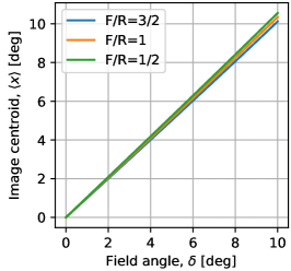
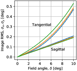
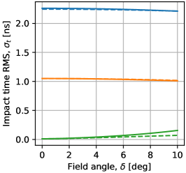
Figure 1: Comparison between Taylor series expressions (dashed lines) and results from quadrature numerical integration (solid lines) for: image centroid (left); tangential and sagittal image RMS (middle); and arrival time dispersion (right).

The accuracy of the Taylor expansions depend on $f$, $\mathpzc{c}$, and $\delta$, but for the cases presented here, all are accurate to better than $1\%$ with the following two exceptions: (1) for $\mathpzc{c}=3/2$ the error in $\sigma_{x}$ and $\sigma_{y}$ rise to 1.04% at $\delta=10^{\circ}$, and (2) for $\mathpzc{c}=1/2$ the error in $\sigma_{t}$ is $>$50% at $\delta=10^{\circ}$. These cases correspond to the optima for the imaging and time resolution, where the low-order terms are minimised, and for which higher-order terms become more important, and it is therefore not surprising that they do not perform well. The Taylor expansion for $\sigma_{t}$ does not converge quickly and a large number of additional terms in $\delta$ and $\frac{1}{4f^{2}}$ would be required to achieve the same accuracy as the other expansions presented here. If greater accuracy is required for any of the expressions discussed here a Python notebook that numerically integrates Equation 2 is included in the online material. The notebook also contains Python functions that implement Equations 4–7.

4 Discussion

An analysis of the general case of spherical optical system with “identical” regularly-spaced infinitesimal mirror facets has been presented. The expressions differ that those presented before in two ways: (1) generalizing the classical DC constraint that the curvature radius and focal length are equal, and (2) accounting for light loss around the edges of the facets whose normals are not in general aligned with the rays. In addition to presenting expressions for the moments of the image on the focal plane, expansions for the effective area, which accounts for light losses, and the dispersion of the distribution of propagation times through the system have been presented.

In the case of a pure DC design these new expansions differ to some degree from those of VFB (as corrected by BR), due to the effect of the rays lost at the facet edges. For example, with $\mathpzc{c}=1$ Equation 5 can be approximated as, $\frac{\langle\Delta x^{2}\rangle}{F^{2}}=\frac{\delta^{2}}{1024f^{4}}\left(1+\frac{0.3073}{f^{2}}\right)+\frac{\delta^{4}}{16f^{2}}\left(1+\frac{0.3264}{f^{2}}\right)$, while the equivalent expression from VFB is, $\frac{\langle\Delta x^{2}\rangle}{F^{2}}=\frac{\delta^{2}}{1024f^{4}}\left(1+\frac{0.3125}{f^{2}}\right)+\frac{\delta^{4}}{16f^{2}}\left(1+\frac{0.3646}{f^{2}}\right)$. For the parabolic case, Equation 5 (with $\mathpzc{c}=1/2$) agrees with that of SM to the leading orders that they provide, both equalling $\frac{\langle\Delta x^{2}\rangle}{F^{2}}=\frac{\delta^{2}}{512f^{2}}+\frac{\delta^{4}}{16f^{2}}$.

Writing the focal length as $F$ and the radius of curvature of the mirror sphere as $R$, two privileged configurations are identified: $R=2/3F$ for which the tangential coma term is minimised and equals the sagittal coma; and $R=2F$ which minimises (largely eliminates) time dispersion, this latter giving a close approximation to the parabolic surface.

The ratio $\mathpzc{c}=F/R$ can therefore be used to trade off-axis imaging resolution against time dispersion, by varying between the two optima of $\mathpzc{c}=1/2$ and $\mathpzc{c}=3/2$. Using simulations of tessellated mirror systems SM discuss the same trade-off and suggest an elliptical system with $R=0.85F$ as one of interest. For the CTA MST a system with $R=1.2F$ was chosen to improve the time resolution at the cost of slightly degraded imaging resolution (Garczarczyk et al., 2015).

The cost of a DC-like telescope is largely determined by the size of the aperture, $D$, which determines the total mirror surface area, and the focal length, which determines the size of the camera and the cost of the structure required to support it. The cost associated with changing the curvature radius from the DC case of $R=F$ comes from (1) accommodating a larger maximum sag (if $R<F$), and (2) having mirror facets with different optimal focal distances. The maximal sag for a telescope of diameter $D$ is approximately $z_{max}\approx\frac{D^{2}}{8R}$. For example, for a system with $D=10$ m and $F=12$ m this amounts to $z_{max}=1.09$ m for the DC case ($R=12$ m), $z_{max}=0.53$ m for the parabolic case ($R=24$ m), and $z_{max}=1.76$ m for the minimum coma configuration ($R=8$ m). The difference in cost of the structures with this range of maximum sag, $(0.53,1.76)$ m, is likely small compared to the total cost of the system; this parameter can be used to tune the performance of the system without impacting the cost excessively.

This note does not study the effects of finite mirror facet size. The size of these effects depends primarily on the facet $f$-number, which is usually quite large, the surface quality of the facets, the distribution of focal lengths across the support structure, and deformations of the structure as it moves. The shape and layout of the facets on the telescope play secondary roles. The phase space for these effects is therefore large and there is no simple equation to describe the combined PSF from a faceted telescope, although BR provide reasonable fits to simulations in the DC case. Ray-tracing simulations are generally required to calculate the detailed response of the system.

References

- Bretz and Ribordy (2013) Bretz, T., Ribordy, M., 2013. Design constraints on Cherenkov telescopes with Davies-Cotton reflectors. Astropart. Phys. 45, 44–55. doi:10.1016/j.astropartphys.2013.03.004.
- Davies and Cotton (1957) Davies, J., Cotton, E., 1957. Design of the quartermaster solar furnace. Journal of Solar Energy, Science and Engineering 1, 16–22.
- Fazio et al. (1968) Fazio, G.G., Helmken, H.F., Rieke, G.H., Weekes, T.C., 1968. An experiment to search for discrete sources of cosmic gamma rays in the to eV region. Canadian Journal of Physics 46, S451–S455.
- Garczarczyk et al. (2015) Garczarczyk, M., et al., 2015. Status of the Medium-Sized Telescope for the Cherenkov Telescope Array, in: Proc. 34th International Cosmic Ray Conference (ICRC2015).
- Schliesser and Mirzoyan (2005) Schliesser, A., Mirzoyan, R., 2005. Wide-field prime-focus imaging atmospheric Cherenkov telescopes: A systematic study. Astropart. Phys. 24, 382–390. doi:10.1016/j.astropartphys.2005.08.003, arXiv:astro-ph/0507617.
- Vassiliev et al. (2007) Vassiliev, V., Fegan, S., Brousseau, P., 2007. Wide field aplanatic two-mirror telescopes for ground-based gamma-ray astronomy. Astropart. Phys. 28, 10–27. doi:10.1016/j.astropartphys.2007.04.002.