Kibble-Zurek scaling law in dissipative critical dynamics

Abstract

We investigate the dissipative quench dynamics in a family of two-band fermionic systems on bipartite lattices ramped across their critical points, which is cast into the Lindblad formalism. First, we demonstrate an exact solution in the presence of uniform loss or gain, which tells that dissipation exponentially suppresses the Kibble-Zurek (KZ) scaling behavior and the quantum jump part of the dissipation is responsible for the anti-KZ (AKZ) behavior. Then, in a scenario of engineered dissipation, we exemplify the effect of loss difference between the two sublattices of the system by three typical models. By the one-dimensional Rice-Mele model, we unravel a kind of dissipative KZ (DKZ) scaling law in the limit of loss difference and point out a convenient way to observe the DKZ behavior by counting the number of residual particles. Nevertheless, in the one-dimensional Shockley model, we find a nonuniversal scaling behavior irrelevant to the critical dynamics. Thus we explore several quench protocols so that these two scaling behaviors can appear together or separately. At last, we extend our findings to the two-dimensional Haldane model for Chern insulators consistently.

I Introduction

The concepts in equilibrium physics, such as phase transition, critical exponent, and universality, may play an important role in out-of-equilibrium situations [1]. As a cornerstone, the Kibble-Zurek Mechanism (KZM) provides valuable insight in bridging the gap between nonequilibrium critical dynamics and equilibrium criticality [2, 3]. The key aspect of KZM is the frozen effect during the impulse stage of the dynamics [4, 5, 6, 7, 8, 9, 10, 11, 12]. Recently, KZM has been employed as a tool to study the topological insulators through topological quantum phase transitions [13, 14, 15, 16]. Significant progress has been made in developing techniques to generate artificial magnetic fields and spin-orbit coupling for neutral atoms in optical lattices, potentially facilitating the realization and characterization of out-of-equilibrium topological insulator in cold atomic systems [17, 18].

Dissipation may fundamentally influence the critical behaviors of systems or notoriously hinder the probing of them [19]. An intriguing phenomenon termed anti-KZ (AKZ) behavior was observed in ferroelectric phase transitions, in which slower driving results in more defects and covers up the KZ behavior [20]. An explanation is examined in quantum system subjected to a noisy control field [21, 22, 23, 24, 25]. For open systems, the dissipative quench dynamics can be cast into the formalism of Lindblad master equation and has been extensively explored [21, 26, 27, 28, 29, 30, 31, 32, 33, 34].

Nowadays, the impressive experimental advances have enabled the creation of highly controllable environment for studying the emergence of dissipative dynamics in superconducting resonator lattices [35, 36], Rydberg atoms in optical lattices [37], and optomechanical systems [38, 39]. Furthermore, the scenario of engineered dissipation offers a broad prospect. Experiments show it can relax the system of interest to a desired quantum state [40, 41]. More recent experiments have realized the loss difference between two hyperfine states [42] or two sublattices on a photonic lattices [43]. Motivated by these improvements, we demonstrate how a new kind of KZ scaling law could be observed.

II Lindblad equation

In this Letter, we focus on dissipative critical dynamics in both one- and two-dimensional two-band models on bipartite lattices. Assuming that the systems are initially prepared in the ground state far from the critical point and subjected to a linear driving in the presence of dissipation, we put the issue into the Lindblad equation [26, 28],

$$\dot{\rho}=-i[H,\rho]+\sum_{j}\sum_{s}(L_{s,j}\rho L_{s,j}^{\dagger}-\frac{1}{2}\{\rho,L_{s,j}^{\dagger}L_{s,j}\}),$$ (1)

where the summations are over the units ($j$) and sublattices ($s=a,b$), $\rho$ denotes the density operator of the system, $H=H_{t}+H_{u}$ is a fermionic Hamiltonian with the hopping energy $H_{t}=\sum_{j,j^{\prime}}\sum_{s,s^{\prime}}t_{jj^{\prime}}^{ss^{\prime}}c_{s,j}^{\dagger}c_{s^{\prime},j^{\prime}}$ and the on-site energy $H_{u}=u\sum_{j}(c_{a,j}^{\dagger}c_{a,j}-c_{b,j}^{\dagger}c_{b,j})$, $c_{s,j}^{(\dagger)}$ denotes the annihilation (creation) operator, and $L_{s,j}$ represents the jump operator associated with some kind of dissipations. We shall mainly elaborate on the configuration of loss dissipations by setting $L_{a,j}=\sqrt{\gamma_{a}}c_{a,j}$ and $L_{b,j}=\sqrt{\gamma_{b}}c_{b,j}$, where $\gamma_{a}$ and $\gamma_{b}$ are strengths of dissipations on $a$ and $b$ sublattices respectively. The linear driving is implemented through the on-site energy parameter,

$$u=u(t)=u_{i}-\frac{t}{\tau_{Q}}~{}~{}~{}(0\leq t\leq t_{f}),$$ (2)

where the $\tau_{Q}$ is the quench time. The on-site energy parameter is linearly ramped across the quantum phase transition point $u_{c}$ satisfying $u_{i}\geq u_{c}\geq u_{f}=u(t_{f})$.

Without loss of generality, we discuss in one dimension here. It is not hard to generalize the discussion to higher dimension. By a Fourier transition, $c_{a(b),q}=\sum_{j}\frac{e^{-iq\cdot R_{j}}}{\sqrt{N}}c_{a(b),j}$ where $N$ is the total number of units and $R_{j}$ denotes the Bravis lattices, we can reformulate the Hamiltonian in momentum space as $H=\sum_{q}\textbf{d}(q)\cdot\sigma$, where $\sigma=(\sigma_{x},\sigma_{y},\sigma_{z})$ and the components of the vector $\textbf{d}(q)=(d^{x}_{q},d^{y}_{q},d^{z}_{q})$. The exact expressions of the components for specific models will be presented later. The diagonalized Hamiltonian reads $H=\sum_{q}\omega_{q}(\eta_{1,q}^{\dagger}\eta_{1,q}-\eta_{2,q}^{\dagger}\eta_{2,q})$, where the spectrum $\omega_{q}=|\textbf{d}(q)|$ exhibits a gapless point at the critical point $u_{c}$ with critical mode $q_{c}$, the quasiparticle operators $\eta_{1,q}=u_{q}c_{a,q}+v_{q}c_{b,q}$ and $\eta_{2,q}=-v_{q}^{*}c_{a,q}+u_{q}^{*}c_{b,q}$ with Bogoliubov coefficients $\left(u_{q},v_{q}\right)\propto\left(\omega_{q}+d^{z}_{q},d^{x}_{q}-id^{y}_{q}\right)$. The ground state is denoted as $|GS\rangle=\prod_{q}\eta_{2,q}^{\dagger}|0\rangle$, satisfying $c_{a,q}|GS\rangle=c_{b,q}|GS\rangle=0$.

In the Lindblad equation in Eq. (1), the full density matrix $\rho$ can be decomposed into sectors labelled by momentum $q$, so it can be expressed as $\rho=\prod_{q}\bigotimes\rho_{q}$. In each sector, the dimension of the density matrix $\rho_{q}$ reads $4\times 4$, but it contains only 6 nonzero elements including $\rho_{q}^{(11)}$, $\rho_{q}^{(22)}$, $\rho_{q}^{(33)}$, $\rho_{q}^{(44)}$, $\rho_{q}^{(23)}$, and $\rho_{q}^{(32)}$ in the Hilbert space spanned by the base vectors $\{|0\rangle$, $c_{a,q}^{\dagger}|0\rangle$, $c_{b,q}^{\dagger}|0\rangle$, $c_{a,q}^{\dagger}c_{b,q}^{\dagger}|0\rangle\}$. Given that all the elements are worked out, we can deduce the dynamical density of excitations by

$$n(t)=\frac{1}{N}\sum_{q}p_{q}(t),$$ (3)

where the excitation probability $p_{q}(t)=\frac{1}{2}\text{Tr}(\rho\eta_{1,q}^{\dagger}\eta_{1,q})+\frac{1}{2}\text{Tr}[\rho(1-\eta_{2,q}^{\dagger}\eta_{2,q})]$.

Let us define a variable, $R_{q}=\rho_{q}^{(33)}-\rho_{q}^{(22)}$, fulfilling the equation,

$$\frac{\text{d}\tilde{R}_{q}}{\text{d}x} = \frac{\delta}{2}+\frac{\delta^{2}}{4}\int_{x_{0}}^{x}\tilde{R}_{q}(x^{\prime})dx^{\prime}$$ (4)

$$- 4|\Delta_{q}|^{2}\int_{x_{0}}^{x}\tilde{R}_{q}(x^{\prime})\cos\left(\frac{x^{2}-(x^{\prime})^{2}}{\tau_{Q}}\right)dx^{\prime},~{}~{}$$

where $x=t+x_{0}$, $x_{0}=-u_{i}\tau_{Q}$, $\tilde{R}_{q}=e^{\gamma t/2}R_{q}$, $\delta=\gamma_{a}-\gamma_{b}$, and $\Delta_{q}=d^{x}_{q}+id^{y}_{q}$. The initial condition reads $\tilde{R}_{q}(0)=R_{q}(0)=1$, which means half filling of fermions and all of them reside on $b$ sublattice initially since the protocol demands $u_{i}\gg 0$. The solution of this equation is the key to all the 6 nonzero elements.

III Exact solution and AKZ behavior

The Lindblad equation can be solved numerically. However, we seek for an analytical solution. Firstly, if there is no dissipation at all, the first two terms in Eq. (4) disappear. So we get a reduced equation that provides exact solution expressed by the cosine and sine Fresnel’s integrals [44, 45]. For slow quench, we can arrive at the asymptotic solution [46],

$$R_{q}=2e^{-\pi\tau_{Q}|\Delta_{q}|^{2}}+2|u_{q}|^{2}-1~{}~{}~{}(\gamma=\delta=0).$$ (5)

And by Eq. (3), the final excitation density after quench can be worked out as $n\sim\tau_{Q}^{-\beta}$, which stands for the known KZ scaling law. This result is equivalent to the one expressed by parabolic cylinder function in the formalism of Laudau-Zener problem [5]. Secondly, we consider the uniform loss: $\gamma_{a}=\gamma_{b}>0$. Now that we still have $\delta=0$, the equation hasn’t been changed mathematically. Thus the same form of exact solution also follows and leads to

$$R_{q}=e^{-\bar{u}\gamma\tau_{Q}}(2e^{-\pi\tau_{Q}|\Delta_{q}|^{2}}+2|u_{q}|^{2}-1)~{}(\gamma>\delta=0).~{}~{}$$ (6)

In calculating the density of excitations defined in Eq. (3), one would find that the variable $\Delta_{q}$ in Eqs. (5) and (6) can be substituted with the linearized form, $|\Delta_{q}|\propto|q-q_{c}|$, near its critical mode $q_{c}$, since only the modes in its vicinity arouse significant excitations. The value of $q_{c}$ depends on details of models. The density of excitations upon the completion of the quench dynamics turns out to be,

$$n=e^{-\bar{u}\gamma\tau_{Q}}A\tau_{Q}^{-\beta}+\frac{1}{2}\left(1-e^{-\bar{u}\gamma\tau_{Q}}\right),$$ (7)

where $A$ is a nonuniversal prefactor, $\bar{u}=|u_{i}-u_{f}|/2=|t_{f}-t_{i}|/2\tau_{Q}$, and the universal KZM exponent $\beta=d\nu/(1+z\nu)$ with $d$, $z$ and $\nu$ denoting dimensionality, dynamical and correlation length exponents. In Eq. (7), the first term tells that the KZ scaling behavior is exponentially suppressed by a factor $e^{-\bar{u}\gamma\tau_{Q}}$. The second term perfectly interpolates between the linear AKZ behavior, $\sim\frac{1}{2}\bar{u}\gamma\tau_{Q}$, and the saturated value, $\frac{1}{2}$. The former holds true for weaker dissipation and shorter quench time, while the latter is reached for stronger dissipation and longer quench time,

$$\frac{1}{2}\left(1-e^{-\bar{u}\gamma\tau_{Q}}\right)\approx\left\{\begin{array}[]{cc}\frac{1}{2}\bar{u}\gamma\tau_{Q}&(\bar{u}\gamma\tau_{Q}\ll 1);\\ \frac{1}{2}&(\bar{u}\gamma\tau_{Q}\gg 1).\end{array}\right.$$ (10)

Basing on the above exact solution, we can explore more intriguing phenomena when the dissipation is delicately engineered. We shall exemplify the new phenomena by three models.

IV Rice-mele model: dissipative KZ scaling behavior

Now we consider loss difference ($\delta\neq 0$) between the two sublattices for the Rice-Mele model, whose Hamiltonian reads

$$H= \sum_{j}\psi_{j}^{\dagger}(u\sigma_{z}+v\sigma_{x})\psi_{j}+w(\psi_{j+1}^{\dagger}\sigma_{+}\psi_{j}+h.c.),~{}$$ (11)

where $\psi_{j}^{\dagger}=(c_{a,j}^{\dagger},c_{b,j}^{\dagger})$ and $\sigma_{\alpha}$’s are Pauli matrices. The parameters $u$, $v$ and $w$ represent the onsite energy, intracell hopping, and intercell hopping respectively as shown in Fig. 1(a). In the Fourier space, the Hamiltonian is reformulated as $H=\sum_{q}\textbf{d}(q)\cdot\sigma$, where $\sigma=(\sigma_{x},\sigma_{y},\sigma_{z})$ and the components of $\textbf{d}(q)$ are $d^{x}_{q}=v+w\cos q,~{}d^{y}_{q}=w\sin q$ and $d^{z}_{q}=u$. We shall choose the reference energy scale such that $v=-w=1$. With the protocol shown in Fig. 1(b), the system is ramped across the critical point at $u_{c}=0$, where the critical mode is $q_{c}=0$.

It is hard to infer exact solution from the equation in Eq. (4) apparently. Nonetheless, the above exact solution is a very good start for us to speculate the full solution as [46]

$$R_{q}\approx e^{-\bar{u}\gamma\tau_{Q}}(2e^{-\pi\tau_{Q}q^{2}}+2|u_{q}|^{2}-1)+\frac{e^{\bar{u}\delta\tau_{Q}}-1}{e^{\bar{u}\gamma\tau_{Q}}}e^{-\pi\tau_{Q}q^{2}}.$$

This analytical formula is in good agreement with the numerical solutions of Eq. (1). Subsequently, a rigorous analytical expression for the excitation density is worked out as,

$$n\approx e^{-\bar{u}\gamma\tau_{Q}}A\tau_{Q}^{-\beta}+\frac{1}{2}\left(1-e^{-\bar{u}\gamma\tau_{Q}}\right)+\frac{e^{\bar{u}\delta\tau_{Q}}-1}{e^{\bar{u}\gamma\tau_{Q}}}B\tau_{Q}^{-\beta}.~{}~{}~{}~{}$$ (13)

For the Rice-Mele model, we have $A=1/(2\pi)$, $B=1/(4\pi)$, and $\beta=1/2$. The first two terms in Eq. (13) are the same as the ones in Eq. (7), i.e. they denote the exponentially suppressed KZ scaling behavior and the AKZ behavior respectively. While the third term reflects the loss difference alone.

Now let us concentrate on an interesting situation—the limit of loss difference (LLD), i.e. $\delta=\gamma$, where the loss on one sublattices totally disappears ($\gamma_{b}=0$ here). For strong dissipation and long quench time ($\bar{u}\gamma\tau_{Q}\gg 1$), there emerges a dissipative KZ (DKZ) scaling behavior,

$$\left.n-\frac{1}{2}\right|_{\delta=\gamma}\approx n_{\text{DKZ}}=B\tau_{Q}^{-\beta},$$ (14)

This nontrivial scaling behavior emerges after the traditional KZ scaling behavior is thoroughly suppressed by dissipation as shown in Eq. (13). It is note worthy that we can also deduce the DKZ scaling behavior for $\delta=-\gamma$, but the protocol in Eq. (2) should be reversed meanwhile.

However, the signal of $n_{\text{DKZ}}$ might be submerged in the saturated value $\frac{1}{2}$ and hard to be observed (i.e. $n_{\text{DKZ}}\ll 1/2$). Fortunately, we can instead detect the density of total fermion number left in the system, $\mathcal{N}=\mathcal{N}_{a}+\mathcal{N}_{b}=\frac{1}{N}\sum_{q}\text{Tr}[\rho(c_{a,q}^{\dagger}c_{a,q}+c_{b,q}^{\dagger}c_{b,q})]$. It is worked out as

$$\mathcal{N}\approx e^{-\bar{u}\gamma\tau_{Q}}+\frac{e^{\bar{u}\delta\tau_{Q}}-1}{e^{\bar{u}\gamma\tau_{Q}}}A\tau_{Q}^{-\beta},$$ (15)

where $A=1/(2\pi)$. We see $\mathcal{N}$ does not contain any information of AKZ behavior, so we won’t be bothered by the saturated value $\frac{1}{2}$ due to dissipation any longer. Thus, by Eq. (15), the DKZ behavior can be conveniently observed as

$$\mathcal{N}\approx\mathcal{N_{\text{DKZ}}}=A\tau_{Q}^{-\beta},$$ (16)

as long as the conditions, $\bar{u}\gamma\tau_{Q}\gg 1$ and $(\gamma-\delta)\bar{u}\tau_{Q}\ll 1$, are fulfilled. It is noteworthy that we have $\mathcal{N}\approx\mathcal{N}_{b}\approx\mathcal{N_{\text{DKZ}}}$ now, i.e. almost all remaining fermions reside on $b$ sublattices since there is no dissipation on it. As a comparison, we get $\mathcal{N}=1$ if there is no any dissipation, and the usual KZ scaling behavior should be reflected by the first term of the density of defects in Eq. (13) instead.

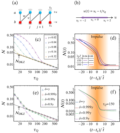
Figure 1: Dissipative quench dynamics of the Rice-Mele model. (a) The model in Eq. (11) in the presence of loss difference. (b) The quench protocol. (c) Fermion density left in the system after quench in the case of LLD ($\delta=\gamma$). The black solid line denotes the DKZ scaling behavior for long enough quench time. (d) Time evolution of fermion density in the case of LLD. The impulse stage near the critical point and the plateaus forming after the critical dynamics are shown. (e) and (f) Fermion density and its time evolution for several selected values of $\delta$ and $\gamma=0.08$. The dot-dashed lines in (c) and (e) are generated by the analytical formula in Eq. (15), perfectly matching the numerical solutions of the Lindblad equation indicated by the colored dingbats. In the calculation, we have set the parameters $v=-w=1$.

The DKZ scaling behavior is illustrated in Fig. 1(c). The stronger the loss dissipation on $a$ sublattice is, the shorter the quench time for the system to fall into the DKZ scaling behavior. Fig. 1(d) illustrate the time evolution of fermion density. Similar to the traditional KZ scaling law, the DKZ scaling law arises from the frozen effect near critical point, where the impulse stage is characterized by the frozen-out timescale $\hat{t}\sim\tau_{Q}^{z\nu/(1+z\nu)}$. On the other side, if we deviates from the LLD configuration, the result will acquire an exponentially decaying term, $e^{-\bar{u}(\gamma-\delta)\tau_{Q}}$, according to Eq. (15). For small deviation, the DKZ-like behavior can still be discerned somehow as shown in Fig. 1(e) and (f). While for large deviation ($\gamma\gg\delta$), the excitation density exponentially approaches the saturated value $\frac{1}{2}$ for strong dissipation and long quench time, because the system evolves into the pure steady state $|\psi(t_{f})\rangle=\bigotimes_{q}|0_{q}\rangle$ rapidly and nothing interesting is left.

It is noteworthy that the DKZ scaling law disclosed above can also be observed for the limit of gain difference. As can be seen if we replace the jump operators with $L_{a,j}=\sqrt{\gamma_{a}}c_{a,j}^{\dagger}$ and $L_{b,j}=\sqrt{\gamma_{b}}c_{b,j}^{\dagger}$. In this case, the system will gain lots of fermions and the scaling behaviors would be restated by the density of hole number instead.

V Shockley model: two types of scaling behaviors

Table 1: Protocols, LLD’s, and the consequent scaling behaviors of the fermion density for the Shockley model. There are two types of scaling behaviors, $\mathcal{N}_{\text{DKZ}}=\frac{1}{2\pi\sqrt{\tau_{Q}}}$ and $\mathcal{N}_{\text{D}}=\frac{A^{{}^{\prime}}}{(\gamma\tau_{Q})^{\alpha}}$. The quench protocols are represented by the colored arrows, where the on-site energy parameter is ramped from $u_{i}$ to $u_{f}$: $u_{i}=2v+1$ and $u_{f}=-(2v+1)$ for I, $u_{i}=0$ and $u_{f}=-(2v+1)$ for II, $u_{i}=2v+1$ and $u_{f}=0$ for III.

Shockley model
Quench protocol		LLD	$\mathcal{N}$	Figure
I		$\delta=\gamma$	$2\mathcal{N}_{\text{DKZ}}$	Fig. 2(a)
		$\delta=-\gamma$	-	-
II		$\delta=\gamma$	$\mathcal{N}_{\text{DKZ}}$	Fig. 2(b)
		$\delta=-\gamma$	$\mathcal{N}_{\text{D}}$	Fig. 2(c)
III		$\delta=\gamma$	$\mathcal{N}_{\text{DKZ}}+\mathcal{N}_{\text{D}}$	Fig. 2(d)
		$\delta=-\gamma$	-	-

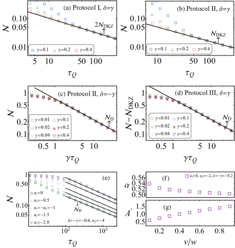
Figure 2: Dissipative quench dynamics of the Shockley model. (a)-(d) The fermion density left in the system after quench for the four cases that produce scaling behaviors, $\mathcal{N}_{\text{DKZ}}$ and/or $\mathcal{N}_{\text{D}}$, as listed in Table 1. (e) The fermion density for the case of protocol II and LLD, $\delta=-\gamma$, that produces $\mathcal{N}_{\text{D}}$. We have fixed the value of $\gamma=0.4$ and selected several values of $u_{i}$, which demonstrates that $\mathcal{N}_{\text{D}}$ is irrelevant to the critical dynamics since the system won’t be driven across the critical point for $u_{i}=-1.5$ and $-2.0$ at all. (f)-(g) The exponent $\alpha$ and prefactor $A^{{}^{\prime}}$ versus $v/w$ with fixed value of $w=1/2$. In (a)-(e), we have set $v=w=1/2$ and $\pm u_{c}=\pm 2v=\pm 1$.

The Shockley model reads [47]

$$H=\sum_{j}u\psi_{j}^{\dagger}\sigma_{z}\psi_{j}-\{\psi_{j}^{\dagger}(v\sigma_{z}+iw\sigma_{y})\psi_{j+1}+h.c.\},~{}$$ (17)

as depicted in the first line in Table. 1. Likewise, the Hamiltonian in the Fourier space can be reformulated as $H=\sum_{q}\textbf{d}(q)\cdot\sigma$, where $d^{x}_{q}=0,~{}d^{y}_{q}=2w\sin q,~{}d^{z}_{q}=u-2v\cos q$. Here, we ensure $w,v\geq 0$ and consider topological quantum phase transitions. The topologically trivial and nontrivial phases are distinguished by the winding number [48], $W=(1/2\pi)\int_{-\pi}^{\pi}(\tilde{\textbf{d}}\times\frac{\text{d}}{\text{d}q}\tilde{\textbf{d}})_{x}\text{d}q$ , where $\tilde{\textbf{d}}=\textbf{d}/|\textbf{d}|$. It takes the values $W=0$ for the trivial phase if $|u|>u_{c}$ and $W=1$ for the nontrivial phase if $|u|<u_{c}$. There are two critical points, $u=\pm u_{c}=\pm 2v$.

Besides the DKZ scaling behavior, we have found in the Shockley model that another type of scaling behavior irrelevant to the critical dynamics may also emerge in the LLD. We call it the dissipative scaling behavior that is expressed as

$$\mathcal{N}\approx\mathcal{N}_{\text{D}}=A^{{}^{\prime}}(\gamma\tau_{Q})^{-\alpha},$$ (18)

where the prefactor $A^{{}^{\prime}}$ and exponent $\alpha$ rely on the model parameters. With appropriate protocol, we may observe the two scaling behaviors, $\mathcal{N}_{\text{DKZ}}$ and $\mathcal{N}_{\text{D}}$, appear together or separately as listed in Table 1 and illustrated in Fig. 2.

Unlike the DKZ scaling behavior, the dissipative scaling behavior can be attributed to two factors having nothing to do with the critical dynamics. One is the presence of intra-sublattice hoppings, the other is the on-site energy parameter at the end of the quench, $u(t_{f})$, which favors the fermions to reside on the sublattices without dissipation. For example, let us see the case of protocol II with the LLD, $\delta=-\gamma$ or $\gamma_{b}>\gamma_{a}=0$, which produces the dissipative scaling behavior as illustrated in Fig. 2(c). In this case, there is no dissipation on the $a$ sublattice and the final value of the on-site energy parameter, $u(t_{f})=-2$, facilitates the fermions to reside on it, so that we have $\mathcal{N}\approx\mathcal{N}_{a}\approx\mathcal{N}_{\text{D}}$ and $\mathcal{N}_{b}\approx 0$.

VI Haldane model

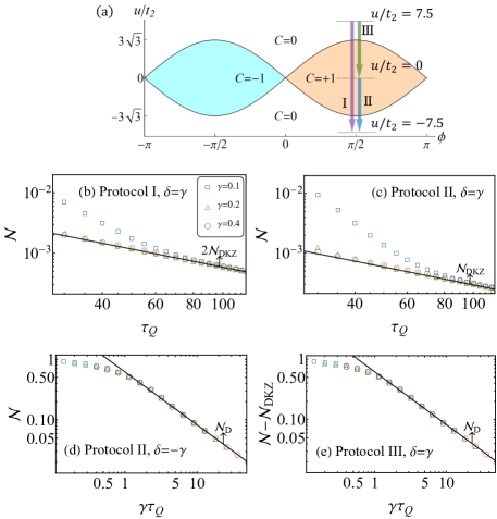
Figure 3: (a) Phase diagram of the Haldane model and the quench protocols I-III. (b)-(e) Density of fermion number for several values of $\gamma$. The calculation is performed on $150\times 150$ lattices with fixed parameters, $t_{1}=1$ and $t_{2}=1/3$. Here, the DKZ scaling reads $\mathcal{N}_{\text{DKZ}}=\frac{1}{2\sqrt{3}\pi^{2}\tau_{Q}}$, while the dissipative scaling reads $\mathcal{N}_{\text{D}}\sim(\gamma\tau_{Q})^{-\alpha}$.

The Haldane model is defined on a honeycomb lattices that can be decomposed into $a$ and $b$ sublattices [49, 50], on which two species of fermions reside respectively. So it allows us to apply the same scenario to explore the DKZ and dissipative scaling behaviors on it. The Hamiltonian is given by

$$H= -t_{1}\sum_{\langle i,j\rangle}\left(c_{i}^{\dagger}c_{j}+h.c.\right)-t_{2}\sum_{\langle\langle i,j\rangle\rangle}\left(e^{i\phi_{ij}}c_{i}^{\dagger}c_{j}+h.c.\right)$$

$$+u\sum_{i\in a}c_{i}^{\dagger}c_{i}-u\sum_{i\in b}c_{i}^{\dagger}c_{i},$$ (19)

where $t_{1}$ and $t_{2}$ is the nearest-neighbor and next-nearest-neighbor hopping term, $u$ is the on-site energy parameter, and $c_{i}^{(\dagger)}=c_{a(b),\textbf{r}}^{(\dagger)}$ is the creation (annihilation) operator on the sublattice $i\in a(b)$. $\phi_{ij}=\phi$ is the phase factor between the $a$ sublattice and $\phi_{ij}=-\phi$ between $b$ sublattice. The Chern number reads $C=\pm 1$ for $u/t_{2}<3\sqrt{3}|\sin\phi|$ and $C=0$ for other situations. By fixing the parameters, $t_{1}=1$ and $t_{2}=1/3$, we obtain the phase diagram illustrated in Fig. 3(a).

We shall omit the details of calculation and go straight to the results. The quench protocols I-III with the parameter $\phi=\pi/2$ are considered and depicted in the phase diagram. Like the situations listed in Table 1 for the Shockley model, we can also observe the DKZ scaling behavior $\mathcal{N}_{\text{DKZ}}$ and the scaling behavior $\mathcal{N}_{\text{D}}$ in the Haldane model as illustrated in Fig. 3(b)-(e).

VII Discussion

At last, we address two important issues. First, from the rigorous solutions in our situations, we have the benefit of diagnosing the interwinded roles of the non-Hermitian terms, $\frac{1}{2}\{\rho,L_{s,j}^{\dagger}L_{s,j}\}$, and the quantum jump terms, $L_{s,j}\rho L_{s,j}^{\dagger}$, in the Lindblad equation in Eq. (1). If we drop the quantum jump terms in Eq. (1), the system would be described by an effective non-Hermitian Hamiltonian [51], $H_{\text{eff}}=H-\frac{i}{2}\sum_{j}\sum_{s}L_{s,j}^{\dagger}L_{s,j}$. Qualitatively, this effective model can produce the DKZ behavior in the excitation density, but no AKZ behavior can be observed in it. The quantum jump terms are responsible for the AKZ behavior alone. More detailed analysis shows the quantum jump terms also give a correction to the prefactor of the DKZ scaling law to restore the full answer of the problem. While the fermion number $\mathcal{N}$ always contains no information of quantum jump, so we are not bothered by the AKZ behavior in measuring it.

Second, our conclusion is true for loss difference between the two sublattices of a bipartite lattice. Such kind of loss difference has been experimentally realized on the honeycomb photonic lattice [43], in which a non-Hermitian Hamiltonian similar to ours is discussed. In practice, the loss difference can also be realized for the two spin states, say $|\uparrow\rangle$ and $|\downarrow\rangle$, in the cold atom experiment [42]. A case in point is the Qi-Wu-Zhang model with two-band spectra [52, 48], in which we have confirmed the emergence of DKZ scaling behavior [46]. With these state-of-the-art experimental progresses, we expect the DKZ scaling law can be observed in near future.

VIII ACKNOWLEDGMENTS

We thank Jian-Song Pan, Yan He, and Uwe R. Fischer for insightful discussions. This work is supported by NSFC under Grant No. 11074177.

Supplemental Materials

S1. Two-Band Models in the Presence of Loss

A. Lindblad Master Equation

The two-band model on a bipartite lattice in momentum space reads

$$H=\sum_{q}\left(c_{a,q}^{\dagger}~{}c_{b,q}^{\dagger}\right)\left[d_{q}^{x}\sigma_{x}+d_{q}^{y}\sigma_{y}+d_{q}^{z}\sigma_{z}\right]\binom{c_{a,q}}{c_{b,q}},$$ (S18)

where $\sigma_{\mu}$’s represent a Pauli matrix, $c_{a,q}$ and $c_{b,q}$ denote the fermion operators on $a$ and $b$ sublattices respectively. By the canonical Bogoliubov transformation,

$$\eta_{1,q}=u_{q}c_{a,q}+v_{q}c_{b,q},~{}~{}\eta_{2,q}=-v_{q}^{*}c_{a,q}+u_{q}^{*}c_{b,q},$$ (S19)

with

$$\left(u_{q},v_{q}\right)=\left(\frac{\omega_{q}+d_{q}^{z}}{\sqrt{2\omega_{q}(\omega_{q}+d_{q}^{z})}},\frac{d_{q}^{x}-id_{q}^{y}}{\sqrt{2\omega_{q}(\omega_{q}+d_{q}^{z})}}\right),$$ (S20)

we obtain the diagonalized Hamiltonian,

$$H=\sum_{q}\omega_{q}(\eta_{1,q}^{\dagger}\eta_{1,q}-\eta_{2,q}^{\dagger}\eta_{2,q}),$$ (S21)

where the quasiparticle dispersion reads $\omega_{q}=\sqrt{|d_{q}^{x}|^{2}+|d_{q}^{y}|^{2}+|d_{q}^{z}|^{2}}$. We suppose a quantum phase transition occurs for a specific model at the gapless point of the dispersion, $\omega_{q_{c}}=0$, with the critical mode $q_{c}$.

We introduce a linear ramp in the Hamiltonian in Eq. (S18),

$$d_{q}^{z}~{}\rightarrow~{}d_{q}^{z}(t)=d_{q}^{z}(t_{i})-\frac{t}{\tau_{Q}},~{}(t_{i}\leq t\leq t_{f})$$ (S22)

where $\tau_{Q}$ is the quench time, $t_{i}=0$, $t_{f}\gg 0$, $d_{q}^{z}(t_{i})\gg 0$, and $d_{q}^{z}(t_{f})\ll 0$. We can rewrite the time-dependent Hamiltonian by a $4\times 4$ matrix,

$$H(t)=\sum_{q}\phi_{q}^{\dagger}\left(\begin{array}[]{cccc}0&0&0&0\\ 0&d_{q}^{z}(t_{i})-t/\tau_{Q}&d^{x}_{q}-id^{y}_{q}&0\\ 0&d^{x}_{q}+id^{y}_{q}&-d_{q}^{z}(t_{i})+t/\tau_{Q}&0\\ 0&0&0&0\end{array}\right)\phi_{q}$$ (S23)

in the basis vector $\phi_{q}^{\dagger}=(|0\rangle,c_{a,q}^{\dagger}|0\rangle,c_{b,q}^{\dagger}|0\rangle,c_{a,q}^{\dagger}c_{b,q}^{\dagger}|0\rangle)$. The density matrix $\rho(t)$ can be expressed in the Fourier space as $\rho(t)=\bigotimes_{q}\rho_{q}(t)$, where

$$\rho_{q}=\left(\begin{array}[]{cccc}\rho_{q}^{(11)}&0&0&0\\ 0&\rho_{q}^{(22)}&\rho_{q}^{(23)}&0\\ 0&\rho_{q}^{(32)}&\rho_{q}^{(33)}&0\\ 0&0&0&\rho_{q}^{(44)}\end{array}\right).$$ (S24)

The matrix representations of the operators are given by

$$c_{a,q}=\left(\begin{array}[]{cccc}0&1&0&0\\ 0&0&0&0\\ 0&0&0&1\\ 0&0&0&0\end{array}\right),~{}c_{b,q}=\left(\begin{array}[]{cccc}0&0&1&0\\ 0&0&0&-1\\ 0&0&0&0\\ 0&0&0&0\end{array}\right),~{}\eta_{1,q}=\left(\begin{array}[]{cccc}0&u_{q}&v_{q}&0\\ 0&0&0&v_{q}\\ 0&0&0&u_{q}\\ 0&0&0&0\end{array}\right),~{}\eta_{2,q}=\left(\begin{array}[]{cccc}0&-v_{q}^{*}&u_{q}^{*}&0\\ 0&0&0&-u_{q}^{*}\\ 0&0&0&-v_{q}^{*}\\ 0&0&0&0\end{array}\right).$$ (S25)

When the system interacts with the environment, the dynamics of the system can be described by the Lindblad master equation [26, 28, 53],

$$\frac{\partial}{\partial t}\rho=-i[H(t),\rho]+\sum_{q}\mathcal{D}_{q}[\rho_{q}],$$ (S26)

where the term of loss is given by

$$\mathcal{D}_{q}[\rho_{q}]= \gamma_{a}\left(c_{a,q}\rho_{q}c_{a,q}^{\dagger}-\frac{1}{2}\{\rho_{q},c_{a,q}^{\dagger}c_{a,q}\}\right)+\gamma_{b}\left(c_{b,q}\rho_{q}c_{b,q}^{\dagger}-\frac{1}{2}\{\rho_{q},c_{b,q}^{\dagger}c_{b,q}\}\right).$$ (S27)

By Eqs. (S23), (S24) and (S25), we get a set of first-order differential equations,

$$\frac{d\rho_{q}^{(11)}}{dt} =\gamma_{a}\rho_{q}^{(22)}+\gamma_{b}\rho_{q}^{(33)},$$ (S28a)

$$\frac{d\rho_{q}^{(22)}}{dt} =-\gamma_{a}\rho_{q}^{(22)}+\gamma_{b}\rho_{q}^{(44)}+i\Delta_{q}\rho_{q}^{(23)}-i\Delta_{q}^{*}\rho_{q}^{(32)},$$ (S28b)

$$\frac{d\rho_{q}^{(33)}}{dt} =-\gamma_{b}\rho_{q}^{(33)}+\gamma_{a}\rho_{q}^{(44)}-i\Delta_{q}\rho_{q}^{(23)}+i\Delta_{q}^{*}\rho_{q}^{(32)},$$ (S28c)

$$\frac{d\rho_{q}^{(44)}}{dt} =-\gamma_{a}\rho_{q}^{(44)}-\gamma_{b}\rho_{q}^{(44)},$$ (S28d)

$$\frac{d\rho_{q}^{(23)}}{dt} =-\frac{1}{2}(\gamma_{a}+\gamma_{b})\rho_{q}^{(23)}-2id_{q}^{z}(t)\rho_{q}^{(23)}+i\Delta_{q}^{*}(\rho_{q}^{(22)}-\rho_{q}^{(33)}),$$ (S28e)

$$\frac{d\rho_{q}^{(32)}}{dt} =-\frac{1}{2}(\gamma_{a}+\gamma_{b})\rho_{q}^{(32)}+2id_{q}^{z}(t)\rho_{q}^{(32)}-i\Delta_{q}(\rho_{q}^{(22)}-\rho_{q}^{(33)}),$$ (S28f)

where $\Delta_{q}=d^{x}_{q}+id^{y}_{q}$. The initial conditions at $t=t_{i}=0$ read

$$\rho_{q}^{(33)}=1,~{}~{}\rho_{q}^{(11)}=\rho_{q}^{(22)}=\rho_{q}^{(44)}=0,~{}~{}\rho_{q}^{(23)}=(\rho_{q}^{(32)})^{*}=0$$ (S29)

for $d_{q}^{z}(t_{i})\gg 1$.

By defining

$$R_{q}=\rho_{q}^{(33)}-\rho_{q}^{(22)}=e^{-\frac{1}{2}\gamma t}\tilde{R}_{q},~{}~{}R_{q}^{\prime}=\rho_{q}^{(11)}-\rho_{q}^{(44)}=e^{-\frac{1}{2}\gamma t}\tilde{R}_{q}^{\prime},~{}~{}\rho_{q}^{(23)}=e^{-\frac{1}{2}\gamma t}\tilde{\rho}_{q}^{(23)},$$ (S30)

we can transform the equations in Eq. (S28) into a set of integral-differential equations

$$\tilde{R}_{q}^{\prime}= (e^{\gamma t/2}-1)-\frac{\gamma_{a}-\gamma_{b}}{2}\int_{0}^{t}dt^{\prime}\tilde{R}_{q}(t^{\prime}),$$ (S31a)

$$\tilde{\rho}_{q}^{(23)}= (\tilde{\rho}_{q}^{(32)})^{*}=-i\Delta_{q}\int_{0}^{t}\tilde{R}_{q}(t^{\prime})e^{\left(2i\int_{0}^{t}d_{q}^{z}(t^{\prime})dt^{\prime}-2\int_{0}^{t^{\prime}}d_{q}^{z}(t^{\prime\prime})dt^{\prime\prime}\right)}dt^{\prime},$$ (S31b)

$$\frac{d\tilde{R}_{q}(t)}{dt}= \frac{\gamma_{a}-\gamma_{b}}{2}+\frac{(\gamma_{a}-\gamma_{b})^{2}}{4}\int_{0}^{t}dt^{\prime}\tilde{R}_{q}(t^{\prime})-4|\Delta_{q}|^{2}\int_{0}^{t}\tilde{R}_{q}(t^{\prime})\cos\left(2\int_{0}^{t}d_{q}^{z}(t^{\prime})dt^{\prime}-2\int_{0}^{t^{\prime}}d_{q}^{z}(t^{\prime\prime})dt^{\prime\prime}\right)dt^{\prime}.$$ (S31c)

B. Exact Solution in the Absence of Loss, $\gamma_{a}=\gamma_{b}=0$

Now, we revisit the conventional Kibbke-Zurek mechanism (KZM) by the Lindblad formalism for $\forall\gamma_{i}=0$. Eq. (S31c) becomes

$$\frac{dR_{q}(s)}{ds} =-4|\Delta_{q}|^{2}\tau_{Q}\int_{s_{i}}^{s}R_{q}(s^{\prime})\cos\left(s^{2}-s^{\prime 2}\right)ds^{\prime}$$ (S32)

where $s=[t-d_{q}^{z}(t_{i})\tau_{Q}]/\sqrt{\tau_{Q}}$, $s_{i}=-\sqrt{\tau_{Q}}d_{q}^{z}(t_{i})$, and the initial condition $R_{q}(0)=1$.

According to KZM, only the modes near $q_{c}$ can be significantly excited ($|q-q_{c}|\sim 0$). For modes far away from $q_{c}$, we get the solution of Eq. (S32),

$$R_{q}=2|u_{q}|^{2}-1~{}~{}~{}(|q-q_{c}|\gg 0).$$ (S33)

While in the vicinity of $q_{c}$ and in the absence of dissipation, the integral-differential equation can be solved iteratively as [44, 45],

$$R_{q}=1+\sum_{j=1}^{\infty}(-4|\Delta_{q}|^{2}\tau_{Q})^{j}\left[\prod_{l=0}^{j}\int_{s_{i}}^{s_{2l-1}}ds_{2l}\int_{s_{i}}^{s_{2l}}ds_{2l+1}\cos(s_{2l}^{2}-s_{2l+1}^{2})\right].$$ (S34)

For slow ramp (i.e. $\tau_{Q}$ is large enough), we can set $s_{i}\rightarrow-\infty$, which leads to the long-time asymptotic solution exactly,

$$R_{q}=1+\sum_{j=1}^{\infty}(-4|\Delta_{q}|^{2}\tau_{Q})^{j}\frac{\pi^{j}}{2^{2j-1}j!}=2e^{-\pi\tau_{Q}|\Delta_{q}|^{2}}-1,~{}~{}~{}(|q-q_{c}|\sim 0).$$ (S35)

Usually we assume the linear behavior, $|\Delta_{q}|\propto|q-q_{c}|$ in Eq. (S35). Combining Eqs. (S33) and (S35), we obtain the solution for $R_{q}$ after quench

$$R_{q}=2e^{-\pi\tau_{Q}|\Delta_{q}|^{2}}+2|u_{q}|^{2}-1.$$ (S36)

Near $q_{c}$, we have $(u_{q},v_{q})=(0,1)$ since $d_{q}^{x}\sim 0$, $d_{q}^{y}\sim 0$, $d_{q}^{z}(t_{f})\ll 0$ and

$$\left|\frac{u_{q}}{v_{q}}\right|=\frac{|d_{q}^{z}(t_{f})|\sqrt{1+[(d_{q}^{x})^{2}+(d_{q}^{y})^{2}]/(d_{q}^{z})^{2}}-|d_{q}^{z}(t_{f})|}{\sqrt{(d_{q}^{x})^{2}+(d_{q}^{y})^{2}}}\approx\frac{\sqrt{(d_{q}^{x})^{2}+(d_{q}^{y})^{2}}}{2|d_{q}^{z}(t_{f})|}\approx 0.$$ (S37)

Thus Eq. (S35) is recovered when $q\rightarrow q_{c}$. Away from $q_{c}$, we have $e^{-\pi\tau_{Q}|\Delta_{q}|^{2}}=0$, so that Eq. (S33) is recovered.

By $\rho_{q}^{(22)}+\rho_{q}^{(33)}=1$ and $\rho_{q}^{(33)}-\rho_{q}^{(22)}=R_{q}$, we get

$$\rho_{q}^{(22)}= (1-R_{q})/2=1-|u_{q}|^{2}-e^{-\pi\tau_{Q}|\Delta_{q}|^{2}}$$ (S38)

$$\rho_{q}^{(33)}= (1+R_{q})/2=|u_{q}|^{2}+e^{-\pi\tau_{Q}|\Delta_{q}|^{2}},$$ (S39)

and

$$\rho_{q}^{(23)}=(\rho_{q}^{(32)})^{*}=-\sqrt{e^{-\pi\tau_{Q}|\Delta_{q}|^{2}}(1-e^{-\pi\tau_{Q}|\Delta_{q}|^{2}})}e^{i\theta_{q}}-u_{q}^{*}v_{q},$$ (S40)

where $\theta_{q}$ is the dynamical phase [9].

C. Exact Solution in the Presence of Uniform Loss, $\gamma_{a}=\gamma_{b}\neq 0$

For the situation of uniform loss, $\gamma_{a}=\gamma_{b}\neq 0$, the equation in Eq. (S31c) can be simplified to

$$\frac{d\tilde{R}_{q}(s)}{ds} =-4|\Delta_{q}|^{2}\tau_{Q}\int_{s_{i}}^{s}\tilde{R}_{q}(s^{\prime})\cos\left(s^{2}-s^{\prime 2}\right)ds^{\prime},$$ (S41)

where $s=[t-d_{q}^{z}(t_{i})\tau_{Q}]/\sqrt{\tau_{Q}}$ and $s_{i}=-d_{q}^{z}(t_{i})\sqrt{\tau_{Q}}$, which has the same form as that in Eq. (S32) and shares the same initial condition, $\tilde{R}_{q}(0)=R_{q}(0)=1$. The full solution of $\tilde{R}_{q}(t)$ is expressed by the Fresnel’s integrals in Eq. (S34). However, we only need to concern the solution at the final time ($t=t_{f}$), which can be exactly worked out by asymptotic analysis [44, 45],

$$\tilde{R}_{q}(t_{f})=e^{\bar{u}\gamma\tau_{Q}}\left(\rho_{q}^{(33)}-\rho_{q}^{(22)}\right)=2e^{-\pi\tau_{Q}|\Delta_{q}|^{2}}+2|u_{q}|^{2}-1,$$ (S42)

in which we have defined $\bar{u}=[d_{q}^{z}(t_{i})-d_{q}^{z}(t_{f})]/2$. Moveover, the solution of Eq. (S31a) is given by

$$\tilde{R}_{q}^{\prime}(t)=e^{\gamma t/2}\left(\rho_{q}^{(11)}-\rho_{q}^{(44)}\right)=e^{\gamma t/2}-1.$$ (S43)

And by Eq. (S28d), we have

$$\rho_{q}^{(44)}=0.$$ (S44)

So, the solution of the set of equations in Eq. (S28) is given by

$$\rho_{q}^{(11)}=1-e^{-\bar{u}\gamma\tau_{Q}},$$ (S45a)

$$\rho_{q}^{(22)}=\frac{1}{2}-\frac{1}{2}e^{-\bar{u}\gamma\tau_{Q}}\tilde{R}_{q}-\frac{1}{2}(1-e^{-\bar{u}\gamma\tau_{Q}})=e^{-\bar{u}\gamma\tau_{Q}}\left(|v_{q}|^{2}-e^{-\pi\tau_{Q}|\Delta_{q}|^{2}}\right),$$ (S45b)

$$\rho_{q}^{(33)}=\frac{1}{2}+\frac{1}{2}e^{-\bar{u}\gamma\tau_{Q}}\tilde{R}_{q}-\frac{1}{2}(1-e^{-\bar{u}\gamma\tau_{Q}})=e^{-\bar{u}\gamma\tau_{Q}}\left(|u_{q}|^{2}+e^{-\pi\tau_{Q}|\Delta_{q}|^{2}}\right),$$ (S45c)

$$\rho_{q}^{(44)}=0,$$ (S45d)

$$\rho_{q}^{(23)}=(\rho_{q}^{(32)})^{*}=-e^{-\bar{u}\gamma\tau_{Q}}\left[\sqrt{e^{-\pi\tau_{Q}|\Delta_{q}|^{2}}(1-e^{-\pi\tau_{Q}|\Delta_{q}|^{2}})}e^{i\theta_{q}}+u_{q}^{*}v_{q}\right],$$ (S45e)

at the final time $t_{f}$ of the quench.

S2. Dissipative Critical Dynamics of the Rice-Mele Model

A. The model Hamiltonian

The Rice-Mele model (RRM) is given by

$$H= \sum_{j=1}^{N}\left(vc_{a,j}^{\dagger}c_{b,j}-wc_{a,j+1}^{\dagger}c_{b,j}+h.c.\right)+u\sum_{j=1}^{N}\left(c_{a,j}^{\dagger}c_{a,j}-c_{b,j}^{\dagger}c_{b,j}\right).$$ (S46)

By the Fourier transformation $c_{a(b),q}=\sum_{j}\frac{e^{-iqj}}{\sqrt{N}}c_{a(b),j}$, the Hamiltonian here can be expressed in the form like the one in Eq. (S18) with

$$\textbf{d}(q)=(d^{x}_{q},d^{y}_{q},d^{z}_{q})=(v+w\cos q,w\sin q,u).$$ (S47)

The quasiparticle dispersion is worked out as $\omega_{q}=|\textbf{d}(q)|=\sqrt{u^{2}+w^{2}\sin^{2}q+(v+w\cos q)^{2}}$. The system exhibits two critical points: one at $v=w$ and $u=u_{c}=0$ with a critical momentum $q_{c}=\pi$, and the other at $v=-w$ and $u=u_{c}=0$ with a critical momentum $q_{c}=0$. For convenience, we set the reference energy scale such that

$$v=-w=1.$$ (S48)

The linear ramp reads,

$$u=u(t)=u_{i}-\frac{t}{\tau_{Q}}~{}~{}~{}(0\leq t\leq t_{f}).$$ (S49)

The on-site energy parameter is linearly ramped across the quantum phase transition point $u_{c}$ satisfying $u_{i}\geq u_{c}\geq u_{f}=u(t_{f})$. The resulting Lindblad equation falls into the general form in Eqs. (S26) and (S27).

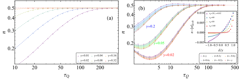
Figure S4: Density of excitations in the Rice-Mele model for the case of uniform loss, $\gamma_{a}=\gamma_{b}$, in panel (a) and the case of loss difference, $\gamma_{a}\neq\gamma_{b}$, in panel (b). We select parameters $h_{i}=2$ and $h_{f}=-2$. In panel (a), the numerical results obtained from the Lindblad equation in Eq. (S28) are represented by the colored dingbats. They match the analytical solution in Eq. (S51) represented by dash-dotted lines perfectly. In panel (b), the numerical results, also represented by the colored dingbats, match the analytical solution in Eq. (S60) represented by the dash-dotted lines perfectly. The inset in panel (b) illustrates how the excitation densities vary with the variable $\delta$.

B. Exact Solution in the Presence of Uniform Loss, $\gamma_{a}=\gamma_{b}\neq 0$

Due to the solution of Eq. (S45), the excitation probability for the case of uniform loss, $\gamma_{a}=\gamma_{b}$, reads

$$p_{q} =\frac{1}{2}\text{Tr}(\rho_{q}\eta_{1,q}^{\dagger}\eta_{1,q})+\frac{1}{2}\text{Tr}[\rho_{q}(1-\eta_{2,q}^{\dagger}\eta_{2,q})]$$

$$=|v_{q}|^{2}\rho_{q}^{(33)}+|u_{q}|^{2}\rho_{q}^{(22)}+\frac{1}{2}\left(\rho_{q}^{(11)}+\rho_{q}^{(44)}\right)+\left(u_{q}v_{q}^{*}\rho_{q}^{(23)}+u_{q}^{*}v_{q}\rho_{q}^{(32)}\right)$$

$$\approx e^{-\bar{u}\gamma\tau_{Q}}e^{-\pi\tau_{Q}q^{2}}+\frac{1}{2}(1-e^{-\bar{u}\gamma\tau_{Q}})$$ (S50)

where $|\Delta_{q}|^{2}=q^{2}$ and $\bar{u}=(u_{i}-u_{f})/2$, and the density of the excitation probability is given by

$$n =\frac{1}{N}\sum_{q}p_{q}=\int_{0}^{\pi}\frac{dq}{2\pi}p_{q}=\frac{1}{2}\left(1-e^{-\bar{u}\gamma\tau_{Q}}\right)+\frac{e^{-\bar{u}\gamma\tau_{Q}}}{2\pi\sqrt{\tau_{Q}}},$$ (S51)

where the numerical evidence is depicted in Fig. S4(a). The fermion numbers at sublattice $a$ and $b$ are expressed as

$$\mathcal{N}_{a}= \frac{1}{N}\sum_{q}\text{Tr}(\rho c_{a,q}^{\dagger}c_{a,q})=e^{-\bar{u}\gamma\tau_{Q}}\left(\mathcal{N}_{a}^{\text{GS}}-\frac{1}{2\pi\sqrt{\tau_{Q}}}\right)$$ (S52)

$$\mathcal{N}_{b}= \frac{1}{N}\sum_{q}\text{Tr}(\rho c_{b,q}^{\dagger}c_{b,q})=e^{-\bar{u}\gamma\tau_{Q}}\left(\mathcal{N}_{b}^{\text{GS}}+\frac{1}{2\pi\sqrt{\tau_{Q}}}\right).$$ (S53)

C. Rigorous Solution in the Presence of Loss Difference, $\gamma_{a}\neq\gamma_{b}$

We now discuss the loss difference, i.e. $\delta\equiv\gamma_{a}-\gamma_{b}\neq 0$. The equations in Eqs. (S31a) and (S31c) become

$$\frac{d\tilde{R}_{q}^{\prime}(t)}{dt} = e^{\gamma t/2}-1-\frac{\delta}{2}\int_{0}^{t}dt^{\prime}\tilde{R}_{q}(t^{\prime}),$$ (S54a)

$$\frac{d\tilde{R}_{q}(t)}{dt} = \frac{\delta}{2}+\left(\frac{\delta}{2}\right)^{2}\int_{0}^{t}dt^{\prime}\tilde{R}_{q}(t^{\prime})-4|\Delta_{q}|^{2}\int_{x_{i}}^{x}\tilde{R}_{q}(x^{\prime})\cos\left[\frac{x^{2}-(x^{\prime})^{2}}{\tau_{Q}}\right]dx^{\prime},$$ (S54b)

where $x=t-u_{i}\tau_{Q}$ and $x_{i}=-u_{i}\tau_{Q}$. The initial conditions read $\tilde{R}_{q}(0)=1$ and $\tilde{R}^{\prime}_{q}(0)=0$. We speculate the solution in two steps. First, let us consider the solution for $q=0$, which means $\Delta_{q}=0$ so that the last term in Eq. (S54b) disappears and the solution is given by

$$\tilde{R}_{0}(t)=e^{\delta t/2},~{}~{}~{}~{}\tilde{R}^{\prime}_{0}(t)=e^{\gamma t/2}+e^{\delta t/2}-2.$$ (S55)

Next, we consider $q\neq 0$ and speculate the solution of $\tilde{R}_{q}(t)$ as,

$$\tilde{R}_{q}(t)=\left[\tilde{R}_{q}(t)\right]_{\delta=0}+g(q,t)(e^{\delta t/2}-1),~{}~{}\tilde{R}^{\prime}_{q}(t)=\left[\tilde{R}^{\prime}_{q}(t)\right]_{\delta=0}+h(q,t)(e^{\delta t/2}-1),$$ (S56)

where $g(0,t)=h(0,t)=1$. For arbitrary time $t$, $\left[\tilde{R}^{\prime}_{q}(t)\right]_{\delta=0}$ is just the solution in Eq. (S43). While $\left[\tilde{R}_{q}(t)\right]_{\delta=0}$ should resort to the iterative method like that in Eq. (S34), but again we can only concern the final time of the quench and work out the asymptotic result as ($t_{f}=2\bar{u}\tau_{Q}$ here)

$$\tilde{R}_{q}=\tilde{R}_{q}(t_{f}) = 2e^{-\pi\tau_{Q}q^{2}}+2|u_{q}|^{2}-1+e^{-\pi\tau_{Q}q^{2}}(e^{\bar{u}\delta\tau_{Q}}-1),$$ (S57a)

$$\tilde{R}_{q}^{\prime}=\tilde{R}_{q}^{\prime}(t_{f}) = e^{\bar{u}\gamma\tau_{Q}}-1-e^{-\pi\tau_{Q}q^{2}}\left(e^{\bar{u}\delta\tau_{Q}}-1\right).$$ (S57b)

In order to verify these analytical expressions, we have defined two functions according to Eq. (S56),

$$g(q,t_{f})=\frac{\tilde{R}_{q}(t_{f})-\left[\tilde{R}_{q}(t_{f})\right]_{\delta=0}}{e^{\delta t_{f}/2}-1},~{}~{}~{}h(q,t_{f})=\frac{\tilde{R}^{\prime}_{q}(t_{f})-\left[\tilde{R}^{\prime}_{q}(t_{f})\right]_{\delta=0}}{e^{\delta t_{f}/2}-1},$$ (S58)

and compare them with the numerical results by solving the equations in Eq. (S28). As shown in Fig. S5, we see the analytical solution in Eq. (S57) is quite satisfactory. Thus, we can list all solutions for the case of $\gamma_{a}\neq\gamma_{b}$ as below,

$$R_{q}= e^{-\bar{u}\gamma\tau_{Q}}(2e^{-\pi\tau_{Q}q^{2}}+2|u_{q}|^{2}-1)+e^{-\pi\tau_{Q}q^{2}}\frac{e^{\bar{u}\delta\tau_{Q}}-1}{e^{\bar{u}\gamma\tau_{Q}}},$$ (S59a)

$$R_{q}^{\prime}= 1-e^{-\bar{u}\gamma\tau_{Q}}-e^{-\pi\tau_{Q}q^{2}}\frac{e^{\bar{u}\delta\tau_{Q}}-1}{e^{\bar{u}\gamma\tau_{Q}}},$$ (S59b)

$$\rho^{(11)}_{q}= 1-e^{-\bar{u}\gamma\tau_{Q}}-e^{-\pi\tau_{Q}q^{2}}\frac{e^{\bar{u}\delta\tau_{Q}}-1}{e^{\bar{u}\gamma\tau_{Q}}},$$ (S59c)

$$\rho^{(22)}_{q}= e^{-\bar{u}\gamma\tau_{Q}}\left(1-|u_{q}|^{2}-e^{-\pi\tau_{Q}q^{2}}\right),$$ (S59d)

$$\rho^{(33)}_{q}= e^{-\bar{u}\gamma\tau_{Q}}\left(|u_{q}|^{2}+e^{-\pi\tau_{Q}q^{2}}\right)+e^{-\pi\tau_{Q}q^{2}}\frac{e^{\bar{u}\delta\tau_{Q}}-1}{e^{\bar{u}\gamma\tau_{Q}}},$$ (S59e)

$$\rho^{(44)}_{q}= 0.$$ (S59f)

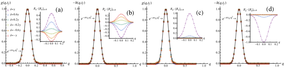
Figure S5: The functions $g(q,t_{f})$ and $h(q,t_{f})$ versus $q$ in the Rice-Mele model in the presence of loss difference. We have fixed the parameters, $u_{i}=2$, $u_{f}=-2$, $\tau_{Q}=30$, and $\gamma_{a}+\gamma_{b}=0.01$ for panels (a) and (b), while $\gamma_{a}+\gamma_{b}=0.1$ for panels (c) and (d). The numerical results indicated by the colored dingbats are obtained from solving the equations in Eq. (S28). The analytical functions are denoted by the black lines. In the insets of panels (a) and (c), the dash-dotted lines represent the solution in Eq. (S59a). While in the insets of panels (b) and (d), the dash-dotted lines represent the solution in Eq. (S59b). We see the analytical expressions match the numerical results rigorously.

The density of excitations is worked out as

$$n=\frac{e^{-\bar{u}\gamma\tau_{Q}}}{2\pi\sqrt{\tau_{Q}}}+\frac{1}{2}(1-e^{-\bar{u}\gamma\tau_{Q}})+\frac{e^{\bar{u}\delta\tau_{Q}}-1}{e^{\bar{u}\gamma\tau_{Q}}}\frac{1}{4\pi\sqrt{\tau_{Q}}},$$ (S60)

whose numerical results are depicted in Fig. S4(b). In Eq. (S60), the first term comes from $\rho_{q}^{(22)}$ and $\rho_{q}^{(33)}$ that is generated by the non-Hermitian terms of the Lindblad equation, the second term is attributed to $\rho_{q}^{(11)}$ that is generated by the quantum jump terms, and the third term comes from $\rho_{q}^{(11)}$ and $\rho_{q}^{(33)}$. In the limit of loss difference (LLD), i.e. $\gamma=\delta$, a universal DKZ scaling law emerge as $n-1/2\approx n_{\text{DKZ}}=\frac{1}{4\pi\sqrt{\tau_{Q}}}$ for large enough $\tau_{Q}$, in which $\rho_{q}^{(33)}$ produces $2n_{\text{DKZ}}$ while $\rho_{q}^{(11)}$ generates $-n_{\text{DKZ}}$.

The fermion numbers on sublattice $a$ and $b$ are worked out as

$$\mathcal{N}_{a}= e^{-\bar{u}\gamma\tau_{Q}}\left(\mathcal{N}_{a}^{\text{GS}}-\frac{1}{2\pi\sqrt{\tau_{Q}}}\right)$$ (S61a)

$$\mathcal{N}_{b}= e^{-\bar{u}\gamma\tau_{Q}}\left(\mathcal{N}_{b}^{\text{GS}}+\frac{1}{2\pi\sqrt{\tau_{Q}}}\right)+\frac{e^{\bar{u}\delta\tau_{Q}}-1}{e^{\bar{u}\gamma\tau_{Q}}}\frac{1}{2\pi\sqrt{\tau_{Q}}}.$$ (S61b)

respectively. The numerical results are depicted in Fig. S6, which rigorously fits the analytical expressions in Eq. (S61). Finally, we summarize the above results in Table S2.

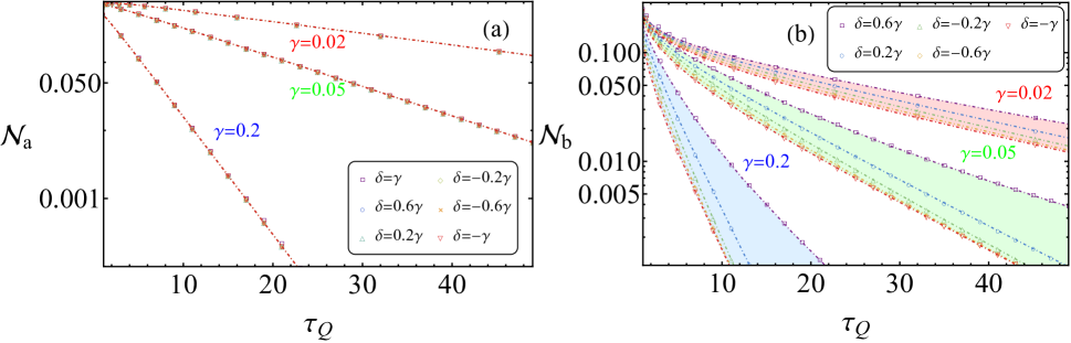
Figure S6: Fermion density in the Rice-Mele model in the presence of loss difference. We have set the parameters, $u_{i}=2$ and $u_{f}=-2$. The numerical results represented by the color dingbats are obtained by solving the Lindblad equation in Eq. (S28). The dash-dotted lines in panels (a) and (b) correspond to the analytical solutions in Eqs. (S61a) and (S61b) respectively.

Table S2: Excitation and fermion densities in the Rice-Mele model for $\gamma_{a}=\gamma_{b}=0$, $\gamma_{a}=\gamma_{b}\neq 0$, and $\gamma_{a}\neq\gamma_{b}$.

	$\gamma_{a}=\gamma_{b}=0$	$\gamma_{a}=\gamma_{b}\neq 0$	$\gamma_{a}\neq\gamma_{b}~{}~{}(\delta=\gamma_{a}-\gamma_{b}\neq 0)$
Excitation density $n=\frac{1}{N}\sum_{q}p_{q}$	$\frac{1}{2\pi\sqrt{\tau_{Q}}}$	$\frac{e^{-\bar{u}\gamma\tau_{Q}}}{2\pi\sqrt{\tau_{Q}}}+\frac{1}{2}(1-e^{-\bar{u}\gamma\tau_{Q}})$	$\frac{e^{-\bar{u}\gamma\tau_{Q}}}{2\pi\sqrt{\tau_{Q}}}+\frac{1}{2}(1-e^{-\bar{u}\gamma\tau_{Q}})+\frac{e^{\bar{u}\delta\tau_{Q}}-1}{e^{\bar{u}\gamma\tau_{Q}}}\frac{1}{4\pi\sqrt{\tau_{Q}}}$
Fermion number at $A$ $\mathcal{N}_{a}=\frac{1}{N}\sum_{q}\text{Tr}(\rho c_{a,q}^{\dagger}c_{a,q})$	$\mathcal{N}_{a}^{\text{GS}}-\frac{1}{2\pi\sqrt{\tau_{Q}}}$	$e^{-\bar{u}\gamma\tau_{Q}}\left(\mathcal{N}_{a}^{\text{GS}}-\frac{1}{2\pi\sqrt{\tau_{Q}}}\right)$	$e^{-\bar{u}\gamma\tau_{Q}}\left(\mathcal{N}_{a}^{\text{GS}}-\frac{1}{2\pi\sqrt{\tau_{Q}}}\right)$
Fermion number at $B$ $\mathcal{N}_{b}=\frac{1}{N}\sum_{q}\text{Tr}(\rho c_{b,q}^{\dagger}c_{b,q})$	$\mathcal{N}_{b}^{\text{GS}}+\frac{1}{2\pi\sqrt{\tau_{Q}}}$	$e^{-\bar{u}\gamma\tau_{Q}}\left(\mathcal{N}_{b}^{\text{GS}}+\frac{1}{2\pi\sqrt{\tau_{Q}}}\right)$	$e^{-\bar{u}\gamma\tau_{Q}}\left(\mathcal{N}_{b}^{\text{GS}}+\frac{1}{2\pi\sqrt{\tau_{Q}}}\right)+\frac{e^{\bar{u}\delta\tau_{Q}}-1}{e^{\bar{u}\gamma\tau_{Q}}}\frac{1}{2\pi\sqrt{\tau_{Q}}}$

S3. Effective Non-Hermitian System with Loss Difference for the Rice-Mele Model

By ignoring the quantum jump terms in Eq. (S26), we get

$$\frac{\partial}{\partial t}\rho=-i[H(t),\rho]-\frac{1}{2}\sum_{q}(\gamma_{a}\{\rho_{q},c_{a,q}^{\dagger}c_{a,q}\}+\gamma_{b}\{\rho_{q},c_{b,q}^{\dagger}c_{b,q}\}).$$ (S62)

Or explicitly, we have

$$\frac{d\rho_{q}^{(22)}}{dt} =-\gamma_{a}\frac{\rho_{q}^{(33)}+\rho_{q}^{(22)}}{2}+\gamma_{a}\frac{\rho_{q}^{(33)}-\rho_{q}^{(22)}}{2}+i\Delta_{q}\rho_{q}^{(23)}-i\Delta_{q}^{*}\rho_{q}^{(32)},$$ (S63a)

$$\frac{d\rho_{q}^{(33)}}{dt} =-\gamma_{b}\frac{\rho_{q}^{(33)}+\rho_{q}^{(22)}}{2}-\gamma_{b}\frac{\rho_{q}^{(33)}-\rho_{q}^{(22)}}{2}-i\Delta_{q}\rho_{q}^{(23)}+i\Delta_{q}^{*}\rho_{q}^{(32)},$$ (S63b)

$$\frac{d\rho_{q}^{(23)}}{dt} =-\frac{1}{2}(\gamma_{a}+\gamma_{b})\rho_{q}^{(23)}-2iu(t)\rho_{q}^{(23)}+i\Delta_{q}^{*}(\rho_{q}^{(22)}-\rho_{q}^{(33)}),$$ (S63c)

$$\frac{d\rho_{q}^{(32)}}{dt} =-\frac{1}{2}(\gamma_{a}+\gamma_{b})\rho_{q}^{(32)}+2iu(t)\rho_{q}^{(32)}-i\Delta_{q}(\rho_{q}^{(22)}-\rho_{q}^{(33)}).$$ (S63d)

And subsequently, we get

$$\tilde{\mathcal{R}}_{q}=1+\frac{\delta}{2}\int_{0}^{t}\tilde{R}_{q}dt^{\prime},$$ (S64a)

$$\frac{d\tilde{R}_{q}}{dt}=\frac{\delta}{2}+\left(\frac{\delta}{2}\right)^{2}\int_{0}^{t}\tilde{R}_{q}dt^{\prime}-4|\Delta_{q}|^{2}\int_{x_{i}}^{x}\tilde{R}_{q}(x^{\prime})\cos\left[\frac{x^{2}-(x^{\prime})^{2}}{\tau_{Q}}\right]dx^{\prime},$$ (S64b)

in which $x=t-u_{i}\tau_{Q}$, $x_{i}=-u_{i}\tau_{Q}$, $\mathcal{R}_{q}=\rho_{q}^{(22)}+\rho_{q}^{(33)}$, and $\tilde{\mathcal{R}}_{q}=e^{\gamma t/2}\mathcal{R}_{q}$. We find that the equation in Eq. (S64b) has the same form as the one in Eq. (S54b) and shares the same initial condition. Therefore, the solution of $R_{q}$ is given by

$$R_{q}=e^{-\bar{u}\gamma\tau_{Q}}\left(2e^{-\pi\tau_{Q}q^{2}}+2|u_{q}|^{2}-1\right)+\frac{e^{\bar{u}\delta\tau_{Q}}-1}{e^{\bar{u}\gamma\tau_{Q}}}e^{-\pi\tau_{Q}q^{2}}.$$ (S65)

Since $\rho_{q}^{(22)}$ is independent of $\delta$ based on the observation in Eq. (S59d), we have

$$\rho_{q}^{(22)}=\left.\frac{\mathcal{R}_{q}-R_{q}}{2}\right|_{\delta=0}=e^{-\bar{u}\gamma\tau_{Q}}\left(1-e^{-\pi\tau_{Q}q^{2}}-|u_{q}|^{2}\right).$$ (S66)

Therefore, we get

$$\rho_{q}^{(33)}=R_{q}+\rho_{q}^{(22)}=e^{-\bar{u}\gamma\tau_{Q}}\left(e^{-\pi\tau_{Q}q^{2}}+|u_{q}|^{2}\right)+\frac{e^{\bar{u}\delta\tau_{Q}}-1}{e^{\bar{u}\gamma\tau_{Q}}}e^{-\pi\tau_{Q}q^{2}},$$ (S67)

$$\mathcal{R}_{q}=\rho_{q}^{(33)}+\rho_{q}^{(22)}=e^{-\bar{u}\gamma\tau_{Q}}+\frac{e^{\bar{u}\delta\tau_{Q}}-1}{e^{\bar{u}\gamma\tau_{Q}}}e^{-\pi\tau_{Q}q^{2}}.$$ (S68)

In the post-quench state, the density of excitations is worked out as

$$n=\frac{e^{-\bar{u}\gamma\tau_{Q}}}{2\pi\sqrt{\tau_{Q}}}+\frac{e^{\bar{u}\delta\tau_{Q}}-1}{e^{\bar{u}\gamma\tau_{Q}}}\frac{1}{2\pi\sqrt{\tau_{Q}}},$$ (S69)

according to Eqs. (B. Exact Solution in the Presence of Uniform Loss, $\gamma_{a}=\gamma_{b}\neq 0$) and (S51). So we see the AKZ behavior disappears and the DKZ scaling law, $n_{\text{DKZ}}\sim\frac{1}{2\pi\sqrt{\tau_{Q}}}$, is qualitatively produced at the LLD ($\delta=\gamma$). To quantitatively restore of the correct answer of DKZ scaling law, $n_{\text{DKZ}}=\frac{1}{4\pi\sqrt{\tau_{Q}}}$, the quantum jump terms must be included.

While the fermion densities of the non-Hermitian system are given by

$$\mathcal{N}_{a}=\frac{1}{N}\sum_{q}\text{Tr}(\rho c_{a,q}^{\dagger}c_{a,q})= \frac{1}{N}\sum_{q}\rho_{q}^{(22)}=e^{-\bar{u}\gamma\tau_{Q}}\left(\mathcal{N}_{a}^{\text{GS}}-\frac{1}{2\pi\sqrt{\tau_{Q}}}\right)$$ (S70)

$$\mathcal{N}_{b}=\frac{1}{N}\sum_{q}\text{Tr}(\rho c_{b,q}^{\dagger}c_{b,q})= \frac{1}{N}\sum_{q}\rho_{q}^{(33)}=e^{-\bar{u}\gamma\tau_{Q}}\left(\mathcal{N}_{b}^{\text{GS}}+\frac{1}{2\pi\sqrt{\tau_{Q}}}\right)+\frac{e^{\bar{u}\delta\tau_{Q}}-1}{e^{\bar{u}\gamma\tau_{Q}}}\frac{1}{2\pi\sqrt{\tau_{Q}}},$$ (S71)

which are the same as the ones given by Eqs. (S61a) and (S61b). Obviously, the DKZ scaling law, $\mathcal{N}_{\text{DKZ}}\sim\tau_{Q}^{-\beta}$ where $\beta$ is the KZ exponent, is attributed to the corresponding effective non-Hermitian system.

On the other hand, we can write down an effective non-Hermitian system for the Lindblad equation in Eq. (S62),

$$H_{\text{eff}}(t)=\sum_{q}\left(\begin{array}[]{cc}c_{a,q}^{\dagger}&c_{b,q}^{\dagger}\end{array}\right)\left(\begin{array}[]{cc}u(t)-i\gamma_{a}/2&d_{q}^{x}-id_{q}^{y}\\ d_{q}^{x}+id_{q}^{y}&-u(t)-i\gamma_{b}/2\end{array}\right)\left(\begin{array}[]{c}c_{a,q}\\ c_{b,q}\end{array}\right).$$ (S72)

Its spectrum is given by

$$\omega_{\pm}=-i\frac{\gamma}{2}\pm\sqrt{\sin^{2}q+(1-\cos q)^{2}-\frac{\delta^{2}}{4}},$$ (S73)

when $u=u_{c}=0$. This spectrum is depicted in Fig. S7. There are two exceptional points, $\delta_{\pm}=\sqrt{8(1-\cos q)}(\ll 1)$, fulfilling $\sin^{2}q+(1-\cos q)^{2}-\frac{\delta^{2}}{4}=0$. At the critical mode ($q=q_{c}$), the real and imaginary parts of the eigenvalue read

$$\text{Re}(\omega_{\pm}) =0,$$ (S74)

$$\text{Im}(\omega_{\pm}) =-i\frac{\gamma}{2}\pm i\frac{\delta}{2},$$ (S75)

respectively. Obviously, there is a point with zero imaginary eigenvalue

$$\text{Im}(\omega_{+})=0$$ (S76)

at the limit of loss difference (LLD), $\delta=\pm\gamma$, which in fact is a non-dissipative point.

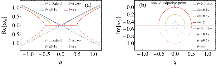
Figure S7: The Real (a) and imaginary (b) parts of the eigenvalues of the effective non-Hermitian system for the Rice-Mele model in the presence of loss difference. We have fixed $u=0$ and $\gamma=1$.

S4. Shockley Model in the Presence of Loss Difference

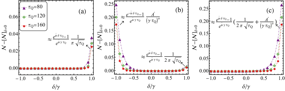
Figure S8: Scaled fermion density versus the variable $\delta/\gamma$ for the Shockley model in the presence of loss difference. In the quench protocols, the on-site energy parameter $u$ is ramped from $u_{i}=2v+1$ to $u_{f}=-(2v+1)$ in panel (a), from $u_{i}=0$ to $u_{f}=-(2v+1)$ in panel (b), and from $u_{i}=2v+1$ to $u_{f}=0$ in panel (c). We have selected the paraments, $w=v=1/2$ and $\gamma=\gamma_{a}+\gamma_{b}=0.1$ in the calculation.

The Shockley model is given by

$$H =\sum_{j}u\left(c_{a,j}^{\dagger}c_{a,j}-c_{b,j}^{\dagger}c_{b,j}\right)-\left(vc_{a,j}^{\dagger}c_{a,j+1}-vc_{b,j}^{\dagger}c_{b,j+1}+h.c.\right)-\left(wc_{a,j}^{\dagger}c_{b,j+1}-wc_{a,j+1}^{\dagger}c_{b,j}+h.c.\right).$$ (S77)

The linear quench protocol read $u(t)=u_{i}-\frac{t}{\tau_{Q}}$, which starts at $t_{i}=0$ and ends at $t_{f}=(u_{i}-u_{f})\tau_{Q}$. In the calculation, we have fixed the parameter $w=1/2$.

For the system coupled with loss difference governed by Eqs. (S26) and (S27), we get

$$\mathcal{N}\approx\left\{\begin{array}[]{cc}\frac{e^{\bar{u}\delta\tau_{Q}}-1}{e^{\bar{u}\gamma\tau_{Q}}}\frac{1}{\pi\sqrt{\tau_{Q}}}&(u_{i}>u_{c}>-u_{c}>u_{f});\\ \frac{e^{\bar{u}\delta\tau_{Q}}-1}{e^{\bar{u}\gamma\tau_{Q}}}\frac{1}{2\pi\sqrt{\tau_{Q}}}+\frac{e^{-\bar{u}\delta\tau_{Q}}-1}{e^{\bar{u}\gamma\tau_{Q}}}\frac{A^{{}^{\prime}}}{(\gamma\tau_{Q})^{\alpha}}&(u_{c}>u_{i}>-u_{c}>u_{f});\\ \frac{e^{\bar{u}\delta\tau_{Q}}-1}{e^{\bar{u}\gamma\tau_{Q}}}\{\frac{1}{2\pi\sqrt{\tau_{Q}}}+\frac{A^{{}^{\prime}}}{(\gamma\tau_{Q})^{\alpha}}\}&(u_{i}>u_{c}>u_{f}>-u_{c}),\end{array}\right.$$ (S78)

for large enough $\tau_{Q}$, as illustrated in Fig. (S8).

S5. DKZ Scaling Law in the Qi-Wu-Zhang Model

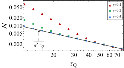
Figure S9: Fermion density as a function $\tau_{Q}$ for the Qi-Wu-Zhang model in the presence of LLD ($\gamma_{a}=\gamma$ and $\gamma_{b}=0$). We have selected paraments, $u_{i}=3$ and $u_{f}=-3$. The numerical solutions indicated by the colored dingbats collapse to the DKZ scaling law denoted by the black line consistently.

In Frouier space, the Qi-Wu-Zhang model is given by

$$H=\sum_{q}\left(\begin{array}[]{cc}c_{\uparrow,q}^{\dagger}&c_{\downarrow,q}^{\dagger}\end{array}\right)\left(\begin{array}[]{cc}u+\cos q_{x}+\cos q_{y}&\sin q_{x}-i\sin q_{y}\\ \sin q_{x}+i\sin q_{y}&-(u+\cos q_{x}+\cos q_{y})\end{array}\right)\left(\begin{array}[]{c}c_{\uparrow,q}\\ c_{\downarrow,q}\end{array}\right).$$ (S79)

The system exhibits three gapless points: the first one at $u=u_{c}=-2$ with a critical momentum $(q_{x}^{c},q_{y}^{c})=(0,0)$, the second one at $u=u_{c}=0$ with the critical momentum $(q_{x}^{c},q_{y}^{c})=(0,\pm\pi)$ and $(\pm\pi,0)$, and the last one at $u=u_{c}=2$ with the critical momentum $(q_{x}^{c},q_{y}^{c})=(\pm\pi,\pm\pi)$. When coupled with loss, the system is described by the Lindblad equation in Eq. (S26), but the loss term becomes

$$\mathcal{D}_{q}[\rho_{q}]= \gamma_{a}\left(c_{\uparrow,q}\rho_{q}c_{\uparrow,q}^{\dagger}-\frac{1}{2}\{\rho_{q},c_{\uparrow,q}^{\dagger}c_{\uparrow,q}\}\right)+\gamma_{b}\left(c_{\downarrow,q}\rho_{q}c_{\downarrow,q}^{\dagger}-\frac{1}{2}\{\rho_{q},c_{\downarrow,q}^{\dagger}c_{\downarrow,q}\}\right).$$ (S80)

The on-site energy parameter is linearly ramped across the quantum phase transition point as

$$u=u(t)=u_{i}-\frac{t}{\tau_{Q}}~{}~{}~{}(0\leq t\leq t_{f}).$$ (S81)

where we have $u_{i}\geq u_{c}>-u_{c}\geq u_{f}=u(t_{f})$. At the final time of the quench, the fermion density complies with the DKZ scaling law,

$$\mathcal{N}=\mathcal{N}_{\downarrow}+\mathcal{N}_{\uparrow}=\frac{1}{N}\sum_{q}(\text{Tr}(\rho c_{\downarrow,q}^{\dagger}c_{\downarrow,q})+\text{Tr}(\rho c_{\uparrow,q}^{\dagger}c_{\uparrow,q}))\approx\mathcal{N}_{\text{DKZ}}=\frac{1}{\pi^{2}\tau_{Q}},$$ (S82)

for large enough $\tau_{Q}$. As depicted in Fig. (S9), the analytical solution and numerical results are in good agreement.

References

- [1] S. Sachdev, Quantum Phase Transitions, 2nd ed (Cambridge University Press, 2011.).
- Kibble [1976] T. W. B. Kibble, J. Phys. A 9, 1387 (1976).
- Zurek [1985] W. H. Zurek, Nature 317, 505 (1985).
- Zurek et al. [2005] W. H. Zurek, U. Dorner, and P. Zoller, Phys. Rev. Lett. 95, 105701 (2005).
- Dziarmaga [2005] J. Dziarmaga, Phys. Rev. Lett. 95, 245701 (2005).
- Polkovnikov [2005] A. Polkovnikov, Phys. Rev. B 72, 161201 (R) (2005).
- Damski and Zurek [2006] B. Damski and W. H. Zurek, Phys. Rev. A 73, 063405 (2006).
- Uhlmann et al. [2007] M. Uhlmann, R. Schützhold, and U. R. Fischer, Phys. Rev. Lett. 99, 120407 (2007).
- Dziarmaga [2010] J. Dziarmaga, Advances in Physics 59, 1063 (2010).
- Polkovnikov et al. [2011] A. Polkovnikov, K. Sengupta, A. Silva, and M. Vengalattore, Rev. Mod. Phys. 83, 863 (2011).
- Kou and Li [2022] H.-C. Kou and P. Li, Phys. Rev. B 106, 184301 (2022).
- Kou and Li [2023] H.-C. Kou and P. Li, Phys. Rev. B 108, 214307 (2023).
- Liou and Yang [2018] S.-F. Liou and K. Yang, Phys. Rev. B 97, 235144 (2018).
- Ulčakar et al. [2020] L. Ulčakar, J. Mravlje, and T. c. v. Rejec, Phys. Rev. Lett. 125, 216601 (2020).
- Bandyopadhyay and Dutta [2020] S. Bandyopadhyay and A. Dutta, Phys. Rev. B 102, 184302 (2020).
- Sun et al. [2022] Z. Sun, M. Deng, and F. Li, Phys. Rev. B 106, 134203 (2022).
- Cooper et al. [2019] N. R. Cooper, J. Dalibard, and I. B. Spielman, Rev. Mod. Phys. 91, 015005 (2019).
- Liang et al. [2023] M.-C. Liang, Y.-D. Wei, L. Zhang, X.-J. Wang, H. Zhang, W.-W. Wang, W. Qi, X.-J. Liu, and X. Zhang, Phys. Rev. Res. 5, L012006 (2023).
- Breuer and Petruccione [2002] H.-P. Breuer and F. Petruccione, The Theory of Open Quantum Systems (Oxford University Press, 2002).
- Griffin et al. [2012] S. M. Griffin, M. Lilienblum, K. T. Delaney, Y. Kumagai, M. Fiebig, and N. A. Spaldin, Phys. Rev. X 2, 041022 (2012).
- Dutta et al. [2016] A. Dutta, A. Rahmani, and A. del Campo, Phys. Rev. Lett. 117, 080402 (2016).
- Gao et al. [2017] Z.-P. Gao, D.-W. Zhang, Y. Yu, and S.-L. Zhu, Phys. Rev. B 95, 224303 (2017).
- Ai et al. [2021] M.-Z. Ai, J.-M. Cui, R. He, Z.-H. Qian, X.-X. Gao, Y.-F. Huang, C.-F. Li, and G.-C. Guo, Phys. Rev. A 103, 012608 (2021).
- Singh and Gangadharaiah [2021] M. Singh and S. Gangadharaiah, Phys. Rev. B 104, 064313 (2021).
- Singh et al. [2023] M. Singh, S. Dhara, and S. Gangadharaiah, Phys. Rev. B 107, 014303 (2023).
- Bandyopadhyay et al. [2018] S. Bandyopadhyay, S. Laha, U. Bhattacharya, and A. Dutta, Sci. Rep 8, 11921 (2018).
- Puebla et al. [2020] R. Puebla, A. Smirne, S. F. Huelga, and M. B. Plenio, Phys. Rev. Lett. 124, 230602 (2020).
- Rossini and Vicari [2020] D. Rossini and E. Vicari, Phys. Rev. Res. 2, 023211 (2020).
- King et al. [2023] E. C. King, J. N. Kriel, and M. Kastner, Phys. Rev. Lett. 130, 050401 (2023).
- Arceci et al. [2018] L. Arceci, S. Barbarino, D. Rossini, and G. E. Santoro, Phys. Rev. B 98, 064307 (2018).
- Bacsi and Dora [2023] A. Bacsi and B. Dora, Sci. Rep 13, 4034 (2023).
- Juhász and Roósz [2023] R. Juhász and G. m. H. Roósz, Phys. Rev. B 108, 224203 (2023).
- Jara and Cosme [2024] R. D. Jara and J. G. Cosme, Phys. Rev. B 110, 064317 (2024).
- Ding and Zhang [2024] C. Ding and L. Zhang, Universal quench dynamics of an open quantum system (2024), arXiv:2408.04329 .
- Houck et al. [2012] A. A. Houck, H. E. Türeci, and J. Koch, Nature Physics 8, 292 (2012).
- Fitzpatrick et al. [2017] M. Fitzpatrick, N. M. Sundaresan, A. C. Y. Li, J. Koch, and A. A. Houck, Phys. Rev. X 7, 011016 (2017).
- Bernien et al. [2017] H. Bernien, S. Schwartz, A. Keesling, and H. Levine, Nature 551, 579 (2017).
- Aspelmeyer et al. [2014] M. Aspelmeyer, T. J. Kippenberg, and F. Marquardt, Rev. Mod. Phys. 86, 1391 (2014).
- Gil-Santos et al. [2017] E. Gil-Santos, M. Labousse, C. Baker, A. Goetschy, W. Hease, C. Gomez, A. Lemaître, G. Leo, C. Ciuti, and I. Favero, Phys. Rev. Lett. 118, 063605 (2017).
- Verstraete et al. [2009] F. Verstraete, M. M. Wolf, and J. Ignacio Cirac, Nature Physics 5, 633 (2009).
- Tóth et al. [2017] L. Tóth, N. Bernier, A. Nunnenkamp, A. Feofanov, and T. Kippenberg, Nature Physics 13, 787 (2017).
- Ren et al. [2022] Z. Ren, D. Liu, E. Zhao, C. He, K. K. Pak, J. Li, and G.-B. Jo, Nature Physics 18, 385 (2022).
- Feng et al. [2023] Y. Feng, Z. Liu, F. Liu, J. Yu, S. Liang, F. Li, Y. Zhang, M. Xiao, and Z. Zhang, Phys. Rev. Lett. 131, 013802 (2023).
- Kholodenko and Silagadze [2012] A. L. Kholodenko and Z. K. Silagadze, Physics of Particles and Nuclei 43, 882 (2012).
- Kenmoe et al. [2013] M. B. Kenmoe, H. N. Phien, M. N. Kiselev, and L. C. Fai, Phys. Rev. B 87, 224301 (2013).
- [46] See Supplemental Material for two-band models in the presence of loss (S1), dissipative critical dynamics of the Rice-Mele model (S2), the effective non-Hermitian system with loss difference for the Rice-Mele model (S3), Shockley model in the presence of loss difference (S4), and DKZ scaling law in Qi-Wu-Zhang model (S5). References [9, 26, 28, 44, 45] are included.
- McCann [2023] E. McCann, Phys. Rev. B 107, 245401 (2023).
- Asbóth et al. [2016] J. K. Asbóth, L. Oroszlány, and A. Pályi, A Short Course on Topological Insulators (Springer, 2016).
- Haldane [1988] F. D. M. Haldane, Phys. Rev. Lett. 61, 2015 (1988).
- Shen [2017] S.-Q. Shen, Topological Insulators (Springer, 2017).
- Li et al. [2023] Y. Li, C. Lu, S. Zhang, and Y.-C. Liu, Phys. Rev. B 108, L220301 (2023).
- Qi et al. [2006] X.-L. Qi, Y.-S. Wu, and S.-C. Zhang, Phys. Rev. B 74, 085308 (2006).
- B. S et al. [2020] R. B. S, V. Mukherjee, U. Divakaran, and A. del Campo, Phys. Rev. Res. 2, 043247 (2020).