Large Deviations of Cover Time of Tori in Dimensions $d\geq 3$

Abstract

We consider large deviations of the cover time of the discrete torus $(\mathbb{Z}/N\mathbb{Z})^{d}$, $d\geq 3$ by simple random walk. We prove a lower bound on the probability that the cover time is smaller than $\gamma\in(0,1)$ times its expected value, with exponents matching the upper bound from [18] and [12]. Moreover, we derive sharp asymptotics for $\gamma\in(\frac{d+2}{2d},1)$. The strong coupling of the random walk on the torus and random interlacements developed in a recent work [25] serves as an important ingredient in the proofs.

0 Introduction

The cover time of a Markov chain is a natural mathematical concept that finds many applications in probability theory, combinatorics and theoretical computer science. In particular, cover times by simple random walk on tori have been studied extensively. For $d\geq 3$, asymptotics and Gumbel fluctuation of cover times are given in [3, Chapter 7.2.2], and [6] respectively. For the much harder $d=2$ case, the works [14], [7] (see also [2]) and [8] give precise first- and second-order asymptotics and the tightness of the third-order fluctuation respectively.

Intimately related to the cover time is the structure of late points or avoided points. We refer readers to [1] for a survey on this topic. In particular, for $d\geq 3$, [6] and [23] prove the uniformity of the late points on torus and more recently in [25], a very strong coupling of the trace of random walk and random interlacements is obtained, yielding a structural characterization of the late points.

In this article, we focus on large deviations of the cover time of the $d$-dimensional discrete torus, $d\geq 3$. Let $X=(X_{n})_{n\geq 0}$ be a discrete-time simple random walk on the $d$-dimensional torus $\mathbb{T}_{N}=(\mathbb{Z}/N\mathbb{Z})^{d}$ for $d\geq 3$ and $\mathsf{P}$ be the law (and $\mathsf{E}$ the respective expectation) of the walk starting from the uniform distribution. The cover time $\mathfrak{C}_{N}$ is the first time $X$ has visited every vertex of the torus. For $d\geq 3$, it is classical that

(0.1) $$\mathsf{E}{\mathfrak{C}_{N}}\sim t_{\operatorname{cov}}\overset{\text{def.}}{=}g(0)N^{d}\log N^{d},\text{ as }N\to\infty,$$

where $g(\cdot)$ denotes Green’s function on $\mathbb{Z}^{d}$. In [6], finer asymptotics on $\mathfrak{C}_{N}$ are obtained:

$$\mathfrak{C}_{N}/(g(0)N^{d})-\log N^{d}\Longrightarrow\mbox{Gumbel distribution as }N\to\infty.$$

An upper bound (on the cover probability) is established for the $\varepsilon$-cover time of a torus by Brownian motion in dimensions $d\geq 3$; see [18, Corollary 1.9]. As noted in [12], the proof can be adapted to the discrete setting, yielding an upper bound with a conjecturally correct exponent; see (0.6) below for the precise statement. In the 2D case, the correct order is obtained in [12] with the help of soft local time techniques introduced in [24] in the upper bound and a covering strategy (which fails in higher dimensions) for the lower bound, but sharp asymptotics remain open. We also remark that for even larger deviations at the order of the volume of torus, the general result “linear cover time is exponentially unlikely” applies (see [9, 16]), but it remains a hard problem to determine a sharp decay rate in this regime.

We now state our main results. For $\gamma\in(\gamma_{0},1)$, where

(0.2) $$\gamma_{0}\overset{\text{def.}}{=}\frac{d+2}{2d},$$

we give sharp asymptotics of the probability of the event

(0.3) $$U_{\gamma,N}\overset{\text{def.}}{=}\big{\{}\mathfrak{C}_{N}\leq\gamma t_{\operatorname{cov}}\big{\}}$$

that the cover time falls below a proportion of its expectation:

Theorem 0.1.

For $\gamma\in(\gamma_{0},1)$,

(0.4) $$\lim_{N\to\infty}\frac{\log\mathsf{P}\big{(}U_{\gamma,N}\big{)}}{N^{d(1-\gamma)}}=-1.$$

The method we use to prove the lower bound in Theorem 0.1 can also be applied to obtain the following lower bound for the whole range of $\gamma\in(0,1)$:

Theorem 0.2.

There exists a constant $C>0$ such that for all $\gamma\in(0,1)$,

(0.5) $$\mathsf{P}\big{(}U_{\gamma,N}\big{)}\geq\exp\Big{(}-C\cdot N^{d(1-\gamma)}\Big{)}.$$

As discussed above, the deviation probability admits a rough upper bound:

(0.6) $$\mathsf{P}\big{(}U_{\gamma,N}\big{)}\leq\exp\Big{(}-N^{d(1-\gamma)+o(1)}\Big{)}\quad\mbox{ for all }\gamma\in(0,1).$$

For completeness we will sketch a proof of (0.6) in the Appendix. Theorem 0.2 and (0.6) immediately imply the following asymptotics.

Corollary 0.3.

For all $\gamma\in(0,1)$,

$$\mathsf{P}\big{(}U_{\gamma,N}\big{)}=\exp\Big{(}-N^{d(1-\gamma)+o(1)}\Big{)}.$$

We also state below asymptotics of the upward deviation probability: for $\gamma>1$,

(0.7) $$\mathsf{P}\big{(}\mathfrak{C}_{N}\geq\gamma t_{\operatorname{cov}}\big{)}=\big{(}1+o(1)\big{)}N^{-d(\gamma-1)}.$$

Although (0.7) is a straightforward application of moment bounds, a sketch of proof will still be provided in Remark 2) for completeness.

0.1 Proof overview and discussion

A powerful tool for analyzing the behavior of simple random walk in three and higher dimensions is the model of random interlacements first introduced in [26]. It is a Poissonian cloud of bi-infinite random walk trajectories. Random interlacements naturally appear in the local limit of the trace of a simple random walk on a large torus when it runs up to a time proportional to its volume. Several coupling results between random walks on torus and random interlacements have been established; see e.g. [32, 31, 6, 33, 25]. In particular, [6] considers the excursions between two concentric cubes to establish a coupling result at a mesoscopic scale. Using the soft local times method introduced in [24], [33] constructs a coupling at a macroscopic scale. The soft local times method is further refined in [25], leading to a stronger coupling result with an explicit error term, namely [25, Theorem 5.1] (paraphrased in this article as Proposition 1.5), which is a key ingredient in this article. The notion corresponding to cover time for interlacements is called the cover level and has been studied in detail in [5].

We will now briefly outline the proof of Theorem 0.1. We begin with notation. For $\alpha\in(0,1)$, let $\mathcal{L}^{\alpha}$ denote the set of uncovered sites up to time $\alpha g(0)N^{d}\log N^{d}$. The elements of $\mathcal{L}^{\alpha}$ will be referred to as $\alpha$-late points, or simply late points if $\alpha$ can be specified from the context. To better indicate the level parameter of random interlacements to be coupled with the random walk, for $\gamma>0$, we write

(0.8) $$u_{N}(\gamma)\overset{\text{def.}}{=}\gamma g(0)\log N^{d}\quad\mbox{ and }\quad u_{N}=u_{N}(1).$$

Note that $u_{N}(\gamma)N^{d}=\gamma t_{\operatorname{cov}}$.

We first discuss the upper bound. We divide (the bulk of) $\mathbb{T}_{N}$ into cubes of side-length $N^{\gamma}$ which are $\delta N^{\gamma}$ away from each other, where $\delta>0$ is a small quantity to be sent to $0$ eventually. By Corollary 1.6, a coupling result derived from [25, Theorem 5.1], we obtain that with high probability the trace of random walk up to $\gamma t_{\operatorname{cov}}$ intersected with these cubes can be dominated by independent random interlacements with intensity slightly bigger than $u_{N}(\gamma)$. Moreover, our choice of side-length of the cubes ensures that the typical cover level of each cube is approximately $u_{N}(\gamma)$, so the probability for the random interlacements to cover each cube ($\approx\mathrm{e}^{-1}$ thanks to [5, Theorem 0.1]) is determined by the asymptotics of the cover level. Combining the two facts gives the desired bound.

We now turn to the more delicate lower bound. For the lower bound in Theorem 0.1, we summarize our four-stage strategy as follows:

Stage 1: Let the random walk roam freely until

$$T_{1}\overset{\text{def.}}{=}\lfloor\alpha_{N}t_{\operatorname{cov}}\rfloor,\quad\mbox{with}\quad\alpha_{N}\overset{\text{def.}}{=}\gamma-KN^{d}/t_{\operatorname{cov}},\;\mbox{for some large }K.$$

This choice of $T_{1}$ ensures that the typical number of late points is of order $N^{d(1-\gamma)}$; see Section 1.3 for moment bounds on late points. Some specific uniformity requirements of the late points $\mathcal{L}^{\alpha_{N}}$ (see (3.7) for precise statements) are also typically satisfied; see Lemma 3.4.

Stage 2: We divide $\mathbb{T}_{N}$ into the “bulk” part and the “edge” part, with the former isomorphic to $Q(0,(1-\delta)N)\subset\mathbb{Z}^{d}$, a $d$-dimensional cube of side-length $(1-\delta)N$ (see (1.1) for definition), with some small $\delta>0$. We then apply the coupling Proposition 1.5 in the bulk to show that the probability that the points of $\mathcal{L}^{\alpha_{N}}$ in the bulk are covered between $T_{1}$ and $T_{2}$, where

$$T_{2}\overset{\text{def.}}{=}\lfloor\beta_{N}t_{\operatorname{cov}}\rfloor,\quad\mbox{with}\quad\beta_{N}\overset{\text{def.}}{=}\gamma-5\varepsilon N^{d}/t_{\operatorname{cov}}\;\mbox{ (for some small }\varepsilon>0),$$

exceeds $\exp\big{(}-(1+\eta)N^{d(1-\gamma)}\big{)}$ for a small $\eta=\eta(\delta,\varepsilon)>0$ (to be sent to $0$ eventually) by turning the estimate on the cover probability in the bulk into a cover-level large deviation probability estimate for random interlacements and by benefiting from Harris-FKG inequality for Poisson point processes. See Proposition 3.1 for the precise statement. Restricting $\gamma$ to $(\gamma_{0},1)$ ensures that the coupling error is ignorable even with respect to the cover probability.

Stage 3: We perform “surgeries” on the trace of random walk between $T_{2}$ and

$$T_{3}\overset{\text{def.}}{=}\lfloor\gamma t_{\operatorname{cov}}-\varepsilon N^{d}\rfloor$$

by inserting meticulously designed loops into the trajectory in a specific fashion (see Section 4 for details) to cover points of $\mathcal{L}^{\alpha_{N}}$ in the edge part. For paths that are “nice” during Stage 1 and satisfy some extra requirements (see Definition 3.2 for details), the total length of these loops is bounded by a constant times the number of late points, which does not exceed $\varepsilon N^{d}$; see Lemma 4.9 for a precise statement. Moreover, the whole loop-insertion mechanism is designed in a way so that it is possible to recover the original trajectory deterministically from the trajectory after insertion; see Proposition 4.1, in particular (4.1c), for details. This allows us to establish a lower bound on the probability that the late points in the edge is covered after $T_{2}$; see Proposition 3.3 for details.

Stage 4: We again let the random walk roam freely until $T_{4}\overset{\text{def.}}{=}\lfloor\gamma t_{\operatorname{cov}}\rfloor$. Note that the bound on the total length of the loops ensures that there is still time left after loop-insertion surgeries.

To establish Theorem 0.2, we skip Stage 2 in the strategy above and proceed to loop insertion directly to cover late points at the end of Stage 1. As no coupling with random interlacements is involved, such a strategy works for all $\gamma\in(0,1)$, but yields only a lower bound that is sub-optimal in the pre-factor; see Section 3.3 for details.

We now make a few remarks on the proof strategy and a few related problems.

We first compare our strategy with that of the 2D case treated in [12]. Both proofs crucially rely on “soft local time” techniques first introduced in [24] to decouple trace of random walk. However, thanks to the Bernoulli nature of late points (see [25] for more discussions) for $d\geq 3$, in our case we are able to obtain a sharp asymptotic deviation probability (for at least large values of $\gamma$), while obtaining sharp asymptotics for 2D deviation probability remains a difficult question. For the upper bounds, in both cases a decoupling of the trace of random walk in mesoscopic cubes is involved. However, in the 2D case, boxes of a different side-length are chosen and the trace of random walk are approximated by collection of random walk excursions instead of interlacements. For lower bounds the strategy employed in either case is very specific and not easily adaptable to the other case; see also the discussions in Section 1 of [12].

It is worth noting that similar sharp asymptotics can be obtained for a counterpart problem regarding random interlacements which is reminiscent of the “hard-wall” conditioning of Gaussian free field [11, 10]. More precisely, let $\mathcal{I}^{u}$ stand for the interlacement set at level $u>0$ (see Section 1.1 for precise definitions), and $\mathfrak{M}_{N}=\inf\{u\geq 0:Q(0,N)\subset\mathcal{I}^{u}\}$ for the cover level of the $d$-dimensional cube $Q(0,N)$ of side-length $N$. It is possible to establish that

(0.9) $$\mathbb{P}(\mathfrak{M}_{N}\leq\gamma u_{N})=\exp\left(-(1+o(1))N^{d(1-\gamma)}\right),\qquad\mbox{for all }\gamma\in\left(\frac{d}{2d-2},1\right).$$

The lower bound in (0.9) (which actually works for all $\gamma\in(0,1)$) follows readily from the Harris-FKG inequality for random interlacements. For the upper bound, we again divide $Q(0,N)$ into cubes of side-length $N^{\gamma}$ with $\delta N^{\gamma}$ space in-between and apply [25, Theorem 5.1] to localize random interlacements, akin to the proof of upper bound in Theorem 0.1. Thanks to a better error bound for interlacements developed in [25, Theorem 5.1] (see also Proposition 1.4 in our work; readers may compare (1.13) and (1.14) therein), the proof strategy can work for a larger range of $\gamma$ than the case of random walk.

However, when $\gamma\in(0,\frac{2}{d})$, another strategy involving the so-called “tilted interlacements” kicks in, and changes the asymptotics completely. We now briefly explain this strategy. To study the asymptotic probability that random interlacements with low intensity disconnects a macroscopic body from infinity, the authors of [22] introduce a Markov jump process with a specific spatially-regulated local drift towards $Q(0,N)$ and construct a spatially inhomogeneous variant of random interlacements (which they name by tilted interlacements) with the aforementioned Markov process serving as the underlying random walk in the construction of interlacements. In a neighborhood of $Q(0,N)$, tilted interlacements (locally) look like random interlacements of an uplifted intensity. By imitating the calculation in [22] on the relative entropy between tilted interlacements and standard interlacements, one arrives at the following lower bound:

(0.10) $$\mathbb{P}(\mathfrak{M}_{N}\leq\gamma u_{N})\geq\exp\left(-\big{(}(\sqrt{\gamma}-1)^{2}g(0){\rm cap}_{\mathbb{R}^{d}}([0,1]^{d})+o(1)\big{)}N^{d-2}\log N\right)$$

where ${\rm cap}_{\mathbb{R}^{d}}(\cdot)$ stands for the Brownian capacity. It is a very interesting question whether one can apply some coarse-graining strategy to show that the RHS of (0.10) is actually sharp. We refer to [27, 28, 29] for applications of such strategies to derive sharp asymptotic upper bounds of disconnection, apparition of macroscopic holes and bulk deviation probabilities for interlacements.

For a simple random walk $(Y_{n})_{n\geq 0}$ on $\mathbb{Z}^{d}$, by employing a strategy involving “tilted walk” first introduced in [21], which resembles to some extent the strategy described above, a similar asymptotic lower bound for the probability that $Y_{n}$ covers the macroscopic cube $Q(0,N)$ emerges:

(0.11) $$\mathsf{P}_{0}\big{(}Q(0,N)\subset Y_{[0,\infty)}\big{)}\geq\exp\left(-\big{(}g(0){\rm cap}_{\mathbb{R}^{d}}([0,1]^{d})+o(1)\big{)}N^{d-2}\log N\right).$$

If RHS of (0.10) is sharp, then by a natural coupling of $Y_{[0,\infty)}$ and $\mathcal{I}^{u}$ conditioned on $0\in\mathcal{I}^{u}$ (see the paragraph above [27, (1.8)] for a similar argument) for arbitrarily small $u>0$, the RHS of (0.11) is also sharp. However, it should be noted that such a strategy fails to work for the original problem, as it does not involve a constraint on the total time spent in $Q(0,N)$. This strongly suggests that idea of coupling random walk with interlacements is not suitable for treating the case $\gamma\in(0,\frac{2}{d})$ and a new strategy is required.

Before ending this subsection, we briefly mention a “dual” problem of what we consider in this work, namely the downward large deviation of maximal local time for simple random walk on $\mathbb{Z}^{d}$ for $d\geq 3$. For simplicity we restrict to discrete-time walks. We still let $(Y_{n})_{n\geq 0}$ stand for the simple random walk on $\mathbb{Z}^{d}$, $d\geq 3$. Let $\xi(x,n)$ be its local-time process at site $x\in\mathbb{Z}^{d}$ at time $n\geq 0$ and $\xi^{*}(n):=\max_{x\in\mathbb{Z}^{d}}\xi(x,n)$ the maximal local time at time $n$, respectively. It is classical (see [17, Theorem 1.3]) that

(0.12) $$\lim_{N\to\infty}\frac{\xi^{*}(N)}{\log N}=\alpha:=-\frac{1}{\log(1-{\rm Es}_{d})},$$

where ${\rm Es}_{d}:=\mathsf{P}_{0}[0\notin Y_{(1,\infty)}]$ is the escape probability. An interesting question is, for any $d\geq 3$ and all $\gamma\in(0,1)$, does one have

(0.13) $$\mathsf{P}\big{(}\xi^{*}(N)\leq\gamma\cdot\alpha\log N\big{)}=\exp\Big{(}-N^{1-\gamma+o(1)}\Big{)}?$$

Moreover, does sharp asymptotics similar to (0.4) also hold? More precisely, for all $d\geq 3$ does there exist a $C=C(d)>0$ (possibly $\equiv 1$) such that for all $\gamma\in(\gamma^{\prime}_{0},1)$ for some $\gamma^{\prime}_{0}=\gamma^{\prime}_{0}(d)<1$,

(0.14) $$P\big{(}\xi^{*}(N)\leq\gamma\cdot\alpha\log N\big{)}=\exp\Big{(}-\big{(}C+o(1)\big{)}N^{1-\gamma}\Big{)}?$$

A simple strategy of chopping $Y_{[0,N]}$ into segments of length $N^{\gamma}$ yields an upper bound for both (0.13) and (0.14). It would be very nice to develop a matching sharp lower bound for a largest possible range of $\gamma$.

0.2 Organization of this article

Section 1 introduces the relevant notation, briefly discusses the model of random interlacements and its connection with random walks, and presents moment bounds and concentration results for late points. Section 2 establishes the upper bound in Theorem 0.1. Section 3 demonstrates the lower bounds for Theorem 0.1 and Theorem 0.2. Section 4 is dedicated to the surgery of loop-insertion for the lower bounds. Its main goal is the proof of Proposition 3.3, which is relatively independent of other materials in Section 3. Appendix A sketches the proof of (0.6), the rough upper bound.

We conclude this section with our convention regarding constants. In the rest of the article, constants without numeric subscripts may vary from place to place, while constants with numeric subscripts remain fixed within the same section. All constants depend implicitly on the dimension $d$. Unless stated otherwise, all constants are positive.

Acknowledgments: The authors thank the support of National Key R&D Program of China (No. 2021YFA1002700 and No. 2020YFA0712900) and NSFC (No. 12071012).

1 Notation and preliminaries

We first set up some basic notation. For any positive sequence $(a_{N})_{N\geq 0}$, we say $a_{N}=o(1)$ if $\lim_{N\to\infty}a_{N}=0$. Given two positive functions $f$ and $g$, we write $f\sim g$ if $\lim\frac{f}{g}=1$, where the limiting process can be inferred from the context. For any $a\in\mathbb{R}$, let $\lfloor a\rfloor$ denote the greatest integer less than or equal to $a$, and $\lceil a\rceil$ denote the smallest integer greater than or equal to $a$.

We use $\phi_{N}$ to denote the canonical map from the lattice $\mathbb{Z}^{d}$ to the torus $\mathbb{T}_{N}$. For convenience, we always use $\boldsymbol{x}$ to denote the projection image $\phi_{N}(x)$ for $x\in\mathbb{Z}^{d}$. The addition and subtraction of vectors on $\mathbb{T}_{N}$ are addition and subtraction modulo $n$ in each coordinate. For $x\in\mathbb{Z}^{d}$ and $R>0$, we let $Q(x,R)=x+([-\lfloor(R-1)/2\rfloor,\lceil(R-1)/2\rceil]\cap\mathbb{Z})^{d}$ be the cube of side-length $R$ around $x$ in $\mathbb{Z}^{d}$, and $Q(\boldsymbol{x},R)=\phi_{N}(Q(x,R))$ be the cube in the torus. For brevity, we also write

(1.1) $$Q_{R}(x)=Q(x,R),\qquad Q_{\delta}=Q(0,(1-\delta)N)\qquad\mbox{ and }\qquad\boldsymbol{Q}_{\delta}=Q(\boldsymbol{0},(1-\delta)N).$$

We write $\varphi_{N}=\phi_{N}\mid_{Q(0,N)}$ for the bijection from $Q(0,N)$ to $\mathbb{T}_{N}$.

For $x\in\mathbb{Z}^{d}$, we use $|x|_{\infty}$ and $|x|_{1}$ to denote the $l^{\infty}$ norm and the $l^{1}$ norm respectively. With slight abuse of notation, we also use them to denote the induced norms on $\mathbb{T}_{N}$. For clarity, we let $d_{\infty}(x,y)=|x-y|_{\infty}$ and $d_{1}(x,y)=|x-y|_{1}$ for $x,y\in\mathbb{Z}^{d}$ (or $\mathbb{T}_{N}$). For $x\in\mathbb{T}_{N}$ and $K\subset\mathbb{T}_{N}$ (or $x\in\mathbb{Z}^{d}$ and $K\subset\mathbb{Z}^{d}$), we write $d_{\infty}(x,K)=\min\{d_{\infty}(x,y):y\in K\}$ for the $l^{\infty}$-distance from $x$ to $K$. Write $e_{1}=(1,0,\ldots,0)$ and define $e_{2},\ldots,e_{d}$ similarly.

We write $\mathsf{P}_{x}$ for the canonical law of the discrete-time simple random walk on $\mathbb{Z}^{d}$ (or $\mathbb{T}_{N}$, depending on context) starting at $x\in\mathbb{Z}^{d}$ (or $\mathbb{T}_{N}$). Let $\mathsf{P}=N^{-d}\sum_{x\in\mathbb{T}_{N}}\mathsf{P}_{x}$ be the law of the random walk starting from the uniform distribution on $\mathbb{T}_{N}$. We also write $\mathsf{E}$ or $\mathsf{E}_{x}$ for the expectation under $\mathsf{P}$ or $\mathsf{P}_{x}$ respectively. We denote by $(X_{n})_{n\geq 0}$ the corresponding random walk process under $\mathsf{P}_{x}$ or $\mathsf{P}$, and by $X\langle t_{1},t_{2}\rangle=\{X_{n}:n\in\langle t_{1},t_{2}\rangle\}$ the trace left by the random walk from time $t_{1}$ to $t_{2}$, where $\langle\in\{(,[\}$ and $\rangle\in\{),]\}$. We write $\mathcal{F}_{n}$ for the natural filtration generated by $(X_{k})_{0\leq k\leq n}$.

For $k\in\mathbb{N}$, we write

(1.2) $$\Omega_{\boldsymbol{x},k}=\{(\boldsymbol{x}_{0},\boldsymbol{x}_{1},\ldots,\boldsymbol{x}_{k})\subset(\mathbb{T}_{N})^{k}:\boldsymbol{x}_{0}=\boldsymbol{x},\,|\boldsymbol{x}_{i}-\boldsymbol{x}_{i-1}|_{1}=1\text{ for all }1\leq i\leq k\}$$

for the collection of all possible trajectories of random walk on $\mathbb{T}_{N}$ started from $\boldsymbol{x}$ up to time $k$. We also write $\Omega_{k}=\bigcup_{\boldsymbol{x}\in\mathbb{T}_{N}}\Omega_{\boldsymbol{x},k}$ for all possible random walk trajectories up to time $k$ and $\Omega=\bigcup_{k\in\mathbb{N}}\Omega_{k}$ for the collection of trajectories of finite length. For a path $\omega\in\Omega_{k}$, we let $L(\omega)=k$ be the length of $\omega$. Moreover, for two paths $\omega,\omega^{\prime}\in\Omega$ and $0\leq t_{1}\leq t_{2}\leq\min\{L(\omega),L(\omega^{\prime})\}$, we write $\omega=\omega^{\prime}\mid_{[t_{1},t_{2}]}$ if $\omega(k)=\omega^{\prime}(k)$ for all $t_{1}\leq k\leq t_{2}$. For simplicity, we write $\omega=\omega^{\prime}\mid_{t_{1}}$ for $\omega=\omega^{\prime}\mid_{[0,t_{1}]}$. For $k\in\mathbb{N}$, we define a map $\pi_{k}$ from events in $\mathcal{F}_{k}$ to related random walk paths of length $k$:

(1.3) $$\pi_{k}(A)=\left\{\omega=(\boldsymbol{x}_{0},\boldsymbol{x}_{1},\ldots,\boldsymbol{x}_{k})\subset\Omega_{k}\mid\{X_{\cdot}=\omega\mid_{k}\}\subset A\right\},\quad\text{for }A\in\mathcal{F}_{k}.$$

For $K\subset\mathbb{Z}^{d}$ or $\mathbb{T}_{N}$, we define $H_{K}=\inf\{n\geq 0:X_{n}\in K\}$ and $\widetilde{H}_{K}=\inf\{n\geq 1:X_{n}\in K\}$ the respective entrance time and hitting time of $K$. We write $H_{x}$ and $\widetilde{H}_{x}$ for $H_{\{x\}}$ and $\widetilde{H}_{\{x\}}$ respectively. Let $\mathfrak{C}_{N}=\max_{x\in\mathbb{T}_{N}}H_{x}$ be the cover time of the torus $\mathbb{T}_{N}$.

For a finite $K\subset\mathbb{Z}^{d}$, we write $e_{K}(\cdot)$ for the equilibrium measure of $K$,

$$e_{K}(x)=\mathsf{P}_{x}(\widetilde{H}_{K}=\infty)1_{K}(x),$$

which is supported on the internal boundary of $K$. We denote by $\operatorname{cap}(K)$ the total mass of $e_{K}$ and call it the capacity of $K$, and by $\overline{e}_{K}=\frac{e_{K}}{\operatorname{cap}(K)}$ the normalized equilibrium measure. For $K\subset\mathbb{T}_{N}$ with $l^{\infty}$-diameter $\delta(K)<N$, we define its capacity as follows: if $K\subset Q(\boldsymbol{0},N-1)$, we let $\operatorname{cap}(K)\overset{\text{def.}}{=}\operatorname{cap}\big{(}\phi_{N}^{-1}(K)\big{)}$ (see the definition of $\phi_{N}$ at the beginning of this section); for other $K$’s with $\delta(K)<N$, we define $\operatorname{cap}(K)$ by translation invariance. Asymptotics of capacity are well known, and we will use the following bounds (see e.g. [19, Section 2.2]),

(1.4) $$cR^{d-2}\leq\operatorname{cap}(Q(0,R))\leq CR^{d-2}\quad,N\geq 1.$$

For two vertices $x,y\in\mathbb{Z}^{d}$, we denote by $g(x,y)$ the Green’s function of $X$, the simple random walk on $\mathbb{Z}^{d}$, under $\mathsf{P}_{x}$. Write $g(x-y)\overset{\text{def.}}{=}g(x,y)$ for short. From [25, Lemma 2.1], we have for all integers $n\geq 0$,

(1.5) $$\sup_{|x|_{1}>n}g(x)<\sup_{|x|_{1}=n}g(x).$$

1.1 Random interlacements

In this section, we present a concise overview of the model of random interlacements on $\mathbb{Z}^{d}$. We refer readers to [15] for a more detailed introduction. Let $\omega$ denote the random interlacements process on $\mathbb{Z}^{d}$, with the law $\mathbb{P}$, as defined in [26]. This process is a Poisson point process (with a certain translation-invariant intensity measure) of bi-infinite random walk trajectories, each associated with a positive label. The trace of the trajectories with label less than $u>0$, called the interlacement set at level $u$, is denoted by $\mathcal{I}^{u}$. Its complement, the vacant set $\mathcal{V}^{u}$ at level $u$, satisfies the following characterization:

(1.6) $$\mathbb{P}(K\subset\mathcal{V}^{u})=\exp\{-u\operatorname{cap}(K)\}\mbox{ for any }K\subset\subset\mathbb{Z}^{d}.$$

In particular, one has (see e.g. [15, (1.3.7) and (1.3.8)])

(1.7) $$\mathbb{P}(x\in\mathcal{V}^{u})=\exp\Big{(}-\frac{u}{g(0)}\Big{)},$$

and

(1.8) $$\mathbb{P}(x,y\in\mathcal{V}^{u})=\exp\Big{(}-\frac{2u}{g(0)+g(x-y)}\Big{)}.$$

The next lemma gives an upper bound on sums of two-point probability for the vacant set which will be useful in bounding certain sums of two-point probability for late points of random walk; see the proof of Lemma 1.9 for details. It follows directly from [4, Lemma 1.5] by taking $a=N$ therein and noting that $|F|\leq(2N)^{d}$ if $F\subset Q(0,2N-1)$.

Lemma 1.1.

There exist constants $C>0$ and $c_{1}>1$ such that for all $u\geq 0$, $N\in\mathbb{N}$ and $F\subset Q(0,2N-1)$,

$$\sum_{v\in F}\mathbb{P}\Big{(}0,v\in\mathcal{V}^{g(0)u}\Big{)}\leq\mathrm{e}^{-2u}\big{(}|F|+CuN^{2}\big{)}+C\exp(-c_{1}u).$$

The next lemma shows that the probability that a cube of size $N^{\gamma}$ is covered by random interlacements with intensity close to $u_{N}(\gamma)$ (see (0.8) for the definition) converges to $\mathrm{e}^{-1}$, which follows from [5, Theorem 0.1] stating that the fluctuations of cover level for interlacements are governed by a Gumbel variable.

Lemma 1.2.

For $\gamma>0$, let $\displaystyle\lim_{N\to\infty}R_{N}/N^{\gamma}=1$ and $v_{N}=u_{N}(\gamma)(1+\iota_{N})$ with $\displaystyle\lim_{N\to\infty}\iota_{N}\log N=0$. One has

(1.9) $$\lim_{N\to\infty}\mathbb{P}\big{(}Q(0,R_{N})\subset\mathcal{I}^{v_{N}}\big{)}=\mathrm{e}^{-1}.$$

Proof.

Let

$$z_{N}=\gamma(1+\iota_{N})\log N^{d}-\log(R_{N})^{d}=\log\bigg{(}\frac{N^{\gamma}}{R_{N}}\bigg{)}^{d}+d\gamma(\iota_{N}\log N).$$

We apply [5, Theorem 0.1] with the choice of $A=Q(0,R_{N})$ and $z=z_{N}$, and get

(1.10) $$\Big{|}\mathbb{P}\Big{(}Q(0,R_{N})\subset\mathcal{I}^{g(0)(\log(R_{N})^{d}+z_{N})}\Big{)}-\exp(-\mathrm{e}^{-z_{N}})\Big{|}\leq c(R_{N})^{-c_{2}},$$

where $c_{2}>0$ is a constant. It is elementary that

(1.11) $$\big{|}\exp(-\mathrm{e}^{-z_{N}})-\mathrm{e}^{-1}\big{|}=\big{|}\exp(-\mathrm{e}^{-z_{N}})-\exp(-\mathrm{e}^{0})\big{|}\leq c|z_{N}|.$$

Note that $z_{N}\to 0$ as $N\to\infty$. Combining (1.10) and (1.11) gives (1.9). ∎

It is classical that the FKG inequality holds for Poisson point process, and in particular random interlacements (see e.g. [30, Theorem 3.1]). The following lemma, which gives the lower bound on the probability that a set $F$ is covered by the random interlacements at level $u$, is a direct consequence of the FKG inequality.

Lemma 1.3.

For all $u>0$ and $F\subset\mathbb{Z}^{d}$,

(1.12) $$\mathbb{P}(F\subset\mathcal{I}^{u})\geq\mathbb{P}(0\in\mathcal{I}^{u})^{|F|}\overset{\eqref{eq: RI one point prob}}{=}\big{(}1-\exp[-u/g(0)]\big{)}^{|F|}.$$

1.2 Couplings of random walk and random interlacements

In this section, we present couplings between the random walk on the torus and random interlacements, which is a crucial tool in understanding the picture left by the trace of random walk. Our coupling results are based on [25, Theorem 5.1]. Similar couplings at a mesoscopic scale can be found in [32, 31, 6], and a macroscopic coupling with less explicit error controls has been proved in [33].

First, we couple the trace of the random walk (resp. the picture of random interlacements) intersected with disjoint cubes of side-length $R$, with separations at least of order $R$, with independent random interlacements.

For $R>0$, we say a set $\boldsymbol{F}\subset\mathbb{T}_{N}$ (resp. $F\subset Q(0,N)$) is $R$-well separated if $\boldsymbol{F}\cap Q(\boldsymbol{x},2R)=\{\boldsymbol{x}\}$ for all $\boldsymbol{x}\in\boldsymbol{F}$ (resp. if $F\cap Q(x,2R)=\{x\}$ for all $x\in F$). For $\boldsymbol{F}\subset\mathbb{T}_{N}$, we write $F$ for the image of $\boldsymbol{F}$ under the canonical map from $\mathbb{T}_{N}$ to $Q(0,N)$ in this subsection. The coupling result is as follows.

Proposition 1.4.

Let $\delta>0$. Assume that $R\in[1,\frac{N}{1+\delta}]$ and $\boldsymbol{F}\subset\mathbb{T}_{N}$ (resp. $F\subset Q(0,N)$) is $(1+\delta)R$-well separated. Then for every $u>0$, $\iota\in(0,1)$, there exists a probability measure $\widetilde{\mathsf{P}}$ (resp. $\widetilde{\mathbb{P}}$) extending $\mathsf{P}$ (resp. $\mathbb{P}$) and carrying independent random interlacements $\left(\mathcal{I}^{(x),u(1\pm\iota)}\right)_{x\in F}$ with the same law as $\mathcal{I}^{u(1\pm\iota)}$, such that

(1.13) $$\widetilde{\mathsf{P}}\Big{(}\mathcal{I}^{(x),u(1-\iota)}\cap Q_{R}(x)\subset X[0,uN^{d}]\cap Q_{R}(\boldsymbol{x})\subset\mathcal{I}^{(x),u(1+\iota)}\cap Q_{R}(x)\text{\quad for all }x\in F\Big{)}\\ \geq 1-C|F|R^{2d}\lceil uR^{d-2}\rceil\exp\Big{(}-c\iota\sqrt{uR^{d-2}}\Big{)},$$

resp.

(1.14) $$\widetilde{\mathbb{P}}\Big{(}\mathcal{I}^{(x),u(1-\iota)}\cap Q_{R}(x)\subset\mathcal{I}^{u}\cap Q_{R}(\boldsymbol{x})\subset\mathcal{I}^{(x),u(1+\iota)}\cap Q_{R}(x)\text{\quad for all }x\in F\Big{)}\geq\\ 1-C|F|R^{2d}\exp\big{(}-c\iota^{2}uR^{d-2}\big{)}$$

for some constants $c,C\in(0,\infty)$ depending only on $\delta$ and $d$.

The proof of Proposition 1.4 is of the same spirit as [25, Proof of Theorem 1.2]. Hence, we only sketch the proof here.

Proof sketch.

We begin the proof in the case of random walk under $\mathsf{P}$. By [25, Theorem 5.1], there exists a probability measure $\widetilde{\mathsf{P}}_{\boldsymbol{0}}$ extending $\mathsf{P}_{\boldsymbol{0}}$, such that [25, (5.1), (5.2) and (5.3)] hold. Define $\widetilde{\mathsf{P}}=N^{-d}\sum_{x\in\mathbb{T}_{N}}\widetilde{\mathsf{P}}_{x}$, where $\widetilde{\mathsf{P}}_{x}$ is obtained from $\widetilde{\mathsf{P}}_{\boldsymbol{0}}$ through translation by $x\in\mathbb{T}_{N}$. It is easy to check that $\widetilde{\mathsf{P}}$ also carries a family of interlacements processes $(\omega^{(x)})_{x\in Q(0,N)}$ satisfying [25, (5.1), (5.2) and (5.3)] (with $\widetilde{\mathsf{P}}$ in place of $\widetilde{\mathbf{P}}_{\boldsymbol{0}}$ therein). Let $\ell^{(x)}_{\cdot,u}$ denote the field of local times associated with $\omega^{(x)}$ at level $u$; cf. [25, (2.12)]. Then we define $\mathcal{I}^{(x),u(1\pm\iota)}$ to be the random interlacements associated with $\ell^{(x)}_{\cdot,2u(1\pm\iota/3)}-\ell^{(x)}_{\cdot,u(1\mp\iota/3)}$, which has the same law as $\ell^{(x)}_{\cdot,u(1\pm\iota)}$. Hence, $\mathcal{I}^{(x),u(1\pm\iota)}$ has the same law as $\mathcal{I}^{u(1\pm\iota)}$ for all $x\in Q(0,N)$. Since $\boldsymbol{F}$ is $(1+\delta)R$-well separated and by [25, (5.2)], the random interlacements $\mathcal{I}^{(x),u(1\pm\iota)}$, $x\in F$, are independent. Let $\ell_{\cdot,u}$ denote the field of local times of random walk $X$ under $\mathsf{P}$ up to time $uN^{d}$; see [25, (2.2)]. Since $\ell_{\cdot,2u}-\ell_{\cdot,u}$ under $\widetilde{\mathsf{P}}$ has the same law as $\ell_{\cdot,u}$ under $\mathsf{P}$, (1.13) follows from [25, (5.3)]. The proof in the case of random interlacements is similar, and (1.14) follows from [25, (5.3’)]. ∎

We now present the macroscopic coupling [25, Corollary 5.2] (see also [33, Theorem 4.1]) between the trace of the random walk in $\boldsymbol{Q}_{\delta}$ and that of random interlacements in $Q_{\delta}$, where $\delta\in(0,1)$.

Proposition 1.5 ([25, Corollary 5.2], [33, Theorem 4.1]).

Let $\delta\in(0,1)$. For every $u>0$, $\iota\in(0,1)$ and $N\in\mathbb{N}$, there exists a coupling $\widetilde{\mathsf{P}}$ between the random walk under $P$ and the random interlacements $\mathcal{I}^{u(1\pm\iota)}$ such that

(1.15) $$\widetilde{\mathsf{P}}\Big{(}\mathcal{I}^{u(1-\iota)}\cap Q_{\delta}\subset X[0,uN^{d}]\cap\boldsymbol{Q}_{\delta}\subset\mathcal{I}^{u(1+\iota)}\cap Q_{\delta}\Big{)}\geq 1-CN^{2d}\lceil uN^{d-2}\rceil\exp\Big{(}-c\iota\sqrt{uN^{d-2}}\Big{)}$$

holds for some constants $c,C\in(0,\infty)$ depending only on $\delta$ and $d$.

Combining Proposition 1.4 in the case of random interlacements and Proposition 1.5, we can give a stronger version of Proposition 1.4 in the case of random walk with the cost of restricting the cubes of size $R$ around $x\in F$ to be contained in $Q_{\eta}$.

Corollary 1.6.

Let $\delta>0,\eta\in(0,1)\text{ and }N\in\mathbb{N}$. Assume that $R\in(N^{\frac{1}{2}},\frac{N}{1+\delta}]$, $\boldsymbol{F}\subset\mathbb{T}_{N}$ is $(1+\delta)R$-well separated, and $Q_{R}(x)\subset Q_{\eta}$ for all $x\in F$. Then for every $u\geq 1$ and $\iota\in(0,1)$, there exists a probability measure $\widetilde{\mathsf{P}}$ extending $\mathsf{P}$ and carrying independent random interlacements $\left(\mathcal{I}^{(x),u(1\pm\iota)}\right)_{x\in F}$ with the same law as $\mathcal{I}^{u(1\pm\iota)}$, such that

(1.16) $$\widetilde{\mathsf{P}}\Big{(}\mathcal{I}^{(x),u(1-\iota)}\cap Q_{R}(x)\subset X[0,uN^{d}]\cap Q_{R}(\boldsymbol{x})\subset\mathcal{I}^{(x),u(1+\iota)}\cap Q_{R}(x)\text{\quad for all }x\in F\Big{)}\geq\\ 1-CuN^{3d}\exp\Big{(}-c\iota^{2}\sqrt{uN^{d-2}}\Big{)}$$

holds for some constants $c,C\in(0,\infty)$ depending only on $\delta$, $\eta$ and $d$.

1.3 Structure of late points

We first give some facts on the law of $\mathcal{L}^{\alpha}$, [25, (6.4) and (6.5)], which can be proved by using the macroscopic coupling between the random walk on the torus and random interlacements. We generalize the regime of $\alpha$ therein and refer to [25, Lemma 6.1] for the proof, which still goes through under such generalization.

Lemma 1.7 ([25, (6.4) and (6.5)]).

For all $\alpha_{1}>\alpha_{0}>0$ and $\beta_{0}>0$, there exists a constant $C=C(\alpha_{0},\alpha_{1},\beta_{0})>0$ such that for all $N\in\mathbb{N}$ and $G\subset\mathbb{T}_{N}$ such that $\operatorname{cap}(G)\leq\beta_{0}$,

(1.17) $$\left|\frac{\mathsf{P}(G\subset\mathcal{L}^{\alpha})}{N^{-d\alpha g(0)\operatorname{cap}(G)}}-1\right|\leq C\frac{(\log N)^{3/2}}{N^{(d-2)/2}}\quad\forall\,\alpha\in[\alpha_{0},\alpha_{1}].$$

In particular, for $G=\{0\}$, we have uniformly in $\alpha\in[\alpha_{0},\alpha_{1}]$,

(1.18) $$\mathsf{P}(0\in\mathcal{L}^{\alpha})=\big{(}1+o(1)\big{)}N^{-d\alpha}.$$

Let $\mathcal{L}^{\alpha}_{F}=F\cap\mathcal{L}^{\alpha}$ denote the set of $\alpha$-late points in $F\subset\mathbb{T}_{N}$. The main goal of this subsection is the following lemma, which characterizes the number of late points in a set $F\subset\mathbb{T}_{N}$ of size $\lambda N^{d}$, where $\lambda$ is a constant.

Lemma 1.8.

Let $\varepsilon>0$. For all $\alpha_{0},\lambda_{0}\in(0,1)$, uniformly in $\alpha\in[\alpha_{0},1)$, $\lambda\in[\lambda_{0},1]$ and $F\subset\mathbb{T}_{N}$ satisfying $|F|=\lfloor\lambda N^{d}\rfloor$,

(1.19) $$\lim_{N\to\infty}\mathsf{P}\left(\Big{|}|\mathcal{L}^{\alpha}_{F}|-\lambda N^{d(1-\alpha)}\Big{|}>\varepsilon\lambda N^{d(1-\alpha)}\right)=0.$$

The proof of Lemma 1.8, which we omit for brevity, is based on the second moment method, that is calculating the “centered” second moment $\mathsf{E}\big{(}|\mathcal{L}^{\alpha}_{F}|-\lambda N^{d(1-\alpha)}\big{)}^{2}$ using (1.18) and the following estimate on the sums of “two-point probability”, Lemma 1.9.

We now turn to Lemma 1.9.

Lemma 1.9.

For all $\alpha_{0},\lambda_{0}\in(0,1)$, uniformly in $\alpha\in[\alpha_{0},1)$, $\lambda\in[\lambda_{0},1]$ and $\boldsymbol{F}\subset\mathbb{T}_{N}$ satisfying $|\boldsymbol{F}|=\lfloor\lambda N^{d}\rfloor$,

(1.20) $$\sum_{\boldsymbol{x}\neq\boldsymbol{y}\in\boldsymbol{F}}{\mathsf{P}(\boldsymbol{x},\boldsymbol{y}\in\mathcal{L}^{\alpha})}=\big{(}1+o(1)\big{)}\big{(}\lambda N^{d(1-\alpha)}\big{)}^{2}.$$

Proof.

We write $F$ for the image of $\boldsymbol{F}$ under the canonical map from $\mathbb{T}_{N}$ to $Q(0,N)$. To simplify the statements below, we define $F_{x}=\phi_{N}^{-1}(\boldsymbol{F})\cap Q(x,N)\setminus\{x\}$ for $x\in F$ (see the beginning of Section 1 for the definition of $\phi_{N}$). By (1.17) and (1.6), we get uniformly in $\alpha\in[\alpha_{0},1)$,

(1.21) $$\sum_{\boldsymbol{x}\neq\boldsymbol{y}\in\boldsymbol{F}}{\mathsf{P}(\boldsymbol{x},\boldsymbol{y}\in\mathcal{L}^{\alpha})}\leq\big{(}1+o(1)\big{)}\sum_{x\in F}\sum_{y\in F_{x}}{\mathbb{P}\Big{(}x,y\in\mathcal{V}^{u_{N}(\alpha)}\Big{)}}.$$

By Lemma 1.1 with $u=\alpha\log N^{d}$ and $F_{x}-x$ in place of $F$, we have

$$\sum_{y\in F_{x}}{\mathbb{P}\Big{(}x,y\in\mathcal{V}^{u_{N}(\alpha)}\Big{)}}\leq N^{-2d\alpha}\big{(}|F_{x}|+CN^{2}\log N^{d}\big{)}+CN^{-c_{1}d\alpha}.$$

Hence, noting that $|F|=\lfloor\lambda N^{d}\rfloor$ and $\sum_{x\in F}|F_{x}|\leq|F|^{2}\leq\big{(}\lambda N^{d}\big{)}^{2}$, we get

$$\sum_{x\in F}\sum_{y\in F_{x}}{\mathbb{P}\Big{(}x,y\in\mathcal{V}^{u_{N}(\alpha)}\Big{)}}\leq\big{(}\lambda N^{d(1-\alpha)}\big{)}^{2}+C\lambda N^{d(1-2\alpha)+2}\log N^{d}+C\lambda N^{d(1-c_{1}\alpha)}.$$

Plugging this bound into (1.21), we get (1.20) uniformly in $\alpha\in[\alpha_{0},1)$ and $\lambda\in[\lambda_{0},1]$. ∎

We conclude this section with the following remarks.

Remark 1.10.

• We can get a better concentration result for $|\mathcal{L}^{\alpha}_{F}|$ by giving explicit estimates in (1.18) and (1.20) and then following the proof of Lemma 1.8, cf. [6, Lemma 4.2] for a similar concentration inequality but only for large $\alpha$. Notwithstanding, Lemma 1.8 is sufficient for our proof of large deviation bounds.

• The estimate (0.7) follows readily from Lemma 1.7. Actually, the desired upper bound follows from Markov’s inequality and (1.18). For the lower bound, we first derive from [25, (2.8)] and (1.17) that $\mathsf{E}|\mathcal{L}^{\gamma}|^{2}=\big{(}1+o(1)\big{)}N^{d(1-\gamma)}$. Combining this estimate with (1.18) and Cauchy-Schwarz inequality gives the desired lower bound.

2 Proof of the upper bound in Theorem 0.1

In this section, we prove the upper bound in Theorem 0.1, which can be paraphrased as:

(2.1) $$\frac{\log\mathsf{P}\big{(}U_{\gamma,N}\big{)}}{N^{d(1-\gamma)}}\leq-1+o(1)\quad\mbox{for $\gamma\in(\frac{d+2}{2d},1)$};$$

see (0.3) for the definition of $U_{\gamma,N}$.

Pick $\delta\in(0,1)$ and assume $N$ is sufficiently large. Set $R_{N}=\lfloor N^{\gamma}\rfloor$ and $s_{N}=\lceil(1+\delta)R_{N}\rceil+1$. Let $K_{N}=Q(0,\frac{N}{1+\delta})\cap(s_{N}\mathbb{Z})^{d}$ and write $\boldsymbol{K}_{N}$ for the image of $K_{N}$ under the canonical projection $\phi_{N}$ from $\mathbb{Z}^{d}$ to $\mathbb{T}_{N}$. It is easy to see that $\boldsymbol{K}_{N}$ is $(1+\delta)R_{N}$-well separated, and $Q(x,R_{N})\subset Q_{\delta/2}$ for all $x\in K_{N}$.

We now apply Corollary 1.6 with $\eta=\delta/2$, $R=R_{N}\in(N^{\frac{1}{2}},\frac{N}{1+\delta}]$, $u=u_{N}(\gamma)$ and $\iota=\iota_{N}=(\log N)^{-2}$. Let $v_{N}=u_{N}(\gamma)(1+\iota_{N})$. By (1.16), we have

(2.2) $$\mathsf{P}\big{(}U_{\gamma,N}\big{)} \leq\mathsf{P}\big{(}Q(\boldsymbol{x},R_{N})\subset X\big{[}0,u_{N}(\gamma)N^{d}\big{]}\text{ for all }\boldsymbol{x}\in\boldsymbol{K}_{N}\big{)}$$

$$\overset{\eqref{eq: stronger RW to independent RI}}{} {\leq}\widetilde{\mathsf{P}}\big{(}Q(x,R_{N})\subset\mathcal{I}^{(x),v_{N}}\text{ for all }x\in K_{N}\big{)}+CN^{4d}\exp\left(-c\iota_{N}^{2}\sqrt{u_{N}(\gamma)N^{d-2}}\right)$$

(recall that $c$ and $C$ depend only on $\delta$ and $d$), where we have used the fact that $u_{N}(\gamma)<CN$. By the independence of $\mathcal{I}^{(x),v_{N}}$ ($x\in K_{N}$) and the translation invariance of random interlacements,

(2.3) $$\widetilde{\mathsf{P}}\big{(}Q(x,R_{N})\subset\mathcal{I}^{(x),v_{N}}\text{ for all }x\in K_{N}\big{)}=\mathbb{P}\big{(}Q(0,R_{N})\subset\mathcal{I}^{v_{N}}\big{)}^{|K_{N}|}.$$

By the definition of $K_{N}$,

(2.4) $$|K_{N}|\sim\bigg{(}\frac{N/(1+\delta)}{s_{N}}\bigg{)}^{d}\sim\bigg{(}\frac{N^{1-\gamma}}{(1+\delta)^{2}}\bigg{)}^{d},\quad N\to\infty.$$

Note that the exponent in the error term in (2.2) is smaller than $-N^{d(1-\gamma)}$ for large $N$ if $\gamma\in(\frac{d+2}{2d},1)$. Thus, we combine (1.9), (2.2), (2.3) and (2.4), and obtain (2.1) by first taking $N\to\infty$ and then $\delta\to 0$.

3 Proofs of lower bounds

In this section, we prove the lower bound in Theorem 0.1 and will briefly discuss how Theorem 0.2 can be proved in a similar fashion. In Section 3.1, we present in a precise fashion the four-stage strategy outlined in Section 0.1 and prove the lower bound of Theorem 0.1 assuming two key estimates Propositions 3.1 and 3.3 (note that the latter will be proved in Section 4). In Section 3.2, we give the proof of Proposition 3.1. In Section 3.3, we sketch the proof of Theorem 0.2.

3.1 Proof of the lower bound in Theorem 0.1

We recall the parameters introduced in Section 0.1:

(3.1) $$\gamma\in(\gamma_{0},1),\quad\delta\in(0,1],\quad K,\varepsilon,M>0\text{ such that }K>6\varepsilon,\quad\alpha_{N}=\gamma-\frac{K}{u_{N}},\quad\beta_{N}=\gamma-\frac{5\varepsilon}{u_{N}}$$

(see (0.2) and (0.8) for the definitions of $\gamma_{0}$ and $u_{N}$). Recall also the time points dividing the stages:

(3.2) $$T_{1}=\lfloor\alpha_{N}t_{\operatorname{cov}}\rfloor=\lfloor\gamma t_{\operatorname{cov}}-KN^{d}\rfloor,\quad T_{2}=\lfloor\beta_{N}t_{\operatorname{cov}}\rfloor=\lfloor\gamma t_{\operatorname{cov}}-5\varepsilon N^{d}\rfloor,\quad T_{3}=\lfloor\gamma t_{\operatorname{cov}}-\varepsilon N^{d}\rfloor.$$

Note that $\beta_{N}>\alpha_{N}>0$ for large $N$.

As discussed in Section 0.1, at Stage 1 we require the numbers of $\alpha_{N}$-late points (formed by $X[0,T_{1}]$) in the bulk $\boldsymbol{Q}_{\delta}$ (see (1.1) for definition) and in the edge $\boldsymbol{H}_{\delta}\overset{\text{def.}}{=}\mathbb{T}_{N}\setminus\boldsymbol{Q}_{\delta}$ to be “uniform”. To express this requirement formally, we introduce the following notions.

We start with the “regularity” for late points. For $\alpha\in(0,1)$, $F\subset\mathbb{T}_{N}$ and $\upsilon\in(0,1)$, we say $\mathcal{L}^{\alpha}$ is $(F,\upsilon)$-regular if

$$(1-\upsilon)|F|N^{-d\alpha}\leq|\mathcal{L}^{\alpha}_{F}|\leq(1+\upsilon)|F|N^{-d\alpha}$$

(recall $\mathcal{L}^{\alpha}_{F}=F\cap\mathcal{L}^{\alpha}$). Lemma 1.8 ensures that with high probability,

(3.3) $$\text{$\mathcal{L}^{\alpha_{N}}$ is $(\boldsymbol{Q}_{\delta},\varepsilon)$-regular and $(\boldsymbol{H}_{\delta},1/2)$-regular}.$$

We also require that most of $\alpha_{N}$-late points in the edge to be separated in some sense, in order to control the total length of loops inserted at Stage 3. For $F\subset\mathbb{T}_{N}$, we define the auxiliary graph $G(F)=\big{(}F,E(F)\big{)}$ where vertices are the points in $F$, and

(3.4) $$\{x,y\}\in E(F)\mbox{ if }d_{\infty}(x,y)\leq 3l_{N},\quad\mbox{ where }l_{N}\overset{\rm def.}{=}(\log N)^{4}.$$

We denote by $\mathcal{C}(F)$ the collection of the connected components of $G(F)$. We label the points in $\mathbb{T}_{N}$ in a fixed order as $1,2,\ldots,N^{d}$ and let $\mathcal{R}(F)$ denote the set of (representative) vertices, i.e., the one with the smallest label in each connected component of $G(F)$. Specifically, we need the following separation requirement for $\alpha_{N}$-late points in the edge $\boldsymbol{H}_{\delta}$:

(3.5) $$\big{|}\mathcal{L}^{\alpha_{N}}_{\boldsymbol{H}_{\delta}}\big{|}-\big{|}\mathcal{R}\big{(}\mathcal{L}^{\alpha_{N}}_{\boldsymbol{H}_{\delta}}\big{)}\big{|}\leq N^{d(1-c_{3}\alpha_{N})},$$

where

(3.6) $$c_{3}=\frac{1}{2}(1+c_{4})\in(1,c_{4})\text{\quad with \quad}c_{4}=\frac{2g(0)}{g(0)+g(e_{1})}>1$$

(recall $g(\cdot)$ is the Green’s function on $\mathbb{Z}^{d}$). Note that $N^{d(1-c_{3}\alpha_{N})}$ is much smaller than the typical cardinality of $\mathcal{L}^{\alpha_{N}}_{\boldsymbol{H}_{\delta}}$, which is of order $N^{d(1-\alpha_{N})}$. We say

(3.7) $$\mathcal{L}^{\alpha_{N}} (\delta,\varepsilon)$$ is -nice if it satisfies (3.3) and (3.5).

We also write $\mathcal{G}_{\alpha_{N},\varepsilon}$, which implicitly depends on $\delta$, for the collection of all $(\delta,\varepsilon)$-nice configurations of $\mathcal{L}^{\alpha_{N}}$. We will prove $\mathcal{L}^{\alpha_{N}}$ is $(\delta,\varepsilon)$-nice with high probability; see Lemma 3.4.

At Stage 2, conditioned on $\mathcal{L}^{\alpha_{N}}$ being in a $(\delta,\varepsilon)$-nice configuration, the walk is forced to cover $\mathcal{L}^{\alpha_{N}}_{\boldsymbol{Q}_{\delta}}$, $\alpha_{N}$-late points in the bulk, between $T_{1}$ and $T_{2}$, whose probability we can bound from below by $\exp(-(1+o(1))N^{d(1-\gamma)})$; see Proposition 3.5 for the precise statement.

At Stage 3 where we manually modify the trace of random walk $X(T_{2},T_{3}]$ to cover $\mathcal{L}^{\beta_{N}}_{\boldsymbol{H}_{\delta}}$ (i.e., $\beta_{N}$-late points in the edge), we make two requirements:

• that all points in the torus are within an $l_{N}$ distance from $X(T_{2},T_{3}]$;

• there is an upper bound on the “modified distance” between points in $\mathcal{L}^{\alpha_{N}}_{\boldsymbol{H}_{\delta}}$ and $X(T_{2},T_{3}]$, which (roughly speaking) measures the total length of loops to be inserted at this stage.

To express them more clearly, for $x\in\mathbb{T}_{N}$, we write

(3.8) $$\boldsymbol{r}_{x}=d_{\infty}(x,X(T_{2},T_{3}])$$

(see (3.2) for the definitions of $T_{2}$ and $T_{3}$) and for $F\subset\mathbb{T}_{N}$, we define the modified total distance of $F$ to $X(T_{2},T_{3}]$ as

(3.9) $$\mathsf{Mdist}(F)=\sum_{x\in\mathcal{R}(F)}\big{(}\boldsymbol{r}_{x}+2\big{)}+3l_{N}\cdot(|F|-|\mathcal{R}(F)|).$$

To summarize, we consider the following event, which depends on the parameters in (3.1):

(3.10) $$E\overset{\rm def.}{=}E_{1}\cap E_{2}\cap E_{3}$$

where

$$E_{1}\overset{\rm def.}{=}\left\{\mathcal{L}^{\alpha_{N}}\text{ is }(\delta,\varepsilon)\text{-nice}\right\},\qquad E_{2}\overset{\rm def.}{=}\left\{\mathcal{L}^{\alpha_{N}}_{\boldsymbol{Q}_{\delta}}\subset X(T_{1},T_{2}]\right\},$$

and

$$E_{3}\overset{\rm def.}{=}\left\{\boldsymbol{r}_{x}\leq l_{N}\text{ for all }x\in\mathbb{T}_{N}\text{\quad and \quad}\mathsf{Mdist}\big{(}\mathcal{L}^{\alpha_{N}}_{\boldsymbol{H}_{\delta}}\big{)}\leq M\cdot d\delta\cdot N^{d(1-\gamma)}\right\}.$$

Sophisticated readers will realize that these events correspond to requirements of the random walk needed in different stages. We now present the lower bound on the probability of the event $E$.

Proposition 3.1.

For all $\delta,\eta>0$, there exist $K_{0}(\eta),\varepsilon_{0}(\eta)>0$ such that the following holds. For all $K>K_{0}$ and $0<\varepsilon<\varepsilon_{0}$, there exists $M=M(K,\varepsilon)$ such that,

(3.11) $$\mathsf{P}(E)\geq\exp\Big{(}-(1+\eta)N^{d(1-\gamma)}\Big{)}$$

for sufficiently large $N$.

Its proof and the proofs of all ingredients are deferred to Section 3.2.

We now give the second necessary ingredient in the proof of lower bound in Theorem 0.1, which is a control on the probability cost of loop insertion at Stage 3. We define $\mathcal{L}_{F}^{\alpha}(\omega)$, $\boldsymbol{r}_{x}(\omega)$ and $\mathsf{Mdist}(F(\omega))$ similarly for the finite path $\omega\in\Omega_{T_{3}}$ (see below (1.2) for definition); cf. below (1.18), (3.8) and (3.9) respectively. We also define the following collection of good paths associated with a set $F\subset\mathbb{T}_{N}$. Note that the event $E$ (see (3.10) for definition) corresponds to this path collection with $F=\boldsymbol{H}_{\delta}$. However, we write the definition in a more general form to also adapt to the proof of Theorem 0.2; see Section 3.3 for details.

Definition 3.2.

For $F\subset\mathbb{T}_{N}$, we say a path collection $\mathcal{A}\subset\Omega_{T_{3}}$ is $(F,\varepsilon,M_{0})$-good if for all $\omega\in\mathcal{A}$,

(3.12a) $$\mathbb{T}_{N}\setminus F\subset\omega[0,T_{3}];$$

(3.12b) $$\boldsymbol{r}_{x}(\omega)\leq l_{N}\text{ for all }x\in\mathcal{L}_{F}^{\beta_{N}}(\omega);$$

(3.12c) $$2d\cdot\mathsf{Mdist}\big{(}\mathcal{L}_{F}^{\beta_{N}}(\omega)\big{)}\leq J(F,M_{0}),$$

where

(3.13) $$J(F,M_{0})\overset{\rm def.}{=}2dM_{0}\cdot|F|N^{-d\gamma}.$$

For an event $A\in\mathcal{F}_{T_{3}}$, we also say $A$ is $(F,\varepsilon,M_{0})$-good if the path collection $\mathcal{A}=\pi_{T_{3}}(A)$ (see (1.3) for definition) is $(F,\varepsilon,M_{0})$-good.

In Section 4, we will use (3.12c) to control the total length of loops inserted at Stage 3, and (3.12b) to ensure that the loops inserted are mutually disjoint, so that the original trajectory can be recovered deterministically from the trajectory after insertion.

We are now ready to state the control.

Proposition 3.3.

For all $F\subset\mathbb{T}_{N}$ and all $M_{0}>0$ such that

(3.14) $$J(F,M_{0})+2\leq\varepsilon N^{d}$$

holds, and for all $(F,\varepsilon,M_{0})$-good event $A$, we have

(3.15) $$\mathsf{P}\big{(}U_{\gamma,N}\big{)}\geq\mathsf{P}(A)\cdot(2d)^{-J(F,M_{0})}.$$

Since the proof of Proposition 3.3 relies solely on combinatorial arguments and is relatively independent of other parts of this section, we defer the proof to Section 4. We now provide the proof of the lower bound in Theorem 0.1 assuming Propositions 3.1 and 3.3.

Proof of the lower bound in Theorem 0.1 assuming Propositions 3.1 and 3.3.

Pick $\eta,\delta>0$. By Proposition 3.1, there exist $K,\varepsilon,M>0$ such that (3.11) holds for large $N$. From now on, we fix $K$, $\varepsilon$ and $M$. We claim that

(3.16) $$E\text{ is an $(\boldsymbol{H}_{\delta},\varepsilon,2M)$-good event, i.e., }\mathcal{E}\overset{\text{def.}}{=}\pi_{T_{3}}(E)\text{ is $(\boldsymbol{H}_{\delta},\varepsilon,2M)$-good}.$$

By the definition of the event $E$ (see (3.10)), it is clear that (3.12a) holds and

(3.17) $$\boldsymbol{r}_{x}(\omega)\leq l_{N}\text{ for all }x\in\mathbb{T}_{N},$$

which implies (3.12b). For $\omega\in\mathcal{E}$,

(3.18) $$\mathsf{Mdist}\big{(}\mathcal{L}^{\alpha_{N}}_{\boldsymbol{H}_{\delta}}(\omega)\big{)}\leq M\cdot d\delta\cdot N^{d(1-\gamma)}\leq 2M\cdot|\boldsymbol{H}_{\delta}|N^{-d\gamma}.$$

Note that by (3.17), $\boldsymbol{r}_{x}(\omega)+2\leq 3l_{N}$ for all $x\in\mathcal{L}^{\alpha_{N}}_{\boldsymbol{H}_{\delta}}(\omega)$, which implies that $\mathsf{Mdist}(F)$ decreases when we remove a point from $F\subset\mathcal{L}^{\alpha_{N}}_{\boldsymbol{H}_{\delta}}(\omega)$. Since $\mathcal{L}^{\beta_{N}}_{\boldsymbol{H}_{\delta}}(\omega)\subset\mathcal{L}^{\alpha_{N}}_{\boldsymbol{H}_{\delta}}(\omega)$, we get

(3.19) $$\mathsf{Mdist}\big{(}\mathcal{L}^{\beta_{N}}_{\boldsymbol{H}_{\delta}}(\omega)\big{)}\leq\mathsf{Mdist}\big{(}\mathcal{L}^{\alpha_{N}}_{\boldsymbol{H}_{\delta}}(\omega)\big{)}.$$

Combining (3.18) and (3.19) gives (3.16). We now take $F=\boldsymbol{H}_{\delta}$, $M_{0}=2M$ and $N$ large such that (3.14) holds. Then we can apply Proposition 3.3 with $A=E$ and obtain the lower bound in Theorem 0.1 with the help of (3.11) and by sending $\eta$ and $\delta$ to 0. ∎

3.2 Proof of Proposition 3.1

To prove Proposition 3.1, we deal with the events $E_{1}$, $E_{2}$ and $E_{3}$ (see below (3.10) for definition) separately in Lemma 3.4, Propositions 3.5 and 3.6 below. Proposition 3.1 then follows directly from the Markov property. Note that for the clarity of presentation, Propositions 3.5 and 3.6 are written for random walks after a time shift of $T_{1}$ and $T_{2}$ respectively rather than the original walk. We also mention that the parameters in this subsection implicitly satisfy (3.1).

We start with $E_{1}=\{\mathcal{L}^{\alpha_{N}}\text{ is $(\delta,\varepsilon)$-nice}\}$.

Lemma 3.4.

$\displaystyle\lim_{N\to\infty}\mathsf{P}\big{(}E_{1}\big{)}=1.$

Proof.

Note that for large $N$, $\alpha_{N}$ is bounded below from 0. By Lemma 1.8,

$$\lim_{N\to\infty}\mathsf{P}\big{(}\text{$\mathcal{L}^{\alpha_{N}}$ is $(\boldsymbol{Q}_{\delta},\varepsilon)$-regular and $(\boldsymbol{H}_{\delta},1/2)$-regular}\big{)}=1.$$

Recall the notation on the auxiliary graph $G(F),F\subset\mathbb{T}_{N}$ below (3.3). It is a basic graph property that $|E(F)|\geq|F|-|\mathcal{C}(F)|$. Noting $|\mathcal{C}(F)|=|\mathcal{R}(F)|$ and taking $F=\mathcal{L}^{\alpha_{N}}_{\boldsymbol{H}_{\delta}}$, we get $\big{|}E\big{(}\mathcal{L}^{\alpha_{N}}_{\boldsymbol{H}_{\delta}}\big{)}\big{|}\geq\big{|}\mathcal{L}^{\alpha_{N}}_{\boldsymbol{H}_{\delta}}\big{|}-\big{|}\mathcal{R}\big{(}\mathcal{L}^{\alpha_{N}}_{\boldsymbol{H}_{\delta}}\big{)}\big{|}$. Thus, it suffices to prove

(3.20) $$\lim_{N\to\infty}\mathsf{P}\Big{(}\big{|}E\big{(}\mathcal{L}^{\alpha_{N}}_{\boldsymbol{H}_{\delta}}\big{)}\big{|}\leq N^{d(1-c_{3}\cdot\alpha_{N})}\Big{)}=1$$

(see (3.6) for the definitions of $c_{3}$ and $c_{4}$ and note that $c_{3}<c_{4}$). By the translation invariance of $\mathcal{L}^{\alpha_{N}}$, for $x\neq y\in\mathbb{T}_{N}$,

$$\mathsf{P}(x,y\in\mathcal{L}^{\alpha_{N}})=\mathsf{P}(0,x-y\in\mathcal{L}^{\alpha_{N}})\overset{\eqref{eq: prob: late points}}{\underset{\eqref{eq: green function comparison}}{\leq}}CN^{-d\alpha_{N}\cdot\frac{2g(0)}{g(0)+g(e_{1})}}\overset{\eqref{eq: def: c_3,4}}{=}CN^{-c_{4}\cdot d\alpha_{N}}.$$

Hence,

(3.21) $$\mathsf{E}\big{[}\big{|}E\big{(}\mathcal{L}^{\alpha_{N}}_{\boldsymbol{H}_{\delta}}\big{)}\big{|}\big{]}\leq\sum_{x\neq y\in\mathbb{T}_{N},|x-y|\leq 3l_{N}}\mathsf{P}(x,y\in\mathcal{L}^{\alpha_{N}})\leq CN^{d(1-c_{4}\cdot\alpha_{N})}l_{N}^{d},$$

which implies (3.20) by Markov’s inequality. ∎

We now turn to $E_{2}$. For $\boldsymbol{F}\subset\mathbb{T}_{N}$, we let $\boldsymbol{F}_{\operatorname{bulk}}=\boldsymbol{F}\cap\boldsymbol{Q}_{\delta}$ and $\boldsymbol{F}_{\operatorname{edge}}=\boldsymbol{F}\cap\boldsymbol{H}_{\delta}$. We write $F_{\operatorname{bulk}}$ for the image of $\boldsymbol{F}_{\operatorname{bulk}}$ under the canonical map from $\mathbb{T}_{N}$ to $Q(0,N)$. Recall also $\mathcal{G}_{\alpha_{N},\varepsilon}$ is the collection of $(\delta,\varepsilon)$-nice configurations of $\mathcal{L}^{\alpha_{N}}$.

Proposition 3.5.

For all $\boldsymbol{F}\in\mathcal{G}_{\alpha_{N},\varepsilon}$ and $x\in\mathbb{T}_{N}$,

(3.22) $$\mathsf{P}_{x}\big{(}E_{2}^{\prime}\big{)}\geq\exp\left(-\xi(K,\varepsilon,N)\cdot N^{d(1-\gamma)}\right),$$

where

$$E_{2}^{\prime}\overset{\rm def.}{=}\Big{\{}\boldsymbol{F}_{\operatorname{bulk}}\subset X\big{[}0,(K-5\varepsilon)N^{d}-1\big{]}\Big{\}},$$

and $\xi(K,\varepsilon,N)>0$ satisfies $\displaystyle\lim_{K\to\infty,\varepsilon\to 0}\lim_{N\to\infty}\xi(K,\varepsilon,N)=1$.

Finally, we deal with $E_{3}$. With the definition of $\boldsymbol{r}_{\cdot}$ and $\mathsf{Mdist}(\cdot)$ in (3.8) and (3.9) in mind, for $x\in\mathbb{T}_{N}$ and $\upsilon>0$, we write

(3.23) $$\boldsymbol{r}_{x}^{\upsilon}=d_{\infty}\big{(}x,X\big{[}0,\upsilon N^{d}\big{]}\big{)}$$

and

(3.24) $$\mathsf{Mdist}^{\prime}(F,\upsilon)=\sum_{x\in\mathcal{R}(F)}(\boldsymbol{r}_{x}^{\upsilon}+2)+3l_{N}\cdot(|F|-|\mathcal{R}(F)|).$$

Proposition 3.6.

There exists a constant $M=M(K,\varepsilon)>0$ such that

(3.25) $$\lim_{N\to\infty}\ \inf_{y\in\mathbb{T}_{N},\boldsymbol{F}\in\mathcal{G}_{\alpha_{N},\varepsilon}}\mathsf{P}_{y}\left(E_{3}^{\prime}\right)=1,$$

where

$$E_{3}^{\prime}\overset{\rm def.}{=}\left\{\boldsymbol{r}_{x}^{3\varepsilon}\leq l_{N}\text{ for all }x\in\mathbb{T}_{N}\right\}\bigcap\left\{\mathsf{Mdist}^{\prime}\big{(}\boldsymbol{F}_{\operatorname{edge}},3\varepsilon\big{)}\leq M\cdot d\delta\cdot N^{d(1-\gamma)}\right\}.$$

We will come back to the proof of these propositions after we prove Proposition 3.1.

Proof of Proposition 3.1 assuming Propositions 3.5 and 3.6.

We apply the Markov property of the random walk at time $T_{1},T_{2}$ and $T_{3}$ (see (3.2) for definitions) combined with Lemma 3.4, Propositions 3.5 and 3.6, and immediately get (3.11) by taking $K$ sufficiently large and $\varepsilon$ sufficiently small. In particular, we use the weaker version of Proposition 3.6 with $d_{\infty}\big{(}x,X\big{[}0,4\varepsilon N^{d}-1\big{]}\big{)}$ in place of $\boldsymbol{r}_{x}^{3\varepsilon}$ for the time scale $(T_{2},T_{3}]$. ∎

We now use Proposition 1.5 and Lemma 1.3 to prove Proposition 3.5. To apply Proposition 1.5, we need the starting point of the random walk to be uniform on the torus, and we will use a mixing argument to do this.

Proof of Proposition 3.5.

Let $T$ be a random time taking the value $\lfloor\varepsilon N^{d}/2\rfloor-1$ or $\lfloor\varepsilon N^{d}/2\rfloor$ with equal probability. By [20, Proposition 4.7 and Theorem 5.6], there exists a coupling $\mathsf{Q}$ between $(X_{n})_{n\geq 0}$ with law $\mathsf{P}_{x}$ and $(Z_{n})_{n\geq 0}$ with law $\mathsf{P}$, under which $(X_{n+T})_{n\geq 0}$ coincides with $(Z_{n})_{n\geq 0}$ with $\mathsf{Q}$-probability at least $1-\exp\big{(}-c\varepsilon N^{d-2}\big{)}$, which implies

(3.26) $$\mathsf{P}_{x}\big{(}\boldsymbol{F}_{\operatorname{bulk}}\subset X\big{[}0,(K-5\varepsilon)N^{d}-1\big{]}\big{)}\geq\mathsf{P}\big{(}\boldsymbol{F}_{\operatorname{bulk}}\subset Z\big{[}0,(K-6\varepsilon)N^{d}\big{]}\big{)}-\exp\big{(}-c\varepsilon N^{d-2}\big{)}.$$

We then apply Proposition 1.5 with $u=K-6\varepsilon$ and $\iota=\iota_{N}=(\log N)^{-1}$, and get

(3.27) $$\begin{split}&\mathsf{P}\big{(}\boldsymbol{F}_{\operatorname{bulk}}\subset Z\big{[}0,(K-6\varepsilon)N^{d}\big{]}\big{)}\\ \geq\;&\mathbb{P}\Big{(}F_{\operatorname{bulk}}\subset\mathcal{I}^{(K-6\varepsilon)(1-\iota_{N})}\Big{)}-CKN^{3d}\exp\Big{(}-c\iota_{N}\sqrt{(K-6\varepsilon)N^{d-2}}\Big{)}\end{split}$$

(recall that $c$ and $C$ here only depend on $\delta$ and $d$). By Lemma 1.3,

$$\mathbb{P}\Big{(}F_{\operatorname{bulk}}\subset\mathcal{I}^{(K-6\varepsilon)(1-\iota_{N})}\Big{)}\geq\big{(}1-\exp[-(K-6\varepsilon)(1-\iota_{N})/g(0)]\big{)}^{|F_{\operatorname{bulk}}|}.$$

Since $\boldsymbol{F}\in\mathcal{G}_{\alpha_{N},\varepsilon}$,

$$|F_{\operatorname{bulk}}|=|\boldsymbol{F}_{\operatorname{bulk}}|\leq(1+\varepsilon)|Q_{\delta}|N^{-d\alpha_{N}}\overset{\eqref{eq: def: parameters}}{\leq}(1+\varepsilon)\exp[K/g(0)]\cdot N^{d(1-\gamma)}.$$

Combining the above four inequalities, and noting that the exponents in the error terms in (3.26) and (3.27) are smaller than $-N^{d(1-\gamma)}$ for large $N$ if $\gamma\in(\frac{d+2}{2d},1)$, we obtain the bound (3.22) with

$$\xi(K,\varepsilon,N)=(1+\varepsilon)\cdot\exp[K/g(0)]\cdot\log\big{(}1-\exp[-(K-6\varepsilon)(1-\iota_{N})/g(0)]\big{)}.$$

It is straightforward to check that $\displaystyle\lim_{K\to\infty,\varepsilon\to 0}\lim_{N\to\infty}\xi(K,\varepsilon,N)=1$. ∎

In the rest of this subsection, we use Propositions 1.4 and 1.5 to control the distances of points in the torus to the random walk and prove Proposition 3.6. To use the coupling results, we apply the same mixing argument as in the proof of Proposition 3.5. Then, Proposition 3.6 is reduced to the following Proposition 3.7 which has a similar claim but is for the random walk starting from the uniform distribution on the torus. We will turn to the proof of Proposition 3.7 after showing Proposition 3.6. For clarity, we define two events (which depend on the parameters in (3.1)):

(3.28) $$V_{1}=\big{\{}\boldsymbol{r}_{x}^{2\varepsilon}\leq l_{N}\text{ for all }x\in\mathbb{T}_{N}\big{\}},\quad V_{2}(\boldsymbol{F},M)=\left\{\mathsf{Mdist}^{\prime}\big{(}\boldsymbol{F}_{\operatorname{edge}},2\varepsilon\big{)}\leq M\cdot d\delta\cdot N^{d(1-\gamma)}\right\}.$$

Proposition 3.7.

There exists a constant $M=M(K,\varepsilon)>0$ such that

(3.29) $$\lim_{N\to\infty}\inf_{\boldsymbol{F}\in\mathcal{G}_{\alpha_{N},\varepsilon}}\mathsf{P}[V_{1}\cap V_{2}(\boldsymbol{F},M)]=1.$$

Proof of Proposition 3.6 assuming 3.7.

The coupling $\mathsf{Q}$ of $(X_{n})_{n\geq 0}$ with law $\mathsf{P}_{x}$ and $(Z_{n})_{n\geq 0}$ with law $\mathsf{P}$ in the proof of Proposition 3.5 implies

(3.30) $$\mathsf{Q}\big{(}Z\big{[}0,2\varepsilon N^{d}\big{]}\subset X\big{[}0,3\varepsilon N^{d}\big{]}\big{)}\geq 1-\exp\big{(}-c\varepsilon N^{d-2}\big{)}.$$

Combining (3.29) and (3.30) gives (3.25). ∎

Finally, we prove Proposition 3.7. Proposition 1.5 indicates that to control $\boldsymbol{r}_{\boldsymbol{x}}^{2\varepsilon}$, $\boldsymbol{x}\in\mathbb{T}_{N}$ it suffices to control

$$r_{x}^{\varepsilon}\overset{\text{def.}}{=}d_{\infty}(x,\mathcal{I}^{\varepsilon}),\quad x\in\mathbb{Z}^{d},$$

which is smaller than $l_{N}=(\log N)^{4}$ with high probability. Noting that for $\boldsymbol{F}\subset\mathbb{T}_{N}$, the $l^{\infty}$-distance of distinct points in $\mathcal{R}\big{(}\boldsymbol{F}_{\operatorname{edge}}\big{)}$ is greater than $3l_{N}$, we can use Proposition 1.4 to construct an independent family of random variables with the same law as $r_{0}^{\varepsilon}$, which dominate the distances $\boldsymbol{r}_{\boldsymbol{x}}^{2\varepsilon},\boldsymbol{x}\in\mathcal{R}\big{(}\boldsymbol{F}_{\operatorname{edge}}\big{)}$ with high probability. Then, we can easily control the total distance $\mathsf{Mdist}^{\prime}\big{(}\boldsymbol{F}_{\operatorname{edge}},2\varepsilon\big{)}$ for $\boldsymbol{F}\in\mathcal{G}_{\alpha_{N},\varepsilon}$ (recall that $\mathcal{G}_{\alpha_{N},\varepsilon}$ is the collection of $(\delta,\varepsilon)$-nice configurations of $\mathcal{L}^{\alpha_{N}}$, see (3.7) and below for the definition).

Proof of Proposition 3.7.

We apply Proposition 1.5 picking $u,\delta,\iota$ therein as $2\varepsilon,1/2,1/2$. By (1.15),

(3.31) $$\mathsf{P}\big{(}\boldsymbol{r}_{\boldsymbol{0}}^{2\varepsilon}>l_{N}\big{)}\leq\mathbb{P}(r_{0}^{\varepsilon}>l_{N})+C\varepsilon N^{3d}\exp\left(-c\sqrt{\varepsilon N^{d-2}}\right).$$

For $r>1$, we have the following tail bound for $r_{0}^{\varepsilon}$:

(3.32) $$\mathbb{P}(r_{0}^{\varepsilon}>r)\leq\mathbb{P}(Q(0,r)\subset\mathcal{V}^{\varepsilon})\overset{\eqref{eq: prob: interlacements vacant set}}{\underset{\eqref{eq: capacity bound}}{\leq}}\exp\big{(}-c\varepsilon r^{d-2}\big{)},$$

which directly implies that $r_{0}^{\varepsilon}$ has finite moments. By the translation invariance of the random walk under $\mathsf{P}$ and a union bound, we get

(3.33) $$\mathsf{P}(V_{1}^{c})\leq\mathsf{err}_{1}\overset{\text{def.}}{=}N^{d}\cdot\mathsf{P}\big{(}\boldsymbol{r}_{\boldsymbol{0}}^{2\varepsilon}>l_{N}\big{)}\xrightarrow{\eqref{eq: distance to RW to RI},\eqref{eq: tail bound of the distance to RI}}0,\text{ as }N\to\infty.$$

We now assume that $\boldsymbol{F}\in\mathcal{G}_{\alpha_{N},\varepsilon}$. By the definition of the auxiliary graph (see below (3.3)), for large $N$, $\mathcal{R}(\boldsymbol{F}_{\operatorname{edge}})$ is $\frac{35}{12}l_{N}$-well separated. We then use Proposition 1.4 picking $\delta,R,\boldsymbol{F},u,\iota$ therein as $1/6,5l_{N}/2,\mathcal{R}\big{(}\boldsymbol{F}_{\operatorname{edge}}\big{)},2\varepsilon,1/2$. Let $\widetilde{\mathsf{P}}$ stand for the extended probability measure and $\big{(}\mathcal{I}^{(x),\varepsilon}\big{)}_{\boldsymbol{x}\in\mathcal{R}(\boldsymbol{F}_{\operatorname{edge}})}$ for the constructed independent random interlacements with the same law as $\mathcal{I}^{\varepsilon}$. We now define the event

$$V_{3}=\left\{\mathcal{I}^{(x),\varepsilon}\cap Q(x,5l_{N}/2)\subset X\big{[}0,2\varepsilon N^{d}\big{]}\cap Q(\boldsymbol{x},5l_{N}/2)\text{ for all }\boldsymbol{x}\in\mathcal{R}\big{(}\boldsymbol{F}_{\operatorname{edge}}\big{)}\right\}.$$

By (1.13),

(3.34) $$\widetilde{\mathsf{P}}(V_{3}^{c})\leq\mathsf{err}_{2}\overset{\text{def.}}{=}C\varepsilon N^{4d}\exp\left(-c\sqrt{\varepsilon\cdot l_{N}^{d-2}}\right)\to 0,\text{ as }N\to\infty.$$

We write $r^{\varepsilon}(x)=d_{\infty}\left(x,\mathcal{I}^{(x),\varepsilon}\right)$ for $\boldsymbol{x}\in\mathcal{R}\big{(}\boldsymbol{F}_{\operatorname{edge}}\big{)}$. It is clear that

(3.35) $$r^{\varepsilon}(x) \boldsymbol{x}\in\mathcal{R}\big{(}\boldsymbol{F}_{\operatorname{edge}}\big{)} r_{0}^{\varepsilon}$$, , are i.i.d. with the same law as .

Let $V_{4}=\left\{\boldsymbol{r}_{\boldsymbol{x}}^{2\varepsilon}\leq r^{\varepsilon}(x)\text{ for all }\boldsymbol{x}\in\mathcal{R}\big{(}\boldsymbol{F}_{\operatorname{edge}}\big{)}\right\}$. Noting that $V_{1}\cap V_{3}$ implies $V_{4}$ for large $N$, we have

(3.36) $$\widetilde{\mathsf{P}}(V_{4}^{c})\overset{\eqref{eq: domination of the distance}}{\underset{\eqref{eq: RI contained in RW in small boxes}}{\leq}}\mathsf{err}_{1}+\mathsf{err}_{2}.$$

Moreover, on $V_{4}$,

(3.37) $$\sum_{\boldsymbol{x}\in\mathcal{R}(\boldsymbol{F}_{\operatorname{edge}})}\boldsymbol{r}_{\boldsymbol{x}}^{2\varepsilon}\leq\sum_{\boldsymbol{x}\in\mathcal{R}(\boldsymbol{F}_{\operatorname{edge}})}r^{\varepsilon}(x).$$

Since $\boldsymbol{F}\in\mathcal{G}_{\alpha_{N},\varepsilon}$ (see below (3.7) for the definition) and $|H_{\delta}|\sim\big{(}1-(1-\delta)^{d}\big{)}N^{d}\sim d\delta N^{d}$ as $N\to\infty$ and $\delta\to 0$, we have the following bounds on $\big{|}\boldsymbol{F}_{\operatorname{edge}}\big{|}$ and $\big{|}\boldsymbol{F}_{\operatorname{edge}}\big{|}-\big{|}\mathcal{R}\big{(}\boldsymbol{F}_{\operatorname{edge}}\big{)}\big{|}$:

$$c(K)d\delta\cdot N^{d(1-\gamma)}\overset{\eqref{eq: def: parameters}}{\leq}\frac{1}{2}|H_{\delta}|N^{-d\alpha_{N}}\leq\big{|}\boldsymbol{F}_{\operatorname{edge}}\big{|}\leq\frac{3}{2}|H_{\delta}|N^{-d\alpha_{N}}\overset{\eqref{eq: def: parameters}}{\leq}C(K)d\delta\cdot N^{d(1-\gamma)}$$

and

(3.38) $$\big{|}\boldsymbol{F}_{\operatorname{edge}}\big{|}-\big{|}\mathcal{R}\big{(}\boldsymbol{F}_{\operatorname{edge}}\big{)}\big{|}\leq N^{d(1-c_{3}\cdot\alpha_{N})}=C(K)N^{d(1-c_{3}\gamma)},$$

where $c_{3}>1$ (see (3.6) for definition), which imply

(3.39) $$c(K,\delta)N^{d(1-\gamma)}\leq\big{|}\mathcal{R}\big{(}\boldsymbol{F}_{\operatorname{edge}}\big{)}\big{|}\leq C(K)d\delta\cdot N^{d(1-\gamma)}.$$

Since $r_{0}^{\varepsilon}$ has finite moments (see below (3.32)), by (3.35), (3.39) and Chebyshev’s inequality, we have

(3.40) $$\widetilde{\mathsf{P}}\Big{(}\sum_{\boldsymbol{x}\in\mathcal{R}(\boldsymbol{F}_{\operatorname{edge}})}r^{\varepsilon}(x)>2\big{|}\mathcal{R}\big{(}\boldsymbol{F}_{\operatorname{edge}}\big{)}\big{|}\cdot\mathbb{E}r_{0}^{\varepsilon}\Big{)}\leq\frac{C(\varepsilon)}{\big{|}\mathcal{R}\big{(}\boldsymbol{F}_{\operatorname{edge}}\big{)}\big{|}}\leq\mathsf{err}_{3}\overset{\text{def.}}{=}C(K,\varepsilon,\delta)N^{-d(1-\gamma)}.$$

Recall $V_{2}(F,M)$ defined in (3.28) and the fact that

$$\mathsf{Mdist}^{\prime}(\boldsymbol{F}_{\operatorname{edge}},2\varepsilon)=\sum_{\boldsymbol{x}\in\mathcal{R}(\boldsymbol{F}_{\operatorname{edge}})}\big{(}\boldsymbol{r}_{\boldsymbol{x}}^{2\varepsilon}+2\big{)}+3l_{N}\cdot\big{(}\big{|}\boldsymbol{F}_{\operatorname{edge}}\big{|}-\big{|}\mathcal{R}\big{(}\boldsymbol{F}_{\operatorname{edge}}\big{)}\big{|}\big{)}.$$

The claims (3.37), (3.38), (3.39) and (3.40) together imply that there exists $M=M(K,\varepsilon)>0$ such that

$$\widetilde{\mathsf{P}}[V_{2}(\boldsymbol{F},M)]\geq 1-\left(\widetilde{\mathsf{P}}(V_{4}^{c})+\mathsf{err}_{3}\right)\overset{\eqref{eq: E_4 high prob}}{\geq}1-\textstyle\sum_{i=1}^{3}\mathsf{err}_{i}\to 1,\text{ as }N\to\infty,$$

where the bound $1-\sum_{i=1}^{3}\mathsf{err}_{i}$ does not depend on the choice of $\boldsymbol{F}\in\mathcal{G}_{\alpha_{N},\varepsilon}$. We conclude by combining this bound with (3.33). ∎

3.3 Sketch of the proof of Theorem 0.2

We explain in this subsection how to modify the arguments in Sections 3.1 and 3.2 to prove Theorem 0.2. Note that in this subsection $\gamma\in(0,1)$, which is different from the range of $\gamma$ in Theorem 0.1. Recall also the requirements on $\varepsilon$ and $\beta_{N}$ in (3.1). Here we simply take $\varepsilon=1$. We define an analogous version of the event $E$ (as defined in (3.10)):

(3.41) $$E^{\prime}=E^{\prime}(M^{\prime})=\bigg{\{}\begin{array}[]{c}\mathcal{L}^{\beta_{N}}\text{ is $(1,1/2)$-nice},\\ \boldsymbol{r}_{x}\leq l_{N}\text{ for all }x\in\mathbb{T}_{N}\text{\quad and \quad}\mathsf{Mdist}(\mathcal{L}^{\beta_{N}})\leq M^{\prime}\cdot N^{d(1-\gamma)}\end{array}\bigg{\}}.$$

We can imitate the proof of Lemma 3.4 and Proposition 3.6, and obtain the following result. We omit the proof.

Lemma 3.8.

There exists a constant $M^{\prime}>0$ such that

$$\lim_{N\to\infty}\mathsf{P}(E^{\prime})=1.$$

We now sketch the proof of Theorem 0.2.

Sketch of the proof of Theorem 0.2.

By Lemma 3.8, we can take $M^{\prime}>0$ such that $\mathsf{P}(E^{\prime})\geq\frac{1}{2}$ for large $N$. Similar to (3.16), we can prove

$$E^{\prime}\text{ is $(\mathbb{T}_{N},1,M^{\prime})$-good}.$$

We now take $F=\mathbb{T}_{N}$, $M_{0}=M^{\prime}$ and $N$ large enough such that (3.13) holds. Applying Proposition 3.3 with $A=E^{\prime}$, we obtain that for sufficiently large $N$,

$$\mathsf{P}(U_{\gamma,N})\geq\frac{1}{2}\exp\big{(}-C^{\prime}M^{\prime}\cdot N^{d(1-\gamma)}\big{)}.$$

We hence conclude by taking some $C>C^{\prime}M^{\prime}$. ∎

4 Covering via loop insertion

In this section, we give the proof of Proposition 3.3. Following the approach outlined in Section 0.1, for each path $\omega$ in the $(\boldsymbol{F},\varepsilon,M_{0})$-good path collection $\mathcal{A}$, we construct in Proposition 4.1 a path collection $\Psi(\omega)$ such that each path in $\Psi(\omega)$ has length $T_{4}=\lfloor\gamma t_{\operatorname{cov}}\rfloor$ and visits every vertex in $\mathbb{T}_{N}$ at least once (see (4.1a) below). Consequently, we have $\bigcup_{\omega\in\mathcal{A}}\Psi(\omega)\subset\mathcal{U}_{\gamma,N}\overset{\mathrm{def.}}{=}\pi_{T_{4}}(U_{\gamma,N})$ (see (0.3) and (1.3) for the definitions of $U_{\gamma,N}$ and $\pi_{k}(\cdot)$). To establish a lower bound for $|\bigcup_{\omega\in\mathcal{A}}\Psi(\omega)|$, we also require two key conditions:

1. $\Psi(\omega)$ contains sufficiently many paths for all $\omega\in\mathcal{A}$;

2. $(\Psi(\omega))_{\omega\in\mathcal{A}}$ are mutually disjoint.

These requirements correspond precisely to (4.1b) and (4.1c) in the following proposition (recall $T_{3}=\lfloor\gamma t_{\operatorname{cov}}-\varepsilon N^{d}\rfloor$).

Recall that $\Omega_{k}$ stand for the collection of random walk paths of length $k$; see below (1.2). For all $\omega\in\Omega_{k}$ and $0\leq t_{1}\leq t_{2}\leq k$, let $\omega[t_{1},t_{2}]=\{\omega(j):t_{1}\leq j\leq t_{2}\}$, where $\omega(j)$ is the $(j+1)$-th element in $\omega$. The sub-path $\omega(t_{1},t_{2}]$ can be defined similarly.

Proposition 4.1.

For all $\boldsymbol{F}\subset\mathbb{T}_{N}$ and $M_{0}>0$ such that (3.14) holds, and for all $(\boldsymbol{F},\varepsilon,M_{0})$-good path collection $\mathcal{A}$, there exists a mapping $\Psi$ from $\mathcal{A}$ to $2^{\Omega_{T_{4}}}$ such that:

(4.1a) $$\text{For all }\omega\in\mathcal{A}\text{ and }\widetilde{\omega}\in\Psi(\omega)\text{, we have }\mathbb{T}_{N}\subset\widetilde{\omega}[0,T_{4}];$$

(4.1b) $$\text{For all }\omega\in\mathcal{A}\text{, we have }|\Psi(\omega)|\geq(2d)^{T_{4}-T_{3}-J(\boldsymbol{F},M_{0})};$$

(4.1c) $$\text{For all }\omega,\omega^{\prime}\in\mathcal{A}\text{ and }\omega\neq\omega^{\prime}\text{, we have }\Psi(\omega)\cap\Psi(\omega^{\prime})=\emptyset,$$

where $J(\boldsymbol{F},M_{0})$ is defined in (3.13).

Proof of Proposition 3.3 assuming Proposition 4.1.

Since $A$ is an $(\boldsymbol{F},\varepsilon,M_{0})$-good event, the path collection $\mathcal{A}\overset{\mathrm{def.}}{=}\pi_{T_{3}}(A)$ is $(\boldsymbol{F},\varepsilon,M_{0})$-good. Then, we can apply Proposition 4.1 and obtain a mapping $\Psi$ satisfying properties (4.1a), (4.1b) and (4.1c). By (4.1a), we have $\Psi(\omega)\subset\mathcal{U}_{\gamma,N}$ for all $\omega\in\mathcal{A}$. Therefore,

(4.2) $$|\,\mathcal{U}_{\gamma,N}|\geq\big{|}\bigcup_{\omega\in\mathcal{A}}\Psi(\omega)\big{|}\overset{\eqref{eq: injective mapping Psi}}{=}\sum_{\omega\in\mathcal{A}}|\Psi(\omega)|\overset{\eqref{eq: enough covering paths Psi}}{\geq}|\mathcal{A}|\cdot(2d)^{T_{4}-T_{3}-J(\boldsymbol{F},M_{0})}.$$

Note that $|\Omega_{k}|=(2d)^{k}\cdot|\mathbb{T}_{N}|$. Therefore, by the definitions of $\mathcal{U}_{\gamma,N}$ and $\mathcal{A}$, we obtain

(4.3) $$\frac{\mathsf{P}(U_{\gamma,N})}{\mathsf{P}(A)}\overset{\eqref{eq: paths correspond to event}}{=}\frac{|\mathcal{U}_{\gamma,N}|/\left((2d)^{T_{4}}\cdot|\mathbb{T}_{N}|\right)}{|\mathcal{A}|/\left((2d)^{T_{3}}\cdot|\mathbb{T}_{N}|\right)}\overset{\eqref{eq: lower bound for covering paths}}{\geq}(2d)^{-J(\boldsymbol{F},M_{0})},$$

which implies (3.15). ∎

The remainder of this section is devoted to the proof of Proposition 4.1, which roughly corresponds to Stage 3 and Stage 4 of the four-stage strategy.

Recall the definition of the auxiliary graph $G(\cdot)$ and the subset $\mathcal{R}(\cdot)$ at the beginning of Section 3.1. Let $\omega\in\mathcal{A}$. The “surgeries” performed on the path $\omega$ at Stage 3 proceed as follows. First, for each vertex $\boldsymbol{x}\in\mathcal{R}(\mathcal{L}_{\boldsymbol{F}}^{\beta_{N}}(\omega))$, we insert a loop (which we refer to as $\beta(\boldsymbol{x},\boldsymbol{y})$) rooted at $\boldsymbol{y}$, the vertex closest to $\boldsymbol{x}$ in the trace of random walk between $T_{2}$ and $T_{3}$, to cover $\boldsymbol{x}$. This ensures that each component $\mathsf{C}$ in $\mathcal{C}(\mathcal{L}_{\boldsymbol{F}}^{\beta_{N}}(\omega))$ is connected to the path $\omega$. Second, we insert loops $\beta^{\mathrm{Tree}}(\mathsf{C},\boldsymbol{x})$ to cover the remaining late points $\mathcal{L}_{\boldsymbol{F}}^{\beta_{N}}(\omega)\setminus\mathcal{R}(\mathcal{L}_{\boldsymbol{F}}^{\beta_{N}}(\omega))$ “cluster by cluster”. Specifically, the loop $\beta^{\mathrm{Tree}}(\mathsf{C},\boldsymbol{x})$ starts at a vertex $\boldsymbol{x}$ in $\mathsf{C}$ and visits all vertices in $\mathsf{C}$, where $\mathsf{C}$ is a subset of $\mathbb{T}_{N}$ such that its auxiliary graph $G(\mathsf{C})$ is connected. These two steps constitute the strategy at Stage 3.

Let us remark that the main purpose of introducing two types of loops is to ensure that the loops corresponding to different connected components of the auxiliary graph do not intersect each other, which is a crucial property used in the proof of (4.1c) where we recover the original path from the path after loop insertion; see the proof of Lemmas 4.16 and 4.19 for reference.

At Stage 4, we allow the path after the insertion of loops to roam freely up to length $T_{4}$. All such paths are collected into the set $\Psi(\omega)$; see (4.14) for reference.

We now turn to the claims of Proposition 4.1. The first claim (4.1a) follows directly from the fact that all late points are covered by the inserted loops.

For (4.1b), the total length of the inserted loops is smaller than the LHS of (3.12c). Specifically, the length of each loop $\beta(\boldsymbol{x},\boldsymbol{y})$ is bounded by a constant multiple of $d_{\infty}(\boldsymbol{x},\boldsymbol{y})\vee 1$ and the length of each $\beta^{\mathrm{Tree}}(\mathsf{C},\boldsymbol{x})$ loop is bounded by $6l_{N}(|\mathsf{C}|-1)$. Since $\mathcal{A}$ is $(\boldsymbol{F},\varepsilon,M_{0})$-good, this ensures that $\Psi$ satisfies (4.1b).

Finally, for (4.1c), we demonstrate that the original path $\omega$ can be recovered from $\widetilde{\omega}\in\Psi(\omega)$. Specifically, loops $\beta(\boldsymbol{x},\boldsymbol{y})$ are inserted the first time the path hits $\boldsymbol{y}$ after $T_{2}$, and $\beta^{\mathrm{Tree}}(\mathsf{C},\boldsymbol{x})$ are inserted the first time the path hits $\boldsymbol{x}$ after $T_{2}$, where we recall that $T_{2}=\lfloor\beta_{N}t_{\operatorname{cov}}\rfloor=\lfloor\gamma t_{\operatorname{cov}}-5\varepsilon N^{d}\rfloor$, so the locations of the inserted loops in $\widetilde{\omega}$ can be deduced from $\widetilde{\omega}$ and deleted to obtain $\omega$. For the loops $\beta^{\mathrm{Tree}}(\mathsf{C},\boldsymbol{x})$, they are determined by the first $T_{2}$ steps of $\omega$, which are identical to those of $\widetilde{\omega}$. For the loops $\beta(\boldsymbol{x},\boldsymbol{y})$, our construction ensures that $\beta(\boldsymbol{x},\boldsymbol{y})$ is non-self-intersecting (except at the starting point), which enables us to deduce $\beta(\boldsymbol{x},\boldsymbol{y})$ from $\widetilde{\omega}$; see Section 4.4 for details.

We conclude this part with the organization of this section. In Section 4.1, we construct the loops $\beta(\boldsymbol{x},\boldsymbol{y})$ and $\beta^{\mathrm{Tree}}(\mathsf{C},\boldsymbol{x})$ and demonstrate their key properties. In Section 4.2, we construct the mapping $\Psi(\cdot)$ by inserting loops defined in Section 4.1 and then extending the path to length $T_{4}$. In Section 4.3, we prove that the mapping $\Psi$ possesses the properties specified in (4.1). The proof of Proposition 4.11, which concerns the removal of loops $\beta(\boldsymbol{x},\boldsymbol{y})$, is more intricate and is provided in Section 4.4.

4.1 Construction of loops

We begin with the definition of loops. For each pair of vertices $\boldsymbol{x},\boldsymbol{y}\in\mathbb{T}_{N}$, we write $\boldsymbol{x}=(x_{1},x_{2},\ldots,x_{d})$ and $\boldsymbol{y}=(y_{1},y_{2},\ldots,y_{d})$, where $d$ is the dimension of the torus. Define the difference vector $\boldsymbol{\Delta}=\boldsymbol{y}-\boldsymbol{x}=(\Delta_{1},\Delta_{2},\ldots,\Delta_{d})$. Since $\boldsymbol{\Delta}$ can be viewed as a vector in $(\mathbb{Z}/N\mathbb{Z})^{d}$, we can assume without loss of generality that $|\Delta_{i}|\leq\frac{N+1}{2}$ for $1\leq i\leq d$. Thus, $d_{\infty}(\boldsymbol{x},\boldsymbol{y})=\max_{1\leq i\leq d}|\Delta_{i}|$.

We categorize the vector $\boldsymbol{\Delta}=\boldsymbol{y}-\boldsymbol{x}$ into four types based on the values of its components viewed as a vector in $(\mathbb{Z}/N\mathbb{Z})^{d}$.

1. There exists $1\leq i<j\leq d$ such that $\Delta_{i}\neq 0$ and $\Delta_{j}\neq 0$.

2. There exists $1\leq i\leq d-1$ such that $\Delta_{i}\neq 0$, and for all $j\neq i$, $\Delta_{j}=0$.

3. $\Delta_{d}\neq 0$, and for all $1\leq i\leq d-1$, $\Delta_{i}=0$.

4. $\boldsymbol{\Delta}=\boldsymbol{0}$.

We also specify the type of each vertex $\boldsymbol{x}\in\mathbb{T}_{N}$ as the type of the vector $\boldsymbol{\Delta}=\mathsf{Near}(\omega,\boldsymbol{x})-\boldsymbol{x}$, where $\mathsf{Near}(\omega,\boldsymbol{x})$ refers to the vertex in the path segment $\omega(T_{2},T_{3}]$ closest to $\boldsymbol{x}$.

We now construct the first kind of loops $\beta(\boldsymbol{x},\boldsymbol{y})$ that start and end at $\boldsymbol{y}$, according to the type of $\boldsymbol{\Delta}$. For types (a), (b) and (c), the loop consists of two parts: the $\boldsymbol{y}\to\boldsymbol{x}$ part and the $\boldsymbol{x}\to\boldsymbol{y}$ part. For clarity, we include a figure (Figure 4.1) that illustrates the loops we construct in each type.

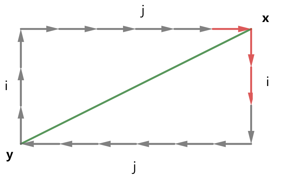
(a) $\Delta_{i}\neq 0$ and $\Delta_{j}\neq 0$, where $1\leq i<j\leq d$.

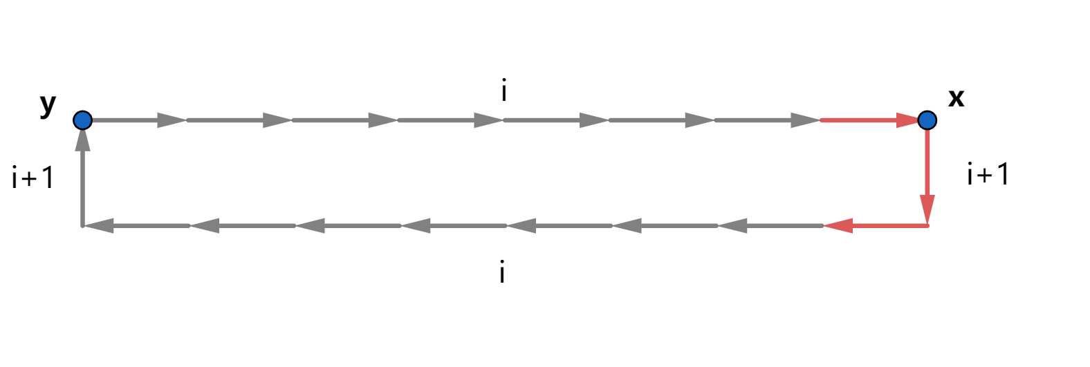
(b) $\Delta_{i}\neq 0$ for some $i<d$. $\Delta_{j}=0$ for all $j\neq i$.

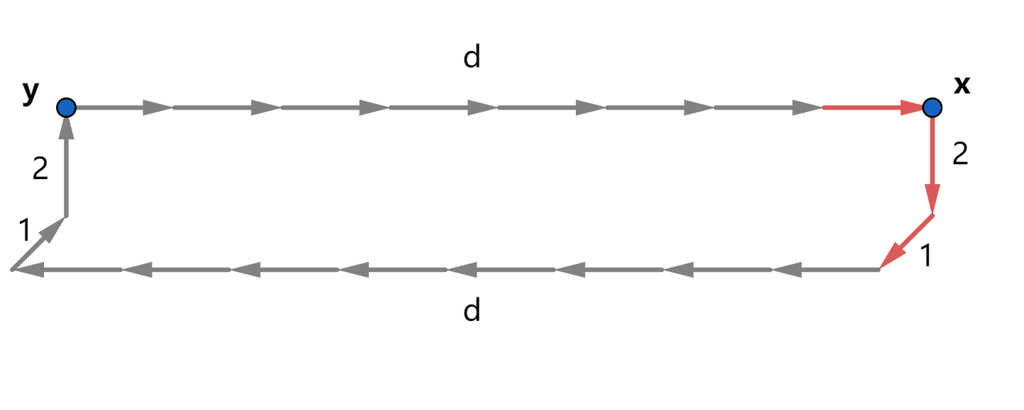
(c) $\Delta_{d}\neq 0$. $\Delta_{j}=0$ for all $j\neq d$

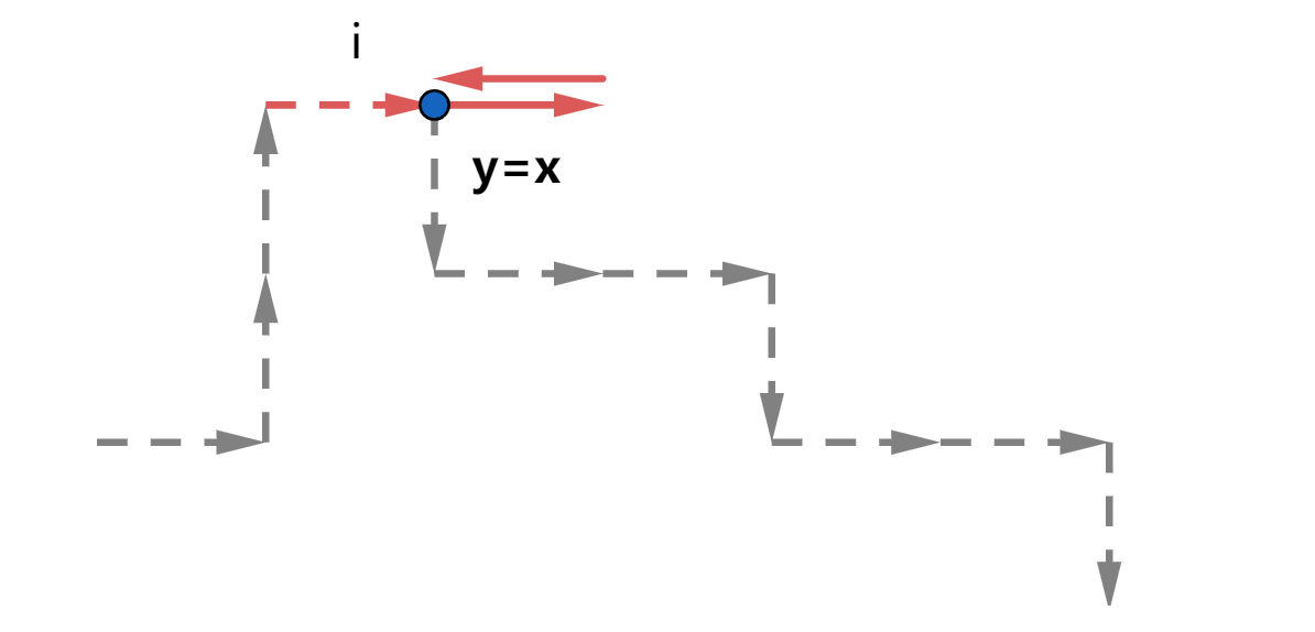
(d) $\boldsymbol{\Delta}=\boldsymbol{0}$

Figure 4.1: The loops $\beta(\boldsymbol{x},\boldsymbol{y})$. A solid short arrow represents a single step of the loop. A number $i$ beside the arrows indicates that this step moves in the $i$-th coordinate. To emphasize the local picture at $\boldsymbol{x}$ for each type, we highlight specific regions with red color. The local structure at $x$ plays a critical role in the proof of Proposition 4.1.

If the type of the vector $\boldsymbol{\Delta}=\boldsymbol{y}-\boldsymbol{x}$ is (a), we construct $\beta=\beta(\boldsymbol{x},\boldsymbol{y})$ as follows. We refer readers to Figure 4.11(a) for reference.

• Let $\beta(0)=\boldsymbol{y}$.

• $\boldsymbol{y}\to\boldsymbol{x}$: For the $k$-th step, if the path $\beta$ has not visited $\boldsymbol{x}$ in the first $(k-1)$ steps, let $i$ be the minimal index such that $\beta(k-1)_{i}\neq x_{i}$, and let the $k$-th step $\beta(k)-\beta(k-1)=e_{i}\cdot\operatorname{sgn}(\Delta_{i})$.

• $\boldsymbol{x}\to\boldsymbol{y}$: For the $k$-th step, if the path $\beta$ has visited $\boldsymbol{x}$ in the first $(k-1)$ steps and $\beta(k-1)\neq\boldsymbol{y}$, let $i$ be the minimum index such that $\beta(k)_{i}\neq y_{i}$, and let the $k$-th step $\beta(k)-\beta(k-1)=-e_{i}\cdot\operatorname{sgn}(\Delta_{i})$. If $\beta(k)=\boldsymbol{y}$ for some $k>0$, we end the path here.

Since $d_{1}(\beta(k+1),\boldsymbol{x})=d_{1}(\beta(k),\boldsymbol{x})-1$ before the path visits $\boldsymbol{x}$ and $d_{1}(\beta(k+1),\boldsymbol{y})=d_{1}(\beta(k),\boldsymbol{y})-1$ after the path visits $\boldsymbol{x}$, the path $\beta$ is a loop connecting $\boldsymbol{y}$ and $\boldsymbol{x}$.

If the type of the vector $\boldsymbol{\Delta}=\boldsymbol{y}-\boldsymbol{x}$ is (b), suppose that $\Delta_{i}\neq 0$, where $1\leq i\leq d-1$. We construct $\beta=\beta(\boldsymbol{x},\boldsymbol{y})$ as follows. We refer readers to Figure 4.11(b) for reference.

• Let $\beta(0)=\boldsymbol{y}$.

• $\boldsymbol{y}\to\boldsymbol{x}$: Let the path $\beta$ move in the direction of $e_{i}\cdot\operatorname{sgn}(\Delta_{i})$ for $|\Delta_{i}|$ steps, and the path $\beta$ visits $\boldsymbol{x}$.

• $\boldsymbol{x}\to\boldsymbol{y}$: First, let the path $\beta$ move in the direction of $e_{i+1}$ for one step. Next, let the path $\beta$ move in the direction of $-e_{i}\cdot\operatorname{sgn}(\Delta_{i})$ for $|\Delta_{i}|$ steps. Finally, let the path $\beta$ move in the direction of $-e_{i+1}$ for one step.

If the type of the vector $\boldsymbol{\Delta}=\boldsymbol{y}-\boldsymbol{x}$ is (c), we construct $\beta=\beta(\boldsymbol{x},\boldsymbol{y})$ as follows. We refer readers to Figure 4.11(c) for reference.

• Let $\beta(0)=\boldsymbol{y}$.

• $\boldsymbol{y}\to\boldsymbol{x}$: Let the path $\beta$ move in the direction of $e_{d}\cdot\operatorname{sgn}(\Delta_{d})$ for $|\Delta_{d}|$ steps, and the path $\beta$ visits $\boldsymbol{x}$.

• $\boldsymbol{x}\to\boldsymbol{y}$: First, let the path $\beta$ move in the direction of $e_{2}$ for one step and then move in the direction of $e_{1}$ for one step. Next, let the path $\beta$ move in the direction of $-e_{d}\cdot\operatorname{sgn}(\Delta_{d})$ for $|\Delta_{d}|$ steps. Finally, let the path $\beta$ move in the direction of $-e_{1}$ for one step and then move in the direction of $-e_{2}$ for one step.

If the type of the vector $\boldsymbol{\Delta}=\boldsymbol{y}-\boldsymbol{x}$ is (d), we have $\boldsymbol{x}=\boldsymbol{y}$. We let $\beta_{i}(\boldsymbol{x})=(\boldsymbol{x},\boldsymbol{x}+e_{i},\boldsymbol{x})$ and choose the loop to be inserted from $\beta_{i}$, $1\leq i\leq d$ according to the path; see the second line of (4.8). We refer readers to Figure 4.11(d) for reference.

Remark.

1. When the type of $\boldsymbol{\Delta}$ is (b) or (c), we introduce extra steps ($\pm e_{i+1}$ for type (b) and $\pm e_{1},\pm e_{2}$ for type (c)) to ensure that the loop $\beta(\boldsymbol{x},\boldsymbol{y})$ is non-self-intersecting, except at the starting point. Furthermore, these extra steps allow us to deduce the type of $\boldsymbol{x}$ from $\widetilde{\omega}$, see Lemma 4.15.

2. When the type of $\boldsymbol{\Delta}$ is (d), loops in the form of $\beta_{i}(\boldsymbol{x})$ are inserted to ensure that the path after loop insertion does not change direction at $\boldsymbol{x}$ when first hitting $\boldsymbol{x}$. This construction enables us to deduce the type of $\boldsymbol{x}$ from $\widetilde{\omega}$; see Lemmas 4.15 and 4.16.

We now turn to the construction of the second kind of loops $\beta^{\mathrm{Tree}}(\mathsf{C},\boldsymbol{x})$, where $\boldsymbol{x}\in\mathsf{C}$ and $\mathsf{C}$ is a subset of $\mathbb{T}_{N}$ with a connected auxiliary graph $G(\mathsf{C})$. The construction proceeds as follows. First, we find an auxiliary loop $\beta^{\operatorname{Tree},\,\mathrm{Aux}}(\mathsf{C},\boldsymbol{x})$ on the auxiliary graph of $\mathsf{C}$, which visits each vertex at least once. Then, we connect the vertices in $\mathsf{C}$ on $\mathbb{T}_{N}$ according to the loop $\beta^{\operatorname{Tree},\,\mathrm{Aux}}(\mathsf{C},\boldsymbol{x})$. We refer readers to Figure 4.2 for reference.

We begin by introducing $\mathsf{Path}(\boldsymbol{y},\boldsymbol{x})$ to convert one step on the auxiliary graph into part of a path on $\mathbb{T}_{N}$.

Definition 4.2.

For two distinct vertices $\boldsymbol{x}\neq\boldsymbol{y}\in\mathbb{T}_{N}$, we define $\mathsf{Path}(\boldsymbol{y},\boldsymbol{x})$ as the $\boldsymbol{y}\to\boldsymbol{x}$ part in the construction of loop $\beta(\boldsymbol{x},\boldsymbol{y})$ when the type of $\boldsymbol{\Delta}=\boldsymbol{y}-\boldsymbol{x}$ is (a), (b) or (c).

In fact, in the definition above one may also choose some other shortest path connecting $\boldsymbol{x}$ and $\boldsymbol{y}$ using another a priori fixed rule that ensures that the loop $\beta^{\operatorname{Tree}}(\mathsf{C},\boldsymbol{x})$ is completely determined by the component $\mathsf{C}$ and root $\boldsymbol{x}$; see the proof of Lemma 4.10. Note that $\mathsf{Path}(\boldsymbol{y},\boldsymbol{x})$ is a non-self-intersecting path connecting $\boldsymbol{y}$ and $\boldsymbol{x}$, with a length no greater than $d|\boldsymbol{x}-\boldsymbol{y}|_{\infty}$, and each vertex $\boldsymbol{z}$ in the path satisfies $|\boldsymbol{z}-\boldsymbol{x}|_{\infty}\leq|\boldsymbol{y}-\boldsymbol{x}|_{\infty}$.

We now define the loop $\beta^{\mathrm{Tree}}(\mathsf{C},\boldsymbol{x})$ by first constructing the auxiliary loop $\beta^{\operatorname{Tree},\,\mathrm{Aux}}(\mathsf{C},\boldsymbol{x})$, and then replacing each step $\boldsymbol{y}\to\boldsymbol{z}$ in $\beta^{\operatorname{Tree},\,\mathrm{Aux}}(\mathsf{C},\boldsymbol{x})$ with $\mathsf{Path}(\boldsymbol{y},\boldsymbol{z})$ to obtain a loop on $\mathbb{T}_{N}$. To construct the auxiliary loop $\beta^{\operatorname{Tree},\,\mathrm{Aux}}(\mathsf{C},\boldsymbol{x})$, we perform a depth-first-search (DFS) algorithm to explore the graph $G(\mathsf{C})$ and record the order each vertex is visited. We refer readers to Figures 4.22(b), 4.22(c) and 4.22(d) for reference.

Definition 4.3.

For each $\mathsf{C}\subset\mathbb{T}_{N}$ and $\boldsymbol{x}\in\mathsf{C}$, we apply DFS to generate a spanning tree $\operatorname{Tree}(\mathsf{C})$ rooted at $\boldsymbol{x}$. The sequence of vertices visited during the exploration forms a loop on the graph $G(\mathsf{C})$, which is denoted by $\beta^{\operatorname{Tree},\,\mathrm{Aux}}(\mathsf{C},\boldsymbol{x})$. We now write $\beta^{\mathrm{Tree},\mathrm{Aux}}(\mathsf{C},\boldsymbol{x})=(\boldsymbol{z}_{0},\boldsymbol{z}_{1},\ldots,\boldsymbol{z}_{L})$ and concatenate the paths $\mathsf{Path}(\boldsymbol{z}_{i},\boldsymbol{z}_{i+1})$, $0\leq i\leq L-1$ in sequence to obtain a loop on the graph $\mathbb{T}_{N}$, which is denoted by $\beta^{\mathrm{Tree}}(\mathsf{C},\boldsymbol{x})$.

It is elementary that the loop $\beta^{\mathrm{Tree}}(\mathsf{C},\boldsymbol{x})$ is completely determined by the subset $\mathsf{C}$ and the vertex $\boldsymbol{x}$.

(a) Vertices in the set $\mathsf{C}$. The side-length of the cubes is $l_{N}$. Vertices are labeled with black numbers.

(b) Auxiliary graph $\mathsf{C}$ and $\mathsf{Tree}(\mathsf{C})$. Edges of $\mathsf{Tree}(\mathsf{C})$ are highlighted in red.

(c) Loop $\beta^{\mathrm{Tree},\mathrm{Aux}}(\mathsf{C})$. Steps of loop $\beta^{\mathrm{Tree},\mathrm{Aux}}(\mathsf{C})$ are represented by the blue arrows.

(d) Loop $\beta^{\mathrm{Tree}}(\mathsf{C})$. Steps of $\beta^{\mathrm{Tree}}(\mathsf{C})$ are represented by the blue arrows. The blue arrows next to the number $k$ correspond to the $k$-th step of loop $\beta^{\mathrm{Tree},\mathrm{Aux}}(\mathsf{C})$.

Figure 4.2: Construction of loop $\beta^{\mathrm{Tree}}(\mathsf{C},\boldsymbol{x})$.

We conclude this subsection by stating some key properties of loops $\beta(\boldsymbol{x},\boldsymbol{y})$ and $\beta^{\mathrm{Tree}}(\mathsf{C},\boldsymbol{x})$, which are used in the proof of Proposition 4.1. We omit their proofs as they can be easily verified from the definition.

The first property provides upper bounds for the length of the loops constructed above. Recall that we define $L(\omega)$ as the length of the path $\omega$; see below (1.2) for reference.

Lemma 4.4.

1. For two vertices $\boldsymbol{x},\boldsymbol{y}\in\mathbb{T}_{N}$, we have

   (4.4) $$L(\beta(\boldsymbol{x},\boldsymbol{y}))\leq 2d\cdot(d_{\infty}(\boldsymbol{x},\boldsymbol{y})+2).$$

2. For each $\mathsf{C}\subset\mathbb{T}_{N}$ and $\boldsymbol{x}\in\mathsf{C}$, we have

   (4.5) $$L(\beta^{\mathrm{Tree}}(\mathsf{C},\boldsymbol{x}))\leq 6dl_{N}(|\mathsf{C}|-1).$$

The second key property is that the part of the loop $\beta(\boldsymbol{x},\boldsymbol{y})$ before hitting $\boldsymbol{x}$ and the part of the loop $\beta(\boldsymbol{x},\boldsymbol{y})$ after hitting $\boldsymbol{x}$ are disjoint. This property allows us to deduce $\beta(\boldsymbol{x},\boldsymbol{y})$ from $\widetilde{\omega}\in\Psi(\omega)$, enabling the recovery of the path $\omega$ from $\widetilde{\omega}$.

Lemma 4.5.

For all distinct $\boldsymbol{x}\neq\boldsymbol{y}\in\mathbb{T}_{N}$, the loop $\beta=\beta(\boldsymbol{x},\boldsymbol{y})$ satisfies

(4.6) $$\beta[1,H_{\boldsymbol{x}}-1]\cap\beta[H_{\boldsymbol{x}}+1,L(\beta)-1]=\emptyset,$$

where $H_{\boldsymbol{x}}$ is the time when the loop $\beta$ first hits vertex $\boldsymbol{x}$.

4.2 Loop insertion

In this subsection, we will construct the mapping $\Psi$ in the statement of Proposition 4.1 by first inserting loops $\beta(\boldsymbol{x},\boldsymbol{y})$ and $\beta^{\mathrm{Tree}}(\mathsf{C},\boldsymbol{x})$ into the path $\omega$ (at Stage 3 of the strategy), and then allowing the path to roam freely (at Stage 4). To describe the exact time (and location) to insert these loops, we introduce the hitting time of the path $\omega$ for a vertex $\boldsymbol{z}\in\mathbb{T}_{N}$ as follows:

(4.7) $$H_{\lambda}(\omega,\boldsymbol{z})=\inf\{k\geq\lambda t_{\operatorname{cov}}\,:\,\omega(k)=\boldsymbol{z}\},$$

which is the first time that the path $\omega$ hits the vertex $\boldsymbol{z}$ after time $\lambda t_{\operatorname{cov}}$.

We are ready to define the mapping $\Psi$. From now on in this subsection, we fix the path $\omega\in\mathcal{A}$, where $\mathcal{A}$ is an $(\boldsymbol{F},\varepsilon,M_{0})$-good path collection; see Definition 3.2 for the definition of $(\boldsymbol{F},\varepsilon,M_{0})$-good path collections.

The first step is to insert loops of the form $\beta_{\boldsymbol{x}}$ defined below to connect the vertices in $\mathcal{R}(\mathcal{L}^{\beta_{N}}_{\boldsymbol{F}}(\omega))$ to the path $\omega$. Recall the definition of $\mathsf{Near}(\cdot,\cdot)$ and the types of $\boldsymbol{x}$ at the beginning of Section 4.1.

Definition 4.6.

For all $\omega\in\mathcal{A}$ and $\boldsymbol{x}\in\mathcal{R}(\mathcal{L}_{\boldsymbol{F}}^{\beta_{N}}(\omega))$, we define

(4.8) $$\beta_{\boldsymbol{x}}=\beta_{\boldsymbol{x}}(\omega)=\begin{cases}\beta(\boldsymbol{x},\mathsf{Near}(\omega,\boldsymbol{x}))&\text{if $\boldsymbol{x}\neq\mathsf{Near}(\omega,\boldsymbol{x})$},\\ \beta_{i}(\boldsymbol{x})&\text{if $\boldsymbol{x}=\mathsf{Near}(\omega,\boldsymbol{x})$ and $\mathsf{Dir}(\omega,H_{\beta_{N}}(\omega,\mathsf{Near}(\omega,\boldsymbol{x}))-1)=i$},\end{cases}$$

where $\mathsf{Dir}(\omega,k)=i$ if $\omega(k+1)-\omega(k)=\pm e_{i}$ for a path $\omega$ and $k\geq 0$. Moreover, we define

(4.9) $$B(\omega)=\{\beta_{\boldsymbol{x}}(\omega)\,:\,\boldsymbol{x}\in\mathcal{R}(\mathcal{L}^{\beta_{N}}_{\boldsymbol{F}}(\omega))\}$$

as the collection of loops to be inserted in the first step.

For each $\boldsymbol{x}\in\mathcal{R}(\mathcal{L}^{\beta_{N}}_{\boldsymbol{F}}(\omega))$, the loop $\beta_{\boldsymbol{x}}(\omega)$ is inserted one-by-one to connect $\boldsymbol{x}$ to the path $\omega$ at time $H_{\beta_{N}}(\omega,\mathsf{Near}(\omega,\boldsymbol{x}))$. It remains to determine the order of insertion. We now claim that the mapping $\mathsf{Near}(\omega,\cdot)\mid_{\mathcal{R}(\mathcal{L}^{\beta_{N}}_{\boldsymbol{F}}(\omega))}$ is injective, which ensures that $H_{\beta_{N}}(\omega,\mathsf{Near}(\omega,\boldsymbol{x}))\neq H_{\beta_{N}}(\omega,\mathsf{Near}(\omega,\boldsymbol{x}^{\prime}))$ for all $\boldsymbol{x}\neq\boldsymbol{x}^{\prime}\in\mathcal{R}(\mathcal{L}^{\beta_{N}}_{\boldsymbol{F}}(\omega))$. Hence, we can label the elements of $\mathcal{R}(\mathcal{L}_{\boldsymbol{F}}^{\beta_{N}}(\omega))$ as $\boldsymbol{x}_{1},\boldsymbol{x}_{2},\ldots\boldsymbol{x}_{n}$, where

(4.10) $$n=|\mathcal{R}(\mathcal{L}_{\boldsymbol{F}}^{\beta_{N}}(\omega))|,$$

in such a way that $H_{\beta_{N}}(\omega,\mathsf{Near}(\omega,\boldsymbol{x}_{l}))$ is strictly increasing with respect to $l$. For simplicity, we let $\beta^{(l)}=\beta^{(l)}(\omega)=\beta_{\boldsymbol{x}_{l}}(\omega)$, which gives an order on $B(\omega)$. Furthermore, we denote $H_{\beta_{N}}(\omega,\mathsf{Near}(\omega,\boldsymbol{x}_{l}))$ by $H_{l}(\omega)$ for the remainder of this section.

We now recursively insert the loops in $B(\omega)$ to connect the vertices in $\mathcal{R}(\mathcal{L}^{\beta_{N}}_{\boldsymbol{F}}(\omega))$ to the path $\omega$. Recall again the definition of $\Omega_{k}$ below (1.2). For a path $\omega\in\Omega_{L_{1}}$, a loop $\beta\in\Omega_{L_{2}}$ and $0\leq k\leq L_{1}$ such that $\omega(k)=\beta(0)=\beta(L_{2})$, we define the insertion map $\mathsf{Ins}(\omega,\beta,k)\in\Omega_{L_{1}+L_{2}}$ whose output is the new path with $\beta$ inserted into $\omega$ at time $k$.

We now set $\omega^{(0)}=\omega$ and $S^{(0)}(\omega)=0$. Using the mapping $\mathsf{Ins}$, we recursively define the result and total duration after $l$-th insertion, denoted by $\omega^{(l)}$ and $S^{(l)}$ resp. for $1\leq l\leq n$ as follows:

(4.11) $$\omega^{(l)}=\mathsf{Ins}(\omega^{(l-1)},\beta^{(l)},H_{l}(\omega)+S^{(l-1)}(\omega)),\quad S^{(l)}(\omega)=S^{(l-1)}(\omega)+L(\beta^{(l)}).$$

We now turn to the second step at Stage 3, which involves inserting loops in the form of $\beta^{\mathrm{Tree}}(\mathsf{C},\boldsymbol{x})$ to cover the remaining late points $\mathcal{L}_{\boldsymbol{F}}^{\beta_{N}}(\omega)\setminus\mathcal{R}(\mathcal{L}_{\boldsymbol{F}}^{\beta_{N}}(\omega))$.

Recall that $\mathcal{C}(\mathcal{L}_{\boldsymbol{F}}^{\beta_{N}}(\omega))$ represents the collection of connected components of $G(\mathcal{L}_{\boldsymbol{F}}^{\beta_{N}}(\omega))$. There exists a natural bijection $\boldsymbol{x}\mapsto\mathsf{C}_{\boldsymbol{x}}$ between $\mathcal{R}(\mathcal{L}_{\boldsymbol{F}}^{\beta_{N}}(\omega))$ and $\mathcal{C}(\mathcal{L}_{\boldsymbol{F}}^{\beta_{N}}(\omega))$ such that $\boldsymbol{x}\in\mathsf{C}_{\boldsymbol{x}}$.

Definition 4.7.

For each $\omega\in\mathcal{A}$ and $\boldsymbol{x}\in\mathcal{R}(\mathcal{L}_{\boldsymbol{F}}^{\beta_{N}}(\omega))$, we define the collection of loops to be inserted in the second step as follows:

(4.12) $$B^{\operatorname{Tree}}(\omega)=\big{\{}\beta^{\operatorname{Tree}}(\mathsf{C}_{\boldsymbol{x}},\boldsymbol{x})\,:\,\boldsymbol{x}\in\mathcal{R}(\mathcal{L}_{\boldsymbol{F}}^{\beta_{N}}(\omega))\big{\}}.$$

For clarity, we denote $\beta^{(l),\text{Tree}}=\beta^{\mathrm{Tree}}(\mathsf{C}_{\boldsymbol{x}_{l}},\boldsymbol{x}_{l})$, which provides an order on $B^{\operatorname{Tree}}(\omega)$. For simplicity, let $H_{l}(\omega^{(n)})=H_{\beta_{N}}(\omega^{(n)},\boldsymbol{x}_{l})$.

We now recursively insert the loops in $B^{\operatorname{Tree}}(\omega)$. We initialize by setting $S^{(0),\text{Tree}}(\omega)=0$. For each $1\leq l\leq n$, write

(4.13) $$\begin{split}\omega^{(n+l)}&=\mathsf{Ins}(\omega^{(n+l-1)},\beta^{(l),\text{Tree}},H_{l}(\omega^{(n)})+S^{(l-1),\text{Tree}}(\omega));\\ S^{(l),\text{Tree}}(\omega)&=S^{(l-1),\text{Tree}}(\omega)+L(\beta^{(l),\text{Tree}})\end{split}$$

for the result and total duration after $l$-th insertion, respectively.

The final step of constructing $\Psi$ involves converting the path $\omega^{(2n)}$ into paths of length $T_{4}$, corresponding to Stage 4. By estimating the total length of the loops inserted, we can show that $L(\omega^{(2n)})\leq T_{4}$ for all $\omega\in\mathcal{A}$; see Lemma 4.9 below. This ensures that the path $\omega^{(2n)}$ can continue to roam freely after the time $L(\omega^{(2n)})$ until it reaches the total length $T_{4}$. We collect all such extended paths into the set defined as $\Psi(\omega)$.

Definition 4.8.

For all $\omega\in\mathcal{A}$, we let

(4.14) $$\Psi(\omega)=\Big{\{}\widetilde{\omega}\in\Omega_{T_{4}}:\widetilde{\omega}=\omega^{(2n)}|_{L(\omega^{(2n)})}\Big{\}}.$$

The construction of the mapping $\Psi$ is now complete.

4.3 Proof of Proposition 4.1

The claim (4.1a) is a direct consequence of the construction of $\Psi$ and (3.12a). We hence omit the proof.

We now proceed to the proof of (4.1b). The key to the proof lies in establishing an upper bound for $L(\omega^{(2n)})$, which is provided in Lemma 4.9.

Lemma 4.9.

For all $\omega\in\mathcal{A}$, where $\mathcal{A}$ is an $(\boldsymbol{F},\varepsilon,M_{0})$-good path collection, we have

(4.15) $$L(\omega^{(2n)})\leq T_{3}+J(\boldsymbol{F},M_{0}),$$

where $J(\boldsymbol{F},M_{0})$ is defined in (3.13). In particular, by (3.14), we have $L(\omega^{(2n)})\leq T_{4}$.

Proof of (4.1b) assuming Lemma 4.9.

From the definition of $\Psi$ in (4.14), we know that

(4.16) $$|\Psi(\omega)|=(2d)^{T_{4}-L(\omega^{(2n)})}.$$

Combining this with (4.15) gives (4.1b). ∎

We now prove Lemma 4.9 by estimating the total length of the loops inserted at Stage 3.

Proof of Lemma 4.9.

By the definition of $\Psi$, we have

(4.17) $$L(\omega^{(2n)})=T_{3}+S^{(n)}(\omega)+S^{(n),\text{Tree}}(\omega).$$

Thus, it suffices to bound $S^{(n)}(\omega)$ and $S^{(n),\text{Tree}}(\omega)$ separately.

For $S^{(n)}(\omega)$, we recall the definition of $\boldsymbol{r}_{x}(\omega)$ (see (3.8)) and $\mathsf{Near}(\cdot,\cdot)$ (see the beginning of Section 4.1), and obtain by (4.4)

(4.18) $$S^{(n)}(\omega)=\sum_{\boldsymbol{x}\in\mathcal{R}(\mathcal{L}_{\boldsymbol{F}}^{\beta_{N}}(\omega))}L(\beta(\boldsymbol{x},\mathsf{Near}(\omega,\boldsymbol{x})))\leq\sum_{\boldsymbol{x}\in\mathcal{R}(\mathcal{L}_{\boldsymbol{F}}^{\beta_{N}}(\omega))}2d(\boldsymbol{r}_{\boldsymbol{x}}(\omega)+2).$$

For $S^{(n),\text{Tree}}(\omega)$, we recall $n=|\mathcal{R}(\mathcal{L}_{\boldsymbol{F}}^{\beta_{N}}(\omega))|$ (see (4.10)) and obtain by (4.5)

(4.19) $$S^{(n),\operatorname{Tree}}(\omega)=\sum_{l=1}^{n}L(\beta^{\operatorname{Tree}}(\mathsf{C}_{l},\boldsymbol{x}_{l}))\leq\sum_{\mathsf{C}\in\mathcal{C}(\mathcal{L}_{\boldsymbol{F}}^{\beta_{N}}(\omega))}6dl_{N}(|\mathsf{C}|-1)=6dl_{N}(|\mathcal{L}_{\boldsymbol{F}}^{\beta_{N}}(\omega)|-|\mathcal{R}(\mathcal{L}_{\boldsymbol{F}}^{\beta_{N}}(\omega))|),$$

where the last equation follows from $|\mathcal{C}(\mathcal{L}_{\boldsymbol{F}}^{\beta_{N}}(\omega))|=n$ and the fact that $\mathcal{C}(\mathcal{L}_{\boldsymbol{F}}^{\beta_{N}}(\omega))$ is a partition of $\mathcal{L}_{\boldsymbol{F}}^{\beta_{N}}(\omega)$. Hence, the total length of the loops inserted at Stage 3 is

(4.20) $$S^{(n)}(\omega)+S^{(n),\text{Tree}}(\omega)\overset{\eqref{eq: upper bound for total length in STEP 1}}{} {\underset{\eqref{eq: upper bound for total length in STEP 2}}{\leq}}\sum_{\boldsymbol{x}\in\mathcal{R}(\mathcal{L}_{\boldsymbol{F}}^{\beta_{N}}(\omega))}2d(\boldsymbol{r}_{\boldsymbol{x}}(\omega)+2)+6dl_{n}(|\mathcal{L}_{\boldsymbol{F}}^{\beta_{N}}(\omega)|-|\mathcal{R}(\mathcal{L}_{\boldsymbol{F}}^{\beta_{N}}(\omega))|)$$

$$\overset{\eqref{no too much cost for extra loops}}{} {\underset{\eqref{cost of inserting loops}}{\leq}}J(\boldsymbol{F},M_{0}).$$

Note that (3.12c) holds here because $\omega$ is a path in the $(\boldsymbol{F},\varepsilon,M_{0})$-good path collection $\mathcal{A}$. Combining this with (4.17) gives (4.15). ∎

We now turn to the proof of (4.1c). Suppose that $\widetilde{\omega}\in\Psi(\mathcal{A})$, where $\Psi(\mathcal{A})\overset{\text{def.}}{=}\bigcup_{\omega\in\mathcal{A}}\Psi(\omega)$. Intuitively, if all loops and their insertion locations can be uniquely identified from $\widetilde{\omega}$, we can remove these loops to recover the original path. After deleting all such loops from $\widetilde{\omega}$, the first $T_{3}$ steps of the resulting path gives $\omega$.

For two paths $\omega,\widehat{\omega}\in\Omega$, we say that $\widehat{\omega}$ is an extension of $\omega$ if $L(\widehat{\omega})\geq L(\omega)$ and $\widehat{\omega}=\omega\mid_{L(\omega)}$. It is obvious that if $\widehat{\omega}$ is an extension of $\omega$ and $L(\omega)\geq\lambda t_{\operatorname{cov}}$, then $H_{\lambda}(\omega,\boldsymbol{x})=H_{\lambda}(\widehat{\omega},\boldsymbol{x})$ for all $\boldsymbol{x}\in\omega[\lambda t_{\operatorname{cov}},L(\omega)]$. Given a path $\omega\in\Omega$ and indices $0\leq k_{1}<k_{2}\leq L(\omega)$ such that $\omega(k_{1})=\omega(k_{2})$, we define $\mathsf{Del}(\omega,k_{1},k_{2})\in\Omega_{L(\omega)-k_{2}+k_{1}}$ as the result of removing the loop $\omega(k_{1},\ldots,k_{2})$ from $\omega$.

We now recover $\omega$ from $\widetilde{\omega}$. We first show that we can recover the path $\omega^{(n)}$ from $\widetilde{\omega}$ by deleting the loops inserted in the second step. Then, we show that $\omega$ can be recovered from $\omega^{(n)}$.

In the following lemma, we show that an extension of path $\omega^{(n)}$ can be obtained by identifying the set $B^{\operatorname{Tree}}(\omega)$ and deleting the loops it contains.

Lemma 4.10.

For any $\widetilde{\omega}\in\Psi(\mathcal{A})$, where $\mathcal{A}$ is an $(\boldsymbol{F},\varepsilon,M_{0})$-good path collection, there exists a path $\overline{\omega}$ such that for any $\omega\in\mathcal{A}$ satisfying $\widetilde{\omega}\in\Psi(\omega)$, the path $\overline{\omega}$ is an extension of $\omega^{(n)}$.

For clarity in the following proof, we say that a mapping $\mathsf{Obj}(\cdot)$ with domain $\mathcal{A}$ (e.g. $B^{\operatorname{Tree}}(\cdot)$, $\mathcal{L}_{\boldsymbol{F}}^{\beta_{N}}(\cdot)$, etc.) is determined by $\widetilde{\omega}$ if $\mathsf{Obj}(\omega)$ remains the same for all $\omega\in\mathcal{A}$ such that $\widetilde{\omega}\in\Psi(\omega)$. With slight abuse of notation, we also say that $\mathsf{Obj}(\omega)$ is determined by $\widetilde{\omega}$ if it is presupposed that $\widetilde{\omega}\in\Psi(\omega)$ and the mapping $\mathsf{Obj}(\cdot)$ is determined by $\widetilde{\omega}$.

Proof.

Let $\widetilde{\omega}\in\Psi(\mathcal{A})$, and fix $\omega\in\mathcal{A}$ such that $\widetilde{\omega}\in\Psi(\omega)$. We aim to establish that the set $B^{\operatorname{Tree}}(\omega)$ is determined by $\widetilde{\omega}$. Since the insertion of loops occurs only after $T_{2}$ (by the definition of $\Psi$), it follows that $\widetilde{\omega}=\omega\mid_{T_{2}}$. Hence, $\mathcal{L}_{\boldsymbol{F}}^{\beta_{N}}(\widetilde{\omega})=\mathcal{L}_{\boldsymbol{F}}^{\beta_{N}}(\omega)$. The definition of $B^{\operatorname{Tree}}(\omega)$ depends solely on the set $\mathcal{L}_{\boldsymbol{F}}^{\beta_{N}}(\omega)$, and thus $B^{\operatorname{Tree}}(\omega)$ is determined by $\widetilde{\omega}$.

Note $n$ (see (4.10) for definition) is also determined by $\widetilde{\omega}$. To delete the loops in $B^{\operatorname{Tree}}(\omega)$ via the mapping $\mathsf{Del}$, it is necessary to demonstrate that $H_{l}(\omega^{(n)})+S^{(l-1),\text{Tree}}(\omega)$, the times to insert loops into the original path, is determined by $\widetilde{\omega}$. Recall that we have written the set $\mathcal{R}(\mathcal{L}_{\boldsymbol{F}}^{\beta_{N}}(\omega))$ as $\boldsymbol{x}_{1},\boldsymbol{x}_{2},\ldots,\boldsymbol{x}_{n}$. Although the representation may depend on $\omega$, the set $\mathcal{L}_{\boldsymbol{F}}^{\beta_{N}}(\omega)$ is determined by $\widetilde{\omega}$. Note that $\boldsymbol{x}_{l}\notin\beta^{(l^{\prime}),\mathrm{Tree}}$ and $\boldsymbol{x}_{l}\notin\beta^{(l^{\prime})}$ when $l^{\prime}\neq l$, so $\omega$ visits the vertices $\mathsf{Near}(\omega,\boldsymbol{x}_{l})$ after time $T_{2}$ in the same sequence as $\widetilde{\omega}$ visits vertices $\boldsymbol{x}_{l}$ after time $T_{2}$. This ensures that the expression $\boldsymbol{x}_{1},\boldsymbol{x}_{2},\ldots,\boldsymbol{x}_{n}$ is determined by $\widetilde{\omega}$. Furthermore, by the definition of $\omega^{(n+l)}$ and $S^{(l)}$, we obtain

(4.21) $$H_{\beta_{N}}(\widetilde{\omega},\boldsymbol{x}_{l})=H_{\beta_{N}}(\omega^{(n+l^{\prime})},\boldsymbol{x}_{l})=H_{l}(\omega^{(n)})+S^{(l-1),\text{Tree}}(\omega)\,\,\,\,\mbox{ for all $1\leq l\leq l^{\prime}\leq n$},$$

which implies that $H_{l}(\omega^{(n)})+S^{(l-1),\text{Tree}}(\omega)$ is determined by $\widetilde{\omega}$.

Consider the following deletion process. We start with the loop $\widetilde{\omega}^{(2n)}=\widetilde{\omega}$ and define recursively

(4.22) $$\widetilde{\omega}^{(n+l-1)}=\mathsf{Del}(\widetilde{\omega}^{(n+l)},H_{l}(\omega^{(n)})+S^{(l-1),\text{Tree}}(\omega),H_{l}(\omega^{(n)})+S^{(l-1),\text{Tree}}(\omega)+L(\beta^{\operatorname{Tree},(l)})),$$

for all $1\leq l\leq n$. By induction, we can derive that $\mathsf{Del}$ can be applied as shown in (4.22) and $\widetilde{\omega}^{(n+l)}$ is an extension of $\omega^{(n+l)}$ for all $0\leq l\leq n$. Since the deletion process is determined by $\widetilde{\omega}$ from the discussion above, the path $\widehat{\omega}=\widetilde{\omega}^{(n)}$ is also determined by $\widetilde{\omega}$. This finishes the proof of Lemma 4.10. ∎

To recover $\omega$ from $\widetilde{\omega}^{(n)}$, we show that it is possible to recover $\omega$ from any extension of $\omega^{(n)}$. Define $\overline{\Psi}(\omega)$ as the collection of all extensions of $\omega^{(n)}$, and let $\overline{\Psi}(\mathcal{A})\overset{\text{def.}}{=}\bigcup_{\omega\in\mathcal{A}}\overline{\Psi}(\omega)$. We state the following proposition:

Proposition 4.11.

Suppose that $\overline{\omega}\in\overline{\Psi}(\mathcal{A})$, where $\mathcal{A}$ is an $(\boldsymbol{F},\varepsilon,M_{0})$-good path collection. There exists a unique path $\omega\in\mathcal{A}$ such that $\overline{\omega}\in\overline{\Psi}(\omega)$.

The proof is deferred to Section 4.4. The central idea of the proof involves identifying the set $B(\omega)$, followed by deletion of the loops.

Proof of (4.1c) assuming Proposition 4.11.

For an $(\boldsymbol{F},\varepsilon,M_{0})$-good path collection $\mathcal{A}$, suppose that there exists $\omega,\omega^{\prime}\in\mathcal{A}$ such that $\Psi(\omega)\cap\Psi(\omega^{\prime})\neq\emptyset$. Then there exists a path $\widetilde{\omega}\in\Psi(\omega)\cap\Psi(\omega^{\prime})$. For simplicity, we let $n=|\mathcal{R}(\mathcal{L}_{\boldsymbol{F}}^{\beta_{N}}(\omega))|$ and $n^{\prime}=|\mathcal{R}(\mathcal{L}_{\boldsymbol{F}}^{\beta_{N}}(\omega^{\prime}))|$. By Lemma 4.10, there exists a path $\overline{\omega}$ such that $\overline{\omega}$ is both an extension of $\omega^{(n)}$ and an extension of $(\omega^{\prime})^{(n^{\prime})}$, which implies $\overline{\omega}\in\overline{\Psi}(\omega)\cap\overline{\Psi}(\omega^{\prime})$. We now apply Proposition 4.11 to the path $\overline{\omega}$ and conclude that $\omega=\omega^{\prime}$. ∎

4.4 Proof of Proposition 4.11

In this subsection, we prove Proposition 4.11. The main approach parallels the proof of Lemma 4.10, but demands more intricate technical arguments. For the remainder of this subsection, we fix $\overline{\omega}\in\overline{\Psi}(\mathcal{A})$. For ease of exposition, we introduce the notion that $\mathsf{Obj}(\omega)$ is determined by $\overline{\omega}$. Note that the meaning of “$\mathsf{Obj}(\omega)$ is determined by $\overline{\omega}$” in this subsection slightly differs from that of “$\mathsf{Obj}(\omega)$ is determined by $\widetilde{\omega}$” in the previous subsection.

Definition 4.12.

For a path $\overline{\omega}\in\overline{\Psi}(\mathcal{A})$ and a mapping $\mathsf{Obj}(\cdot)$ with domain $\mathcal{A}$ (e.g. $\mathcal{L}_{\boldsymbol{F}}^{\beta_{N}}(\cdot)$, $B(\cdot)$ in (4.9), or the mapping that maps $\omega\in\mathcal{A}$ to the loop insertion process described in (4.11) etc.), we say that $\mathsf{Obj}(\cdot)$ is determined by $\overline{\omega}$ if $\mathsf{Obj}(\omega)$ is identical for all $\omega\in\mathcal{A}$ satisfying $\overline{\omega}\in\overline{\Psi}(\omega)$. With slight abuse of notation, we also say that $\mathsf{Obj}(\omega)$ is determined by $\overline{\omega}$ if we assume $\overline{\omega}\in\overline{\Psi}(\omega)$ and the mapping $\mathsf{Obj}(\cdot)$ is determined by $\overline{\omega}$.

Recall that at the beginning of Section 4.2, we have fixed the path $\omega\in\mathcal{A}$ where $\mathcal{A}$ is an $(\boldsymbol{F},\varepsilon,M_{0})$-good path collection. Also recall that $B(\omega)$, defined in Definition 4.6, is the set of loops inserted to construct $\omega^{(n)}$. We begin by showing that the set $B(\omega)$ can be identified.

Lemma 4.13.

For all $\overline{\omega}\in\overline{\Psi}(\mathcal{A})$ and $\omega\in\mathcal{A}$ such that $\overline{\omega}\in\overline{\Psi}(\omega)$, the loop collection $B(\omega)$ is determined by $\overline{\omega}$.

To establish Lemma 4.13, we begin by identifying the late points set $\mathcal{L}_{\boldsymbol{F}}^{\beta_{N}}(\omega)$.

Lemma 4.14.

For all $\overline{\omega}\in\overline{\Psi}(\mathcal{A})$ and $\omega\in\mathcal{A}$ such that $\overline{\omega}\in\overline{\Psi}(\omega)$, the late points set $\mathcal{L}_{\boldsymbol{F}}^{\beta_{N}}(\omega)$ is determined by $\overline{\omega}$. In particular, $\mathcal{R}(\mathcal{L}_{\boldsymbol{F}}^{\beta_{N}}(\omega))$ is also determined by $\overline{\omega}$.

Proof.

Note that the insertion of loops occurs only after $T_{2}$ (by definition of $\Psi$), implying $\omega=\omega^{(n)}\mid_{T_{2}}$. Since $\overline{\omega}$ is an extension of $\omega^{(n)}$, it follows that $\omega=\overline{\omega}\mid_{T_{2}}$. Therefore, $\mathcal{L}_{\boldsymbol{F}}^{\beta_{N}}(\omega)=\mathcal{L}_{\boldsymbol{F}}^{\beta_{N}}(\overline{\omega})$, which implies Lemma 4.14. ∎

After identifying the set $\mathcal{R}(\mathcal{L}_{\boldsymbol{F}}^{\beta_{N}}(\omega))$, we only need to identify $\beta_{\boldsymbol{x}}(\omega)$, the loop associated with each vertex $\boldsymbol{x}\in\mathcal{R}(\mathcal{L}_{\boldsymbol{F}}^{\beta_{N}}(\omega))$. This process will be divided into two steps. First, we identify the type of $\boldsymbol{x}$, as demonstrated in Lemma 4.15. Next, assuming that the type of $\boldsymbol{x}$ is known, we identify $\beta_{\boldsymbol{x}}(\omega)$ in Lemma 4.17.

Recall the definition of the type of $\boldsymbol{x}$, introduced at the beginning of Section 4.1.

Lemma 4.15.

For all $\overline{\omega}\in\overline{\Psi}(\mathcal{A})$ and $\omega\in\mathcal{A}$ such that $\overline{\omega}\in\overline{\Psi}(\omega)$, the type of each vertex $\boldsymbol{x}\in\mathcal{R}(\mathcal{L}_{\boldsymbol{F}}^{\beta_{N}}(\omega))$ is determined by $\overline{\omega}$.

Note that the type of each vertex $\boldsymbol{x}\in\mathcal{R}(\mathcal{L}_{\boldsymbol{F}}^{\beta_{N}}(\omega))$ may depend on the path $\omega$, as $\mathsf{Near}(\omega,\boldsymbol{x})$ is defined in terms of $\omega$. Recall that we have given each vertex in $\mathcal{R}(\mathcal{L}_{\boldsymbol{F}}^{\beta_{N}}(\omega))$ a label $l\in[1,n]$ (possibly depending on $\omega$) above (4.10). To prove Lemma 4.15, we first show that the local structure of $\beta^{(l)}$ near $\boldsymbol{x}_{l}$, where $\boldsymbol{x}_{l}\in\mathcal{R}(\mathcal{L}_{\boldsymbol{F}}^{\beta_{N}}(\omega))$, can be deduced from $\overline{\omega}$. Recall the definition of $\mathsf{Dir}(\omega,k)$ above (4.9).

Lemma 4.16.

Suppose $\omega\in\mathcal{A}$ and $\overline{\omega}\in\overline{\Psi}(\omega)$. For all $\boldsymbol{x}_{l}\in\mathcal{R}(\mathcal{L}_{\boldsymbol{F}}^{\beta_{N}}(\omega))$:

1. If the type of $\boldsymbol{x}_{l}$ is (d), we have

   (4.23) $$\mathsf{Dir}(\overline{\omega},H_{\beta_{N}}(\overline{\omega},\boldsymbol{x}_{l}))=\mathsf{Dir}(\overline{\omega},H_{\beta_{N}}(\overline{\omega},\boldsymbol{x}_{l})-1).$$

2. If the type of $\boldsymbol{x}_{l}$ is not (d), we have

   (4.24) $$\mathsf{Dir}(\overline{\omega},H_{\beta_{N}}(\overline{\omega},\boldsymbol{x}_{l})+i)=\mathsf{Dir}(\beta^{(l)},H_{0}(\beta^{(l)},\boldsymbol{x}_{l})+i),\quad i\in\{0,\pm 1\}.$$

Proof.

Recall $n=|\mathcal{R}(\mathcal{L}_{\boldsymbol{F}}^{\beta_{N}}(\omega))|$ in (4.10) and the definitions of $H_{l}(\omega)$, $S^{(l)}(\omega)$ and $\omega^{(l)}$ in (4.11) for $1\leq l\leq n$. We first show that loops in $B(\omega)$ (see (4.9)) are mutually disjoint. Recall that $d_{\infty}(\boldsymbol{x},\mathsf{Near}(\omega,\boldsymbol{x}))\leq l_{n}$ for each $\boldsymbol{x}\in\mathcal{R}(\mathcal{L}^{\beta_{N}}_{\boldsymbol{F}}(\omega))$ and $d_{\infty}(\boldsymbol{x},\boldsymbol{x}^{\prime})>3l_{N}$ for all $\boldsymbol{x}\neq\boldsymbol{x}^{\prime}\in\mathcal{R}(\mathcal{L}^{\beta_{N}}_{\boldsymbol{F}}(\omega))$. Moreover, for all $\boldsymbol{z}\in\beta(\boldsymbol{x},\boldsymbol{y})$, we have $d_{\infty}(\boldsymbol{x},\boldsymbol{z})\leq d_{\infty}(\boldsymbol{x},\boldsymbol{y})+1$. Therefore, we obtain:

(4.25) Loops in $$B(\omega)$$ are mutually disjoint.

In particular, we have $\boldsymbol{x}_{l}\notin\beta^{(j)}$ for all $l\neq j$, which implies that the path $\omega^{(l)}$ hits $\boldsymbol{x}_{l}$ in the part corresponding to $\beta^{(l)}$. Furthermore, when $j>l$, since the loop $\beta^{(j)}$ is inserted after $H_{l}(\omega)+S^{(l)}(\omega)$, the moment when the part of the loop $\beta^{(l)}$ terminates, the part of the path before $H_{l}(\omega)+S^{(l)}(\omega)$ remains unchanged. Thus, by the definition of extension, we obtain

(4.26) $$H_{\beta_{N}}(\overline{\omega},\boldsymbol{x}_{l})=H_{l}(\omega)+S^{(l-1)}(\omega)+H_{0}(\beta^{(l)},\boldsymbol{x}_{l}).$$

It is straightforward to verify (4.23) using (4.9) and (4.11). (4.26) directly implies (4.24) by observing that the loop $\beta^{(l)}$ has at least one step before hitting $\boldsymbol{x}_{l}$ and at least two steps after hitting $\boldsymbol{x}_{l}$. ∎

We now prove Lemma 4.15 with Lemma 4.16. In fact, we can identify the type of $\boldsymbol{x}\in\mathcal{R}(\mathcal{L}_{\boldsymbol{F}}^{\beta_{N}}(\omega))$ from $\mathsf{Dir}(\overline{\omega},H_{\beta_{N}}(\overline{\omega},\boldsymbol{x})+i)$, $i=0,\pm 1$, i.e. the red parts in Figure 4.1. Recall the definition of the loop $\beta_{\boldsymbol{x}}(\omega)$ associated with the vertex $\boldsymbol{x}$ in (4.9).

Proof of Lemma 4.15.

Suppose that $\boldsymbol{x}$ belongs to $\mathcal{R}(\mathcal{L}_{\boldsymbol{F}}^{\beta_{N}}(\omega))$ (which is determined by $\overline{\omega}$). From the definition of the loops $\beta(\boldsymbol{x},\boldsymbol{y})$ when the type of $\boldsymbol{\Delta}=\boldsymbol{y}-\boldsymbol{x}$ is (a), (b) and (c) (see also Figure 4.1), the following hold (for simplicity, write $\beta=\beta_{\boldsymbol{x}}(\omega)$ and $H_{0}=H_{0}(\beta_{\boldsymbol{x}}(\omega),\boldsymbol{x})$ for short):

• If the type of $\boldsymbol{x}$ is (a), we have $\mathsf{Dir}(\beta,H_{0}-1)>\mathsf{Dir}(\beta,H_{0})$ and $\mathsf{Dir}(\beta,H_{0})\leq\mathsf{Dir}(\beta,H_{0}+1)$.

• If the type of $\boldsymbol{x}$ is (b), we have $\mathsf{Dir}(\beta,H_{0}-1)<\mathsf{Dir}(\beta,H_{0})$.

• If the type of $\boldsymbol{x}$ is (c), we have $\mathsf{Dir}(\beta,H_{0}-1)>\mathsf{Dir}(\beta,H_{0})$ and $\mathsf{Dir}(\beta,H_{0})>\mathsf{Dir}(\beta,H_{0}+1)$.

Combining the observations above with (4.24) and (4.23), the type of $\boldsymbol{x}$ can be identified as follows (for simplicity, write $\overline{H}=H_{\beta_{N}}(\overline{\omega},\boldsymbol{x})$ for short), for instance,

• If $\mathsf{Dir}(\overline{\omega},\overline{H}-1)>\mathsf{Dir}(\overline{\omega},\overline{H})$ and $\mathsf{Dir}(\overline{\omega},\overline{H})\leq\mathsf{Dir}(\overline{\omega},\overline{H}+1)$, then the type of $\boldsymbol{x}$ is (a).

Since the set $\mathcal{R}(\mathcal{L}_{\boldsymbol{F}}^{\beta_{N}}(\omega))$ and the criteria above are determined by $\overline{\omega}$, it follows that the type of each $\boldsymbol{x}\in\mathcal{R}(\mathcal{L}_{\boldsymbol{F}}^{\beta_{N}}(\omega))$ is also determined by $\overline{\omega}$. ∎

We now turn to the second step: identifying the loop $\beta_{\boldsymbol{x}}(\omega)$ under the assumption of the type of $\boldsymbol{x}$.

Lemma 4.17.

For all $\overline{\omega}\in\overline{\Psi}(\mathcal{A})$, if $\omega\in\mathcal{A}$ satisfies $\overline{\omega}\in\overline{\Psi}(\omega)$ and $\boldsymbol{x}\in\mathcal{R}(\mathcal{L}_{\boldsymbol{F}}^{\beta_{N}}(\omega))$, the loop $\beta_{\boldsymbol{x}}(\omega)$ is determined by $\overline{\omega}$.

To prove Lemma 4.17, we provide an approach for identifying the loop $\beta_{\boldsymbol{x}}(\omega)$, as described in the following lemma. For convenience, for each $\boldsymbol{x}\in\mathcal{R}(\mathcal{L}_{\boldsymbol{F}}^{\beta_{N}}(\omega))$ such that the type of $\boldsymbol{x}$ is not (d), we let

(4.27) $$\mathsf{Ext}(\boldsymbol{x})=\begin{cases}0,\quad\mbox{if the type of $\boldsymbol{x}$ is (a)};\\ 2,\quad\mbox{if the type of $\boldsymbol{x}$ is (b)};\\ 4,\quad\mbox{if the type of $\boldsymbol{x}$ is (c)}.\\ \end{cases}$$

Lemma 4.18.

For all $\overline{\omega}\in\overline{\Psi}(\mathcal{A})$ and $\omega\in\mathcal{A}$ such that $\overline{\omega}\in\overline{\Psi}(\omega)$, and for all $\boldsymbol{x}\in\mathcal{R}(\mathcal{L}_{\boldsymbol{F}}^{\beta_{N}}(\omega))$, we have $\beta_{\boldsymbol{x}}(\omega)=\widetilde{\beta}_{\boldsymbol{x}}(\omega)$, where

1. If the type of $\boldsymbol{x}$ is (d), the loop $\widetilde{\beta}_{\boldsymbol{x}}(\omega)$ is given by

   $$(\overline{\omega}(H_{\beta_{N}}(\overline{\omega},\boldsymbol{x})),\overline{\omega}(H_{\beta_{N}}(\overline{\omega},\boldsymbol{x})+1),\overline{\omega}(H_{\beta_{N}}(\overline{\omega},\boldsymbol{x})+2)).$$

2. If the type of $\boldsymbol{x}$ is not (d), the loop $\widetilde{\beta}_{\boldsymbol{x}}(\omega)$ consists of the part of $\overline{\omega}$ between times $H_{\beta_{N}}(\overline{\omega},\boldsymbol{x})-k$ and $H_{\beta_{N}}(\overline{\omega},\boldsymbol{x})+k+\mathsf{Ext}(\boldsymbol{x})$, where $k$ is the smallest positive integer satisfying $H_{\beta_{N}}(\overline{\omega},\boldsymbol{x})-k=H_{\beta_{N}}(\overline{\omega},\boldsymbol{x})+k+\mathsf{Ext}(\boldsymbol{x})$.

Proof of Lemma 4.17 assuming Lemma 4.18.

By Lemma 4.15, the type of each $\boldsymbol{x}\in\mathcal{R}(\mathcal{L}_{\boldsymbol{F}}^{\beta_{N}}(\omega))$ is determined by $\overline{\omega}$. Thus, the loop $\widetilde{\beta}_{\boldsymbol{x}}(\omega)$, as defined in Lemma 4.18, is also determined by $\overline{\omega}$. Since Lemma 4.18 establishes that $\beta_{\boldsymbol{x}}(\omega)=\widetilde{\beta}_{\boldsymbol{x}}(\omega)$, it follows that $\beta_{\boldsymbol{x}}(\omega)$ is determined by $\overline{\omega}$, which is exactly the claim of Lemma 4.17. ∎

We now prove Lemma 4.18. The statement in Lemma 4.18(i) follows directly from the definition of $B(\omega)$ and (4.11). We now focus on the case that the type of $\boldsymbol{x}$ is not (d). We refer readers to Figure 4.1 for reference.

Proof of Lemma 4.18(ii).

For all $\boldsymbol{x}\in\mathcal{R}(\mathcal{L}_{\boldsymbol{F}}^{\beta_{N}}(\omega))$ such that the type of $\boldsymbol{x}$ is not (d), observe that

$$H_{0}(\beta_{\boldsymbol{x}}(\omega),\boldsymbol{x})=L(\beta_{\boldsymbol{x}}(\omega))-H_{0}(\beta_{\boldsymbol{x}}(\omega),\boldsymbol{x})-\mathsf{Ext}(\boldsymbol{x})\quad\mbox{for all }\boldsymbol{x}\in\mathcal{R}(\mathcal{L}_{\boldsymbol{F}}^{\beta_{N}}(\omega)).$$

Combining this with Lemma 4.5 and (4.26) establishes the statement in Lemma 4.18 (ii). ∎

We now derive Lemma 4.13 from Lemmas 4.14 and 4.17.

Proof of Lemma 4.13.

Suppose $\omega$ is a path in $\mathcal{A}$ such that $\overline{\omega}\in\overline{\Psi}(\omega)$. From Lemma 4.14, it follows that $\mathcal{R}(\mathcal{L}_{\boldsymbol{F}}^{\beta_{N}}(\omega))$ is determined by $\overline{\omega}$. Additionally, by Lemma 4.17, we know that for all $\boldsymbol{x}\in\mathcal{R}(\mathcal{L}_{\boldsymbol{F}}^{\beta_{N}}(\omega))$, $\beta_{\boldsymbol{x}}(\omega)$ is determined by $\overline{\omega}$. Therefore, the loop collection $B(\omega)$ (see (4.9) for definition) is determined by $\overline{\omega}$. ∎

We now turn to the proof of Proposition 4.11. As in the proof of Lemma 4.10, we remove the loops in $B(\omega)$ using the mapping $\mathsf{Del}$. To apply $\mathsf{Del}$, we first establish that the moments at which the loops in $B(\omega)$ are inserted are determined by $\overline{\omega}$. Note that by Lemma 4.14, the quantity $|\mathcal{R}(\mathcal{L}_{\boldsymbol{F}}^{\beta_{N}}(\omega))|$ is determined by $\overline{\omega}$ .

Lemma 4.19.

For all $\overline{\omega}\in\overline{\Psi}(\mathcal{A})$ and $\omega\in\mathcal{A}$ such that $\overline{\omega}\in\overline{\Psi}(\omega)$, the loop $\beta^{(l)}(\omega)$ and the moment $H_{l}(\omega)+S^{(l-1)}(\omega)$ are determined by $\overline{\omega}$ for all $1\leq l\leq|\mathcal{R}(\mathcal{L}_{\boldsymbol{F}}^{\beta_{N}}(\omega))|$. In particular, $L(\beta^{(l)}(\omega))$ is determined by $\overline{\omega}$ for all $1\leq l\leq|\mathcal{R}(\mathcal{L}_{\boldsymbol{F}}^{\beta_{N}}(\omega))|$.

Proof.

By Lemma 4.14, the set $\mathcal{R}(\mathcal{L}_{\boldsymbol{F}}^{\beta_{N}}(\omega))$ is determined by $\overline{\omega}$. Recall that $n=|\mathcal{R}(\mathcal{L}_{\boldsymbol{F}}^{\beta_{N}}(\omega))|$. By (4.25), for each vertex $\boldsymbol{x}\in\mathcal{R}(\mathcal{L}_{\boldsymbol{F}}^{\beta_{N}}(\omega))$, there exists exactly one loop $\beta_{\boldsymbol{x}}(\omega)$ in $B(\omega)$ that contains $\boldsymbol{x}$. By Lemma 4.13, the loop $\beta_{\boldsymbol{x}}(\omega)$ is determined by $\overline{\omega}$ for each $\boldsymbol{x}\in\mathcal{R}(\mathcal{L}_{\boldsymbol{F}}^{\beta_{N}}(\omega))$.

Next, we show that $\beta^{(l)}(\omega)$ is determined by $\overline{\omega}$ for all $1\leq l\leq n$. Recall that each vertex in $\mathcal{R}(\mathcal{L}_{\boldsymbol{F}}^{\beta_{N}}(\omega))$ is assigned a label (possibly depending on $\omega$) so that $H_{l}(\omega)=H_{\beta_{N}}(\omega,\mathsf{Near}(\omega,\boldsymbol{x}_{l}))$ is increasing with respect to $l$ as described below (4.9). By (4.25), $H_{\beta_{N}}(\overline{\omega},\boldsymbol{x}_{l})$ are increasing with respect to $l$. Therefore, the loop $\beta^{(l)}(\omega)$ is also determined by $\overline{\omega}$ for all $1\leq l\leq n$.

Finally, we demonstrate that $H_{l}(\omega)+S^{(l-1)}(\omega)$ are determined by $\overline{\omega}$ for all $1\leq l\leq n$. Since the insertion of $\beta^{(j)}(\omega)$ occurs before the path hitting $\boldsymbol{x}_{l}$ when $1\leq j\leq l-1$ (see (4.11)), the part of the path following $\beta^{(j)}$ shifts forward by $L(\beta^{(j)})$ steps. Using (4.25) and the definition of $S^{(l)}(\omega)$, we have

(4.28) $$H_{\beta_{N}}(\omega^{(l)},\mathsf{Near}(\omega,\boldsymbol{x}_{l}))=H_{l}(\omega)+S^{(l-1)}(\omega).$$

Using an argument similar to that used to derive (4.26), we obtain

(4.29) $$H_{\beta_{N}}(\overline{\omega},\mathsf{Near}(\omega,\boldsymbol{x}_{l}))=H_{\beta_{N}}(\omega^{(k)},\mathsf{Near}(\omega,\boldsymbol{x}_{l}))$$

for all $k\geq l$. Combining (4.28) and (4.29) gives that $H_{l}(\omega)+S^{(l-1)}(\omega)$ are determined by $\overline{\omega}$ for all $1\leq l\leq n$. Since $\beta^{(l)}(\omega)$ is determined by $\overline{\omega}$ for all $1\leq l\leq n$, the starting point $\mathsf{Near}(\omega,\boldsymbol{x}_{l})$ of $\beta^{(l)}(\omega)$ is also determined by $\overline{\omega}$. Hence, $H_{l}(\omega)+S^{(l-1)}(\omega)$ is determined by $\overline{\omega}$. ∎

We now derive Proposition 4.11 from Lemmas 4.14 and 4.19.

Proof of Proposition 4.11.

The existence of the path $\omega\in\mathcal{A}$ such that $\overline{\omega}\in\Psi(\omega)$ is trivial.

We now focus on the uniqueness of such a path. By Lemma 4.14, $\mathcal{R}(\mathcal{L}_{\boldsymbol{F}}^{\beta_{N}}(\omega))$ is determined by $\overline{\omega}$. Therefore, $n=|\mathcal{R}(\mathcal{L}_{\boldsymbol{F}}^{\beta_{N}}(\omega))|$ is also determined by $\overline{\omega}$. Let $\omega$ be an arbitrary path such that $\overline{\omega}\in\Psi(\omega)$. Consider the following deletion process. Define $\widetilde{\omega}^{(n)}=\overline{\omega}$, and recursively set

(4.30) $$\widetilde{\omega}^{(l)}=\mathsf{Del}(\widetilde{\omega}^{(l+1)}(\omega),H_{l}(\omega)+S^{(l-1)}(\omega),H_{l}(\omega)+S^{(l-1)}(\omega)+L(\beta^{(l)}(\omega))),\quad\mbox{for $0\leq l\leq n-1$.}$$

By induction, we can show that the mapping $\mathsf{Del}$ can be applied as described at each step $0\leq l\leq n-1$, and that $\widetilde{\omega}^{(l)}$ is an extension of $\omega^{(l)}$ when $0\leq l\leq n-1$. Therefore, by Lemmas 4.14 and 4.19, the paths $\widetilde{\omega}^{(l)}$ ($0\leq l\leq n$) are determined by $\overline{\omega}$. Since all paths in $\mathcal{A}$ are of length $T_{3}$, we obtain that

(4.31) $$\widetilde{\omega}^{(0)}=\omega\mid_{T_{3}}.$$

Now the uniqueness follows from the fact that $\widetilde{\omega}^{(0)}$ is determined by $\overline{\omega}$. ∎

Appendix A Appendix: Proof of (0.6)

In this appendix, we sketch the proof of the rough upper bound (0.6). Here we follow an argument similar to that of the upper bound in [12, Theorem 1.1] instead of modifying [18].

We start with using the soft local times method to decouple the traces left by random walk in disjoint cubes. Let $A_{1},A_{2},\ldots,A_{k_{0}},A^{\prime}_{1},A^{\prime}_{2},\ldots,A^{\prime}_{k_{0}}$ be subsets of $\mathbb{T}_{N}$ such that $A_{j}\subset A^{\prime}_{j}$ and $A_{j}\cap\partial A^{\prime}_{j}=\emptyset$ for all $j=1,2,\ldots,k_{0}$ and $A_{i}^{\prime}\cap A_{j}^{\prime}=\emptyset$ for all $i\neq j$. We write $A=\cup_{j=1}^{k_{0}}A_{j}$ and $A^{\prime}=\cup_{j=1}^{k_{0}}A^{\prime}_{j}$. We denote by $Z_{i}^{(j)}$ the $i$-th excursion of random walk $(X_{k})_{k\geq 0}$ from $\partial A_{j}$ to $\partial A_{j}^{\prime}$. For two subsets $F\subset F^{\prime}\subset\mathbb{T}_{N}$ such that $F\cap\partial F^{\prime}=\emptyset$ and a probability measure $\nu(\cdot)$ supported on $\partial F$, let $\mathbf{P}^{(\nu)}$ be the law of the first excursion from $\partial F$ to $\partial F^{\prime}$ of random walk $(X_{k})_{k\geq 0}$ under the measure $\mathsf{P}_{\nu}(\cdot)$.

The same argument as [12, Lemma 2.1] gives the following coupling between excursions of a random walk on torus and i.i.d. excursions.

Lemma A.1.

Assume that $\widetilde{e}_{j}(\cdot)$ ($j=1,2,\ldots,k_{0}$) is a probability measure supported on $\partial A_{j}$ satisfying that

(A.1) $$1-\frac{v}{3}\leq\frac{\mathsf{P}_{y}(X_{H_{A}}=x|X_{H_{A}}\in A_{j})}{\widetilde{e}_{j}(x)}\leq 1+\frac{v}{3}$$

for all $x\in\partial A_{j}$ and $y\in\partial A^{\prime}_{j}$. Then, there exists a probability measure $\mathbf{P}$ extending $\mathsf{\mathsf{P}}$ and a family of events $(G_{j}^{m_{0}})_{1\leq j\leq k_{0}}$ independent with random walk $(X_{k})_{k\geq 0}$ such that

• $(G_{j}^{m_{0}})_{1\leq j\leq k_{0}}$ are independent from each other.

• $\mathsf{P}(G_{j}^{m_{0}})\geq 1-C\exp(-cvm_{0})$ for all $j=1,2,\ldots,k_{0}$.

• For all $j=1,2,\ldots,k_{0}$ and $m>m_{0}$, on the event $U_{j}^{m_{0}}$, we have

  (A.2) $$\{Z_{1}^{(j)},Z_{2}^{(j)},\ldots,Z_{(1-v)m}^{(j)}\} \subset\{\widetilde{Z}_{1}^{(j)},\widetilde{Z}_{2}^{(j)},\ldots,\widetilde{Z}_{(1+3v)m}^{(j)}\},\mbox{ and}$$

  $$\{\widetilde{Z}_{1}^{(j)},\widetilde{Z}_{2}^{(j)},\ldots,\widetilde{Z}_{(1-v)m}^{(j)}\} \subset\{Z_{1}^{(j)},Z_{2}^{(j)},\ldots,Z_{(1+3v)m}^{(j)}\},$$

  where $(\widetilde{Z}_{i}^{(j)})_{i\geq 0}$ is a sequence of i.i.d. excursions with law $\mathbf{P}^{(\widetilde{e}_{j})}$. Moreover, $(\widetilde{Z}_{i}^{(j)})_{i\geq 0}$ and $(\widetilde{Z}_{i}^{(j^{\prime})})_{i\geq 0}$ are independent if $j\neq j^{\prime}$.

The events $G_{j}^{m_{0}}$ are defined explicitly in [12, (2.6)], where they denote by $U_{j}^{m_{0}}$, but here we only need their properties.

We now use Lemma A.1 to prove (0.6). Let $0<\gamma<\gamma_{4}<\gamma_{3}<\gamma_{2}<\gamma_{1}<1$. Set

(A.3) $$s_{N}=N^{\gamma_{2}},\quad s_{N}^{\prime}=\frac{N}{\lfloor N^{(1-\gamma_{1})}\rfloor},\mbox{ and \quad}k_{N}=\lfloor N^{(1-\gamma_{1})}\rfloor^{d}.$$

We tile the (continuous) torus $\mathbb{R}_{N}\overset{\text{def.}}{=}\mathbb{R}^{d}/N\mathbb{Z}^{d}$ with $k_{N}$ cubes of side-length $s_{n}^{\prime}$, and choose $x_{j}$ as the site in $\mathbb{T}_{N}$ closest to the center of the $j$-th cube. Let

(A.4) $$A_{j}=B(x_{j},s_{N}),\quad A^{\prime}_{j}=B(x_{j},bs_{N}^{\prime})$$

for some small $b>0$ (to be fixed at (A.10)), where $B(x,r)$ is the Euclidean ball with center $x$ and radius $r$. For each $v\in(0,1)$, there exists $N_{0}>0$ such that for all $N>N_{0}$, the inequality (A.1) holds for $\widetilde{e}_{j}(\cdot)=\overline{e}_{A_{j}}(\cdot)$ for any $j=1,2,\ldots,k_{N}$; see [27, Proposition 1.5] for a similar result. We let $v>0$ sufficiently small such that $(1+4v)\gamma_{3}<\gamma_{2}$ and set

(A.5) $$m_{1}=\gamma_{3}g(0)\log N^{d}\operatorname{cap}(B(0,s_{N}));\quad m_{2}=(1+4v)\gamma_{3}g(0)\log N^{d}\operatorname{cap}(B(0,s_{N})).$$

We define the events

(A.6) $$\Lambda_{1}^{(j)}=G_{j}^{m_{1}},\quad\Lambda_{2}^{(j)}=\big{\{}\mbox{there exists $\boldsymbol{x}\in A_{j}$ such that $\boldsymbol{x}\notin\widetilde{Z}_{j}$ for all $j=1,2,\ldots,m_{2}$}\big{\}}$$

for each $j=1,2,\ldots,k_{N}$. By coupling i.i.d. excursions $\widetilde{Z}^{(j)}_{i}$ with excursions of random interlacements, we can show $\Lambda_{2}^{(j)}$ occurs with high probability. Combining this with Lemma A.1 gives

(A.7) $$\mathbf{P}(\Lambda^{(j)}_{1}\cap\Lambda^{(j)}_{2})\to 1.$$

Let $\Lambda_{3}=\{\sum_{j=1}^{k_{N}}1\{\Lambda^{(j)}_{1}\cap\Lambda^{(j)}_{2}\}\geq\widetilde{\lambda}k_{N}+1\}$, where $\widetilde{\lambda}\in(\frac{\gamma_{4}}{\gamma_{3}},1)$. Note that $\Lambda^{(j)}_{1}\cap\Lambda^{(j)}_{2}$ ($j=1,2,\ldots,k_{N}$) are independent, so by (A.7) and a standard large deviation bound, we obtain

(A.8) $$\mathbf{P}\left(\Lambda_{3}\right)\geq 1-\exp\big{(}-cN^{d(1-\gamma_{1})}\big{)}.$$

Let $\zeta_{j}$ denote the number of excursions of random walk $(X_{k})_{k\geq 0}$ between $\partial A_{j}$ and $\partial A_{j}^{\prime}$ up to $\gamma t_{\operatorname{cov}}$ and $\zeta=\sum_{j=1}^{k_{N}}\zeta_{j}$. By Lemma A.1 and (A.6), on the event $\Lambda_{1}^{(j)}\cap\Lambda_{2}^{(j)}$, the cube $A_{j}$ is not completely covered by the first $m_{1}$ excursions of random walk $(X_{k})_{k\geq 0}$ between $\partial A_{j}$ and $\partial A_{j}^{\prime}$. Therefore, on the event $U_{\gamma,N}\cap\Lambda_{3}$, there exist at least $\widetilde{\lambda}k_{N}$ cubes among $A_{1},A_{2},\ldots,A_{k_{N}}$ such that $\zeta_{j}\geq m_{1}$, which implies:

(A.9) $$\mbox{On the event $U_{\gamma,N}\cap\Lambda_{3}$, we have }\zeta\geq\widetilde{\lambda}k_{N}m_{1}=\widetilde{\lambda}\gamma_{3}k_{N}\cdot g(0)\log N^{d}\operatorname{cap}(B(0,s_{N})).$$

Furthermore, by replacing [14, Lemma 2.1] with [13, Lemma 2.2] and imitating the proof of [12, Lemma 3.4], by choosing $b$ in (A.4) sufficiently small, one arrives at

(A.10) $$\mathsf{P}\left(\Lambda^{c}\right)\leq\exp\big{(}-ck_{N}\cdot g(0)\log N^{d}\operatorname{cap}(B(0,s_{N}))\big{)}=\exp(-k_{N}\cdot N^{(d-2)\gamma_{2}+o(1)}),$$

where

$$\Lambda=\Big{\{}\zeta\leq\gamma_{4}k_{N}\cdot g(0)\log N^{d}\operatorname{cap}(B(0,s_{N}))\Big{\}}.$$

Recall that $\widetilde{\lambda}>\frac{\gamma_{4}}{\gamma_{3}}$ and $m_{1}=\gamma_{3}g(0)\log N^{d}\operatorname{cap}(B(0,s_{N}))$, so by (A.9), one has $U_{\gamma,N}\subset\Lambda_{3}^{c}\cup\Lambda^{c}$. Combining (A.8), (A.10) and a union bound gives (0.6).

References

• [1] Yoshihiro Abe. Avoided points of two-dimensional random walks. In Stochastic Analysis, Random Fields and Integrable Probability—Fukuoka 2019, volume 87, pages 199–212. Mathematical Society of Japan, 2021.
• [2] Yoshihiro Abe. Second-order term of cover time for planar simple random walk. J. Theoret. Probab., 34:1689–1747, 2021.
• [3] David Aldous and James Allen Fill. Reversible markov chains and random walks on graphs, 2002. Unfinished monograph, recompiled 2014, available at http://www.stat.berkeley.edu/~aldous/RWG/book.html.
• [4] David Belius. Cover times in the discrete cylinder. arXiv preprint arXiv:1103.2079, 2011.
• [5] David Belius. Cover levels and random interlacements. Ann. Appl. Probab., 22(2):522–540, 2012.
• [6] David Belius. Gumbel fluctuations for cover times in the discrete torus. Probab. Theory Related Fields, 157(3-4):635–689, 2013.
• [7] David Belius and Nicola Kistler. The subleading order of two dimensional cover times. Probab. Theory Related Fields, 167:461–552, 2017.
• [8] David Belius, Jay Rosen, and Ofer Zeitouni. Tightness for the cover time of the two dimensional sphere. Probab. Theory Related Fields, 176(3):1357–1437, 2020.
• [9] Itai Benjamini, Ori Gurel-Gurevich, and Ben Morris. Linear cover time is exponentially unlikely. Probab. Theory Related Fields, 155:451–461, 2013.
• [10] Erwin Bolthausen, Jean-Dominique Deuschel, and Giambattista Giacomin. Entropic repulsion and the maximum of the two-dimensional harmonic crystal. Ann. Probab., 29(4):1670–1692, 2001.
• [11] Erwin Bolthausen, Jean-Dominique Deuschel, and Ofer Zeitouni. Entropic repulsion of the lattice free field. Comm. Math. Phys., 170(2):417–443, 1995.
• [12] Francis Comets, Christophe Gallesco, Serguei Popov, and Marina Vachkovskaia. On large deviations for the cover time of two-dimensional torus. Electron. J. Probab., 18:1–18, 2013.
• [13] Amir Dembo, Yuval Peres, and Jay Rosen. Brownian Motion on Compact Manifolds: Cover Time and Late Points. Electron. J. Probab., 8:1–14, 2003.
• [14] Amir Dembo, Yuval Peres, Jay Rosen, and Ofer Zeitouni. Cover times for Brownian motion and random walks in two dimensions. Ann. of Math. (2), 160:433–464, 2004.
• [15] Alexander Drewitz, Balázs Ráth, and Artëm Sapozhnikov. An introduction to random interlacements. SpringerBriefs in Mathematics. Springer, Cham, 2014.
• [16] Quentin Dubroff and Jeff Kahn. Linear cover time is exponentially unlikely. arXiv preprint arXiv:2109.01237, 2021.
• [17] Paul Erdős and S. James Taylor. Some problems concerning the structure of random walk paths. Acta Math. Acad. Sci. Hungar, 11:137–162, 1960.
• [18] Jesse Goodman and Frank den Hollander. Extremal geometry of a Brownian porous medium. Probab. Theory Related Fields, 160:127–174, 2014.
• [19] Gregory F. Lawler. Intersections of Random Walks. Modern Birkhäuser Classics. Springer New York, 2012.
• [20] David A. Levin, Yuval Peres, and Elizabeth L. Wilmer. Markov chains and mixing times. American Mathematical Society, Providence, RI, second edition, 2017. With a chapter on “Coupling from the past” by James G. Propp and David B. Wilson.
• [21] Xinyi Li. A lower bound for disconnection by simple random walk. Ann. Probab., 45(2):879–931, 2017.
• [22] Xinyi Li and Alain-Sol Sznitman. A lower bound for disconnection by random interlacements. Electron. J. Probab., 19:1–26, 2014.
• [23] Jason Miller and Perla Sousi. Uniformity of the late points of random walk on $\mathbb{Z}_{n}^{d}$ for $d\geq 3$. Probab. Theory Related Fields, 167:1001–1056, 2017.
• [24] Serguei Popov and Augusto Teixeira. Soft local times and decoupling of random interlacements. J. Eur. Math. Soc., 17(10):2545–2593, 2015.
• [25] Alexis Prévost, Pierre-François Rodriguez, and Perla Sousi. Phase transition for the late points of random walk. arXiv preprint arXiv:2309.03192, 2023.
• [26] Alain-Sol Sznitman. Vacant set of random interlacements and percolation. Ann. of Math. (2), 171(3):2039–2087, 2010.
• [27] Alain-Sol Sznitman. Disconnection, random walks, and random interlacements. Probab. Theory Related Fields, 167(1-2):1–44, 2017.
• [28] Alain-Sol Sznitman. On macroscopic holes in some supercritical strongly dependent percolation models. Ann. Probab., 47(4):2459–2493, 2019.
• [29] Alain-Sol Sznitman. On bulk deviations for the local behavior of random interlacements. Ann. Sci. Éc. Norm. Supér., série 4, t.56(3):801–858, 2023.
• [30] Augusto Teixeira. Interlacement percolation on transient weighted graphs. Electron. J. Probab., 14:1604–1627, 2009.
• [31] Augusto Teixeira and David Windisch. On the fragmentation of a torus by random walk. Comm. Pure Appl. Math., 64(12):1599–1646, 2011.
• [32] David Windisch. Random walk on a discrete torus and random interlacements. Electron. Commun. Probab., 13:140–150, 2008.
• [33] Jiří Černý and Augusto Teixeira. Random walks on torus and random interlacements: Macroscopic coupling and phase transition. Ann. Appl. Probab., 26(5):2883–2914, 2016.