Devil’s staircase inside shrimps reveals periodicity of plateau spikes and bursts

Abstract

Slow-fast dynamics are intrinsically related to complex phenomena, and are responsible for many of the homeostatic dynamics that keep biological systems healthfully functioning. We study a discrete-time membrane potential model that can generate a diverse set of spiking behavior depending on the choice of slow-fast time scales, from fast spiking to bursting, or plateau action potentials – also known as cardiac spikes, since they are characteristic in heart myocytes. The plateau of cardiac spikes may lose stability, generating early or delayed afterdepolarizations (EAD and DAD, respectively), both of which are related to cardiac arrhythmia. We show the periodicity changes along the transition from the healthy action potentials to these impaired spikes. We show that while EADs are mainly periodic attractors, DAD usually comes with chaos. EADs are found inside shrimps – isoperiodic structures of the parameter space. However, in our system, the shrimps have an internal structure made of multiple periodicities, revealing a complete devil’s staircase. Understanding the periodicity of plateau attractors in slow-fast systems could come in handy to unveil the features of heart myocytes behavior that are linked to cardiac arrhythmias.

I Introduction

Understanding the periodicity changes of the action potential of cardiac myocytes (plateau spikes) is important to unveil the mechanisms behind some pathological conditions, such as the relation between the long QT Syndrome and cardiac arrhythmias [1, 2]. While continuous-time conductance-based models pose a big challenge to theoretical studies due to the increased number of dynamical variables and free parameters, we study a simple and generic map-based action potential model. We describe the periodicity of the dynamics throughout the transition from plateau spikes to bursting, where pathological oscillations linked to heart arrhythmias are found. We show the presence of shrimps that instead of being isoperiodic, possess an inner structure called a devil’s staircase [3] along which the system transition between infinitely many periodic solutions before reaching a chaotic attractor.

In contrast, we study here a very simple discrete-time model for cardiac action potentials based on only three continuous state variables, six parameters, and a simple sigmoid transfer function. These features make its computational implementation trivial, efficient, and easily portable to any health and/or engineering application. The simplicity of this map-based model allows for determining analitically some aspects of the phase diagram of the model behaviors. This model was recently employed as a generic way of understanding cardiopathologies [4], where different features of the cardiac spike were linked to the underlying dynamics.

Even though we physically interpret the model as the dynamics for single cell myocyte action potentials, it is worth noticing that the equations were derived from an Ising model with competing interactions on a tree-like graph [5, 6]. Our model can also be regarded as mean-field approximations of rate-based artificial neural networks [7, 8], single neurons or dynamical perceptrons [9, 10]. It was also used to study various nonlinear excitable phenomena either in isolation [11, 12] or in coupled map lattices [13, 14].

In nonlinear dynamical systems, “shrimps” are originally a fractal distribution of regions of regular oscillations embedded within a chaotic sea of a bi-parameter spaces [15], offering rich insights into the stability and transitions between periodic solutions of a system [16]. Recently, this idea was extended to quasi-periodic shrimps [17], highlighting distinct dynamics such as torus-bubbling transitions and multi-tori attractors. Here, we unveil shrimps that exhibit intricate internal structures in the form of stripes, with each stripe maintaining a constant period. Striped structures in bi-parameter space are usual for systems having multiple stable periodic solutions [6, 9, 18]. Remarkably, when analyzed along a single parameter, this collection of stripes forms a complete devil’s staircase, providing a novel characterization of shrimp dynamics and further enriching the understanding of their organization within chaotic domains.

II Model

Figure 1: Phase diagram, oscillation modes and interspike interval. A. Phase diagram coloring different ISI distribution profiles (see panel B, right) with shades of gray (see Methods). Notice a dust-like structure along the CS-B transition, which will be further investigated within the region highlighted by the cyan rectangle (detail shown in Fig. 3). From light to dark gray: fast spiking (FS), cardiac spiking (CS), aperiodic cardiac spiking (ACS), bursting spiking (B) as well as silence (hyperpolarized potential fixed points). Symbols: approximate selected values of $T$ and $x_{R}$ corresponding to the attractors shown in panel B: $\circ$$\to$CS; $\Box$$\to$B; $\triangleright$$\to$DAD; $\triangleleft$$\to$EAD. B. Example of oscillations found in the CS-B transition [$\circ\to x(t)$, left, solid lines are guides to the eyes only] with their typical ISI distributions (right). Parameters: $K=0.6$, $\delta=\lambda=0.001$ (fixed for all figures in this manuscript), and $T=0.2248$, $x_{R}=-0.1942$ (CS); $T=0.2447$, $x_{R}=-0.2005$ (EAD); $T=0.2457$, $x_{R}=-0.2017$ (DAD); $T=0.27$, $x_{R}=-0.19$ (B). C. Illustration of the definition of the sequence of ISI for each attractor. The period $P$ of the $\{I\!S\!I_{n}\}$ sequence reveals the number of cycles an attractor makes before repeating. Example of the attractors in panel B: CS $\to P=1$ because the same ISI is repeated successively; DAD $\to$ large $P$ limited by the total simulation time due to the aperiodicity of the chaotic attractor. B $\to P=14$, meaning that it takes 14 cycles for the repetition of the burst. Dashed line $\to x=0$ for reference; x $\to$ spike timestamp obtained using the conditions in Eq. (3).

We study a discrete-time map with three variables. It was derived from an Ising model with competing interactions in the Bethe lattice [5, 6] by simplifying the hyperbolic tangent into a logistic function [12], $F(u)=u/(1+|u|)$. Both this and the hyperbolic tangent are sigmoid functions. They increase monotonically with limits $F(u\to\pm\infty)=\pm 1$, and their first derivatives are continuous, where $F^{\prime}(u)=1/(1+|u|)^{2}$. The advantages of this simplification are that all fixed points (FPs) become analytical and the computational cost to iterate the map is drastically reduced, preserving the rich repertoire of dynamical behaviors [12]. We interpret our model as the membrane voltage of a neuron [9, 11] or a cardiac myocyte [10, 12, 4] over time. It is defined as

$$\begin{array}[]{rl}x(t+1)&=F\!\left(\frac{x(t)-Ky(t)+z(t)+H}{T}\right)\\ y(t+1)&=x(t)\\ z(t+1)&=(1-\delta)z(t)-\lambda(x(t)-x_{R})\end{array}\ ,$$ (1)

where $x(t)$ is the membrane potential of the cell at time $t$ with firing gain $T$; $y(t)$ is a fast feedback inhibitory potential coupled with conductance $K$ and $z(t)$ is the potential resulting from a slow current, such as the calcium dynamics [4]. The slow current has a recovery timescale $1/\delta$ and a driving timescale $1/\lambda$, with a reversal potential $x_{R}$. External inputs (synaptic or otherwise) can be introduced via the parameter $H$. All parameters and variables are given in arbitrary units.

This map has inversion symmetry, such that switching $x_{R}\to-x_{R}$ implies in $\mathbf{x}(t)\to-\mathbf{x}(t)$, where $\mathbf{x}(t)=[x(t),y(t),z(t)]$ is the solution of the map. Thus, we can choose $x_{R}<0$ without loss of generality. We keep fixed the parameters $H=0$, $K=0.6$ and $\delta=\lambda=0.001$, with initial conditions $x(0)=y(0)=z(0)=1.0$. We use $x_{R}$ and $T$ as control parameters to trace the phase diagrams that delineate the oscillation modes of the map (Fig. 1A). Although the map produces a discrete set of points $x(t)$ for integer $t\geq 0$, we plot the attractors with interpolating lines to help visualize the oscillations (Fig. 1B,C).

The hyperbolic tangent model has a complete devil’s staircase [5] as a function of $K$ with $T=0.1$ and $H=\delta=\lambda=z(0)=0$. The staircase becomes incomplete as $T$ grows [5, 6]. Here, we are interested in characterizing the periodicity of the attractors along the transition from autonomous cardiac spiking (CS) to bursting (B) – see the $x_{R}\times T$ phase diagram in Fig. 1A. CS is also known as plateau spiking, as membrane depolarization lasts a very long time, forming a plateau [19, 20]. This behavior is typical of heart myocites [2]. Throughout the CS-B transition, the plateau loses stability via a delayed Neimark-Sacker bifurcation [4], generating either early afterdepolarization (EAD, Fig. 1B), or delayed afterdepolarization (DAD, unstable plateau followed by a quick burst of spikes in Fig. 1B). These forms of action potential are linked to cardiac arrhythmia [1, 2].

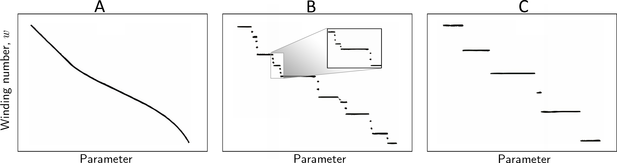
Figure 2: Illustration of commensurate-incommensurate transitions in periodic systems [3]. A. Continuous (analytical [21]) transition. B. Complete devil’s staircase. It has a (non-analytical [21]) fractal structure, such that the plateaus contain commensurate phases (rational $w$), and there are infinite plauteaus between every two plateaus. The incommensurate phases lie in between the commensurate phases (irrational $w$), making a set of zero measure in the parameter space. C. Harmless staircase. The system transitions discontinuously transitions from one commensurate $w$ to another. The incomplete devil’s staircase is similar to the harmless staircase, except that the transitions are continuous.

A slow-fast analysis of our model can be performed in the limit [4] $\delta=\lambda\ll 1$. This is also known as adiabatic approximation. In this case, the variable $z(t)$ becomes slow when compared to $x(t)$, and so it can be turned into a parameter and absorbed inside $H^{\prime}=H+z(t)$. This can be used to understand the emergence of cardiac oscillations in the model, since it can be shown that for $H^{\prime}=0$ and $T<K-2+1/K$, there is a coexistence of two stable fixed points [12]. These give rise to a hysteresis cycle as a function of $H^{\prime}$.

III Methods

The model undergoes an infinite-period bifurcation at [12] $x_{R}=-K+T$ (for small $\delta=\lambda$ and $H=0$). Thus, we fixed $K=0.6$, $\delta=\lambda=0.001$, $H=0$, and for each $(T,x_{R})$ pair, we iterated Eq. (1) for $200,000$ time steps, discarding the initial transient of $20,000$ steps. Near the bifurcation, longer simulation times may be required to observe our results. We used $x(0)=y(0)=z(0)=1.0$ as initial condition. Each attractor is characterized by three measurements: the sequence and distribution of the interspike interval (ISI), the Lyapunov exponent $L$, and the associated winding number $w$ (i.e., the ratio of cycles per period of the attractor).

III.1 Interspike interval

The interspike interval is the number of time steps between two consecutive upswings of the membrane potential $x(t)$ (see Fig. 1C). More precisely,

$$I\!S\!I_{n}=t_{n+1}-t_{n}$$ (2)

where the instants $t_{n}$ and $t_{n+1}$ are defined by the simultaneous conditions

$$\left\{\begin{array}[]{rl}x(t_{k}+1)x(t_{k})\leq 0&\textnormal{[the map crossed }x=0\\ &\textnormal{between }t_{k}\textnormal{ and }t_{k}+1\textnormal{]}\ ,\\ x(t_{k})<x(t_{k}+1)&\textnormal{[the oscillation is rising]}\ ,\end{array}\right.$$ (3)

taking $k=n$ for the spike at time $t_{n}$ and $k=n+1$ for the spike at time $t_{n+1}$. There is no other $t$ between $t_{n}$ and $t_{n+1}$ that obeys both of these conditions. In other words, $t_{n}$ and $t_{n+1}$ can be regarded as the timestamps of consecutive spikes. Repeating this for every spike produces the sequence $\{I\!S\!I_{n}\}$ illustrated in Fig. 1C.

Note that a given attractor can have more than one unique ISI in $\{I\!S\!I_{n}\}$. This is the case for bursting, for example, where there are at least two distinct values in the sequence: the smallest corresponds to the interval between spikes within a burst, and the largest corresponds to the interval between spikes in consecutive bursts. This produces the multimodal distributions of $I\!S\!I_{n}$ shown for the Burst and DAD attractors in Fig. 1B–right. Thus, in general, the $I\!S\!I_{n}$ are not the period of the attractor.

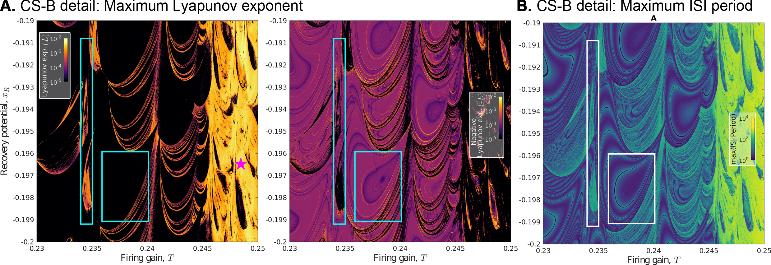
Figure 3: Detail of the dust-like structure in the CS-B transition. A. Maximum Lyapunov exponent calculated via the Eckmann-Ruelle procedure (see Methods). Colors: positive $L$ chaotic regions (left); negative $L$ non-chaotic regions (right). Maximum Lyapunov exponent colors (black to yellow) $\to$ $10^{-5}\leq-L<10^{-4}$ (black), $10^{-4}\leq-L<10^{-3}$ (purple-orange), $10^{-3}\leq-L<10^{-2}$ (yellow). Black gaps$\to$non-chaotic regions (all the Lyapunov exponents are negative). Star: selected DAD attractor shown in Fig. 4B–bottom. B. The maximum period of the $\{I\!S\!I_{n}\}$ sequence reveals the internal structure of the non-chaotic regions, closely matching the negative $L$ contour. ISI period colors (blue to yellow) $\to$ $P$ of $\{I\!S\!I_{n}\}$: $P=1$ to $P=10$ (blue shades); $P=10$ to $P=10^{2}$ (green shades); $P=10^{2}$ to $P=10^{3}$ (yellow shades). All panels: Rectangles $\to$ selected regions for further analysis in Figs. 4, 5 and 6. Taller rectangle on the left $\to$ Figs. 4A and 5C; Smaller rectangle on the right $\to$ Fig. 5B. Both rectangles also appear in Fig. 5A.

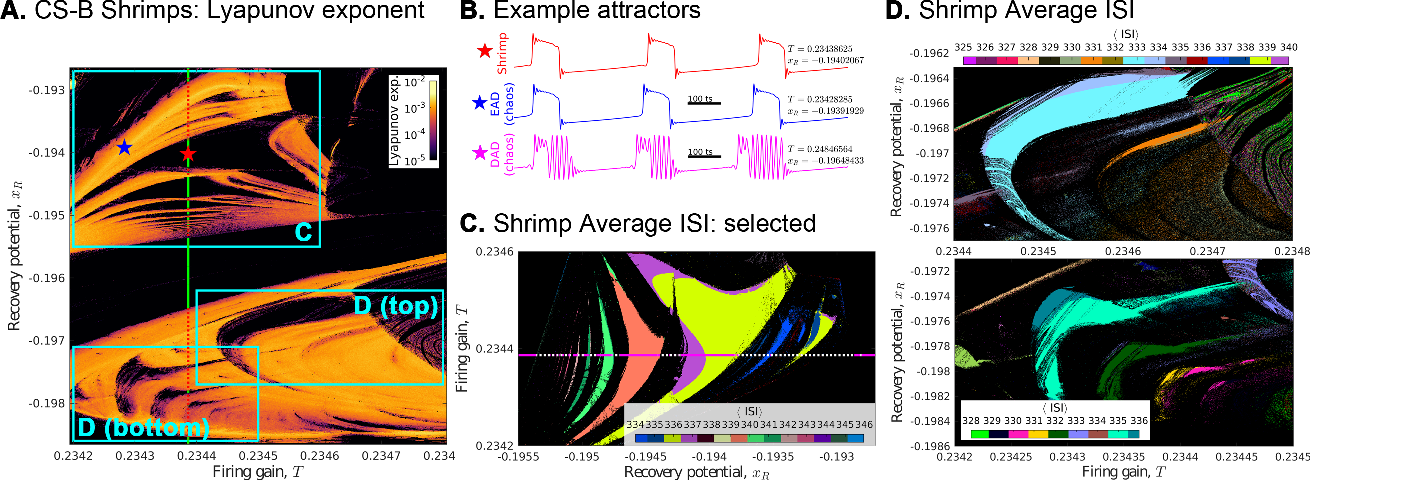
Figure 4: Shrimps viewed with average ISI. A. Detail of the region enclosed by the tall rectangle on the left in Fig. 3A: shrimps are nonchaotic regions (black$\to$all Lyapunov exponents negative) surrounded by a chaotic sea (colored region$\to$positive largest Lyapunov exponent). Rectangles highlight the regions shown in panels C and D. Stars: selected attractors for panel B. B. Selected attractors. EADs shows up both inside (top) and outside (middle) the shrimp. DAD shows mostly in chaotic regions (bottom, star shown in Fig. 3A). C and D. Each color corresponds to a unique $\left\lfloor\left\langle I\!S\!I\right\rangle\right\rceil$ ($\left\langle I\!S\!I\right\rangle$ rounded to the nearest integer – see Methods). The bulk region of shrimps have a single $\left\lfloor\left\langle I\!S\!I\right\rangle\right\rceil$, whereas the borders show a secondary $\left\lfloor\left\langle I\!S\!I\right\rangle\right\rceil$ resulting in a cascade of periods within and across shrimps. C. Sequence of shrimps selected for a detailed inspection of the ISI bifurcation and period cascade in Fig. 6. Horizontal line: selected $T=0.2343864$ value for the bifurcation analysis; the solid parts correspond to nonchaotic regions and are inside shrimps, and dotted parts are chaotic regions in between shrimps. Notice that here we are plotting $T$ vs. $x_{R}$ for better correspondence with the bifurcation diagrams in Fig. 6. The other panels have $x_{R}$ vs. $T$.

The discrete nature of time also introduces a $\pm 1$ variability for a given $I\!S\!I_{n}$ in the sequence $\{I\!S\!I_{n}\}$. This is because the conditions in Eq. (3) used to define $t_{n}$ and $t_{n+1}$ do not require the map to exactly repeat after the $t_{n+1}$ time step. Put differently, even if the waveform of the oscillation repeats after one ISI, the actual map value $x(t)$ does not need to do the same. This can be seen in the CS attractor in Fig. 1C: the attractor consists of the circles, and the spike timestamps $t_{n}$ are marked by a red “x” symbol which stands for $t_{1}$ in the first spike, $t_{2}$ in the second, and $t_{3}$ in the third. However, the values of the map [the circles marking $x(t_{1}+1)$, $x(t_{2}+1)$ and $x(t_{3}+1)$] following the timestamp are different for the three spikes (the distance of the circles to the $x=0$ dashed line increases during the spiking). This shifting of the map with respect to the waveform generates the $\pm 1$ variability that can be clearly seen in the ISI distribution for the CS and EAD attractors (Fig. 1B–right) – both of which have a steady waveform throughout which the actual values of the map slide.

Figure 5: Shrimps viewed with maximum ISI period and negative maximum Lyapunov exponent. ISI period colors (blue to yellow) $\to$ $P$ of $\{I\!S\!I_{n}\}$: $P=1$ to $P=10$ (blue shades); $P=10$ to $P=10^{2}$ (green shades); $P=10^{2}$ to $P=10^{3}$ (yellow shades); Negative maximum Lyapunov exponent colors (black to yellow) $\to$ $10^{-5}\leq-L<10^{-4}$ (black), $10^{-4}\leq-L<10^{-3}$ (purple-orange), $10^{-3}\leq-L<10^{-2}$ (yellow). A very similar contouring is obtained by both metrics (negative maximum Lyapunov exponent $-L$, and ISI period $P$), as also seen in Fig. 3A–right. A. Detail of Fig. 3B. The nonchaotic region shows loops of constant $P$. Rectangles show the regions displayed in panels B and C. B. Detail of the non-chaotic region loops of constant $P$ corresponding to the short rectangle of Fig. 3B. C. Shrimps region corresponding to the tall rectangle of Fig. 3B. Rectangles contain the regions displayed in panels D, E and F. D, E, F. Shrimps are nonchaotic regions and have inner stripes of constant $P$ similar to the loops observed in the other nonchaotic regions. E,F. Selected shrimp sequence corresponding to Fig. 4C used for the bifurcation diagrams of Fig. 6. Horizontal line: selected $T=0.2343864$ value for the bifurcation analysis; the solid parts correspond to nonchaotic regions and are inside shrimps, and dotted parts are chaotic regions in between shrimps. Notice that here we are plotting $T$ vs. $x_{R}$ for better correspondence with the bifurcation diagrams of Fig. 6. The stripes inside the shrimps correspond to the periodicity steps in the devil’s staircase of Fig. 2. The other panels have $x_{R}$ vs. $T$.

We can illustrate this variability effect with the Poincaré section of a simple cosine function $v(t)=\cos(2\pi t/Q)$ with actual period $Q=20$. Taking $v(t)$ only at integer $t\geq 1$, and applying it to the conditions in Eq. (3), produces the sequence $\{I\!S\!I_{n}\}=\{20,19,21,19,20,21,\cdots\}$. By construction, we know the correct ISI should be equal to $Q=20$, but values fluctuate. Sampling the series long enough, we can get $\left\langle I\!S\!I\right\rangle\approx Q=20$ in this example. The equality $\left\langle I\!S\!I\right\rangle\approx Q$ holds only for periodic functions that repeat at every cycle.

If the attractor $x(t)$ is periodic, then the sequence $\{I\!S\!I_{n}\}$ must be periodic. This follows because if $x(t)$ is periodic of period $Q$, then $x(t)=x(t+Q)$ for all $t$. In particular, this is true for any $t=t_{n}$ in the sequence of upward crossings. In other words, if the map crosses $x=0$ during a rise at $t=t_{n}$, it must also rise up at $t=t_{n+P}=t_{n}+Q$ after some integer number of cycles $P$. Therefore,

$$I\!S\!I_{n+P} =t_{n+1+P}-t_{n+P}$$

$$=t_{n+1}+Q-(t_{n}+Q)$$

$$=t_{n+1}-t_{n}=I\!S\!I_{n}\ ,$$

and $I\!S\!I_{n+P+1}=I\!S\!I_{n+1}$, and so on and so forth, making $P$ the period of the $\{I\!S\!I_{n}\}$ sequence. Consequently, the period of the attractor is

$$Q=\sum_{k=n}^{n+P}I\!S\!I_{k}\ ,$$ (4)

since $I\!S\!I_{k}$ is the duration of the $k$-th cycle of the map, and the map repeats after $P$ cycles. Also, if we iterate the map for a total of $mQ$ time steps ($m\gg 1$), the map executes $\left|\{I\!S\!I_{n}\}\right|=mP$ cycles, so the average ISI is

$$\left\langle I\!S\!I\right\rangle=\dfrac{1}{\left|\{I\!S\!I_{n}\}\right|}\sum_{k=1}^{\left|\{I\!S\!I_{n}\}\right|}I\!S\!I_{k}=\dfrac{mQ}{mP}=\dfrac{Q}{P}\ .$$ (5)

We also plot the ISI rounded to the nearest integer, $\left\lfloor\left\langle I\!S\!I\right\rangle\right\rceil$.

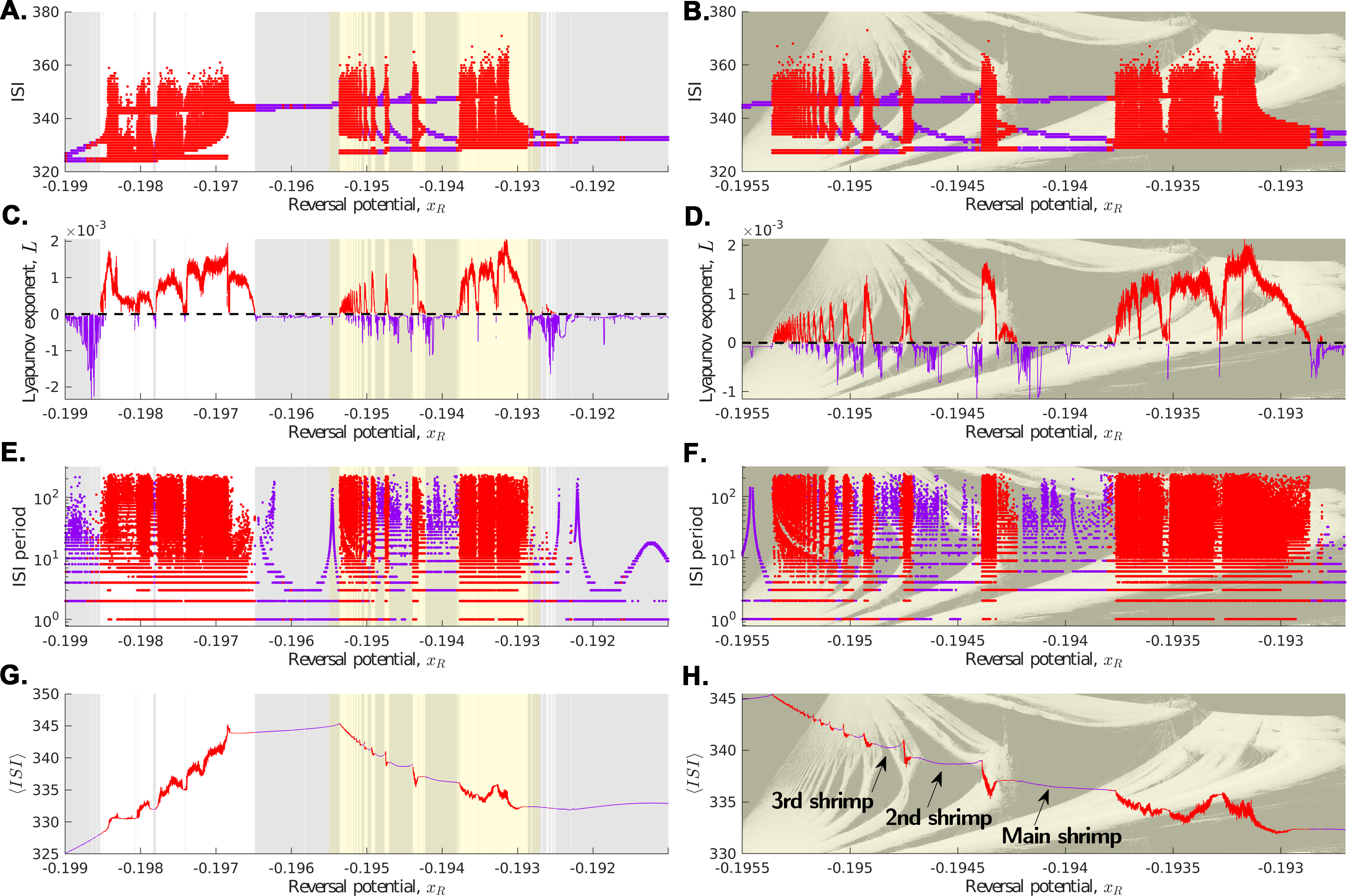
Figure 6: Shrimps’ ISI diagrams for fixed $T=0.2343864$. Left column$\to$traversing the parameter space over the solid-dotted lines shown in Figs. 4A and 5C (darker background$\to$nonchaotic regions where all Lyapunov exponents are negative). Left column yellow background$\to$selected $x_{R}$ range shown on the right column. Right column$\to$detail of the left column, traversing the shrimp sequence shown in Figs. 4C and 5E,F along the horizontal dotted-solid line shown there. We plot the shrimps’ silhouette on the background to make this clear. Red curves$\to$positive maximum Luapunov exponents (chaotic attractors); purple curves$\to$all Lyapunov exponents are negative. A and B. ISI bifurcation diagrams showing that attractors inside the shrimps (darker yellow background) can have more than one value in the $\{I\!S\!I_{n}\}$ sequence (e.g., the main shrimp has three distinct ISI’s between 330 and 350 ts). C and D. The maximum Lyapunov exponent shows chaotic regions in between shrimps. E and F. The $\{I\!S\!I_{n}\}$ has multiple periods $P$ inside shrimps (ranging from $P=1$ where attractors repeat at every oscillation, to $P\sim 200$). G and H. $\left\langle I\!S\!I\right\rangle$ is shown without rounding, revealing a slight variation inside shrimps (pointed by arrows, further analyzed in Fig 7), and forming a harmless staircase going from one shrimp to another.

III.2 Winding number

The winding number $w$ is defined as the number of cycles $P$ executed by the map during a single period of oscillation $Q$. The derivation of Eq. (5) implies that

$$w=\dfrac{P}{Q}=\dfrac{1}{\left\langle I\!S\!I\right\rangle}\ .$$ (6)

Rational $w$ implies in phases where $P$ and $Q$ are commensurable, i.e., we can always find an interval of time $mQ$ inside which lie $mP$ cycles of the oscillation. Conversely, irrational $w$ implies in an incommensurate oscillation. Incommensurate phases can be sliding or locked. The sliding case means that the attractor $x(t)$ can assume any real value in the range $(-1;1)$. Locked attractors exist only in restricted subintervals of this range.

The transition between commensurate and incommensurate phases has been studied in the context of spatial ordering in magnets and other systems [21, 3, 22, 23, 24], including in the original version of our model where $F(u)=\tanh(u)$ and $x(t)$ is the magnetization at inner layer $t$ of the Bethe lattice [5, 6]. As a single parameter is varied, the transition can be continuous, discontinuous, or quasi-continuous (see Fig. 2). Here, we study $w$ as a function of $x_{R}$ with all the other parameters kept fixed.

A continuous transition is known as analytical [21], where the system goes smoothly from one $w$ to another without staying trapped in a single $w$ as the parameter is varied (Fig. 2A). On the other end, discontinuous transitions are characterized by the system jumping from a commensurate phase to another, and there are only finitely many commensurate phases in the considered parameter range (Fig. 2C). A complete devil’s staircase is when there are infinitely many commensurate phases in the considered parameter range, and hence $w$ varies non-analytically (Fig. 2B). In this case, incommensurate phases lie in a set of zero measure in the parameter space, making the complete devil’s staircase a sort of Cantor fractal [22]. We estimate the fractal dimension $D_{f}$ by the standard box-size scaling procedure [25]: the plot is divided into boxes of size $s$ and we count the number of boxes that contain a data point, and repeat this for various box sizes $s$. The slope of the log-log count vs. $s$ curve is approximately $D_{f}$.

The steps in a complete devil’s staircase can make a nonstandard Farey sequence [9, 26]. This means given two steps, one with $w_{1}=P_{1}/Q_{1}$ and the other with $w_{2}=P_{2}/Q_{2}$, there is a third step in between with $w_{3}=P_{3}/Q_{3}$, such that $P_{3}=P_{1}+P_{2}$ and $Q_{3}=Q_{1}+Q_{2}$. This is true for any two steps in the staircase.

III.3 Lyapunov exponent

The Jacobian matrix is defined by the elements $(\mathbf{J}_{t})_{ij}=\partial\mathbf{x}_{i}(t+1)/\partial\mathbf{x}_{j}(t)$, with $i$ and $j$ equal to $1$, $2$, or $3$, where $\mathbf{x}_{i}(t)$ is the $i$-th component of $\mathbf{x}$ at time $t$ ($\mathbf{x}_{1}=x$; $\mathbf{x}_{2}=y$; $\mathbf{x}_{3}=z$),

$$\mathbf{J}_{t}=\left[\begin{array}[]{ccc}\frac{1}{T}F^{\prime}\!\left(u(t)\right)&-\frac{K}{T}F^{\prime}\!\left(u(t)\right)&\frac{1}{T}F^{\prime}\!\left(u(t)\right)\\ 1&0&0\\ -\lambda&0&1-\delta\end{array}\right]\ ,$$ (7)

with $u(t)=[x(t)-Ky(t)+z(t)+H]/T$.

The Lyapunov exponents are given by

$$L_{i}=\lim_{\tau\to\infty}\dfrac{1}{\tau}\ln|\Lambda_{i}|\ ,$$ (8)

where $\Lambda_{i}$ are the eigenvalues of the product $\mathbf{L}$ of the Jacobian matrices evaluated at each time $t$ from $1$ to $\tau$,

$$\mathbf{L}=\mathbf{J}_{\tau}\mathbf{J}_{\tau-1}\cdots\mathbf{J}_{t}\cdots\mathbf{J}_{2}\mathbf{J}_{1}\ .$$

If the largest exponent, $L=\max_{i}L_{i}>0$, then the attractor is said to be chaotic. Otherwise, $L\leq 0$ is found for periodic or quasi-periodic orbits, with $L<0$ in dissipative systems.

This calculation in Eq. (8) is computationally expensive and can be approximated using the Eckmann-Ruelle method [27]. It consists of diagonalizing each Jacobian matrix that makes up $\mathbf{L}$, such that

$$\mathbf{A}_{t}\mathbf{B}_{t}=\mathbf{J}_{t}\mathbf{A}_{t-1}\ ,$$

$\mathbf{A}_{0}=\mathbf{1}$ is the identity matrix, and $\mathbf{A}$ and $\mathbf{B}$ are lower and upper triangular matrices, respectively, obtained by LU decomposition. Thus, we can write $\mathbf{L}$ as

$$\mathbf{L}=(\mathbf{A}_{\tau}\mathbf{B}_{\tau}\mathbf{A}_{\tau-1}^{-1})(\mathbf{A}_{\tau-1}\mathbf{B}_{\tau-1}\mathbf{A}_{\tau-2}^{-1})\cdots\\ \cdots(\mathbf{A}_{t+1}\mathbf{B}_{t+1}\mathbf{A}_{t}^{-1})(\mathbf{A}_{t}\mathbf{B}_{t}\mathbf{A}_{t-1}^{-1})\cdots\\ \cdots(\mathbf{A}_{3}\mathbf{B}_{3}\mathbf{A}_{2}^{-1})(\mathbf{A}_{2}\mathbf{B}_{2}\mathbf{A}_{1}^{-1})(\mathbf{A}_{1}\mathbf{B}_{1})\\ =\mathbf{A}_{\tau}\mathbf{B}_{\tau}\mathbf{B}_{\tau-1}\cdots\mathbf{B}_{t}\cdots\mathbf{B}_{2}\mathbf{B}_{1}\\ \approx\mathbf{B}_{\tau}\mathbf{B}_{\tau-1}\cdots\mathbf{B}_{t}\cdots\mathbf{B}_{2}\mathbf{B}_{1}\ .$$

The Lyapunov exponents are then approximated by

$$L_{i}\approx\dfrac{1}{\tau}\sum_{t=1}^{\tau}\ln\left|\left(\mathbf{B}_{t}\right)_{ii}\right|\ ,\ \left(i=1,2,3\textnormal{ for }x,y,z\right)\ ,$$ (9)

where $\tau$ is a long time (e.g., $\sim 10^{7}$ ts), and $\left(\mathbf{B}_{t}\right)_{ii}$ are the diagonal elements of the upper triangular matrix $\mathbf{B}_{t}$.

IV Results

The phase diagram of oscillation modes, Fig. 1A, was colored by classifying the attractors through their ISI distribution (see [12] for details). This revealed a dust-like structure in the boundary between the CS and B transition. CS transforms into B passing through a delayed Neimark-Sacker bifurcation, making the plateau unstable and, eventually, generating afterdepolarization spikes [4]. These transition attractors, labeled as EAD and DAD in Fig. 1B,C, are present in heart myocytes when patients display cardiac arrhythmia [1, 2]. In our map, DADs are typically chaotic, whereas EADs are usually periodic. Here, we investigate what is the structure of the dusty region in the transition between CS and B, and characterize the periodicity of its corresponding attractors.

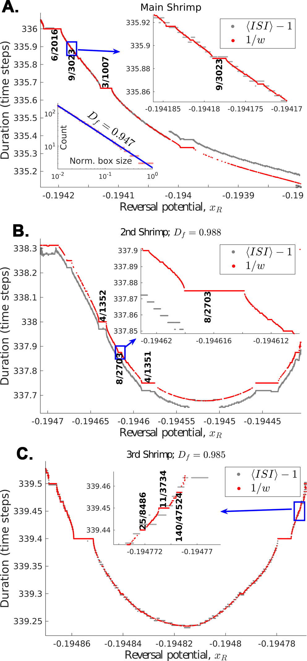
Figure 7: Shrimps’ complete devil’s staircases. Detail of the $\left\langle I\!S\!I\right\rangle$ data pointed by arrows in Fig. 6H compared to the inverse winding number, $1/w=Q/P$. Some staircase steps are labeled by $w=P/Q$ to highlight the Farey tree structure of the system. Each panel has $x_{R}$ crossing the shrimp at fixed $T=0.2343864$. $\left\langle I\!S\!I\right\rangle-1$ is approximately equal to $1/w$ due to the $\pm 1$ intrinsic variability of the $\left\langle I\!S\!I\right\rangle$ discussed in Methods. The steps in the staircase are the stripes of the maximum ISI period and maximum negative Lyapunov exponent shown in and 5E,F. The analysis here is valid for all the shrimps that we show in this manuscript. A. Main shrimp (largest one in the sequence). A (bottom inset). Box count metric used to estimate the fractal dimension of the staircase. B. Second shrimp (first to the left of the main one). C. Third shrimp (second to the left of the main one). Top insets. Detail of the main panel inside the drawn rectangle.

IV.1 ISI sequence reveals structure of non-chaotic regions

Zooming in the dust using the Lyapunov exponent, we can see islands of periodic non-chaotic behavior forming twisted half-moon shapes (Fig. 3A). These shapes prevail for $T<0.243$, which is the value of $T$ in which oscillations first appear in the slow-fast description of the model [4] obtained when $\delta=\lambda\ll 1$. The maximum period of the $\{I\!S\!I_{n}\}$ reveals that these non-chaotic regions form rings of isoperiodic ISI sequences (Fig. 3B). The period of $\{I\!S\!I_{n}\}$ of chaotic attractors is also large. However, this is only due to the finite simulation time. The more time we iterate the model, the larger the period of the ISI sequence of chaotic attractors due to its aperiodic nature.

Squeezed between the half-moon shapes, there are different sequences of shrimps (Fig. 4A). Shrimps are regions in the parameter space throughout which attractors have the same period [15, 16]. It is worth noticing that we are calling these structures as shrimps because they resemble those originally found in the Hénon map [15]. However, our map has three variables making a slow-fast dynamic and a cubic nonlinearity due to the sigmoid shape of $F(u)$, whereas the Hénon map is a two-variable quadratic equation with a single time scale. Also, the oscillatory behavior of the attractors we are studying (CS, EAD, DAD and B) require the slow-fast dynamic to exist, and hence can have multiple ISI in the $\{I\!S\!I_{n}\}$. With this in mind, we selected three sequences of shrimps to further explore in details.

IV.2 Shrimps have two rounded average ISI

Rounding the ISI of the attractors, we can assign a single label $\left\lfloor\left\langle I\!S\!I\right\rangle\right\rceil$ to the bulk of each shrimp, whereas their borders have a secondary $\left\lfloor\left\langle I\!S\!I\right\rangle\right\rceil$ (Fig. 4C,D). The shrimps decrease in shape together with a slowly growing sequence of $\left\lfloor\left\langle I\!S\!I\right\rangle\right\rceil$.

IV.3 Shrimps have multiple periodicity of the ISI sequence

One can argue that rounding the average ISI may hide important information about the nature of the attractors. Thus, we also look at the sequence of ISI (Fig. 5). Similarly to what happens inside the half-moon regions, shrimps show multiple periods of the $\{I\!S\!I_{n}\}$ sequence (Fig. 5C,D,E,F). However, the isoperiodic regions of $\{I\!S\!I_{n}\}$ form stripes inside the shrimps instead of rings. These strips correspond to steps in the devil staircase.

IV.4 ISI bifurcation and the devil’s staircase

In order to detail the dynamics inside and around the shrimps, we fixed $T=0.2343864$ and varied $x_{R}$ throughout the main shrimp sequence shown in Figs. 4A,C and 5C,E,F. Along this fixed $T$ line, we plot the ISI bifurcation diagram (Fig. 6A,B), the maximum Lyapunov exponent (Fig. 6C,D), the period of the ISI sequence (Fig. 6E,F), and the average ISI (Fig. 6G,H).

All the shrimps in the sequence three or more distinct ISIs (Fig. 6A,B) ranging from, approximately, 330 to 350 time steps. The largest (main) shrimp has three ISIs. In the second and third largest shrimps, the upper ISI starts branching out as $|x_{R}|$ decreases towards the main shrimp (Fig. 6B). This organization seems to be intimately related to the nearby chaos. This is because the periodic regions farther from the shrimps (darker shaded regions in Fig. 6A) have single ISIs.

The period of the $\{I\!S\!I_{n}\}$ sequence is shown in Figs. 6E,F. As explained in Methods, each $I\!S\!I_{n}$ in the sequence may show a slight variation of $\pm 1$ due to the discrete nature of the map with respect to the waveform. This means that some of the data shown in these panels are due to these random fluctuations. The maximum period of the sequence is more reliable because the period due to random fluctuations become neglible as the period of the sequence grows. Farther from the shrimp region, the periodic regions display a more well-behaved period of the ISI sequence. Inside the shrimps, the period of the ISI sequence shows multiple values, although not as many as in the chaotic regions.

We show the $\left\langle I\!S\!I\right\rangle$ without rounding Figs. 6G,H. The regions in between shrimps show a spurious $\left\langle I\!S\!I\right\rangle$ due to the aperiodic behavior of the attractors. From one shrimp to the other, starting from the largest one and going to the direction of growing $|x_{R}|$, we can see the increasing sequence of $\left\langle I\!S\!I\right\rangle$ as steps in a harmless staircase, confirming the findings with rounded ISI in Fig. 4C. However, we can see a slight slope for the $\left\langle I\!S\!I\right\rangle$ inside the shrimp. This is particularly noticeable in the first three shrimps pointed by arrows.

Fig. 7 shows the detail of the $\left\langle I\!S\!I\right\rangle$ for the first three shrimps compared to the inverse winding number $1/w=Q/P$. The whole extent of each panel is inside a shrimp, so the staircases appear as features of the shrimps themselves. We expect that $\left\langle I\!S\!I\right\rangle=1/w$ [Ex. (6)]. In the three panels, we can se that both the $\left\langle I\!S\!I\right\rangle$ and the $1/w$ curves match almost completely. However, again there are fluctuations in $I\!S\!I_{n}$, such that a better match between both quantities was only obtained by taking $\left\langle I\!S\!I\right\rangle-1$.

The $\left\langle I\!S\!I\right\rangle$ is much easier to measure, and provides a great estimate of $1/w$, even though more precise fractal dimensions and attractor labels can only be obtained from the $1/w$ curve. We found fractal dimensions of about $D_{f}\sim 0.95$ for the main shrimp and $D_{f}\sim 0.98$ for the other two, meaning that the staircase is tightly packed with periodic attractors. The gaps in the staircases are due only to the finite simulation time.

The whole staircase fits inside one unit of $\left\langle I\!S\!I\right\rangle$ because the period $Q$ of each attractor is relatively large compared to the number of cycles. This is a direct consequence of the slow time scale that makes up the plateau spikes. Increasing $\delta=\lambda$ destroys the plateaus and would possibly disrupt the findings we describe here. We highlighted a few winding number $w$ labels in each shrimp to show that the staircase generates a Farey tree sequence. For example, the three labeled steps in the main shrimp have $w_{1}=6/2016$, $w_{2}=3/1007$ and $w_{3}=(6+3)/(2016+1007)=9/3023$ (the step between $w_{1}$ and $w_{2}$). The same follows for all the other steps. The second and third shrimps (Fig. 7B,C) have non-monotonic staircases.

V Conclusion

We studied a three-variable map that can be employed in different areas: from magnets to membrane voltage models. In particular, the homeostatic field $z(t)$ introduces a slow-fast dynamic that is capable of generating plateau spikes and bursts. The transition between these regimes is permeated by a loss of stability of the plateau, generating early and delayed afterdepolarizations of the membrane. This behavior is found in some cardiac arrhythmias due to impairment in ionic channels [28, 29]. For example, delayed sodium currents can prolong the AP, enabling calcium currents to destabilize repolarization and cause EADs [30, 31]. Sodium-triggered EADs and DADs can occur without altering AP duration [32]. Compromised slow potassium currents are critical for AP prolongation and the emergence of EADs or DADs [28, 29].

In our model, slow currents are captured by $z(t)$ while fast negative feedback is captured by $y(t)$. Since the parameters are dimensionless, we are free to interpret in different ways. For example, the parameter $K$ controls the fast negative feedback, and can play the role of a sodium conductance. On the other hand, $\delta$ plays the role of the recovery time scale of the slow current. The parameter $x_{R}$ is the reversal potential of the slow current, and we predict that cardiomyocytes can undergo multiple periodicity changes via a devil’s staircase as their potassium reversal potential is shifted towards EAD behavior.

Recent work revealed that shrimps can exhibit quasi-periodic dynamics, characterized by torus-bubbling transitions and multi-tori attractors [17], contrasting with the period-doubling mechanisms of periodic shrimps [15]. Building on this, we showed that shrimps in our model contain internal stripe-like structures, each with a constant period. When plotted against a single parameter, these stripes form a complete devil’s staircase, uncovering a novel organizational feature of shrimp dynamics. This means that along the CS-B transition, the membrane potential undergoes a series of infinite periodicity changes before reaching a bursting regime. Some of these changes result in EADs and DADs.

EADs can be linked to chaos [33, 34]. In our model, this is not necessary [4]. Although EADs and DADs develop near a chaotic transition into bursting, EADs can be both periodic (existing inside a shrimp) or chaotic. DADs, on the other hand, are frequently chaotic, existing in between shrimps.

Cardiac arrhythmias are a leading cause of heart failure worldwide, driven by disruptions in cardiac myocyte action potentials. Our study’s simplicity and broad applicability enable experimental validation, enhance diagnostics, and support the development of better tools to treat and prevent cardiac dysfunction.

Data availability statement

Simulations are available in
https://github.com/mgirardis/ktz-phasediag

Declaration of interests

The authors declare no competing interests.

References

References

- Yan et al. [2001] G. Yan, Y. Wu, T. Liu, J. Wang, R. A. Marinchak, and P. R. Kowey, Phase 2 Early Afterdepolarization as a Trigger of Polymorphic Ventricular Tachycardia in Acquired Long-QT Syndrome: Direct Evidence From Intracellular Recordings in the Intact Left Ventricular Wall, Circulation 103, 2851 (2001).
- Katz [2011] A. M. Katz, Physiology of the heart, 5th ed. (Lippincott Williams & Wilkins, 2011).
- Bak [1982] P. Bak, Commensurate phases, incommensurate phases and the devil’s staircase, Reports on Progress in Physics 45, 587 (1982).
- Morelo et al. [2024] P. A. Morelo, M. Girardi-Schappo, B. L. Paulino, B. Marin, and M. H. R. Tragtenberg, Recovering from cardiac action potential pathologies: a dynamic view, Research Square PREPRINT, 10.21203/rs.3.rs (2024).
- Yokoi, de Oliveira, and Salinas [1985] C. S. O. Yokoi, M. J. de Oliveira, and S. R. Salinas, Strange Attractor in the Ising Model with Competing Interactions on the Cayley Tree, Phys. Rev. Lett. 54(3), 163 (1985).
- Tragtenberg and Yokoi [1995] M. H. R. Tragtenberg and C. S. O. Yokoi, Field behavior of an Ising model with competing interactions on the Bethe lattice, Phys. Rev. E 52(3), 2187 (1995).
- Lombardi et al. [2023] F. Lombardi, S. Pepić, O. Shriki, G. Tkačik, and D. De Martino, Statistical modeling of adaptive neural networks explains co-existence of avalanches and oscillations in resting human brain, Nature Computational Science 3, 254 (2023).
- Clark and Abbott [2024] D. G. Clark and L. F. Abbott, Theory of Coupled Neuronal-Synaptic Dynamics, Phys. Rev. X 14, 021001 (2024).
- Kinouchi and Tragtenberg [1996] O. Kinouchi and M. H. R. Tragtenberg, Modeling neurons by simple maps, Int. J. Bifurcat. Chaos 6, 2343 (1996).
- Kuva et al. [2001] S. M. Kuva, G. F. Lima, O. Kinouchi, M. H. R. Tragtenberg, and A. C. Roque, A minimal model for excitable and bursting elements, Neurocomputing 38–40, 255 (2001).
- Girardi-Schappo, Tragtenberg, and Kinouchi [2013] M. Girardi-Schappo, M. Tragtenberg, and O. Kinouchi, A brief history of excitable map-based neurons and neural networks, J. Neurosci. Methods 220, 116 (2013).
- Girardi-Schappo et al. [2017] M. Girardi-Schappo, G. S. Bortolotto, R. V. Stenzinger, J. J. Gonsalves, and M. H. R. Tragtenberg, Phase diagrams and dynamics of a computationally efficient map-based neuron model, PLoS ONE 12, e0174621 (2017).
- Stenzinger and Tragtenberg [2022] R. V. Stenzinger and M. H. R. Tragtenberg, Cardiac reentry modeled by spatiotemporal chaos in a coupled map lattice, Eur. Phys. J. Spec. Top. 231, 847 (2022).
- Bortolotto, Stenzinger, and Tragtenberg [2019] G. S. Bortolotto, R. V. Stenzinger, and M. H. R. Tragtenberg, Electromagnetic induction on a map-based action potential model, Nonlinear Dynamics 95, 433 (2019).
- Gallas [1993] J. A. C. Gallas, Structure of the parameter space of the Hénon map, Phys. Rev. Lett. 70, 2714 (1993).
- Gallas [1994] J. A. C. Gallas, Dissecting shrimps: results for some one-dimensional physical models, Physica A 202, 196 (1994).
- Pati [2024] N. C. Pati, Spiral organization of quasi-periodic shrimp-shaped domains in a discrete predator-prey system, Chaos 34, 083126 (2024).
- Balaraman et al. [2023] S. Balaraman, S. N. Dountsop, J. Kengne, and K. Rajagopal, A circulant inertia three Hopfield neuron system: dynamics, offset boosting, multistability and simple microcontroller- based practical implementation, Physica Scripta 98, 075224 (2023).
- FitzHugh [1960] R. FitzHugh, Thresholds and Plateaus in the Hodgkin-Huxley nerve equations, The Journal of General Physiology 43, 867 (1960).
- Teka et al. [2011] W. Teka, K. Tsaneva-Atanasova, R. Bertram, and J. Tabak, From Plateau to Pseudo-Plateau Bursting: Making the Transition, Bull. Math. Biol. 73, 1292 (2011).
- Aubry [1978] S. Aubry, in Solitons and Condensed Matter Physics (Springer-Verlag, Oxford, England, 1978) pp. 264–277.
- Bak [1986] P. Bak, The Devil’s Staircase, Physics Today 39, 38 (1986).
- Fischer et al. [1978] P. Fischer, G. Meier, B. Lebech, B. D. Rainford, and O. Vogt, Magnetic phase transitions of CeSb. I. Zero applied magnetic field, Journal of Physics C: Solid State Physics 11, 345 (1978).
- Kuroda et al. [2020] K. Kuroda, Y. Arai, N. Rezaei, S. Kunisada, S. Sakuragi, M. Alaei, Y. Kinoshita, C. Bareille, R. Noguchi, M. Nakayama, S. Akebi, M. Sakano, K. Kawaguchi, M. Arita, S. Ideta, K. Tanaka, H. Kitazawa, K. Okazaki, M. Tokunaga, Y. Haga, S. Shin, H. S. Suzuki, R. Arita, and T. Kondo, Devil’s staircase transition of the electronic structures in CeSb, Nat. Comm. 11, 2888 (2020).
- Falconer [2004] K. Falconer, Fractal Geometry: Mathematical Foundations and Application (John Wiley and Sons, USA, 2004).
- Perez, Sinha, and Cerdeira [1991] G. Perez, S. Sinha, and H. A. Cerdeira, Nonstandard Farey Sequences in a Realistic Diode Map, Europhysics Letters 16, 635 (1991).
- Eckmann and Ruelle [1985] J.-P.-P. Eckmann and D. Ruelle, Ergodic theory of chaos and strange attractors, Rev. Mod. Phys. 57, 617 (1985).
- J. [2007] V. J., The Long QT Syndrome, Heart Lung Circ 16 Suppl 3, S5 (2007).
- Varró and Baczkó [2011] A. Varró and I. Baczkó, Cardiac ventricular repolarization reserve: a principle for understanding drug-related proarrhythmic risk, Br J Pharmacol 164, 14 (2011).
- Zeng and Rudy [1995] J. Zeng and Y. Rudy, Early afterdepolarizations in cardiac myocytes: mechanism and rate dependence, Biophys J 68, 949 (1995).
- Greer-Short et al. [2017] A. Greer-Short, S. A. George, S. Poelzing, and S. H. Weinberg, Revealing the Concealed Nature of Long-QT Type 3 Syndrome, Circ Arrhythm Electrophysiol 10, e004400 (2017).
- Koleske et al. [2018] M. Koleske, I. Bonilla, J. Thomas, N. Zaman, S. Baine, B. C. Knollmann, R. Veeraraghavan, S. Györke, and P. B. Radwański, Tetrodotoxin-sensitive Navs contribute to early and delayed afterdepolarizations in long QT arrhythmia models, J Gen Physiol 150, 991 (2018).
- Tran et al. [2009] D. X. Tran, D. Sato, A. Yochelis, J. N. Weiss, A. Garfinkel, and Z. Qu, Bifurcation and Chaos in a Model of Cardiac Early Afterdepolarizations, Phys. Rev. Lett. 102, 258103 (2009).
- Weiss et al. [2010] J. N. Weiss, A. Garfinkel, H. S. Karagueuzian, P. Sheng Chen, and Z. Qu, Early afterdepolarizations and cardiac arrhythmias, Heart Rhythm 7(12), 1891 (2010).