Connections between sequential Bayesian inference and evolutionary dynamics

Abstract

It has long been posited that there is a connection between the dynamical equations describing evolutionary processes in biology and sequential Bayesian learning methods. This manuscript describes new research in which this precise connection is rigorously established in the continuous time setting. Here we focus on a partial differential equation known as the Kushner-Stratonovich equation describing the evolution of the posterior density in time. Of particular importance is a piecewise smooth approximation of the observation path from which the discrete time filtering equations, which are shown to converge to a Stratonovich interpretation of the Kushner-Stratonovich equation. This smooth formulation will then be used to draw precise connections between nonlinear stochastic filtering and replicator-mutator dynamics. Additionally, gradient flow formulations will be investigated as well as a form of replicator-mutator dynamics which is shown to be beneficial for the misspecified model filtering problem. It is hoped this work will spur further research into exchanges between sequential learning and evolutionary biology and to inspire new algorithms in filtering and sampling.

1 Introduction

It has been posited that there is a connection between sequential Bayesian inference and dynamical models describing evolutionary biological processes. Understanding and studying this connection has the potential to provide valuable insights on improved algorithms for complex Bayesian inference and sampling tasks arising in a wide range of fields in the data science, engineering and machine learning. Specifically, the key connection to sequential Bayesian estimation is via the so-called replicator-mutator partial differential equations [Kim24, Hof85], describing the time evolution of a large population of individuals with certain traits or attributes due to mutation and reproduction (or selection). Broadly speaking, sequential Bayesian estimation procedures bear striking similarity to the way species respond to evolutionary pressure moderated by a fitness landscape. The correspondence is as follows:

• states or parameters $\leftrightarrow$ traits

• prior distribution $\leftrightarrow$ current population

• prediction (in the case of filtering or hidden markov models) $\leftrightarrow$ mutation

• likelihood function $\leftrightarrow$ fitness landscape governing selection or birth-death

This connection has been discussed most notably in [Mor97, Sha09, Har09a, Aky17, Czé+22], primarily in the context of discrete time and discrete trait space problems. Some of the earliest connections between discrete time particle based Bayesian updating and genetic mutation-selection models seem to have been in e.g. [Mor97, Mor04, DG05]. [Sha09] raised awareness to the similarity to replicator equations specifically; they show how Bayesian updating corresponds to one step of a discrete-time and continuous-trait replicator equation without mutation. Around the same time, a similar point was made in [Har09a]. This connection to replicator equations with mutation was further extended to the setting of sequential in time inference with hidden Markov models (also known as sequential filtering, discrete time data assimilation)) in [Aky17, Czé+22]. They showed that discrete time replicator-mutator dynamics consists of a sequence of (discrete in time) alternating mutation and updating steps, as in sequential filtering. The PhD thesis [Zha17] draws some interesting connections to optimisation and interacting particle approaches to sequential filtering, e.g. the Feedback Particle Filter [Yan+12, Lau+14]. In this manuscript we focus on making this connection precise in the continuous time and continuous trait space case, which has not yet been explored thoroughly in the literature. More recently, there has been interest in incorporating replicator or “birth-death” dynamics into sampling algorithms for optimisation and inversion tasks, see e.g. [LLN19, LSW23, Che+24].

1.1 Replicator-mutator equations

The replicator-mutator equation is a broad class of dynamical systems modelling the response of a distribution of traits to evolutionary adaptation to an external fitness landscape. Early research on this class of models started with [Kim65, CK70] (sometimes also known as the Crow-Kimura equation), followed up by influential work in [Aki79, SS83] and many others. In these early works, the trait is often considered to be discrete (corresponding to discrete gene loci with a finite number of alleles) in the form $\dot{\pi}_{t}(i)=\pi_{t}(i)\left(\sum_{j}w_{ij}\pi_{t}(j)-\sum_{rs}w_{rs}\pi_{t}(r)\pi_{t}(s)\right)$, where $\pi_{t}$ is a $n$ dimensional probability vector of the relative frequency of each discrete trait, the matrix entries $w_{ij}$ record the fitness benefit (or harm) of the presence of trait $j$ for the proliferation of trait $i$, often assumed to be symmetric. The second term in the brackets ensures that $\pi\in S^{n}$, an $n$-dimensional probability simplex, i.e., $\pi(i)\geq 0$ and $\sum_{i}\pi(i)=1$ for all times. The dynamical properties of this system have been studied extensively see, e.g., [Bom90, OR01] and its relation to Fisher information and entropy has been studied in [BP16, Bae21]. This system also has a geometrical structure amenable to optimisation, as it can be seen to be a gradient flow of the total fitness with respect to the Shashahani metric, see [Har09, Har09a, FA95, Cha+21]. There is also a rich connection to game theory, as in [CT14] (with traits being interpreted as game strategies). The continuous trait space setting has received comparatively less attention, but has been studied as early as [Kim65] or in [CHR06, Gil+17, Vla20]. These models are popular in the mathematical evolution, biology, and ecology literature, primarily in discrete time, as in [KM14, KNP18, MHK14]. Nevertheless, the continuous time form of these models has been subject to attention from a mathematical analysis perspective [CS09, Cha+20]. The unnormalised or normalised form of the continuous-time continuous-trait replicator-mutator partial differential equations (PDEs) is given by

$$\partial_{t}\mu_{t}(x) =\mu_{t}(x)\mathbb{E}_{z\sim\mu_{t}}[f_{t}(x,z)]+\mathcal{L}^{\star}\mu_{t}(x)$$ (1.1)

$$\partial_{t}\rho_{t}(x) =\rho_{t}(x)\left(\mathbb{E}_{z\sim\rho_{t}}[f_{t}(x,z)]-\mathbb{E}_{\rho_{t}}[f_{t}]\right)+\mathcal{L}^{\star}\rho_{t}(x),$$ (1.2)

where $\rho_{t}(x)\geq 0$ and $\mu_{t}(x)\geq 0$ denote the normalised and unnormalised density functions respectively, describing the distribution of traits $x\in\mathbb{R}^{n}$ in the population. Here, $\mathcal{L}^{\star}q_{t}(x)$ is an optional mutation term, where $\mathcal{L}^{\star}$ is the adjoint generator of a diffusion process, e.g., $\mathcal{L}^{\star}=-\Delta$ for mutation according to standard Brownian motion. If $\mathcal{L}^{\star}=0$, i.e., no mutation exists, we call this the (pure) replicator equation. The (potentialy non-local & time-dependent) selection or fitness function is denoted by $f_{t}(x,z)$ and the net birth-death rate for a given trait $x$ at time $t$ is given by $\mathbb{E}_{z\sim\rho_{t}}[f_{t}(x,z)]$, where the subscript indicates that only the expectation is taken over the $z$ variable only. A simplified form of the replicator-mutator often appearing in the literature [TLK96, AC14, AC17] is the local PDE

$$\partial_{t}\rho_{t}(x) =\rho_{t}(x)\left(f_{t}(x)-\mathbb{E}_{\rho_{t}}[f_{t}]\right)+\mathcal{L}^{\star}\rho_{t}(x),$$ (1.3)

where the non-local fitness function in (1.2) has been replaced by a fitness function that no longer depends on the current distribution of traits, only on the value of the trait itself. An ubiquitous example is the quadratic fitness, $f_{t}(x)=-\frac{1}{2}\|Hx-y_{t}\|_{\Xi}^{2}$, which penalises traits $x$ that have a large misfit to the (potentially) time varying data $y_{t}$, is connected to least-squares estimation. The general idea here is that $H$ maps traits $x\in X$ to features $Hx\in Y$, and $y_{t}$ represents an optimal feature at time $t$, with fitness being quantified as a quadratic deviation, possibly preconditioned with a covariance matrix $\Xi$. A non-local version of this fitness function has been presented in [CHR06], i.e.

$$f_{t}(x,z)=-\frac{r}{2}\|Hx-y_{t}\|_{\Xi}^{2}-\frac{r}{2}\|Hz-y_{t}\|_{\Xi}^{2}+s\langle Hx-y_{t},Hz-y_{t}\rangle_{\Xi}$$ (1.4)

with $r>0,\,s<r$ (the case $H=I,r=1,y_{t}=0$ was presented in [CHR06]). This fitness function takes into account both a given trait’s fitness on its own, but also beneficial or adversary effects of the group fitness through the $s\langle Hx-y_{t},Hz-y_{t}\rangle_{\Xi}$ term. This non-local fitness function is studied further for the case of non-linear $h(x)$ in Section 3 and in the linear setting in Section 4 of this manuscript.

1.2 Sequential Bayesian inference & replicator-mutator equations

We will show in Section 3 that there exists a direct connection between the non-linear filtering and replicator-mutator equations, which has not yet been made explicit in the literature, to the best of our knowledge. Below we summarise the main findings of Section 3 of this manuscript, paying special attention to the linear-Gaussian setting (although the results hold for the more general non-linear setting, as detailed in Section 3). We first describe the standard non-linear filtering problem. Consider Euclidean spaces $X=\mathbb{R}^{m}$ and $Y=\mathbb{R}^{n}$, covariance matrices $\Sigma\in\mathbb{R}^{m\times m},\Xi\in\mathbb{R}^{n\times n}$, sufficiently regular mapping $g:X\to X$ and $h:X\to Y$, and the following signal-observation pair,

$$dX_{t} =g(X_{t})dt+\Sigma^{1/2}\,dW_{t};\quad\text{(signal)}$$ (1.5)

$$dZ_{t} =h(X_{t})dt+\Xi^{1/2}\,dB_{t}\quad\text{(observation)}.$$ (1.6)

The goal of filtering is to reconstruct the signal $X_{t}$ by means of the noisy observation path $\{Z_{s}\}_{s\leq t}$. Since $X_{t}$ cannot be uniquely identified from this data, the correct object to study is the conditional distribution of $X_{t}$ from the data $\{Z_{s}\}_{s\leq t}$, which is known to evolve in time according to the Kushner-Stratonovich equation,

$$dp_{t}(x)=\mathcal{L}^{\ast}p_{t}(x)+p_{t}(x)\left(h(x)-\mathbb{E}_{p_{t}}[h]\right)^{\top}\Xi^{-1}(dZ_{t}-\mathbb{E}_{p_{t}}[h]dt)$$

where $\mathcal{L}^{\ast}$ denotes the adjoint of the infinitesimal generator of (1.5) (i.e. the Kolmogorov forward operator),

$$\mathcal{L}^{\ast}p_{t}(x)=-\nabla\cdot(p_{t}(x)\;g(x))+\frac{1}{2}\nabla\cdot\left(\Sigma\;\nabla p_{t}(x)\right).$$

As we will detail in Section 3, this is equivalent to the replicator-mutator equation (specifically, the Crow-Kimura equation),

$$\partial_{t}\rho_{t}(x)=\underbrace{-\nabla\cdot(\rho_{t}(x)g(x))+\frac{1}{2}\nabla\cdot(\Sigma\nabla\rho_{t}(x))}_{\text{mutation}}+\underbrace{\rho_{t}(x)(f_{t}(x)-\mathbb{E}_{\rho_{t}}[f_{t}])}_{\text{replication}}$$ (1.7)

with fitness function

$$f_{t}(x) =-\frac{1}{2}\|h(x)-y_{t}\|_{\Xi}^{2}$$ (1.8)

A formal interpretation $y(t)=\frac{\,\mathrm{d}Z_{t}}{\,\mathrm{d}t}$ (which is not a valid object if $Z_{t}$ is indeed a sample path of (1.6)) allows to then see the structural equivalence to the Kushner-Stratonovich equation. We give more detail in Section 3 on how this comparison can be made more rigorous. Additionally, in Section 3 we will establish connections between a modified Kushner equation and the replicator-mutator equation with a non-local fitness function, in the form of (1.4) (and with non-linear $h$). We will use this equivalence to demonstrate how this a modified Kushner equation can be beneficial for filtering with misspecified models (see Section 4).

The following simplified case is presented to further help motivate the proofs below. We set $g\equiv 0$, and $h(x)=Hx$ for some matrix $H\in\mathbb{R}^{m\times m}$, which means that the tracked distribution $\rho_{t}$ will remain Gaussian, if $\rho_{0}$ is Gaussian and we use the notation $\rho_{t}=\mathcal{N}(m_{t},C_{t})$. In this case the (unnormalised) replicator-mutator equation with fitness function (1.4) can be re-written as

$$\partial_{t}\mu_{t}(x) =\mu_{t}(x)\cdot\left[-\frac{s}{2}\|Hx-Hm_{t}\|_{\Xi}^{2}-\frac{r-s}{2}\|Hx-y_{t}\|_{\Xi}^{2}-\frac{r-s}{2}\|Hm_{t}-y_{t}\|_{\Xi}^{2}\right]+\frac{1}{2}\nabla\cdot(\Sigma\nabla\mu_{t}(x)).$$

For the special case $r=1,s=0$, the above equation collapses to the familiar Kalman-Bucy equations. This formulation allows us to see that the fitness function takes into account both the considered trait’s fitness as a quadratic deviation from the “observation” $y_{t}$ in the form of $-\frac{r-s}{2}\|Hx-y_{t}\|_{\Xi}^{2}$, and also a “uniformity term” $-\frac{s}{2}\|Hx-Hm_{t}\|_{\Xi}^{2}$ as measured by quadratic deviation from the distribution mean. In other words, the most adapted trait $x$ is both close to the mean trait $m_{t}$ (in a specific sense in observation space $Y$), and also close to the observation $y_{t}$ when mapped into observation space. The parameter $s$ balances the relative strength of these contributions. The following cases for how $s$ relates to $r$ have very different behaviour: The case $s=0$ corresponds to penalty by deviation from the data only (analogous to the function of the log-likelihood in Bayesian inference or filtering), while $s=r$ means that the most adapted trait is the mean trait, independent of its actual “feature” $Hx$ and how it relates to the data $y_{t}$ at time $t$. In fact, the consequence of setting $r=s$ is that the fitness function becomes equal to $-\frac{r}{2}\|Hx-Hm_{t}\|_{\Xi}^{2}$, i.e., optimal traits $x$ have the same feature $Hx$ as the mean of the population $m_{t}$. For $s\in(0,r)$, a compromise between these two edge cases holds. In the domain $s<0$ on the other hand we observe evolutionary fitness attributed to non-uniformity, i.e., being further away from the population mean $m_{t}$ than strictly necessary for pure adaptation to the data $y_{t}$. In the mathematical theory of (biological) evolution, this parameter $s$ can easily be motivated by similarities to biological systems, where uniformity or uniqueness (as opposing poles) can lead to improved fitness, but to the best of our knowledge this has not been studied in depth in the filtering context. In section 4 we will explore this further in the context of misspecified model filtering.

1.3 Research contributions

We have the following main contributions in this manuscript:

1. A rigorous connection between the crow-kimura replicator-mutator equations and non-linear filtering is established in Theorem 3.1 (section 3). In particular, we clarify how a time varying fitness functional coinciding with a discrete time measurement model can be reconciled with the Kushner-Stratonovich partial differential equation arising in stochastic filtering.

2. Theorem 3.1 more broadly establishes a “generalised” stochastic filtering partial differential equation as the continuous time limit of a non-local replicator-mutator equation. This pde is the subject of further study in Section 4 where its utility in the context of misspecified model filtering is established.

3. In section 4.1 we demonstrate that for a specific choice of parameters $(r>0,s=0)$, this “generalised” stochastic filtering partial differential equation coincides with covariance inflation ensemble Kalman-Bucy filtering [And07, DSH20, MH00, BMP18, BD23] in the linear-Gaussian setting. Section 4.2 then demonstrates the benefit of this “generalised” filtering pde (where $s\neq 0$) for filtering in the presence of model errors. Specifically, this is established rigorously through a series of lemmas for the linear-Gaussian setting and where the misspecification arises through an unknown constant bias in the signal dynamics. We demonstrate that by optimally choosing $(r,s)$, one can minimise mean squared error and simultaneously obtain realistic uncertainty quantification, which has traditionally been difficult with classical covariance inflation.

1.4 Notation

We define some notation that will be used throughout the manuscript.

• Set $X=\mathbb{R}^{m}$ the trait space, $H:X\to Y$ be a mapping, and $Y=\mathbb{R}^{n}$.

• $m$ = dimension of state/trait space

• $n$ = dimension of observation/fitness space

• $\|x\|_{\Xi}^{2}=x^{\top}\Xi^{-1}x$

• $\dot{m}_{t}$ is used to denote $\frac{\,\mathrm{d}m_{t}}{\,\mathrm{d}t}$ for any vector $m_{t}\in\mathbb{R}^{d}$ depending only on $t$.

• $\partial_{t}p_{t}(x)$ is used to denote $\frac{\partial p_{t}(x)}{\partial t}$ for $\rho_{t}(x):[0,\infty)\times\mathbb{R}^{m}\rightarrow\mathbb{R}$

• $\mathbb{E}_{p_{t}}[f]=\int f(x)\rho_{t}(x)dx$ and where necessary, we specify the variable in the subscript to indicate the variable to which the integration operation applies, i.e. $\mathbb{E}_{z\sim\rho_{t}}[f_{t}(x,z)]=\int f_{t}(x,z)\rho_{t}(z)dz$.

• $f_{t}(x,z):\mathbb{R}^{m}\times\mathbb{R}^{m}\rightarrow\mathbb{R}$ is the non-local fitness landscape at time $t$ (omission of the $t$ subscript is used to indicate a time-independent fitness landscape). Frequency dependent fitness of trait $x\in\mathbb{R}^{m}$ is indicated by the term $\mathbb{E}_{z\sim\rho_{t}}[f_{t}(x,z)]\equiv\int f_{t}(x,z)\rho_{t}(z)dz$.

• $p_{t}$ and $q_{t}$ is used to refer to the normalised and unnormalised filtering density satisfying the Kushner-Stratonovich and Zakai equations respectively.

• $\rho_{t}$ and $\mu_{t}$ is used to refer to the normalised and unnormalised density function from Crow Kimura replicator-mutator respectively.

2 The replicator equation & continuous time Bayesian inversion

Before presenting the rigorous connection between sequential filtering and replicator-mutator equations with time dependent fitness, we present the case of static fitness functions and continuous time Bayesian inversion. Inversion [EHN96] is the problem of inferring an unknown parameter $x\in X=\mathbb{R}^{m}$ from a noisy measurement $y\in Y=\mathbb{R}^{n}$ of form

$$y=h(x)+\varepsilon,$$ (2.1)

where $H:X\to Y$ is the so-called forward operator and $\varepsilon$ is measurement noise, commonly assumed to be zero-mean Gaussian, $\varepsilon\sim\mathcal{N}(0,\Xi)$. The operator $H$ is analogous to the observation operator $h(x)$ in the filtering setting. Unfavorable properties of the operator and the noise makes a naive inversion procedure ill-defined, so additional regularisation of the inversion procedure is necessary. The Bayesian approach to inversion ([Stu10]) requires a prior distribution $q_{0}$ of the unknown parameter $x$ and produces the Bayesian posterior measure $\nu^{y}$ via

$$\frac{\,\mathrm{d}\nu^{y}}{\,\mathrm{d}\nu_{0}}(x)\propto\exp\left(-\frac{1}{2}\|h(x)-y\|^{2}_{\Xi}\right).$$ (2.2)

This inversion procedure constitutes a one-step method from the prior $\nu_{0}$ to the posterior $\nu^{y}$. In the following, we assume that all measures have a Lebesgue density, which we denote $p_{0}$ and $p^{y}$. A commonly adopted prior $p_{0}$ is the multivariate Gaussian $\mathcal{N}(m_{0},C_{0})$.

When $m,n$ are large and the prior and posterior are significantly “different” it can be advantageous to gradually transform the prior to the posterior, either over a finite or infinite time horizon. When this is done over a finite time interval, this procedure is known as tempering or annealing in the sequential monte carlo literature [GM98, Nea01, CCK24] and also the homotopy approach to Bayesian inversion (e.g. [Rei11, Blö+22, CST20]). More specifically, this approach modifies the single step from prior $\mu_{0}$ to posterior $\mu^{y}$ into a smooth transition by introducing a pseudotime $t\in[0,1]$, and intermediate measures with density $p_{t}$ via

$$p_{t}(x)\propto\exp\left(-\frac{t}{2}\|h(x)-y\|^{2}_{\Xi}\right)\cdot p_{0}(x)$$

such that $p_{1}=p^{y}$. As outlined in e.g. [PR23] it can be seen that a family of probability densities defined via $p_{t}(x)\propto\exp(tf(x))p_{0}(x)$ is the solution of the infinite-dimensional system of ODEs

$$\frac{\,\mathrm{d}p_{t}(x)}{\,\mathrm{d}t}=\frac{\,\mathrm{d}}{\,\mathrm{d}t}\left(\frac{\exp(tf(x))p_{0}(x)}{\mathbb{E}_{p_{t}}[f]}\right)=(f(x)-\mathbb{E}_{p_{t}}[f])p_{t}(x),$$ (2.3)

This is identical to the pure replicator equation, i.e., the replicator-mutator equation without any mutation, with the fitness function being the log-likelihood,

$$f(x)=-\frac{1}{2}\|h(x)-y\|^{2}_{\Xi}.$$

In the simplest setting, $y$ is a time-independent feature, which then means that the fitness function is also static. From a sampling point of view, it is then possible to construct both deterministic and stochastic schemes which have the replicator equation as their density evolution equation. To do so, we switch to the so-called Eulerian perspective on this problem, as presented e.g. in [Rei11]. The goal is to construct a vector field $(t,x)\mapsto v(t,x)$ such that the family of diffeomorphisms $T_{t}:X\to X$ with $T_{t}(x_{0}):=x(t)$ on trait space defined by solutions of the ODE

$$\dot{x}(t)=v(t,x(t)),\,x(0)=x_{0}$$ (2.4)

smoothly pushes forward the initial population distribution to the distribution at a later time via

$$(T_{t})_{\#}p_{0}=p_{t}.$$ (2.5)

The advantage of this perspective is that if we were able to find such a vector field $v$, then we can approximate the solution of (2.3) by sampling $J$ particles $\{x_{0}^{(i)}\}_{i=1}^{J}\sim p_{0}$, evolve them according to (2.4), and the resulting ensemble $\{x^{(i)}(t)\}_{i=1}^{J}$ then constitutes valid samples from $p_{t}$. [Vil21, Theorem 5.34] states that such a velocity field $v$ satisfies the continuity equation

$$\partial_{t}p_{t}(x)=-\nabla_{x}\cdot(v(t,x)p_{t}(x)).$$ (2.6)

On the other hand, comparing the right hand sides of (2.3) and (2.6) means that the vector field needs to be a solution of the Poisson equation

$$-\nabla_{x}\cdot(v(t,x)p_{t}(x))=(f(x)-\mathbb{E}_{p_{t}}[f])p_{t}(x).$$ (2.7)

which leads us back to the familiar pure replicator dynamics. It is worthwhile noting that this equation also arises in the construction of interacting particle filtering algorithms, where the fitness function is time-dependent due to the time-varying data term [CX10, Lau+14, PRS21]. Finally, it is possible to include a mutation or “exploration term” to aid in generating samples when $m$ is large (i.e. the underlying trait space is high dimensional), and is even necessary for particle-based implementations of the above (e.g. [Mor97, DDJ06, MD14, Che+24, LLN19, LSW23]). In this setting, one arrives at a connection to the Crow-Kimura replicator-mutator equation, albeit with a static (time independent) fitness functional.

In the remainder of this section we discuss some geometric properties of the replicator equation, showing that the continuous trait-space replicator equation follows a gradient flow of the mean fitness energy functional with respect to the Fisher-Rao metric. This extends the well-known result that the replicator equation is a gradient flow with respect to the Shahshahani metric (i.e. the finite dimensional version of the Fisher-Rao metric), see for example Theorem 7.8.3 in [HS98], [FA95] (for the entropy rather than fitness functional), [Har09], [CS09] and [Cha+21] (in the case of two traits/species) or [Bae21] and [BP16] (including some interesting remarks about speed and acceleration in this metric). To the best of our knowledge, this result has not been established in the continuous trait space setting, although a similar result for a specific fitness functional (the Kullback-Leibler divergence) has appear recently in the sampling literature [Che+24a, MM24, WN24, LLN19, LSW23]. More specifically, [LLN19] shows that a dynamical system similar to the Crow Kimura replicator-mutator equation is a gradient flow of the Kullback-Leibler divergence with respect to the Wasserstein-Fisher-Rao metric.

We start by reminding ourselves of the basics of information geometry. We define $\mathcal{P}$ as the manifold of absolutely continuous probability measures on $\mathbb{R}^{n}$. Every $p\in\mathcal{P}$ will be identified with its (Lebesgue) density $p(x)$. At a $p\in\mathcal{P}$ such that $p(x)>0$ everywhere, the tangent space of $\mathcal{P}$ is given by $\mathcal{T}_{p}\mathcal{P}=\{\sigma\in C^{\infty}(\mathbb{R}^{n}):\int\sigma(x)\,\mathrm{d}x=0\}$. If $p$ has support $\mathrm{supp}(p)\subsetneq\mathbb{R}^{n}$, then the tangent space is $\mathcal{T}_{p}\mathcal{P}=\{\sigma\in C^{\infty}(\mathbb{R}^{n}):\sigma|_{\mathrm{supp}(p)^{C}}=0,\int\sigma(x)\,\mathrm{d}x=0\}$. The associated cotangent space is given by $\mathcal{T}_{p}^{\star}\mathcal{P}=\{\phi\in C^{\infty}(\mathbb{R}^{n})\}/\sim$, where the equivalence relation $\sim$ is defined as $\phi_{1}\sim\phi_{2}$ if and only if $(\phi_{1}-\phi_{2})|_{\mathrm{supp}(p)}\equiv\text{const}$. The dual pairing between $\phi\in\mathcal{T}_{p}^{\star}\mathcal{P}$ and $\sigma\in\mathcal{T}_{p}\mathcal{P}$ is then canonically defined as $\langle\sigma,\phi\rangle=\int\sigma(x)\phi(x)\,\mathrm{d}x$. The Rao-Fisher metric on the tangent space is given by $g_{p}(\sigma_{1},\sigma_{2})=\int\frac{\sigma_{1}(x)}{p(x)}\frac{\sigma_{2}(x)}{p(x)}\,\mathrm{d}p(x)$. This still makes sense on the boundary, i.e. if $p(x)=0$ for some $x$, because then $\sigma(x)=0$ for $\sigma\in\mathcal{T}_{p}\mathcal{P}$ and we interpret the resulting expression $\frac{0}{0}=0$. The metric defines an invertible metric tensor $G(p):\mathcal{T}_{p}\mathcal{P}\to\mathcal{T}_{p}^{\star}\mathcal{P}$ via $g_{p}(\sigma_{1},\sigma_{2})=\langle\sigma_{1},G(p)[\sigma_{2}]\rangle$ (or equivalently, $G(p)[\sigma]=g_{p}(\cdot,\sigma)$), which in this case is given explicitly by

$$(G(p)[\sigma])(x)=\begin{cases}\frac{\sigma(x)}{p(x)}&\text{ if }p(x)>0\\ 0&\text{ else, }\end{cases}$$

which is consistent since $\sigma\in\mathcal{T}_{p}\mathcal{P}$ is required to vanish on the set $\mathrm{supp}(p)^{C}$, anyway. In fact, any map identical to $G(p)$ up to a global constant on $\mathrm{supp}(p)$, and with arbitrary values on $\mathrm{supp}(p)^{C}$, would give a valid representative due to the quotient structure on $\mathcal{T}_{p}^{\star}\mathcal{P}$.

The identity $g_{p}(\sigma_{1},\sigma_{2})=\langle\sigma_{1},G(p)[\sigma_{2}]\rangle$ then holds true since

$$\langle\sigma_{1},G(p)[\sigma_{2}]\rangle =\int\sigma_{1}(x)G(p)[\sigma_{2}](x)\,\mathrm{d}x=\int\sigma_{1}(x)\frac{\sigma_{2}(x)}{p(x)}\,\mathrm{d}x=\int\frac{\sigma_{1}(x)}{p(x)}\frac{\sigma_{2}(x)}{p(x)}\,\mathrm{d}p(x)$$

The metric tensor associated to the Rao-Fisher metric has inverse $G(p)^{-1}:\mathcal{T}_{p}^{\star}\mathcal{P}\to\mathcal{T}_{p}\mathcal{P}$

$$(G(p)^{-1}[\phi])(x)=\left(\phi(x)-\int\phi(y)\,\mathrm{d}p(y)\right)p(x)$$

which is well-defined since $G(p)\left[G(p)^{-1}[\phi]\right]=\phi-\int\phi(y)\,\mathrm{d}p(y)\sim\phi$. We now recall some facts on gradient flows. Let $\mathcal{P}$ denote a linear space; then the time evolution of $p_{t}\in\mathcal{P}$ is a gradient flow if it can be written as

$$\partial_{t}p_{t}=-\mathcal{K}(p_{t})\mathcal{F}^{\prime}(p_{t})$$

where $\mathcal{F}:\mathcal{P}\rightarrow\mathbb{R}$ is an energy functional, $\mathcal{F}^{\prime}:\mathcal{P}\to T_{p}^{\ast}\mathcal{P}$ is the Frechet derivative and $\mathcal{K}(p):T_{p}^{\ast}\mathcal{P}\rightarrow T_{p}\mathcal{P}$ is a linear operator characterising the dissipation mechanism (loosely, giving meaning to how quickly $\mathcal{F}$ increases/decreases). In this context we are most interested in the case where $\mathcal{K}$ is related to the metric tensor: The dissipation mechanism $\mathcal{K}(p)$ is then taken to be $\mathcal{G}(p)^{-1}$. We are now ready to state our main result for this section, the proof of which can be found in section 5.1.

Lemma 2.1.

The replicator equation (1.2) with $\mathcal{L}^{\star}$ and with frequency dependent fitness $\pi_{p_{t}}(x)$ performs a gradient flow with respect to the Fisher-Rao metric of the average fitness functional $\mathcal{F}(p):\mathcal{P}(\mathbb{R}^{d})\rightarrow\mathbb{R}$

$$\mathcal{F}(p)=-\frac{1}{2}\iint f(x,z)p(z)p(x)dzdx$$ (2.8)

3 Time varying Crow-Kimura replicator-mutator and nonlinear filtering

We begin with background on non-linear filtering. The classical continuous time filtering problem is given by (1.5) and (1.6), restated here for convenience:

$$dX_{t} =g(X_{t})dt+\Sigma^{1/2}\,dW_{t};$$

$$dZ_{t} =h(X_{t})dt+\Xi^{1/2}\,dB_{t}.$$

The goal in nonlinear filtering is to estimate the conditional density of the hidden state $X_{t}$ at time $t$, given the observation filtration $\mathcal{Z}_{t}:=\sigma(Z_{s}:s\leq t)$, which we denote by $p_{t}(x)$. It is well known that under certain regularity conditions on $g,h$ that $p_{t}(x)$ evolves according to the Kushner-Stratonovich equation, a PDE driven by finite dimensional Ito noise,

$$dp_{t}(x)=\mathcal{L}^{\ast}p_{t}(x)+p_{t}(x)\left(h(x)-\mathbb{E}_{p_{t}}[h]\right)^{\top}\Xi^{-1}(dZ_{t}(\omega)-\mathbb{E}_{p_{t}}[h]dt)$$ (3.1)

where $\mathcal{L}^{\ast}$ denotes the adjoint of the infinitesimal generator of (1.5) (i.e. the Kolmogorov forward operator),

$$\mathcal{L}^{\ast}p_{t}(x)=-\nabla\cdot(p_{t}(x)\;g(x))+\frac{1}{2}\nabla\cdot\left(\Sigma\;\nabla p_{t}(x)\right).$$

The notation $(\omega)$ is used to emphasise that observation enters as a fixed, known realisation, but we will drop it for the remainder of this section. The unnormalised density $q_{t}$ evolves according to the Zakai equation

$$dq_{t}=\mathcal{L}^{\ast}q_{t}(x)+q_{t}h(x)^{T}\Xi^{-1}dZ_{t}$$ (3.2)

which can be equivalently expressed in Stratonovich form as (see e.g. [HKX02], [PRS21])

$$dq_{t}(x)=\mathcal{L}^{\ast}q_{t}(x)-\frac{1}{2}h(x)^{\top}\Xi^{-1}h(x)q_{t}(x)+q_{t}(x)h(x)^{\top}\Xi^{-1}\circ dZ_{t}$$ (3.3)

In order to connect to discrete measurement processes more commonly encountered in practice, as well as to the Crow-Kimura equation replicator-mutator equation, consider a piecewise smooth observation process. The piecewise smooth approach to approximating rough signals has a long history in robust filtering [Cri+13] and has been well-studied more generally by the so-called Wong-Zakai style theorems and in the context of rough path theory [KM16, Pat24]. In this section, we will consider a very specific form of piecewise smooth approximation using piecewise linear interpolations of Brownian noise. More precisely, consider a partition of the time interval $[0,T]$, $0<t_{1}<t_{2}\dots<t_{d}=T$ with time-step $t_{i+1}-t_{i}=\delta_{d}$ for all $i$ and such that $\delta_{d}\rightarrow 0$ as $d\rightarrow\infty$ (i.e. $\delta_{d}=\frac{T}{d}$). Define the piecewise linear approximation to a Brownian path as

$$B_{t}^{d}=B_{t_{i}}+\frac{t-t_{i}}{\delta_{d}}(B_{t_{i+1}}-B_{t_{i}}),\quad t\in[t_{i},t_{i+1}),$$

which is piecewise differentiable with time derivative

$$\frac{dB_{t}^{d}}{dt}=\frac{1}{\delta_{d}}(B_{t_{i+1}}-B_{t_{i}}),\quad t\in[t_{i},t_{i+1}).$$

Then a piecewise smooth version of (1.6) can be constructed, for all $i=1,2,\dots d$ at

$$\frac{dZ_{t}^{d}}{dt}=h(x_{t_{i}}^{\ast})+\Xi^{1/2}\frac{dB_{t}^{d}}{dt},\quad t\in[t_{i},t_{i+1})$$ (3.4)

where the notation $x_{t}^{\ast}$ is used to denote the true hidden state trajectory or reference trajectory that generates the observed measurement. This form allows us to connect more easily to observation models more commonly encountered in practice, i.e.,

$$y_{t}(x):=\frac{dZ_{t}^{d}}{dt}=h(x_{t})+\epsilon_{t},\quad\epsilon_{t}\sim\mathcal{N}(0,R)$$

and as we will see in the remainder of the section, to also build a bridge between the replicator-mutator equation and the Kushner-Stratonovich equation. It is worth noting that we consider a piecewise smooth approximation of the observation noise term only, rather than a smooth approximation of the entire observation trajectory as is done more traditionally in the stochastic filtering literature [HKX02, CX10]. Specifically, [HKX02] consider the following approximation

$$Z_{t}^{\Pi}=Z_{t_{i}}=\frac{Z_{t_{i+1}}-Z_{t_{i}}}{t_{i+1}-t_{i}}(t-t_{i}),\enskip t\in[t_{i},t_{i+1})$$

where $Z_{t}$ is a fixed realisation of (1.6) and $Z_{t}^{\Pi}$ denotes the corresponding piecewise approximation. This then yields (assuming $t_{i+1}-t_{i}=\delta_{d}$),

$$\frac{dZ_{t}^{\Pi}}{dt}=\frac{Z_{t_{i+1}}-Z_{t_{i}}}{t_{i+1}-t_{i}}=\frac{1}{\delta_{d}}\int_{t_{i}}^{t_{i+1}}dZ_{s}=\int_{t_{i}}^{t_{i+1}}h(x_{s}^{\ast})ds+\frac{dB_{t}^{d}}{dt},\quad t\in[t_{i},t_{i+1})$$

so that the observation involves a time integrated version of the hidden state, $\int_{t_{i}}^{t_{i+1}}h(x_{s}^{\ast})ds$ rather than $h(x_{t_{i}}^{\ast})$ as in (3.4), which may be more practically relevant particularly when the time between observations is large. This distinction is primarily for comparison to measurement models encountered in practice, both approximate forms can be shown to have valid limiting forms.

In regards to the Crow-Kimura replicator-mutator equation, for the remainder of this section, we focus on the following time-varying quadratic fitness landscape with $s<r$, $r>0$,

$$f_{t}(x,z)=-\frac{r}{2}\|h(x)-\frac{dZ_{t}^{d}}{dt}\|_{\Xi}^{2}+s\left\langle h(x)-\frac{dZ_{t}^{d}}{dt},h(z)-\frac{dZ_{t}^{d}}{dt}\right\rangle_{\Xi}$$ (3.5)

and time-varying optimal feature $\frac{dZ_{t}^{d}}{dt}$ given by (3.4). Notice that with the definition of $\frac{dZ_{t}^{d}}{dt}$ in (3.4), $f_{t}(x,z)$ is a piecewise constant in time functional in $x$. In the remainder of this section, we will establish equivalence (in a sense to be made precise), between the the C-K replicator-mutator with (3.5) and a modified form of the Zakai equation. For the special case of $r=1,s=0$ in (3.5), we will see that C-K replicator-mutator converges to the standard Zakai equation (3.2) as $d\rightarrow\infty$. The following reformulation of the Crow-Kimura replicator-mutator equation with (3.5) will be a useful aid. Its proof can be found in section 5.2.

Lemma 3.1.

Consider the Crow-Kimura replicator-mutator equation

$$\partial_{t}\rho_{t}(x)=-\nabla\cdot(\rho_{t}(x)g(x))+\frac{1}{2}\nabla\cdot(\Sigma\rho_{t}(x))+\rho_{t}(x)(\mathbb{E}_{z\sim\rho_{t}}[f_{t}(x,z)]-\mathbb{E}_{\rho_{t}}[f_{t}])$$ (3.6)

with fitness landscape given by (3.5). This equation can be expressed in the form

$$\partial_{t}\rho_{t}(x)=\mathcal{L}^{\ast}\rho_{t}(x)+(r-s) \left(-\frac{1}{2}\left(h(x)^{\top}\Xi^{-1}h(x)-\mathbb{E}_{\rho_{t}}[h^{\top}\Xi^{-1}h]\right)+\left(h(x)-\mathbb{E}_{\rho_{t}}[h]\right)^{\top}\Xi^{-1}\frac{dZ_{t}^{d}}{dt}\right)\rho_{t}(x)$$

$$-\frac{s}{2} \left(\|h(x)-\mathbb{E}_{\rho_{t}}[h]\|_{\Xi}^{2}-\mathbb{E}_{\rho_{t}}\left[\|h(x)-\mathbb{E}_{\rho_{t}}[h]\|_{\Xi}^{2}\right]\right)\rho_{t}(x).$$ (3.7)

where $\mathcal{L}^{\ast}$ denotes the adjoint of the generator of the diffusion process (1.5). Additionally, the unnormalised form is given by

$$\partial_{t}\mu_{t}(x)=\mathcal{L}^{\ast}\mu_{t}(x)+\left(-\frac{r}{2}h(x)^{\top}\Xi^{-1}h(x)+(r-s)h(x)^{\top}\Xi^{-1}\frac{dZ_{t}^{d}}{dt}\right)\mu_{t}(x)$$ (3.8)

Before presenting the main theorem of this section, consider the following simple motivating example to demonstrate why as $d\rightarrow\infty$, the Crow-kimura replicator-mutator with fitness landscape (3.5) converges to a pde driven by Stratonovich rather than Ito noise. It should be noted that although the pde is driven by Stratonovich noise, it can be transformed to an Ito version from which the familiar Kushner-Stratonovich equation can be recovered (for $r=1,s=0$).

Example 3.2.

Simplified one dimensional replicator-mutator. Consider the 1d linear-Gaussian filtering problem with trivial signal dynamics, i.e. $g(x)=0,\Sigma=0,h(x)=Hx,\Xi=1$. In this case, the unnormalised crow-kimura replicator-mutator equation (3.8) with $r=1,s=0$ takes the form,

$$\partial_{t}\mu_{t}^{d}(x)=-\frac{1}{2}(Hx)^{2}\mu_{t}^{d}(x)+\mu_{t}^{d}(x)Hx\frac{dZ_{t}^{d}}{dt}$$ (3.9)

The Zakai equation (unnormalised filtering pde) (3.2) has the following (Stratonovich) representation,

$$\partial_{t}q_{t}(x) =-\frac{1}{2}(Hx)^{2}q_{t}(x)+q_{t}(x)Hx\circ dZ_{t}$$ (3.10)

To help demonstrate why the limit of the smooth approximated noise in (3.9) must indeed be of Stratonovich type, consider the following pde driven by finite dimensional Ito noise,

$$\partial_{t}\rho_{t}(x)=-\frac{1}{2}(Hx)^{2}\rho_{t}(x)+\rho_{t}(x)HxdZ_{t}$$ (3.11)

The following numerical experiment demonstrates empirically the convergence of (3.9) to (3.10) rather than (3.11). A sequence of smooth observations over $[0,T]$ with step size $\delta_{d}$ is generated as

$$B_{t}^{d}=B_{t_{n}}+\left(\frac{t-t_{n}}{t_{n+1}-t_{n}}\right)(B_{t_{n+1}}-B_{t_{n}}),\quad t\in[t_{n},t_{n+1})$$ (3.12)

where $B_{t}$ corresponds to a Brownian motion so that $(B_{t_{n+1}}-B_{t_{n}})\sim\mathcal{N}(0,\delta_{d})$. The obs increment $\frac{dZ_{t}^{d}}{dt}$ is then defined as in (3.4). With the approximation (3.12), $\frac{dZ_{t}^{d}}{dt}$ is constant in the time interval $[t_{n},t_{n+1})$ for every $n=0,1,2,\dots$, and to emphasise the lack of dependence on $t$, we denote it by a random variable $\xi_{n}$ where

$$\xi_{n}\sim\mathcal{N}\left(Hx_{0}^{\ast},\frac{1}{\delta_{d}}\right)$$

for some fixed $x_{0}^{\ast}$ denoting the true hidden state at time $0$. By interpreting (3.9) as a linear pde of the form

$$\partial_{t}\mu_{t}^{d}(x)=A_{t}(x)\mu_{t}^{d}(x)$$

with piecewise smooth in time coefficient $A_{t}(x):=-\frac{1}{2}(Hx)^{2}+Hx\xi_{n}$ for $t\in[t_{n},t_{n+1})$ , it can be discretised via the usual euler scheme over $[0,T]$ with time step $\Delta$ and $t_{i+1}-t_{i}=\Delta t<\delta_{d}$ for all $i=0,1,2\dots$. Let $\tilde{\mu}_{i}(x)$ denote the approximation to $\mu_{t}^{d}(x)$ at $t=t_{i}$,

$$\tilde{\mu}_{i+1}(x)=\tilde{\mu}_{i}(x)+\Delta tA_{i}(x)\tilde{\mu}_{i}(x)$$

with $A_{i}(x)=-\frac{1}{2}(Hx)^{2}+Hx\xi_{n_{i}}$ for $n_{i}$ such that $t_{i}\in[t_{n_{i}},t_{n_{i}+1})$. Similarly, (3.10) and (3.11) can be simulated with Euler-Maruyama schemes with the same time step $\Delta t$. There the observation path is a solution of $dZ_{t}=Hx_{0}^{\ast}dt+dB_{t}$, simulated at a fine time interval. Figure 3.1 shows the results for a single time instant. Importantly, the crow-kimura replicator equation (3.7) (cyan line) coincides closely with (3.10) (black line) (up to normalisation), while the Ito version (3.11) (pink line) is significantly different.

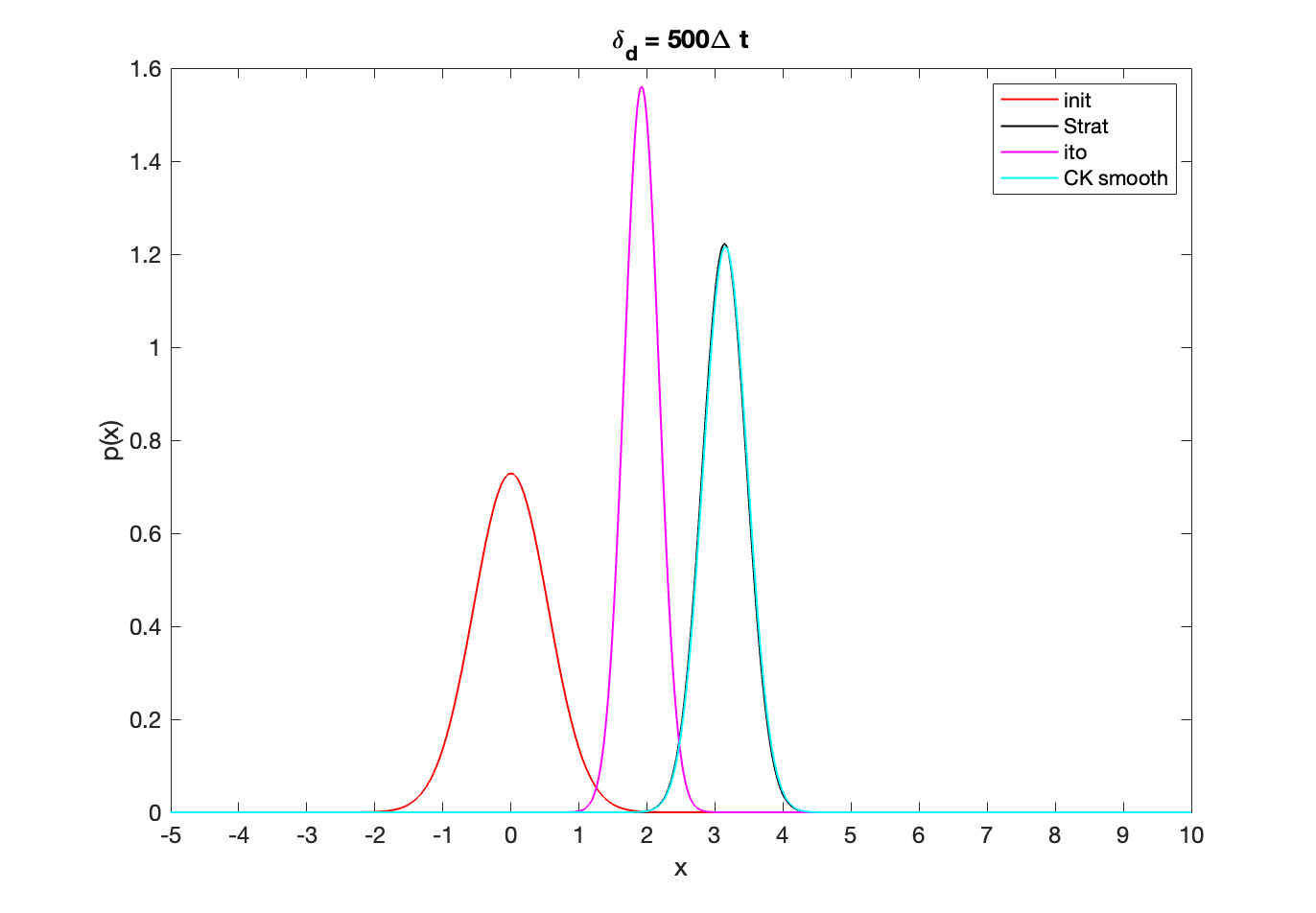
Figure 3.1: Snapshot in time for the above filtering problem with $H=2,m_{0}=0,P_{0}=0.3,x_{0}^{\ast}=5,\Xi=1$ and the smooth observations are constructed with $\delta_{d}=500\Delta t$. Clearly the Ito interpretation (pink line) is not the correct limit for the crow-kimura with smooth approximation. The correct stratonovich interpretation (black line) aligns closely with the crow-kimura with smooth obs (cyan line). Note that the stratonovich interpretation (3.10) coincides with the familar zakai equation from filtering (3.2).

The following theorem establishes the convergence of the replicator-mutator equation (in the form (3.7), as identified in Lemma 3.1) to a “generalised” form of the kushner-stratonovich equation from nonlinear filtering as $d\rightarrow\infty$. Convergence is studied via the unnormalised equations as this greatly simplifies the analysis but still yields the overall conclusion relating filtering and replicator-mutator equations due to the one to one correspondence between the unnormalised and normalised equations. Convergence to the standard filtering equations for the specific choice $r=1,s=0$; the benefits of the generalised form (ie. when $s\neq 0,r\neq 1$) will be further explored in the context of misspecified filtering in Section 4. The proof of Theorem 3.1 borrows many elements from the proof of Theorem 3.1 in [HKX02] and makes use of the representation formulae developed in [Kun82]. We extend their work to consider unbounded observation drifts $h$ (where they had assumed uniform boundedness) and to the case of multivariate rather than scalar valued observations $Z_{t}$. Due to the representation formula used here, we do not need to rely on strong convergence of piecewise smooth approximations with unbounded diffusion coefficients as developed in e.g. [Pat24] (this aspect is discussed more specifically in the proof below). The price paid is that we focus on pointwise convergence of the density functions, rather than stronger $L^{p}$ convergence, i.e. (i.e. $\mathbb{E}[\|\mu_{t}^{d}-q_{t}(x)\|_{p}^{p}]\rightarrow 0$ as $d\rightarrow\infty$ where $\|f\|_{p}^{p}:=\int_{\mathbb{R}^{d}}|f(x)|^{p}dx$. The weaker mode of convergence is still useful, particularly given that it allows us to relax restrictive assumptions on $h$ which previously did not even cover the linear-Gaussian setting. The proof of the following theorem can be found in section 5.3.

Theorem 3.1.

Assume that $g(x):\mathbb{R}^{m}\rightarrow\mathbb{R}^{m}$ and $h(x):\mathbb{R}^{m}\rightarrow\mathbb{R}^{n}$ are $C^{2}$, globally Lipschitz continuous functions satisfying linear growth conditions, i.e. there exists a constant $C>0$ such that

$$\|h(x)-h(y)\|+\|g(x)-g(y)\| \leq C\|x-y\|,\enskip x,y,\in\mathbb{R}^{m}$$

$$\|h(x)\|+\|g(x)\| \leq C(1+\|x\|),\enskip x\in\mathbb{R}^{m}$$

Let $\Sigma$ and $\Xi$ be $m\times m$ and $n\times n$ positive definite matrices respectively. Denote by $\mu_{t}^{d}(x)$ the solution to the unnormalised Crow Kimura replicator-mutator equation with time-varying fitness landscape (3.5) with $s<r,r>0$

$$\partial_{t}\mu_{t}^{d}(x) =\mathcal{L}^{\ast}\mu_{t}^{d}(x)+\mu_{t}^{d}(x)\mathbb{E}_{z\sim\mu_{t}^{d}}[f_{t}(x,z)]$$

$$=\mathcal{L}^{\ast}\mu_{t}^{d}(x)-\frac{r}{2}\|h(x)-\frac{dZ_{t}^{d}}{dt}\|_{\Xi}^{2}\mu_{t}^{d}(x)+s\left\langle h(x)-\frac{dZ_{t}^{d}}{dt},h(z)-\frac{dZ_{t}^{d}}{dt}\right\rangle_{\Xi}\mu_{t}^{d}(x)$$ (3.13)

Let $q_{t}(x)$ denote the solution of the modified Zakai equation (presented here in Ito form),

$$dq_{t}=\mathcal{L}^{\ast}q_{t}(x)-\frac{s}{2}h(x)^{\top}\Xi^{-1}h(x)q_{t}(x)+(r-s)q_{t}(x)h(x)^{\top}\Xi^{-1}dZ_{t}.$$ (3.14)

Suppose also that $q_{0}(x)=\mu_{0}^{d}(x)=f(x)$ where $f$ is a uniformly bounded $C^{\infty}$ probability density function. Then for any $T>0$,

$$\lim_{d\rightarrow\infty}\mathbb{E}\left[\sup_{0\leq t\leq T}|\mu_{t}^{d}(x)-q_{t}(x)|^{p}\right]=0,\quad\forall\enskip x\in\mathbb{R}^{m}$$ (3.15)

for $p\geq 1$ and $r,s$ additionally satisfying $r-s<\frac{2}{tC(1+\mathbb{E}^{\mathbb{Q}}[|x|^{2}])p\lambda_{\Xi}^{2}r_{1}r_{2}}$, where $r_{1},r_{2}>1$ and $1/r_{1}+1/r_{2}=1$ and $C$ depends on the linear growth constant of $h(x)$. Importantly, when $r=1,s=0$, (3.13) converges to the standard Zakai equation (3.2).

4 Replicator-mutator equations & filtering with misspecified models: the Linear-Gaussian case

Throughout this section, we use the terminology local and non-local replicator-mutator equation to refer to (3.7) with $s=0,r>0$ and $s\neq 0,r>0$, respectively. The terminology is motivated by the fact that the case $s\neq 0$ introduces a non-local term into the fitness function. Theorem 3.1 shows that $r=1,s=0$ in the crow-kimura replicator-mutator equation (3.7) coincides with the non-linear filtering equation when the system dynamics is known perfectly. In this section, we focus on the linear-Gaussian setting to demonstrate both analytically and numerically the benefits of the non-local replicator-mutator model for inference in the presence of model misspecification. Additionally, we show in Section 4.1 that the local replicator-mutator equation with $r\neq 1$ corresponds to the familiar covariance inflated ensemble Kalman-Bucy filter.

Before detailing these main insights, we first present the fundamental equations in the Linear-Gaussian setting and establish some useful findings on mean-field models corresponding to (3.7). Firstly, consider the (normalised) linear-Gaussian crow-kimura replicator-mutator equation in the limit $\delta_{d}\rightarrow 0$ as derived in Theorem 3.1. That is, consider the normalised form of (3.14) with $h(x)=Hx,\enskip g(x)=Gx,p_{0}=\mathcal{N}(x;m_{0},C_{0})$,

$$dp_{t}(x)=\mathcal{L}^{\ast}p_{t}(x)dt\,+\, (r-s)p_{t}(x)\left(-(Hx-Hm_{t})^{\top}\Xi^{-1}Hm_{t}dt+(Hx-Hm_{t})^{\top}\Xi^{-1}dZ_{t}\right)$$

$$-\frac{s}{2}p_{t}(x)\left(\|Hx-Hm_{t}\|_{\Xi}^{2}-\mathbb{E}_{p_{t}}[\|Hx-Hm_{t}\|_{\Xi}^{2}]\right)dt$$ (4.1)

noticing that this coincides with the standard Kushner equation when $r=1,s=0$. The form with $\delta_{d}>0$ is given by

$$dp_{t}(x)=\mathcal{L}^{\ast}p_{t}(x)dt+(r-s)p_{t}(x) \left(-\frac{1}{2}\left(x^{\top}H^{\top}\Xi^{-1}Hx-\mathbb{E}_{p_{t}}\left[x^{\top}H^{\top}\Xi^{-1}Hx\right]\right)+\left(Hx-Hm_{t}\right)^{\top}\Xi^{-1}\frac{dZ_{t}^{d}}{dt}\right)$$

$$-\frac{s}{2}p_{t}(x) \left(\|Hx-Hm_{t}\|_{\Xi}^{2}-\mathbb{E}_{p_{t}}[\|Hx-Hm_{t}\|_{\Xi}^{2}]\right)dt$$ (4.2)

where in the remainder of this section, we use the notation $m_{t}:=\mathbb{E}_{p_{t}}[x]$ and $C_{t}=\mathbb{E}_{p_{t}}[xx^{\top}]-\mathbb{E}_{p_{t}}[x]\mathbb{E}_{p_{t}}[x^{\top}]$ for the mean and covariance respectively. It can be shown straightforwardly that the evolution of the mean and covariance of the crow-kimura replicator-mutator equation (4.1) is given by

$$dm_{t} =Gm_{t}dt+(r-s)C_{t}H^{\top}\Xi^{-1}\left(dZ_{t}-Hm_{t}dt\right)$$ (4.3)

$$\dot{C}_{t} =GC_{t}+C_{t}G^{\top}+\Sigma-rC_{t}H^{\top}\Xi^{-1}HC_{t}$$ (4.4)

and also that the mean equation for the case $\delta_{d}>0$ (with pde given by (4.2)) is given by

$$\dot{m}_{t} =Gm_{t}+(r-s)C_{t}H^{\top}\Xi^{-1}\left(\dot{Z}_{t}^{d}-Hm_{t}\right)$$ (4.5)

and the covariance equation coinciding with (4.4). Notice in particular that while both $s$ and $r$ affect the evolution of the mean, only $r$ affects the evolution of the covariance. This aspect will be discussed further in the context of misspecified filtering in section 4.2. In the below lemma, we consider mean-field processes associated to the replicator-mutator equation. Such mean-field processes arise in interacting particle implementations of Kalman Bucy filtering (the so-called ensemble Kalman-Bucy methods, in both the stochastic form [Lee20, HM97] and deterministic forms [BR12, Tag+17]). The mean-field process helps to demonstrate that the drift term involving $s$ acts as a covariance deflation for $s<0$ and an additional inflation term for $s\in(0,r)$. The proof of the lemma can be found in section 5.4. We will utilise this characterisation to establish connections to covariance inflated Kalman-Bucy filtering specifically in section 4.1.

Lemma 4.1.

Consider the multivariate linear-Gaussian setting as described above and the following mean-field SDEs with $s<r,r>0$

$$d\bar{X}_{t}=\underbrace{G\bar{X}_{t}+\Sigma^{1/2}dW_{t}}_{\text{mutation}}\enskip -\frac{s}{2}C_{t}H^{\top}{\Xi^{-1}}(H\bar{X}_{t}-Hm_{t})dt$$

$$+\underbrace{C_{t}H^{\top}\left(\frac{1}{r-s}\Xi\right)^{-1}\left(dZ_{t}-H\bar{X}_{t}dt+\left(\frac{1}{r-s}\Xi\right)^{1/2}d\bar{W}_{t}\right)}_{\text{Stochastic Kalman Innovation}}$$ (4.6)

$$d\bar{X}_{t}=\underbrace{G\bar{X}_{t}+\Sigma^{1/2}dW_{t}}_{\text{mutation}}-sHC_{t}\Xi^{-1}\left(dZ_{t}-Hm_{t}dt\right)+\underbrace{\enskip C_{t}H^{\top}\left(\frac{1}{r-s}\Xi\right)^{-1}\left(dZ_{t}-\frac{1}{2}\left(H\bar{X}_{t}+Hm_{t}dt\right)\right)}_{\text{Deterministic Kalman Innovation}}$$ (4.7)

where $\bar{W}$ is a scalar Wiener process independent of $W,B$ and $\bar{X}_{0}\sim\mathcal{N}(x;m_{0},C_{0})$. The time evolution of the conditional density of $\bar{X}_{t}$ given $\mathcal{Z}_{t}$ for both processes (4.6) and (4.7) is given by (4.1). We may similarly define a mean-field process with smooth observations of the form

$$d\bar{X}_{t}=\underbrace{G\bar{X}_{t}+\Sigma^{1/2}dW_{t}}_{\text{mutation}}\enskip -\frac{s}{2}C_{t}H^{\top}{\Xi^{-1}}(H\bar{X}_{t}-Hm_{t})dt$$

$$+\underbrace{C_{t}H^{\top}\left(\frac{1}{r-s}\Xi\right)^{-1}\left(\frac{dZ_{t}^{d}}{dt}-H\bar{X}_{t}\right)dt+C_{t}H^{\top}\left(\frac{1}{r-s}\Xi\right)^{-1/2}d\bar{W}_{t}}_{\text{Stochastic Kalman Innovation}}$$ (4.8)

and similarly for the deterministic update version (4.7). The conditional density of (4.8) (as well as the deterministic update version) evolves according to the crow-kimura replicator-mutator equation given by (4.2).

It is well known that the Kalman-Bucy filter is the minimum variance unbiased estimator of $X_{t},\enskip t>0$. This property carries over to the crow-kimura replicator mutator equation for $s=0,r=1$ due to the pre-established equivalence to the Kalman Bucy filter. In the following result, we show that the unbiasedness property holds more generally for the replicator mutator equation (4.2), i.e. for any choice $s<r,r>0$, when the system parameters are known perfectly. Obviously both from inspection of (4.4) and also from Lemma 4.1, it is clear that the minimum variance property is destroyed unless $r=1$.

Lemma 4.2.

Unbiasedness of the non-local replicator-mutator with perfect system. Consider the signal-observation pair (1.5)-(1.6) with $g(x)=Gx,\enskip h(x)=Hx$ and Gaussian initial conditions. If $m_{0}=\mathbb{E}[X_{0}]$ then the generalised Kalman-Bucy filter with $s<r,r>0$ is unbiased, i.e. $\mathbb{E}[m_{t}]=\mathbb{E}[X_{t}],\enskip t>0$.

Proof.

Begin with the mean equation from the generalised Kalman-Bucy filter

$$m_{t} =m_{0}+\int_{0}^{t}Gm_{u}du+(r-s)\int_{0}^{t}K_{u}dZ_{u}-(r-s)\int_{0}^{t}K_{u}Hm_{u}du$$

$$=m_{0}+\int_{0}^{t}Gm_{u}du+(r-s)\int_{0}^{t}K_{u}H(X_{u}^{\ast}-m_{u})du+(r-s)\int_{0}^{t}K_{u}\Xi^{1/2}dB_{u}$$

where $K_{t}:=C_{t}H^{\top}\Xi^{-1}$ corresponds to the Kalman gain at time $t$ and we have substituted in the form of the observations in the second equality. Then

$$\mathbb{E}[m_{t}] =m_{0}+\int_{0}^{t}G\mathbb{E}[m_{u}]du+(r-s)\int_{0}^{t}K_{u}H(\mathbb{E}[X_{u}^{\ast}]-\mathbb{E}[m_{u}])du$$

Also recall that

$$\mathbb{E}[X_{t}^{\ast}]=\mathbb{E}[X_{0}^{\ast}]+\int_{0}^{t}G\mathbb{E}[X_{u}^{\ast}]du$$

then

$$\mathbb{E}[m_{t}]-\mathbb{E}[X_{t}^{\ast}]=m_{0}-\mathbb{E}[X_{0}^{\ast}]+\int_{0}^{t}(G-(r-s)K_{s}H)(\mathbb{E}[m_{s}]-\mathbb{E}[X_{s}^{\ast}])ds$$

which corresponds to an ODE of the form $\dot{y}_{t}=A_{t}y_{t}$ with $y_{t}:=\mathbb{E}[m_{t}]-\mathbb{E}[X_{t}^{\ast}]$, which has solutions $y_{t}=0,\enskip t>0$ whenever $y_{0}=0$. ∎

4.1 Replicator-mutator with $s=0,r\neq 1$ & Inflated Kalman-Bucy filtering

The mean-field processes presented in Lemma 4.1, we see that in the linear-Gaussian setting, the replicator-mutator equation with $s\neq 0$ involves both an adjustment of the observation error covariance $\Xi$ as well as the inclusion of the term $\frac{s}{2}C_{t}H^{\top}{\Xi^{-1}}(H\bar{X}_{t}-Hm_{t})$ which either acts as a mean-reversion or mean-repulsion depending on the chosen value of $s$. A similar term also appears in [WRS18] where the ensemble Kalman Bucy filter with so-called “deterministic noise” in place of the stochastic signal noise $\Sigma$ is analysed. The use of such terms has a long history in the field of ensemble Kalman filtering, where it is more widely known as covariance inflation [And07, DSH20, MH00, TMK16, BD23]. Covariance inflation is an important heuristic tool used to improve numerical stability of the ensemble Kalman filter when the number of samples is low [BMP18, BD19] and also to account for model errors.

The below lemma establishes the equivalence of the crow-kimura replicator mutator equation for both $\delta_{d}>0$ and the limiting $\delta_{d}\rightarrow 0$ case, i.e. (4.2) and (4.1) respectively, to a form of covariance inflation in the literature. The proof of the lemma can be found in section 5.5.

Lemma 4.3.

Consider the following mean field description of covariance inflated “stochastic” ensemble Kalman-Bucy filter see e.g. [BMP18, BD23],

$$d\bar{X}_{t}=G\bar{X}_{t}+\Sigma^{1/2}dW_{t}+(C_{t}+\epsilon T)H^{\top}\Xi^{-1}\left(dZ_{t}-H\bar{X}_{t}dt+\Xi^{1/2}d\bar{W}_{t}\right)$$ (4.9)

and the mean field description of covariance inflated “deterministic” ensemble Kalman-Bucy filter [BD23] with piecewise smooth observations,

$$\frac{d\bar{X}_{t}}{dt}=G\bar{X}_{t}+\Sigma^{1/2}dW_{t}+(C_{t}+\epsilon T)H^{T}\Xi^{-1}\left[\frac{dZ_{t}^{d}}{dt}-H\left(\frac{\bar{X}_{t}+m_{t}}{2}\right)\right]$$ (4.10)

where $\epsilon>0$ is a tuning parameter and $T$ is a reference matrix guiding the inflation. The corresponding evolution pde describing the conditional density $p(X_{t}|\mathcal{Z}_{t})$ for (4.9) and (4.10) is formally equivalent to (4.1) and (4.2) respectively, for the choices $T=C_{t}$, $r=1+\epsilon$ and $s=0$.

4.2 Local vs non-local replicator-mutator for misspecified model filtering

We now turn out attention to analysing the performance of the replicator-mutator equation for a filtering problem with misspecified signal dynamics. This section focuses on the $\delta_{d}\rightarrow 0$ form of the replicator-mutator, (4.1), although the conclusions of this section are expected to similarly hold for $\delta_{d}>0$. The misspecified model filtering problem is as follows. Consider the following linear-gaussian problem where the hidden state $X_{t}\in\mathbb{R}^{m}$ evolves according to

$$dX_{t}=GX_{t}dt+bdt+\Sigma^{1/2}dW_{t}$$ (4.11)

with $X_{0}\sim\mathcal{N}(m_{0},P_{0})$ and $b$ a constant vector. The hidden dynamics is known imperfectly and that the assumed model for the trait is instead

$$dX_{t}=GX_{t}dt+\Sigma^{1/2}dW_{t}$$ (4.12)

(i.e. (4.11) with $b=0$), and the observation process is as in (1.6). The replicator-mutator equation (4.2) is no longer expected to produce unbiased estimates due to the presence of the $b$ term.

Firstly, we introduce the following important variables. The tracking error at time $t$ is denoted by $\varepsilon_{t}$,

$$\varepsilon_{t}:=m_{t}-x_{t}^{\ast}$$

where $m_{t}:=\int xp_{t}(x)dx$ and $p_{t}(x)$ is the solution of (4.1) and $X_{t}^{\ast}$ the solution of (4.11), also known as the reference trajectory or true hidden state. Denote also by $P_{t}$ the error covariance matrix,

$$P_{t}:=\mathbb{E}[(\varepsilon_{t}-\mathbb{E}[\varepsilon_{t}])(\varepsilon_{t}-\mathbb{E}[\varepsilon_{t}])^{T}]$$

Note well that $P_{t}$ is distinct from $C_{t}$ which we use to denote the covariance from the replicator-mutator equation, also the covariance of the filtering equations. Recall that in the perfect knowledge Kalman Bucy filtering setting, since $\mathbb{E}[\varepsilon_{t}]=0$, we have that $C_{t}=\tilde{P}_{t}=P_{t}$. When $b\neq 0$, even a standard Kalman-Bucy filter no longer produces an unbiased estimates of the hidden state, so that $\tilde{P}_{t}\neq P_{t}$ and also, $C_{t}\neq P_{t}$. Finally, let

$$\nu_{t}:=\|\mathbb{E}[\varepsilon_{t}]\|^{2},\quad E_{t}:=\mathbb{E}[\|\varepsilon_{t}\|^{2}]$$

denote the squared expected error (or squared bias) and expected squared error (mean squared error), respectively. Notice that $\nu_{t}=Tr(\mathbb{E}[\varepsilon_{t}]\mathbb{E}[\varepsilon_{t}^{\top}])$. We also define

$$\tilde{P}_{t}:=\mathbb{E}[\varepsilon_{t}\varepsilon_{t}^{\top}]$$ (4.13)

and notice that $Tr(\tilde{P}_{t})=E_{t}$. Recall that when $b=0$, we have that $\mathbb{E}[\varepsilon_{t}]=0$ for all $t$ from lemma 4.2, so that $P_{t}=\tilde{P}_{t}$. Since our focus is on the case $b\neq 0$, it is necessary to further study $\tilde{P}_{t}$ in its own right. Additionally, since $\tilde{P}_{t}=P_{t}+\mathbb{E}[\varepsilon_{t}]\mathbb{E}[\varepsilon_{t}^{\top}]$ the following bias-variance decomposition holds

$$\underbrace{E_{t}}_{=\text{m.s.e}}=\underbrace{Tr(P_{t})}_{=\text{total error var.}}+\underbrace{\nu_{t}}_{=\text{squared bias}}$$

Finally, we use the shorthand notation

$$K_{t}:=C_{t}H^{\top}\Xi^{-1}$$

which for the case $r=1$ coincides with the familiar Kalman Gain from the Kalman-Bucy filter. The following lemma characterises the time evolution of bias, variance and mean squared error. As expected, the error variance $P_{t}$ evolves independently of the unknown term $b$. The proof of the lemma can be found in section 5.6

Lemma 4.4.

Assume the system properties described by (4.11) for the true hidden state, (4.12) for the assumed hidden state and (1.6) for the observation model. Given $\Xi^{-1/2}H$ an invertible matrix and $r,s$ such that $r<s,r>0$, we have the following evolution equations for the error covariance $P_{t}$ and expected squared error $\tilde{P}_{t}$,

$$\frac{dP_{t}}{dt} =(G-(r-s)K_{t}H)P_{t}+P_{t}(G-(r-s)K_{t}H)^{\top}+\Sigma dt+(r-s)^{2}K_{t}\Xi K_{t}^{\top}$$ (4.14)

$$\frac{d\tilde{P}_{t}}{dt} =(G-(r-s)K_{t}H)\tilde{P}_{t}+\tilde{P}_{t}(G-(r-s)K_{t}H)^{\top}+\Sigma+(r-s)^{2}K_{t}\Xi K_{t}^{\top}-\mathbb{E}[\varepsilon_{t}]b^{\top}-b\mathbb{E}[\varepsilon_{t}^{\top}]$$ (4.15)

For the special case $s=0,r=1$, it holds that $P_{t}=C_{t},\enskip\forall\enskip t>0$ if $P_{0}=C_{0}$ where $C_{t}$ is the solution of the covariance equation of the replicator-mutator.

Furthermore,for any p.d. $C_{0}$, the evolution of the mean squared error $E_{t}$ satisfies the following inequality

$$\frac{dE_{t}}{dt}\leq 2\|(A_{t}(r,s)\|_{F}E_{t}-2Tr(\mathbb{E}[\varepsilon_{t}]b^{\top})+Tr(\Sigma)+(r-s)^{2}\lambda_{max}(H^{\top}\Xi^{-1}H)\|C_{t}\|_{F}$$ (4.16)

where $A_{t}(r,s):=G-(r-s)K_{t}H$.

To obtain further insights on optimal choices of $r,s$, we consider a simplified setting where $C_{0}=C_{\infty}$ (i.e. where the covariance is initialised at the steady state covariance matrix in (4.4)). This setting is still rich enough to provide insights on the role of $r,s$ in the non-local replicator-mutator, particularly as we are primarily interested in the time asymptotic behaviour of mean squared error. Whilst the calculations in the previous section are applicable in the multivariate setting, from now on we focus purely on the fully scalar case, and leave the multivariate setting to future work. For the remainder of the section, we use $\tilde{P}_{t}$ to refer to the mean square error. The following lemma gives explicit representations of the time asymptotic squared bias $\nu_{\infty}$ and mean squared error $E_{\infty}$ where $E_{t}=\tilde{P}_{t}$ in the scalar case. The proof of the lemma can be found in section 5.7.

Lemma 4.5.

Steady state Bias-Variance. Consider the scalar setting where $m=n=1$. Assume $\mathbb{E}[\varepsilon_{0}=0]$ and $C_{0}=C_{\infty}$ where $C_{\infty}$ satisfies

$$0=GC_{\infty}+C_{\infty}G^{\top}+\Sigma-rC_{\infty}H^{\top}\Xi^{-1}HC_{\infty}$$ (4.17)

Suppose $r,s$ are specified such that $A_{\infty}<0$. Then as $t\rightarrow\infty$, $\nu_{t}\rightarrow\nu_{\infty}$ and $\tilde{P}_{t}\rightarrow\tilde{P}_{\infty}$ where

$$\nu_{\infty} =\left(\frac{b}{A_{\infty}(r,s)}\right)^{2}$$ (4.18)

$$\tilde{P}_{\infty} =-\frac{1}{2}\left(\Sigma+\left(\frac{G-A_{\infty}(s,r)}{H}\right)^{2}\Xi\right)\frac{1}{A_{\infty}(s,r)}+\left(\frac{b}{A_{\infty}(s,r)}\right)^{2}$$ (4.19)

and

$$A_{\infty}(s,r) =\frac{s}{r}G+\frac{(r-s)}{r}A_{\infty}(0,r)$$ (4.20)

$$A_{\infty}(0,r) =-\sqrt{G^{2}+rH^{2}\Xi^{-1}\Sigma}$$ (4.21)

We are now ready to characterise the optimal $r,s$ values that minimise mean square error. Recall that the minimal conditions on $s,r$ are that $r>0$ and $s<r$. The below lemma establishes a range of allowable values of $s$ in terms of $r$ which guarantee the existence of a stable mean squared error value, $\tilde{P}_{\infty}$. Importantly, the lemma shows that there is not one unique pair $(r,s)$ that minimises the asymptotic mean square error for a given system, but rather infinitely many pairs satisfying (4.26). These estimates hold true regardless of the stability characteristics of the hidden state and observation dynamics. Additionally, we demonstrate that for $s\in(s^{l},s^{u})$ where $s^{l},s^{u}$ are as defined in the below lemma, there exists two possible $r$ values for a given $s$ that will yield the minimal asymptotic mean square error. This is particularly beneficial in terms of allowing for a realistic $C_{\infty}$, as will be explored further in Lemma 4.7. The proof of lemma 4.6 can be found in section 5.8.

Lemma 4.6.

Optimal $r,s$ minimising m.s.e. Adopt the same conditions as in Lemma 4.5. Define,

$$p :=-(H^{2}\Xi^{-1}\Sigma+G^{2}),\quad q:=4b^{2}H^{2}\Xi^{-1}$$ (4.22)

$$\tau :=\frac{q^{2}}{4}+\frac{p^{3}}{27}$$ (4.23)

Suppose that $G,H,\Sigma,\Xi,b$ are such that $\tau\neq 0$. Finally, define $A_{\infty}^{\star}$ depending on whether $\tau<0$ or $\tau>$, as

$$A_{\infty}^{\ast}:=\begin{cases}\left(-\frac{q}{2}+\sqrt{\tau}\right)^{1/3}+\left(-\frac{q}{2}-\sqrt{\tau}\right)^{1/3},\enskip\tau>0\\ 2\,\sqrt{-\frac{p}{3}}\,\cos\left[\,\frac{1}{3}\cos^{-1}\left(\frac{3q}{2p}\sqrt{\frac{-3}{p}}\,\right)-\frac{4\pi}{3}\,\right],\enskip\tau<0\end{cases}$$ (4.24)

Then the admissible values of $s$ for any $r>0$ satisfy

$$s^{l}:=-\frac{(G+A_{\infty}^{\ast})^{2}}{4H^{2}\Xi^{-1}\Sigma}<s<\min\left(r,\frac{\sqrt{G^{2}+rH^{2}\Xi^{-1}\Sigma}}{G+\sqrt{G^{2}+rH^{2}\Xi^{-1}\Sigma}}r\right)$$ (4.25)

where the upper bound guarantees the existence of $\tilde{P}_{\infty}$. The optimal $s$ for any given $r>0$ is given by

$$s^{\text{opt}}=\frac{r(A_{\infty}^{\ast}+\sqrt{G^{2}+rH^{2}\Xi^{-1}\Sigma})}{G+\sqrt{G^{2}+rH^{2}\Xi^{-1}\Sigma}}$$ (4.26)

Alternatively, for any $s\in\left(s^{l},s^{u}\right)$ where $s^{u}:=\frac{G^{2}+(A_{\infty}^{\ast}-G)|G|-GA_{\infty}^{\ast}}{H}$, there are two possible values of $r$ optimising mse, given by

$$r^{\text{opt}}=\frac{1}{4H^{2}\Xi^{-1}\Sigma}\left(G-A_{\infty}^{\ast}\pm\sqrt{(G-A_{\infty}^{\ast})^{2}+4(GA_{\infty}^{\ast}+sH^{2}\Xi^{-1}\Sigma)}\right)^{2}-\frac{G^{2}}{H^{2}\Xi^{-1}\Sigma}$$ (4.27)

and for any $s^{u}<s<\min\left(r,\frac{\sqrt{G^{2}+rH^{2}\Xi^{-1}\Sigma}}{G+\sqrt{G^{2}+rH^{2}\Xi^{-1}\Sigma}}r\right)$, there is a unique optimal $r$, given by

$$r^{\text{opt}}=\frac{1}{4H^{2}\Xi^{-1}\Sigma}\left(G-A_{\infty}^{\ast}+\sqrt{(G-A_{\infty}^{\ast})^{2}+4(GA_{\infty}^{\ast}+sH^{2}\Xi^{-1}\Sigma)}\right)^{2}-\frac{G^{2}}{H^{2}\Xi^{-1}\Sigma}$$ (4.28)

Importantly, the above lemma shows that there are infinitely many $(s,r)$ satisfying (4.26), $r>0,s<r$ and $A_{\infty}<0$, and these will all yield the minimum mean squared error $\tilde{P}_{\infty}$ as $t\rightarrow\infty$, as well as the same error variance $P_{\infty}$ and squared bias $\nu_{\infty}$ (since each of these terms depend only on $A_{\infty}$). However, $C_{\infty}$ will clearly be different, due to the dependence on the chosen $r$ value (see (5.20)). As can be seen in the next lemma (and also in section 4.3), larger values of $r$ lead to smaller $C_{\infty}$. From an inference perspective, smaller $C_{\infty}$ indicates greater confidence in the estimator, which can be problematic especially when $C_{\infty}$ is smaller than the minimum covariance achievable in the perfect model setting. To analyse this phenomenon further, define

$$\hat{C}_{\infty}:=\frac{G+\sqrt{G^{2}+H^{2}\Xi^{-1}\Sigma}}{H^{2}\Xi^{-1}}$$ (4.29)

which is the steady state covariance coinciding with the Kalman-Bucy filter (the optimal filter) in the case of perfect knowledge, (i.e. when $r=1,s=0,b=0$). Any choice of $r$ for which $C_{\infty}<\hat{C}_{\infty}$ should be avoided when there is model misspecification, as we cannot expect to be more confident than when we have no misspecification. Recall that in the perfect knowledge setting, we have that $\tilde{P}_{\infty}=\hat{C}_{\infty}$, in other words, the asymptotic covariance from the Kalman-Bucy filter coincides with the mean squared error. The following lemma establishes a relationship between $r,s$ that ensures the specific pair satisfies $C_{\infty}=\tilde{P}_{\infty}$ in the misspecified model setting where $b\neq 0$. This highlights that the non-local replicator-mutator equation, unlike the regular inflated ensemble Kalman method, is capable of simultaneously minimise mean squared error and providing realistic uncertainty estimates through $C_{\infty}$. In particular, (4.31) in the below lemma demonstrates that the standard inflated ensemble Kalman method requires $r>1$ to minimise mse. It will be demonstrated numerically in section 4.3 that this often coincides with an under-representation of the uncertainty (i.e. $\frac{C_{\infty}(r_{0}^{\text{opt}})}{\hat{C}_{\infty}}<<1$). The last claim of the below lemma takes a step towards this claim analytically, by demonstrating that $\frac{C_{\infty}(r)}{\hat{C}_{\infty}}\rightarrow 0$ as $r\rightarrow\infty$ whenever $s=0$ (see (4.32)). The proof can be found in section 5.9.

Lemma 4.7.

Adopt the same conditions as in Lemma 4.5. Then the following holds,

1. The optimal $(r,s)$ such that $\tilde{P}_{\infty}=C_{\infty}$ satisfies (4.26) and

   $$r^{\text{opt}}-s^{\text{opt}}=\frac{(A_{\infty}^{\ast})^{2}(G-A_{\infty}^{\ast})}{-0.5A_{\infty}^{\ast}\left(H^{2}\Xi^{-1}\Sigma+(G-A_{\infty}^{\ast})^{2}\right)+b^{2}H^{2}\Xi^{-1}}$$ (4.30)

   where $A_{\infty}^{\ast}$ is given by (4.24).

2. For the case $\tau>0$, choosing $s=0$ corresponds to

   $$r_{0}^{\text{opt}}>\frac{2(G^{2}+H^{2}\Xi^{-1}\Sigma)}{H^{2}\Xi^{-1}\Sigma}>1$$ (4.31)

   independently of the unknown $b$ and for any $G,H\neq 0$ and $\Xi,\Sigma>0$. Since $r_{0}^{\text{opt}}>1$, this also means that

   $$\frac{C_{\infty}(r_{0}^{\text{opt}})}{\hat{C}_{\infty}}<\frac{1}{\sqrt{r_{0}^{\text{opt}}}}\left(\frac{2|G|+\sqrt{H^{2}\Xi^{-1}\Sigma}}{(G+\sqrt{G^{2}+H^{2}\Xi^{-1}\Sigma})}\right)$$ (4.32)

4.3 Numerical experiments

The following experiment aims to provide further insights on the role of $s,r$ in (3.13) with fitness landscape $f_{t}(x,z)$ given by (3.5) for the misspecified model setting from the previous section (which we repeat here for convenience). Although the analysis in the previous section has been done for the limiting case $\delta_{d}\rightarrow 0$, here we focus on the practically relevant discrete case and show that much of the analysis holds for $\delta_{d}$ small enough. That is, consider a partition of the time interval $[0,T]$, $0<t_{1}<t_{2}\dots<t_{d}=T$ with time-step $t_{i+1}-t_{i}=\delta_{d}$. Synthetic observations of the form

$$\frac{dZ_{t}^{d}}{dt}=Hx_{t_{i}}^{\ast}(\omega)+\Xi^{1/2}\frac{dB_{t}^{d}}{dt},\quad t\in[t_{i},t_{i+1})$$ (4.33)

(as in (3.4)) are constructed, where $x_{t}^{\ast}(\omega)$ is a solution for a realisation $\omega$ at time $t$ of

$$dX_{t}=GX_{t}dt+bdt+\Sigma^{1/2}dW_{t}$$ (4.34)

with $X_{0}\sim\mathcal{N}(m_{0},P_{0})$. The process in (4.11) describes the evolution of the actual optimal trait and $\frac{dZ_{t}^{d}}{dt}$ corresponds to noisy observations of it. Suppose the assumed model for the trait is instead

$$dX_{t}=GX_{t}dt+\Sigma^{1/2}dW_{t}$$ (4.35)

(i.e. (4.11) with $b=0$), so that the corresponding replicator-mutator equation takes the form

$$\partial p_{t}(x)=-G\nabla\cdot p_{t}(x)+\frac{1}{2}\nabla\cdot(\Sigma\nabla p_{t}(x))+p_{t}(x)\left(\mathbb{E}_{z\sim p_{t}}[f_{t}(x,z)]-\mathbb{E}_{x,z\sim p_{t}}[f_{t}(x,z)]\right)$$ (4.36)

with $f_{t}(x,z)$ given by (3.5). The remainder of this section will focus on the following experimental settings, which have been randomly generated.

Parameter	System 1 $(\tau>0)$	System 2 $(\tau<0)$
$G$	0.5	2.5
$H$	8.5	2.9
$\Sigma$	0.8	18
$\Xi$	6.3	26
$b$	9.9	1.2

Note that throughout, we assume $C_{0}=C_{\infty}$ given by (5.20). The settings in System 1 and 2 correspond to the case where $\tau>0$ (i.e. (5.23) has one real root) and $\tau<0$ (i.e. (5.23) has three real roots), respectively. Notice that in both systems, the hidden state evolves according to unstable dynamics and the crow- Kimura replicator mutator is capable of tracking an unstable signal as $A_{t}<0$. We restrict the time domain to one where machine precision doesn’t become an issue. We adopt $\delta_{d}=10^{-3}$ and use a simulation time step of $10^{-4}$ to construct the true hidden state as well as to discretise the mean and covariance equation (4.3) and (4.4) using forward euler. We have the following main insights.

Verification of lemma 4.6.

Figures 4.2 and 4.2 show the empirical estimate of the asymptotic mean square error $\tilde{P}_{\infty}$ for different $(r,s)$ pairs for system 1 and 2 respectively. The empirical mse at time $t$, $\mathcal{E}_{t}$, was calculated as

$$\mathcal{E}_{t}=\frac{1}{N_{s}}\sum_{j=1}^{N_{s}}\left(m_{t}^{j}-x_{t}^{\ast}\right)^{2}$$ (4.37)

where $x_{t}^{\ast}$ is a single fixed realisation of (4.11) and $m_{t}^{j}$ is a solution of (4.5) with $C_{0}=C_{\infty}$ and the index $j$ referring to a single realisation of the smooth observation path $Z_{t}^{d}$. We used a total of with $N_{s}=5000$. Figures 4.2 and 4.2 show that in both experiments, the analytic expressions in (4.26) and for the smallest optimal $s$ value, $s^{l}$ as given in (4.25) matches quite closely. Notice also that in system 1, Figure 4.2 we see that there are two optimal $r$ values for every $s^{l}<s<0$, since 0 is the approx value of $s^{u}$ in this case, as also described in Lemma 4.6. Conversely, for system 2 this only happens for $0<r<1.09$ as $s^{l}=-0.047$ is fairly close to zero, and is barely visible in the figure. Nevertheless, for system 1 in particular it is apparent that choosing $s<0$ allows to choose smaller $r$ values that can simultaneously reduce mean square error and provide a realistic representation of uncertainty via $C_{\infty}$.

Figure 4.1: Plot of MSE for various $s$ vs $r$ values for System 1. The (optimal in terms of mse) values are indicated by the red line, calculated using (4.26). Colourbar shows corresponding values of the asymptotic MSE $\tilde{P}_{\infty}$. The dashed red line on the left plot shows the theoretical expression for $s^{l}$ as in (4.25)

.

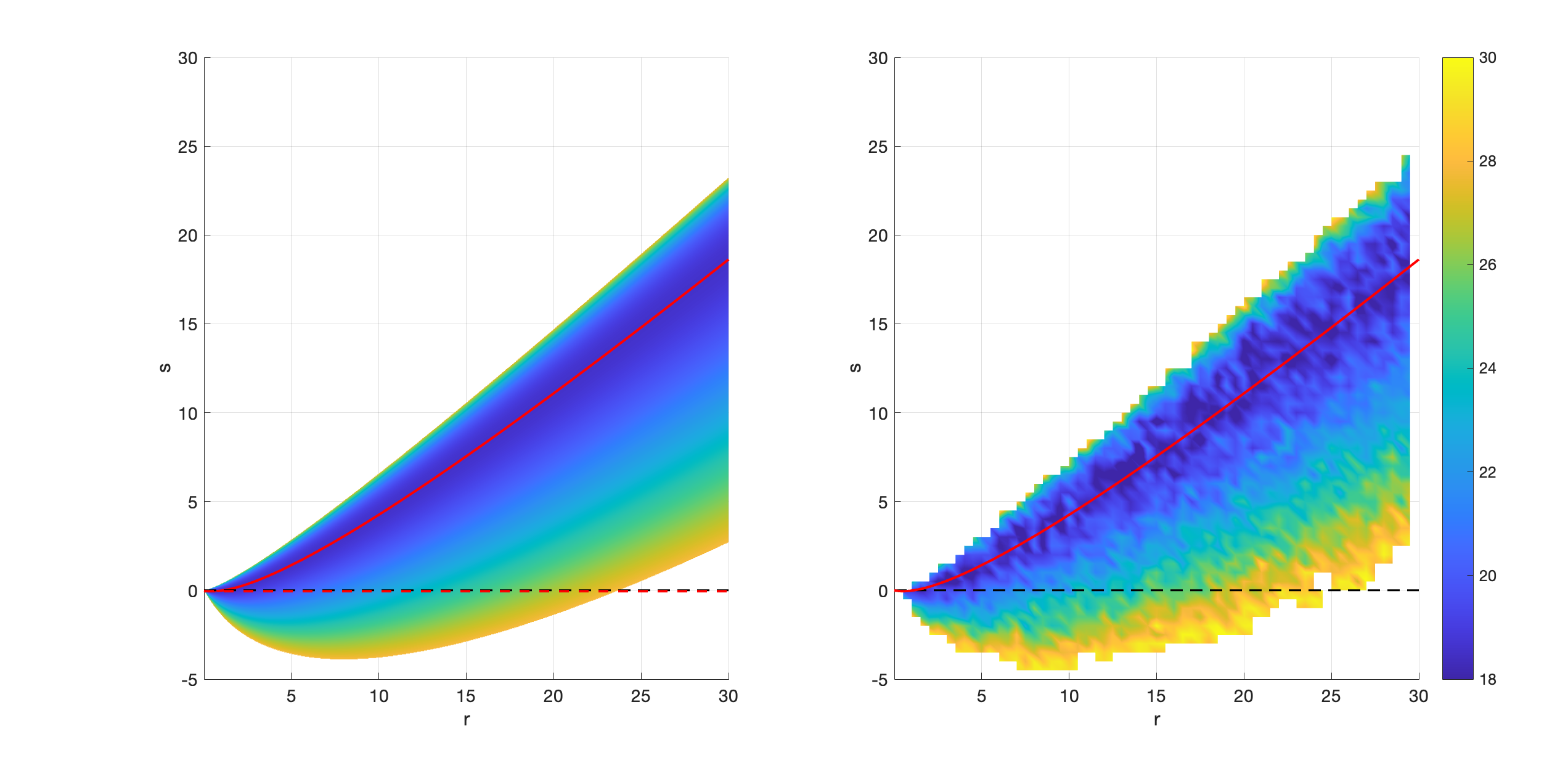
Figure 4.2: Plot of MSE for various s vs r values for System 2. The (optimal in terms of mse) values are indicated by the red line, calculated using (4.26). Colourbar shows corresponding values of the asymptotic MSE $\tilde{P}_{\infty}$.

Uncertainty quantification with $C_{\infty}$.

Recall that we may further constrain the optimal $(r,s)$ values by enforcing the requirement that $C_{\infty}=\tilde{P}_{\infty}$. This allows us to construct a filter for which the covariance of the estimate coincides with the actual mean squared error, as one obtains from the regular Kalman-Bucy filter in the perfect model setting. Figure 4.4 shows the variation in asymptotic covariance $C_{\infty}$ for different $r$ values, obtained from (5.20). Notice here that in the regular inflation case $s=0$, the asymptotic covariance for the corresponding optimal $r_{0}^{\text{opt}}$ is ($\tilde{C}_{\infty}=0.05$), which is considerably smaller than the covariance in the perfect model setting ($\tilde{C}_{\infty}=0.31$), indicating overconfidence in the estimation. The non-local replicator mutator on the other hand allows to obtain estimates that simultaneously minimise mse and provide a realistic representation of uncertainty. More specifically, the choice $r=0.13$ (which coincides with $s^{\text{opt}}=-1.18$ gives a $C_{\infty}$ which coincides with the MSE, so that the covariance produced by the estimation algorithm provides us with useful uncertainty quantification. In particular, it represents an increase in uncertainty over the perfect knowledge case (pink line), which should be reflected given the unknown bias in the system. Figure 4.3 also verifies the relation between $r,s$ in (4.30) given in Lemma 4.7 (see cyan line). This extra criterion can be used to identify a single optimal $(r,s)$ pair (as the cyan line intersects with the blue line at only one point, see Figure 4.3). In particular, for system 1, choosing $s^{\text{opt}}=-1.18$ can also yield a corresponding $r^{\text{opt}}=27.9$ (see left plot in Figure 4.3). This $r$ value is close to that of the $s=0$ case (regular covariance inflation), where it was shown that one obtains over-confident estimates. Similar conclusions can be drawn for System 2, but the optimal $(r,s)$ such that $C_{\infty}=\tilde{P}_{\infty}^{\text{opt}}$ is $s^{\text{opt}}=-0.012,r^{\text{opt}}=0.99$, is not significantly different from the regular inflation case where $s=0,r^{\text{opt}}=1.09$. Similar to System 1, the other possible choice for $r$ when $s=-0.012$, $r=0.07$, coincides with an overestimation of uncertainty ($C_{\infty}\approx 210$ vs $\tilde{P}_{\infty}=18$). We leave a study of specific system characteristics that would benefit most from the non-local replicator-mutator approach to future work.

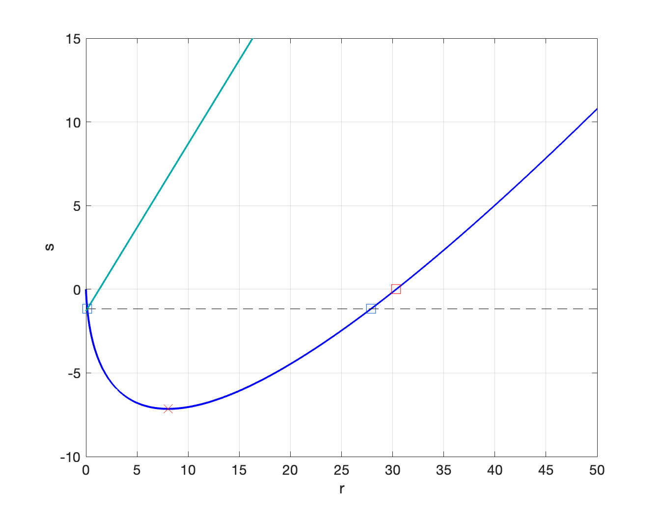
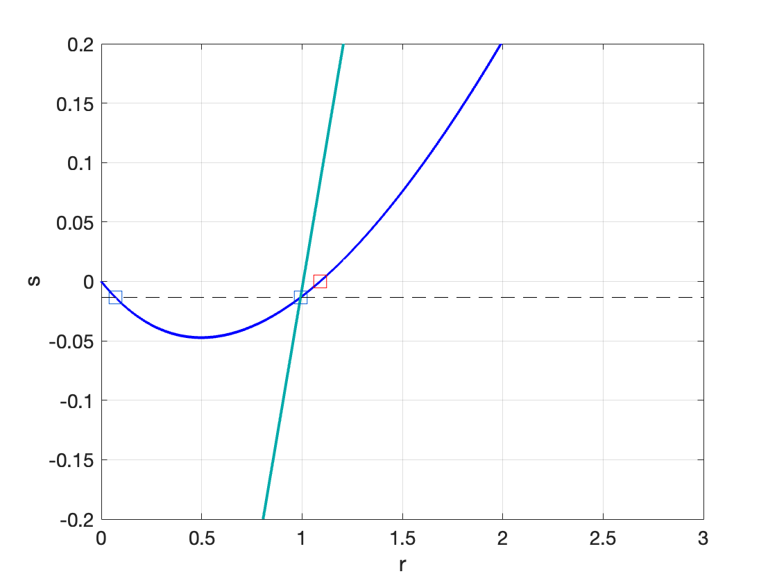
Figure 4.3: Plot of optimal $(r,s)$ values for System 1 (left plot) and System 2 (right plot). The blue line indicates the $(r,s)$ pairs minimising mse only, obtained from (4.26) and the cyan line indicates the $(r,s)$ pairs such that $C_{\infty}=\tilde{P}_{\infty}$, obtained from (4.30). The point of intersection of the two lines indicates the $(r,s)$ pair that achieves both. The red square indicates the optimal $r$ value corresponding to the regular covariance inflation case $(s=0)$. The blue squares indicate the possible $r$ values corresponding to the optimal $s$ in terms of both mse and $C_{\infty}=\tilde{P}_{\infty}$. In System 1, the standard inflation leads to overconfident estimates ($C_{\infty}$ too small), whereas in System 2, it is not so far off from the optimal choice of $s=-0.0135,r=0.99$.

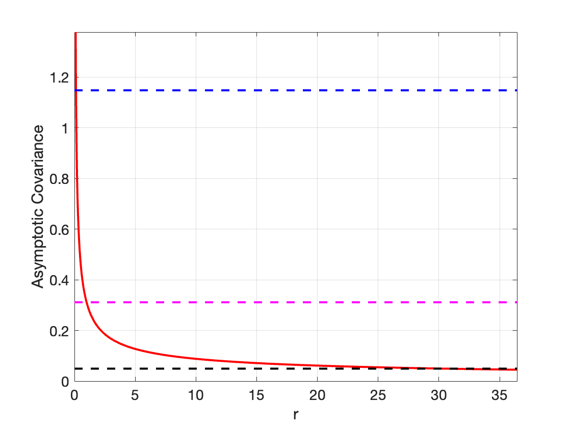
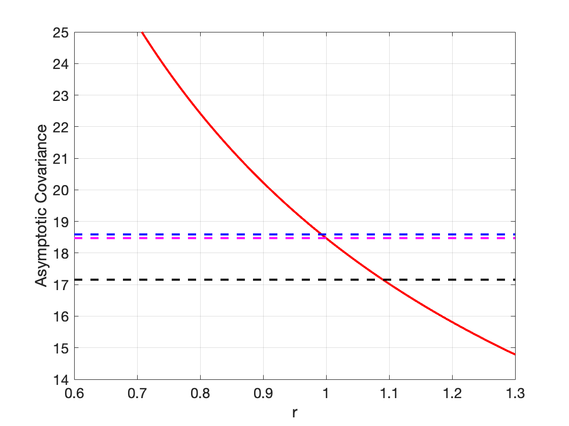
Figure 4.4: Demonstration of more realistic/representative covariances that can be obtained with the non-local replicator mutator, i.e. with $s\neq 0$. Left plot indicates system 1, right plot indicates system 2. The red solid line indicates $C_{\infty}$ for $r$ using (5.20). The blue horizontal dashed line indicates the value of $\tilde{P}_{\infty}^{\text{opt}}$, the minimum mean squared error, the pink horizontal dashed line indicates $C_{\infty}$ for $r=1$ (i.e. $\hat{C}_{\infty}$ as defined in (4.29) , the covariance in the perfect model case). Finally, the black dashed line indicates $C_{\infty}$ for $(s=0,r^{\text{opt}})$, i.e. the regular inflation case.

5 Proofs

5.1 Proof of Lemma 2.1

Proof.

We now restrict $\mathcal{P}$ to be the set of smooth probability density functions

$$\mathcal{P}(\mathbb{R}^{d}):=\Bigl{\{}p\in C^{\infty}(\mathbb{R}^{d}):\int p(x)dx=1,\enskip p\geq 0\Bigr{\}}$$

whose tangent space is given by

$$T_{p}\mathcal{P}(\mathbb{R}^{d})=\Bigl{\{}\sigma\in C^{\infty}(\mathbb{R}^{d}):\int\sigma(x)dx=0\Bigr{\}}$$

We start by computing the Fréchet derivative of (2.8) at $p$: Set $\varepsilon>0$ and $q\in\mathcal{M}$.

$$\frac{\mathcal{F}(q+\varepsilon\tilde{q})-\mathcal{F}(q)}{\varepsilon} =-\iint f(x,z)\frac{(q(x)+\varepsilon\tilde{q}(x))(q(z)+\varepsilon\tilde{q}(z))-q(x)q(z)}{2\varepsilon}\,\mathrm{d}z\,\mathrm{d}x$$

$$=-\frac{1}{2}\iint f(x,z)\left[q(x)\tilde{q}(z)+q(z)\tilde{q}(x)+\varepsilon\tilde{q}(x)\tilde{q}(z)\right]\,\mathrm{d}z\,\mathrm{d}x.$$

This means that, because $f$ is symmetric in its components,

$$D_{q}\mathcal{F}[\tilde{q}] =-\iint f(x,z)q(z)\tilde{q}(x)\,\mathrm{d}z\,\mathrm{d}x=-\int\pi_{q}(x)\tilde{q}(x)\,\mathrm{d}x=-\langle\pi_{q},\tilde{q}\rangle$$

which shows that

$$\mathcal{F}^{\prime}(p)=-\pi_{p}$$

(this is to be understood as a linear operator). For the dissipation mechanism, consider the Fisher-Rao metric defined as

$$g_{p}^{FR}(\sigma_{1},\sigma_{2}) =\int\frac{\sigma_{1}}{p(x)}\frac{\sigma_{2}}{p(x)}\,\mathrm{d}p(x)=\int\sigma_{1}\frac{\sigma_{2}}{p(x)}\,\mathrm{d}x$$

$$\equiv\int\sigma_{1}\frac{\sigma_{2}}{p(x)}\,\mathrm{d}x-\int\sigma_{1}dx\cdot\int\sigma_{2}\,\mathrm{d}x$$

since $\sigma\in T_{p}\mathcal{P}$ satisfies $\int\sigma dx=0$. Its corresponding isomorphism/dual action $\mathcal{G}^{FR}(p):T_{p}\mathcal{P}\rightarrow T_{p}^{\ast}\mathcal{P}$ is given (by inspection) as

$$\mathcal{G}^{FR}(p)\sigma=\frac{\sigma}{p}-\int\sigma dx$$ (5.1)

The inverse mapping is given by

$$\mathcal{G}^{FR}(p)^{-1}\Phi=\left(\Phi-\int\Phi\,p(x)dx\right)p.$$ (5.2)

Straightforwardly, we have

$$-\mathcal{G}^{FR}(p)^{-1}\mathcal{F}^{\prime}(p)=\left(\pi_{p}(x)-\int\pi_{p}(x)p(x)dx\right)p(x)$$

which yields the right-hand side of the replicator equation.

∎

5.2 Proof of Lemma 3.1

Proof.

The result follows from a simple re-arrangement of (3.13). Throughout, we use the shorthand notation $y_{t}:=\frac{dZ_{t}^{d}}{dt}$ and recall that $\|v(x)\|_{\Xi}^{2}:=v(x)^{\top}\Xi^{-1}v(x)$ for vector valued functions $v(x):\mathbb{R}^{d}\rightarrow\mathbb{R}^{d}$. Firstly,

$$\mathbb{E}_{z\sim\rho_{t}}[f_{t}(x,z)]-\mathbb{E}_{\rho_{t}}[f_{t}] =\int\left(-\frac{r}{2}\|h(x)-y_{t}\|_{\Xi}^{2}+s\langle h(x)-y_{t},h(z)-y_{t}\rangle_{\Xi}\right)\rho_{t}(z)dz$$

$$-\int\int\left(-\frac{r}{2}\|h(x)-y_{t}\|_{\Xi}^{2}+s\langle h(x)-y_{t},h(z)-y_{t}\rangle_{\Xi}\right)\rho_{t}(x)\rho_{t}(z)dxdz$$

$$=-\frac{r}{2}\left(\|h(x)-y_{t}\|_{\Xi}^{2}-\mathbb{E}_{\rho_{t}}[\|h-y_{t}\|_{\Xi}^{2}]\right)+s\langle h(x)-y_{t},\mathbb{E}_{\rho_{t}}[h]-y_{t}\rangle_{\Xi}-s\|\mathbb{E}_{\rho_{t}}[h]-y_{t}\|_{\Xi}^{2}$$

$$=:I_{1}(x)+sI_{2}(x)+sI_{3}(x)$$

For the first term, we have

$$I_{1}(x) =-\frac{r}{2}\left(h(x)^{\top}\Xi^{-1}h(x)-h(x)^{\top}\Xi^{-1}y_{t}-y_{t}^{\top}\Xi^{-1}h(x)-\mathbb{E}_{\rho_{t}}[h^{\top}\Xi^{-1}h]+\mathbb{E}_{\rho_{t}}[h^{\top}]\Xi^{-1}y_{t}+y_{t}^{\top}\Xi^{-1}\mathbb{E}_{\rho_{t}}[h]\right)$$

$$=-\frac{r}{2}\left(h(x)^{\top}\Xi^{-1}h(x)-\mathbb{E}_{\rho_{t}}[h(x)^{\top}\Xi^{-1}h(x)]\right)+r\left(h(x)-\mathbb{E}_{\rho_{t}}[h]\right)^{\top}\Xi^{-1}y_{t}$$

For the remaining terms, we have that

$$I_{2}(x)+I_{3}(x) =\langle h-\mathbb{E}_{\rho_{t}}[h],\mathbb{E}_{\rho_{t}}[h]-y_{t}\rangle_{\Xi}$$

$$=-\frac{1}{2}\|h-\mathbb{E}_{\rho_{t}}[h]\|_{\Xi}^{2}-\frac{1}{2}\mathbb{E}_{\rho_{t}}[h^{\top}]\Xi^{-1}\mathbb{E}_{\rho_{t}}[h]+\frac{1}{2}h^{T}\Xi^{-1}h-\frac{1}{2}\mathbb{E}_{\rho_{t}}[h^{T}\Xi^{-1}h]$$

$$+\frac{1}{2}\mathbb{E}_{\rho_{t}}[h^{T}\Xi^{-1}h]-(h-\mathbb{E}_{\rho_{t}}[h])^{T}\Xi^{-1}y_{t}$$

$$=-\frac{1}{2}\|h-\mathbb{E}_{\rho_{t}}[h]\|_{\Xi}^{2}+\frac{1}{2}\left(\mathbb{E}_{\rho_{t}}[h^{T}\Xi^{-1}h]-\mathbb{E}_{\rho_{t}}[h^{\top}]\Xi^{-1}\mathbb{E}_{\rho_{t}}[h]\right)$$

$$+\frac{1}{2}\left(h^{T}\Xi^{-1}h-\mathbb{E}_{\rho_{t}}[h^{T}\Xi^{-1}h]\right)-(h-\mathbb{E}_{\rho_{t}}[h])^{T}\Xi^{-1}y_{t}.$$

Combining yields

$$I_{1}(x)+sI_{2}(x)+sI_{3}(x) =-\frac{1}{2}(r-s)\left(h(x)^{\top}\Xi^{-1}h(x)-\mathbb{E}_{\rho_{t}}[h(x)^{\top}\Xi^{-1}h(x)]\right)+(r-s)\left(h(x)-\mathbb{E}_{\rho_{t}}[h]\right)^{\top}\Xi^{-1}y_{t}$$

$$-\frac{s}{2}\|h-\mathbb{E}_{\rho_{t}}[h]\|_{\Xi}^{2}+\frac{s}{2}\left(\mathbb{E}_{\rho_{t}}[h^{T}\Xi^{-1}h]-\mathbb{E}_{\rho_{t}}[h^{\top}]\Xi^{-1}\mathbb{E}_{\rho_{t}}[h]\right).$$

Substituting the above into (3.13) yields (3.7).

∎

5.3 Proof of Theorem 3.1

Proof.

Start with the reformulation of (3.13) as derived in Lemma 3.1, (repeating here for convenience)

$$\partial_{t}\mu_{t}^{d}(x)=\mathcal{L}^{\ast}\mu_{t}^{d}(x)+\left(-\frac{r}{2}h(x)^{\top}\Xi^{-1}h(x)+(r-s)h(x)^{\top}\Xi^{-1}\frac{dZ_{t}^{d}}{dt}\right)\mu_{t}^{d}(x)$$ (5.3)

and the Stratonovich form of (3.14),

$$dq_{t}=\mathcal{L}^{\ast}q_{t}(x)dt-\frac{r}{2}h(x)^{\top}\Xi^{-1}h(x)q_{t}(x)dt+(r-s)q_{t}(x)h(x)^{\top}\Xi^{-1}\circ dZ_{t}.$$ (5.4)

We proceed with the following steps. The proof below is inspired by the proof of Theorem 3.1 in [HKX02] except for the following important extensions: 1) we no longer assume $h$ is uniformly bounded; 2) $h$ is no longer a scalar valued function but may be vector valued; 3) we make use of the forward stochastic Feynman-Kac style representation formula in [Kun82] rather than the backward formula. Existence and uniqueness of density valued solutions to the zakai equation in $L^{2}(\mathbb{R}^{m})$ with $g,h$ unbounded has been studied by a number of authors [BBH83, BKK95], building on extensive works in the unbounded case (see e.g. the excellent summary in [BC09]).

Step 1. Use (stochastic) Feynman-Kac type formulae to obtain a probabilistic representation of solutions to the Zakai equation and replicator-mutator equation, as given in Theorem A.1. Specifically, we make use of the formulae developed in [Kun82, Kun81] as was done in [HKX02] although we rely on the forward rather than backward representation formulae. Recall that $\mathcal{L}^{\ast}$ denotes the adjoint operator of the generator of the diffusion process

$$dX_{t}=g(X_{t})dt+\sigma(X_{t})dW_{t}$$

By expanding the adjoint operator, we may express it as

$$\mathcal{L}^{\ast}\mu_{t}^{d}(x) =-\sum_{i=1}^{m}\frac{\partial}{\partial x^{i}}\left(g^{i}(x)\mu_{t}^{d}(x)\right)+\frac{1}{2}\sum_{i=1}^{m}\sum_{j=1}^{m}\frac{\partial^{2}}{\partial x^{i}\partial x^{j}}\left((\sigma\sigma^{\top})^{ij}\mu_{t}^{d}(x)\right)$$

$$=-\sum_{i=1}^{m}\left(\mu_{t}^{d}(x)\frac{\partial g^{i}(x)}{\partial x^{i}}+g^{i}(x)\frac{\partial\mu_{t}^{d}(x)}{\partial x^{i}}\right)+\frac{1}{2}\sum_{i=1}^{m}\sum_{j=1}^{m}\left(\mu_{t}^{d}\frac{\partial^{2}(\sigma\sigma^{\top})^{ij}}{\partial x^{i}\partial x^{j}}+(\sigma\sigma^{\top})^{ij}\frac{\partial^{2}\mu_{t}^{d}}{\partial x^{i}\partial x^{j}}\right)$$

$$+\sum_{i=1}^{m}\frac{\partial\mu_{t}^{d}(x)}{\partial x^{i}}\sum_{j=1}^{m}\frac{\partial(\sigma\sigma^{\top})^{ij}}{\partial x^{j}}$$

$$=\mathcal{G}\mu_{t}^{d}(x)+\left(-\sum_{i=1}^{m}\frac{\partial g^{i}(x)}{\partial x^{i}}+\frac{1}{2}\sum_{i=1}^{m}\sum_{j=1}^{m}\frac{\partial^{2}(\sigma\sigma^{\top})^{ij}}{\partial x^{i}\partial x^{j}}\right)\cdot\mu_{t}^{d}(x)$$

where in the second line we have used that $\sigma\sigma^{\top}$ is symmetric and $\mathcal{G}$ denotes the infinitesimal generator of the diffusion process

$$dY_{t}=\left(b(Y_{t})-g(Y_{t})\right)dt+\sigma(Y_{t})dW_{t}^{y}$$ (5.5)

where $W_{t}^{y}$ is a Wiener process independent of $W_{t}$, $b^{i}(x)=\nabla\cdot(\sigma(x)\sigma(x)^{\top})^{i}$ and the superscript $i$ denotes the $i$th row of the matrix $\sigma\sigma^{\top}$. That is,

$$\mathcal{G}\mu_{t}^{d}(x):=-\sum_{i=1}^{m}g^{i}(x)\frac{\partial\mu_{t}^{d}(x)}{\partial x^{i}}+\frac{1}{2}\sum_{i=1}^{m}\sum_{j=1}^{m}(\sigma\sigma^{\top})^{ij}\frac{\partial^{2}\mu_{t}^{d}}{\partial x^{i}\partial x^{j}}+\sum_{i=1}^{m}\frac{\partial\mu_{t}^{d}(x)}{\partial x^{i}}\sum_{j=1}^{m}\frac{\partial(\sigma\sigma^{\top})^{ij}}{\partial x^{j}}$$

This decomposition of $\mathcal{L}^{\ast}$ will be used in both (5.3) and (5.4); starting with (5.4) and using (1.6) yields,

$$dq_{t}(x) =\mathcal{L}^{\ast}q_{t}(x)-\frac{r}{2}h(x)^{\top}\Xi^{-1}h(x)q_{t}(x)+(r-s)q_{t}(x)h(x)^{\top}\Xi^{-1}\circ dZ_{t}$$

$$=\mathcal{G}q_{t}(x)+\left(-\sum_{i=1}^{m}\frac{\partial g^{i}(x)}{\partial x^{i}}+\frac{1}{2}\sum_{i=1}^{m}\sum_{j=1}^{m}\frac{\partial^{2}(\sigma\sigma^{\top})^{ij}}{\partial x^{i}\partial x^{j}}-\frac{r}{2}h(x)^{\top}\Xi^{-1}h(x)+(r-s)h(x)^{\top}\Xi^{-1}h(x_{t}^{\ast})dt\right)\cdot q_{t}(x)$$

$$+(r-s)q_{t}(x)h(x)^{\top}\Xi^{-1/2}\circ dB_{t}$$

This equation now takes the form of (1.1) in Theorem A.1 with

$$l^{ik} =0$$

$$c^{k} =(r-s)(h(x)^{\top}\Xi^{-1/2})^{k},\quad k=1,2,\dots,n$$

$$c^{0} =-\sum_{i=1}^{m}\frac{\partial g^{i}(x)}{\partial x^{i}}+\frac{1}{2}\sum_{i=1}^{m}\sum_{j=1}^{m}\frac{\partial^{2}(\sigma\sigma^{\top})^{ij}}{\partial x^{i}\partial x^{j}}-\frac{r}{2}h(x)^{\top}\Xi^{-1}h(x)+(r-s)h(x)^{\top}\Xi^{-1}h(x_{t}^{\ast})$$

$$a =\sigma$$

$$b^{i} =-g^{i}(x)+\sum_{j=1}^{m}\sum_{k=1}^{m}\sigma^{ik}\frac{\partial\sigma^{kj}}{\partial x^{j}}+\frac{1}{2}\sigma^{kj}\frac{\partial\sigma^{ik}}{\partial x^{j}}$$

recalling that $x_{t}^{\ast}$ is treated as a fixed realisation. Then by Theorem A.1, there exists another probability space equipped with the measure $\mathbb{Q}$ (from here on we use the notation $\mathbb{E}^{\mathbb{Q}}$ denote the expectation with respect to this measure) such that the solution can be represented as

$$q_{t}(x)=\mathbb{E}^{\mathbb{Q}}\left[f(\xi_{t}(x))\exp\left((r-s)\int_{0}^{t}h(\xi_{u}(x))^{\top}\Xi^{-1}\circ dZ_{u}-\frac{r}{2}\int_{0}^{t}h(\xi_{u}(x))^{\top}\Xi^{-1}h(\xi_{u}(x))du+\int_{0}^{t}\tilde{c}(\xi_{u}(x))du\right)\right]$$

where $\xi_{s}(x)$ is a vector-valued function of $x$ denoting the solution of an SDE in the form of (1.2) in Theorem A.1 with $b,a,l$ as defined above, i.e.

$$d\xi_{t}(x)=\sum_{i=1}^{m}b^{i}(\xi_{t}(x))dt+\sum_{j=1}^{m}\sum_{i=1}^{m}\sigma^{ij}(\xi_{t}(x))\circ dW_{t}^{j}$$ (5.6)

and $f(x)=\lim_{t\rightarrow 0}q_{t}(x)$ denotes the initial density and

$$\tilde{c}(x):=-\sum_{i=1}^{m}\frac{\partial g^{i}(x)}{\partial x^{i}}+\frac{1}{2}\sum_{i=1}^{m}\sum_{j=1}^{m}\frac{\partial^{2}(\sigma(x)\sigma^{\top}(x))^{ij}}{\partial x^{i}\partial x^{j}}$$ (5.7)

We can similarly apply Theorem A.1 to (5.3) with

$$c^{k} =0$$

$$c^{0} =-\sum_{i=1}^{m}\frac{\partial g^{i}(x)}{\partial x^{i}}+\frac{1}{2}\sum_{i=1}^{m}\sum_{j=1}^{m}\frac{\partial^{2}(\sigma\sigma^{\top})^{ij}}{\partial x^{i}\partial x^{j}}-\frac{r}{2}h(x)^{\top}\Xi^{-1}h(x)+(r-s)h(x)^{\top}\Xi^{-1}\frac{dZ_{t}^{d}}{dt}$$

and $l,a,b$ as defined previously, to obtain the representation

$$\mu_{t}^{d}(x)=\mathbb{E}^{\mathbb{Q}}\left[f(\xi_{t}(x))\exp\left((r-s)\int_{0}^{t}h(\xi_{u}(x))^{\top}\Xi^{-1}\dot{Z}_{u}^{d}du-\frac{r}{2}\int_{0}^{t}h(\xi_{u}(x))^{\top}\Xi^{-1}h(\xi_{u}(x))du+\int_{0}^{t}\tilde{c}(\xi_{u}(x))du\right)\right]$$

where $\tilde{c}(x)$ is given in (5.7) and $\xi_{s}$ is as defined previously since $l^{ik}=0$ in both cases and from now onwards we use the shorthand notation $\dot{Z}_{t}^{d}\equiv\frac{dZ_{t}^{d}}{dt}$. Recall also that both (5.3) and (5.4) are assumed to be initialised by the same density $f(x)$.

Step 2. We are now ready to prove pointwise convergence using the above representation formulae. Firstly, we have

$$\mu_{t}^{d}(x)-q_{t}(x) =\mathbb{E}^{\mathbb{Q}}\left[f(\xi_{t}(x))\exp\left(-\frac{r}{2}\int_{0}^{t}h(\xi_{u}(x))^{\top}\Xi^{-1}h(\xi_{u}(x))du+(r-s)\int_{0}^{t}h(\xi_{u}(x))^{\top}\Xi^{-1}\dot{Z}_{u}^{d}du+\int_{0}^{t}\tilde{c}(\xi_{u}(x))du\right)\right]$$

$$-\mathbb{E}^{\mathbb{Q}}\left[f(\xi_{t}(x))\exp\left(-\frac{r}{2}\int_{0}^{t}h(\xi_{u}(x))^{\top}\Xi^{-1}h(\xi_{u}(x))du+(r-s)\int_{0}^{t}h(\xi_{u}(x))^{\top}\Xi^{-1}\circ dZ_{u}+\int_{0}^{t}\tilde{c}(\xi_{u}(x))du\right)\right]$$

$$=:\mathbb{E}^{\mathbb{Q}}\left[f(\xi_{t}(x))I_{2}(x)I_{1}(x;\mathcal{Z})\right]$$

where

$$I_{2}(x) =\exp\left(\int_{0}^{t}\tilde{c}(\xi_{s}(x))-\frac{r}{2}h(\xi_{s}(x))^{\top}\Xi^{-1}h(\xi_{s}(x))ds\right)$$

$$I_{1}(x;\mathcal{Z}) =\exp\left((r-s)\int_{0}^{t}h(\xi_{s}(x))^{\top}\Xi^{-1}\dot{Z}_{s}^{d}ds\right)-\exp\left((r-s)\int_{0}^{t}h(\xi_{s}(x))^{\top}\Xi^{-1}\circ dZ_{s}\right)$$

$$=:\exp(I_{3}(x;\mathcal{Z}))-\exp(I_{4}(x;\mathcal{Z}))$$

and the $\mathcal{Z}$ notation is used to denote the dependence of $I_{1}$ on the observation path. In the below, let $\mathbb{E}$ refer to the expectation on the original space, i.e. wrt to the observation noise $W$. Then for any fixed $x\in\mathbb{R}^{m}$, in other words, a realisation of the initialisation which has probability density $f(x)$,

$$\mathbb{E}\left[|\mu_{t}^{d}(x)-q_{t}(x)\|^{p}\right] \leq\mathbb{E}\left[\mathbb{E}^{\mathbb{Q}}\left[|f(\xi_{t}(x))I_{2}(x)I_{1}(x;\mathcal{Z})|^{p}\right]\right]$$

$$=\mathbb{E}^{\mathbb{Q}}\left[|f(\xi_{t}(x))I_{2}(x)|^{p}\mathbb{E}\left[|I_{1}(x;\mathcal{Z})|^{p}\right]\right]\quad\text{(Fubini)}$$

$$\leq C\left(\mathbb{E}^{\mathbb{Q}}\left[|f(\xi_{t}(x))I_{2}(x)|^{pr_{2}}\right]\right)^{1/r_{2}}\cdot\left(\mathbb{E}^{\mathbb{Q}}\left[(\mathbb{E}\left[|I_{1}(x;\mathcal{Z})|^{p}\right])^{r_{1}}\right]\right)^{1/r_{1}}\quad\text{(Hoelder inequality)}$$

$$=:CI_{5}^{1/r_{2}}\cdot I_{6}^{1/r_{1}}$$

for a constant $C>0$ independent of $t$ and with $1/r_{1}+1/r_{2}=1$ and $r_{1},r_{2}>1$. Starting with $I_{2}$, since $g(x)$ is assumed to be $C^{2}$ and globally Lipschitz continuous and $\Sigma$ is a constant, it holds that $\tilde{c}(x)$ as defined in (5.7) is uniformly bounded. Additionally, it holds that $h(x)^{\top}\Xi^{-1}h(x)>0,\enskip\forall\enskip x\in\mathbb{R}^{m}$ since $\Xi$ is a positive definite matrix, so that there exists some $C_{2}>0$ independent of $t$. Combining, we have that

$$|I_{2}(x)|^{pr_{2}}=\exp\left(pr_{2}\int_{0}^{t}\tilde{c}(\xi_{u}(x))du\right)\cdot\exp\left(-pr_{2}\frac{r}{2}\int_{0}^{t}h(\xi_{u}(x))^{\top}\Xi^{-1}h(\xi_{u}(x))du\right)\leq\exp(C_{1}t)\cdot C_{2}$$

from which we obtain

$$I_{5} \leq\mathbb{E}^{\mathbb{Q}}\left[|f(\xi_{t}(x))|^{pr_{2}}|I_{2}(x)|^{pr_{2}}\right]$$

$$\leq C_{3}(t)$$

using the fact that $f$ is uniformly bounded. Now turning to $I_{6}$, using the identity

$$|\exp(x)-\exp(y)|^{p} \leq(\exp(x)+\exp(y))^{p}|x-y|^{p},\quad x,y\in\mathbb{R}$$

$$\leq C(\exp(px)+\exp(py))|x-y|^{p}$$

along with Hoelder inequality yields

$$I_{6} \leq C\mathbb{E}^{\mathbb{Q}}\left[(\mathbb{E}\left[(\exp(pI_{3}(x;\mathcal{Z}))+\exp(pI_{4}(x;\mathcal{Z}))|I_{3}(x;\mathcal{Z})-I_{4}(x;\mathcal{Z})|^{p}\right])^{r_{1}}\right]$$

$$\leq C\mathbb{E}^{\mathbb{Q}}\left[(\mathbb{E}\left[\exp(pI_{3}(x;\mathcal{Z}))|I_{3}(x;\mathcal{Z})-I_{4}(x;\mathcal{Z})|^{p}\right])^{r_{1}}+(\mathbb{E}\left[\exp(pI_{4}(x;\mathcal{Z})|I_{3}(x;\mathcal{Z})-I_{4}(x;\mathcal{Z})|^{p}\right])^{r_{1}}\right]$$

$$\leq C\mathbb{E}^{\mathbb{Q}}\left[\left(\mathbb{E}\left[\exp(r_{2}pI_{3}(x;\mathcal{Z}))\right]\right)^{r_{1}/r_{2}}\cdot\mathbb{E}[|I_{3}(x;\mathcal{Z})-I_{4}(x;\mathcal{Z})|^{pr_{1}}]\right]$$

$$+C\mathbb{E}^{\mathbb{Q}}\left[\left(\mathbb{E}\left[\exp(r_{2}pI_{4}(x;\mathcal{Z}))\right]\right)^{r_{1}/r_{2}}\cdot\mathbb{E}[|I_{3}(x;\mathcal{Z})-I_{4}(x;\mathcal{Z})|^{pr_{1}}]\right]$$

$$\leq C\left[\left(\mathbb{E}^{\mathbb{Q}}[I_{9}(x)^{r_{1}}]\right)^{1/r_{2}}+\left(\mathbb{E}^{\mathbb{Q}}[I_{8}(x)^{r_{1}}]\right)^{1/r_{2}}\right]\left(\mathbb{E}^{\mathbb{Q}}[I_{7}(x)^{r_{1}}]\right)^{1/r_{1}}$$

with

$$I_{7}(x):=\mathbb{E}[|I_{3}(x;\mathcal{Z})-I_{4}(x;\mathcal{Z})|^{pr_{1}}],\quad I_{8}(x):=\mathbb{E}\left[\exp(r_{2}pI_{4}(x;\mathcal{Z}))\right],\quad I_{9}(x):=\mathbb{E}\left[\exp(r_{2}pI_{3}(x;\mathcal{Z}))\right]$$

Step 3. The remainder of the proof will focus on showing that the terms involving $I_{8}$ and $I_{9}$ can be bounded by constants (depending on $t$ only). The term involving $I_{7}$ will the be shown to go to zero as $d\rightarrow\infty$, yielding the desired convergence result. Starting with $I_{8}(x)$ and using the shorthand notation $p_{r}:=p(r-s)$,

$$\mathbb{E}\left[\exp(r_{2}p_{r}I_{4}(x;\mathcal{Z}))\right]=\mathbb{E}\left[\exp\left(r_{2}p_{r}\int_{0}^{t}h(\xi_{u}(x))^{\top}\Xi^{-1}\circ dZ_{u}\right)\right]$$

$$=\mathbb{E}\left[\exp\left(r_{2}p_{r}\int_{0}^{t}h(\xi_{u}(x))^{\top}\Xi^{-1}h(x_{u}^{\ast})du+r_{2}p_{r}\int_{0}^{t}h(\xi_{u}(x))^{\top}\Xi^{-1/2}dB_{u}\right)\right]$$

$$\leq\left(\mathbb{E}\left[\exp\left(r_{1}r_{2}p_{r}\int_{0}^{t}h(\xi_{u}(x))^{\top}\Xi^{-1}h(x_{u}^{\ast})du\right)\right]\right)^{1/r_{1}}\cdot\left(\mathbb{E}\left[\exp\left(r_{2}^{2}p_{r}\int_{0}^{t}h(\xi_{u}(x))^{\top}\Xi^{-1/2}dB_{u}\right)\right]\right)^{1/r_{2}}$$

$$\leq\left(\mathbb{E}\left[\exp\left(r_{1}r_{2}p_{r}\int_{0}^{t}h(\xi_{u}(x))^{\top}\Xi^{-1}h(x_{u}^{\ast})du\right)\right]\right)^{1/r_{1}}\cdot\left(\prod_{k=1}^{n}\mathbb{E}\left[\exp\left(nr_{2}^{2}p_{r}\int_{0}^{t}(h(\xi_{u}(x))^{\top}\Xi^{-1/2})^{k}dB_{u}^{k}\right)\right]\right)^{1/{(r_{2}n)}}$$

$$\leq\left(\mathbb{E}\left[\exp\left(r_{1}r_{2}p_{r}\int_{0}^{t}h(\xi_{u}(x))^{\top}\Xi^{-1}h(x_{u}^{\ast})du\right)\right]\right)^{1/r_{1}}\cdot\left(\exp\left(\frac{nr_{2}^{2}p_{r}}{2}\sum_{k=1}^{n}\int_{0}^{t}((h(\xi_{u}(x))^{\top}\Xi^{-1/2})^{k})^{2}du\right)\right)^{1/{(r_{2}n)}}$$

$$=\left(\mathbb{E}\left[\exp\left(r_{1}r_{2}p_{r}\int_{0}^{t}h(\xi_{u}(x))^{\top}\Xi^{-1}h(x_{u}^{\ast})du\right)\right]\right)^{1/r_{1}}\cdot\left(\exp\left(\frac{nr_{2}^{2}p_{r}}{2}\int_{0}^{t}h(\xi_{u}(x))^{\top}\Xi^{-1}h(\xi_{u}(x))du\right)\right)^{1/{(r_{2}n)}}$$ (5.8)

where in the last line, we have used Lemma (A.1) and the fact that $\xi_{s}$ is defined on a different probability space to the signal process. Then we have

$$\left(\mathbb{E}^{\mathbb{Q}}[I_{8}(x)^{r_{1}}]\right)^{1/r_{2}} \leq\left(\mathbb{E}^{\mathbb{Q}}\left[\mathbb{E}\left[\exp\left(r_{1}r_{2}p_{r}\int_{0}^{t}h(\xi_{u}(x))^{\top}\Xi^{-1}h(x_{u}^{\ast})du\right)\right]\cdot\exp\left(\frac{r_{1}r_{2}p_{r}}{2}\int_{0}^{t}h(\xi_{u}(x))^{\top}\Xi^{-1}h(\xi_{u}(x))du\right)\right]\right)^{1/r_{2}}$$

$$=\left(\mathbb{E}^{\mathbb{Q}}\left[\exp\left(r_{1}r_{2}p_{r}\int_{0}^{t}h(\xi_{u}(x))^{\top}\Xi^{-1}h(x_{u}^{\ast})du\right)\cdot\exp\left(\frac{r_{1}r_{2}p}{2}\int_{0}^{t}h(\xi_{u}(x))^{\top}\Xi^{-1}h(\xi_{u}(x))du\right)\right]\right)^{1/r_{2}}$$

$$=\left(\mathbb{E}^{\mathbb{Q}}\left[\exp\left(r_{1}r_{2}p_{r}\int_{0}^{t}h(\xi_{u}(x))^{\top}\Xi^{-1}\left(h(x_{u}^{\ast})+\frac{1}{2}h(\xi_{u}(x))\right)du\right)\right]\right)^{1/r_{2}}$$

$$=:I_{10}(x)^{1/r_{2}}$$

since the expectation $\mathbb{E}$ is with respect to the observation noise and $x_{s}^{\ast}$ is taken as a fixed realisation.

To proceed further, we will make use of Lemma A.4 which allows us to bound exponential moments of a non-decreasing process by its raw moments. Generally, it is not possible to bound exponential moments in terms of polynomial moments, as the exponential term grows faster. The crucial point of this lemma is in a careful specification of the factor in the exponential (c.f. $L$ in Lemma A.4) which acts to “dampen” the growth relative to the growth of the raw moments. We have using the shorthand notation $\tilde{L}:=\frac{r_{1}r_{2}p_{r}}{2}$,

$$I_{10}(x)\leq\mathbb{E}^{\mathbb{Q}}\left[\exp\left(\tilde{L}\int_{0}^{t}\tilde{h}_{u}(\xi_{u}(x))^{\top}\Xi^{-1}\tilde{h}_{u}(\xi_{u}(x))du\right)\right]$$

where $\tilde{h}_{u}(y):=h(y)+h(x_{u}^{\ast})$. Furthermore,

$$\tilde{h}_{u}(x)^{\top}\Xi^{-1}\tilde{h}_{u}(x)=|\Xi^{-1/2}\tilde{h}_{u}(x)|^{2}\leq\lambda_{\Xi}^{2}|\tilde{h}_{u}(x)|^{2},\quad\forall\enskip x\in\mathbb{R}^{m},$$

where $\lambda_{\Xi}$ is the smallest eigenvalue of $\Xi^{1/2}$. Combining, we have letting $L=\tilde{L}\lambda_{\Xi}^{2}$,

$$I_{10}(x)\leq\mathbb{E}^{\mathbb{Q}}\left[\exp\left(L\int_{0}^{t}|\tilde{h}_{u}(\xi_{u}(x))|^{2}du\right)\right]$$

Let $Y_{t}(x):=\int_{0}^{t}|\tilde{h}_{u}(\xi_{u}(x))|^{2}du$. Clearly this is a non-decreasing (and adapted) process, so that we may apply lemma A.4. In particular,

$$\mathbb{E}^{\mathbb{Q}}[Y_{t}(x)-Y_{\tau}(x)]=\int_{\tau}^{t}\mathbb{E}^{\mathbb{Q}}\left[|\tilde{h}_{u}(\xi_{u}(x))|^{2}\right]du\leq tC(1+\mathbb{E}^{\mathbb{Q}}[|x|^{2}])=:K(t),\quad\forall\enskip\tau\in[0,t)$$

where $C$ is a constant depending on the growth properties of $h$ and for the last inequality, we have used that since $g,h$ satisfy lipschitz and linear growth assumptions,

$$\mathbb{E}^{\mathbb{Q}}[|\tilde{h}_{u}(\xi_{u}(x))|^{2}]\leq C(1+\mathbb{E}^{\mathbb{Q}}[|\xi_{u}(x)|^{2}])\leq C(1+\mathbb{E}^{\mathbb{Q}}[|x|^{2}])$$

Therefore by Lemma A.4, whenever

$$\frac{r_{1}r_{2}(r-s)p\lambda_{\Xi}^{2}}{2}<\frac{1}{K(t)}$$ (5.9)

where $K(t)$ is a constant depending on time, the second moment of the initial density $f(x)$ and the linear growth constant of $h$, we have

$$I_{10}(x)\leq\mathbb{E}^{\mathbb{Q}}\left[\exp\left(L\int_{0}^{t}|\tilde{h}_{s}(\xi_{s}(x))|^{2}ds\right)\right]<\frac{1}{1-LK(t)}.$$

Notice that condition (5.9) can be satisfied whenver $r,s$ are chosen such that $(r-s)$ is small enough. As will be seen in Section 4.2, this is at least possible in the linear-Gaussian setting whilst maintaining optimality (in the mean squared error sense) even in the case of a misspecified model. Finally, we have

$$\left(\mathbb{E}^{\mathbb{Q}}[I_{8}(x)^{r_{1}}]\right)^{1/r_{2}}\leq(1-LK(t))^{-\frac{1}{r_{2}}}$$

The term involving $I_{9}(x)$ can be analysed in much the same way as for $I_{8}(x)$, with the only difference being that the stochastic integral. In particular, we have letting $j$ refer to the index such that $t\in(t_{j},t_{j+1}]$,

$$\mathbb{E}\left[\exp(r_{2}p_{r}I_{3}(x;\mathcal{Z}))\right]=\mathbb{E}\left[\exp\left(r_{2}p_{r}\int_{0}^{t}h(\xi_{u}(x))^{\top}\Xi^{-1}\dot{Z}_{u}^{d}du\right)\right]$$

$$\leq\left(\mathbb{E}\left[\exp\left(r_{1}r_{2}p_{r}\int_{0}^{t}h(\xi_{u}(x))^{\top}\Xi^{-1}h(x_{u}^{\ast})du\right)\right]\right)^{1/r_{1}}\cdot\left(\prod_{k=1}^{n}\mathbb{E}\left[\exp\left(nr_{2}^{2}p_{r}\int_{0}^{t}(h(\xi_{u}(x))^{\top}\Xi^{-1/2})^{k}\dot{B}_{u}^{k}du\right)\right]\right)^{1/{(r_{2}n)}}.$$

where with a slight abuse of notation, we let $\dot{B}_{t}\equiv\dot{B}_{t}^{d}$ and $\dot{B}_{t}^{k}$ denotes the $k$th component of $\dot{B}_{t}$. Furthermore,

$$\mathbb{E}\left[\exp\left(nr_{2}^{2}p_{r}\int_{0}^{t}(h(\xi_{u}(x))^{\top}\Xi^{-1/2})^{k}\dot{B}_{\tau}^{k}d\tau\right)\right]$$

$$=\mathbb{E}\left[\exp\left(nr_{2}^{2}p_{r}\sum_{i=1}^{j}\frac{1}{\delta_{d}}\int_{t_{i-1}}^{t_{i}}\left(\int_{t_{i-1}}^{t_{i}}(h(\xi_{u}(x))^{\top}\Xi^{-1/2})^{k}du\right)dB_{\tau}^{k}+nr_{2}^{2}p_{r}\int_{t_{j}}^{t}(h(\xi_{s}(x))^{\top}\Xi^{-1/2})^{k}\dot{B}_{\tau}^{k}d\tau\right)\right]$$

$$=\prod_{i=1}^{j}\mathbb{E}\left[\exp\left(nr_{2}^{2}p_{r}\frac{1}{\delta_{d}}\left(\int_{t_{i-1}}^{t_{i}}(h(\xi_{u}(x))^{\top}\Xi^{-1/2})^{k}du\right)\int_{t_{i-1}}^{t_{i}}dB_{\tau}^{k}\right)\right]\mathbb{E}\left[\exp\left(nr_{2}^{2}p_{r}\left(\int_{t_{j}}^{t}(h(\xi_{u}(x))^{\top}\Xi^{-1/2})^{k}du\right)\int_{t_{j}}^{t_{j+1}}dB_{\tau}^{k}\right)\right]$$

$$\leq\prod_{i=1}^{j}\exp\left(\frac{nr_{2}^{2}p_{r}}{2}\int_{t_{i-1}}^{t_{i}}(h(\xi_{u}(x))^{\top}\Xi^{-1/2})^{k}du\right)\cdot\exp\left(\frac{nr_{2}^{2}p_{r}}{2}\int_{t_{j}}^{t}(h(\xi_{u}(x))^{\top}\Xi^{-1/2})^{k}du\right)$$

$$=\exp\left(\frac{nr_{2}^{2}p_{r}}{2}\int_{0}^{t}(h(\xi_{u}(x))^{\top}\Xi^{-1/2})^{k}du\right)$$

$$\leq\exp\left(\frac{nr_{2}^{2}p_{r}}{2}\int_{0}^{t}|(h(\xi_{u}(x))^{\top}\Xi^{-1/2})^{k}|^{2}du\right)$$

$$\leq\exp\left(\frac{nr_{2}^{2}p_{r}}{2}\int_{0}^{t}|(h(\xi_{u}(x))^{\top}\Xi^{-1/2})^{k}|^{2}du\right)$$

where the second equality holds due to independence of brownian increments and in the first inequality holds due to lemma A.1. Combining this result with the same calculations as for $I_{8}$ yields an upper bound on $I_{9}$ which is identical to (5.8). Therefore, following the same reasoning as in for $I_{8}$, we have

$$\left(\mathbb{E}^{\mathbb{Q}}[I_{9}(x)^{r_{1}}]\right)^{1/r_{2}}\leq(1-LK(t))^{-\frac{1}{r_{2}}}$$

Finally, for $I_{7}$, first note that for $t\in[t_{j},t_{j+1})$,

$$\int_{0}^{t}h(\xi_{u}(x))^{\top}\Xi^{-1}\dot{Z}_{u}^{d}du =\sum_{i=1}^{j}\int_{t_{i-1}}^{t_{i}}h(\xi_{u}(x))^{\top}\Xi^{-1}\left(h(x_{t_{i-1}}^{\ast})+\frac{1}{\delta_{d}}\Xi^{1/2}(B_{t_{i}}-B_{t_{i-1}})\right)du$$

$$+\int_{t_{j}}^{t}h(\xi_{u}(x))^{\top}\Xi^{-1}\left(h(x_{t_{j}}^{\ast})+\frac{1}{\delta_{d}}\Xi^{1/2}(B_{t_{j+1}}-B_{t_{j}})\right)du$$

similarly,

$$\int_{0}^{t}h(\xi_{u}(x))^{\top}\Xi^{-1}\circ dZ_{u} =\int_{0}^{t}h(\xi_{u}(x))^{\top}\Xi^{-1}dZ_{u}$$

$$=\sum_{i=1}^{j}\int_{t_{i-1}}^{t_{i}}h(\xi_{u}(x))^{\top}\Xi^{-1}(h(x_{u}^{\ast})du+\Xi^{1/2}dB_{u})+\int_{t_{j}}^{t}h(\xi_{u}(x))^{\top}\Xi^{-1}(h(x_{u}^{\ast})du+\Xi^{1/2}dB_{u})$$

Then

$$|I_{3}-I_{4}|^{pr_{1}}\leq|2(r-s)|^{pr_{1}}\left(\left|\sum_{i=1}^{j}\int_{t_{i-1}}^{t_{i}}h(\xi_{u}(x))^{\top}\Xi^{-1}(h(x_{t_{i-1}}^{\ast})-h(x_{u}^{\ast}))du+\int_{t_{j}}^{t}h(\xi_{u}(x))^{\top}\Xi^{-1}(h(x_{t_{j}}^{\ast})-h(x_{u}^{\ast}))du\right|^{pr_{1}}\right.$$

$$+\left.\left|\int_{0}^{t}h(\xi_{u}(x))^{\top}\Xi^{-1/2}\dot{B}_{u}^{d}du-\int_{0}^{t}h(\xi_{u}(x))^{\top}\Xi^{-1/2}dB_{u}\right|^{pr_{1}^{2}}\right)$$

$$=:|2(r-s)|^{pr_{1}}\left(I_{11}+I_{12}\right)$$

As we are required to upper bound $\mathbb{E}[|I_{3}-I_{4}|^{pr_{1}}]$, we obtain the following bound for $\mathbb{E}[I_{12}]$ following the same reasoning as in pg 41 of [HKX02] (bound on $I_{5}^{\Pi}(x)$ in their proof),

$$\mathbb{E}[I_{12}] =\mathbb{E}\left[\left|\sum_{k=1}^{n}\int_{0}^{t}(h(\xi_{u}(x))^{\top}\Xi^{-1/2})^{k}\dot{B}_{u}^{k}du-\int_{0}^{t}(h(\xi_{u}(x))^{\top}\Xi^{-1/2})^{k}dB_{u}^{k}\right|^{pr_{1}}\right]$$

$$\leq n^{pr_{1}}\sum_{k=1}^{n}\mathbb{E}\left[\left|\int_{0}^{t}(h(\xi_{u}(x))^{\top}\Xi^{-1/2})^{k}\dot{B}_{u}^{k}du-\int_{0}^{t}(h(\xi_{u}(x))^{\top}\Xi^{-1/2})^{k}dB_{u}^{k}\right|^{pr_{1}}\right]$$

$$\leq C\frac{1}{\delta_{d}}\sum_{i=1}^{j}\int_{t_{i-1}}^{t_{i}}\int_{t_{i-1}}^{t_{i}}\mathbb{E}[|(h(\xi_{u}(x)^{\top}\Xi^{-1/2})^{k}-(h(\xi_{\tau}(x))^{\top}\Xi^{-1/2})^{k}|^{pr_{1}}]d\tau du$$

$$+C\delta_{d}^{\frac{pr_{1}}{2}-1}\int_{t_{j}}^{t}\mathbb{E}[|(h(\xi_{\tau}(x))^{\top}\Xi^{-1/2})^{k}|^{pr_{1}}]d\tau$$

where $C$ is a constant depending on $n$. It is worthwhile clarifing that classical Wong-Zakai/piecewise smooth convergence results are focused on stochastic integrals of the form $|\int h(X_{s})\circ dB_{s}-\int h(X_{s}^{d})\dot{B}_{s}^{d}ds|$ where the integrand $X_{s}^{d}$ is dependent on $B_{s}^{d}$. As the coefficient here $h(\xi_{s}(x)$ evolves independently of $B$, we can resort to simpler convergence tools than used in e.g. [Pat24]. Starting with the second term, we have under the assumptions on $b,g,h$ using lemma A.3,

$$\mathbb{E}[|(h(\xi_{\tau}(x))^{\top}\Xi^{-1/2})^{k}|^{pr_{1}}] \leq\mathbb{E}[|(h(\xi_{\tau}(x))^{\top}\Xi^{-1/2})^{k}-(h(x)^{\top}\Xi^{-1/2})^{k}|^{pr_{1}}]+\mathbb{E}[|(h(x)^{\top}\Xi^{-1/2})^{k}|^{pr_{1}}]$$

$$\leq C(x)|\tau|^{pr_{1}/2}+C(x)$$

so that

$$C\delta_{d}^{\frac{pr_{1}}{2}-1}\int_{t_{j}}^{t}\mathbb{E}[|(h(\xi_{\tau}(x))^{\top}\Xi^{-1/2})^{k}|^{pr_{1}}]d\tau \leq C\delta_{d}^{\frac{pr_{1}}{2}-1}C(x)\int_{t_{j}}^{t}(|\tau|^{pr_{1}/2}+1)d\tau$$

$$\leq C\delta_{d}^{\frac{pr_{1}}{2}-1}C(x)(\delta_{d}^{pr_{1}/2+1}+\delta_{d})$$

$$\leq C(x)\delta_{d}^{pr_{1}/2}$$

Then for the first term on the rhs of the inequality, making use of lemma A.3 and that $h$ is lipschitz continuous and at most linear growth, we have

$$C\frac{1}{\delta_{d}}\sum_{i=1}^{j}\int_{t_{i-1}}^{t_{i}}\int_{t_{i-1}}^{t_{i}}\mathbb{E}[|(h(\xi_{u}(x)^{\top}\Xi^{-1/2})^{k}-(h(\xi_{\tau}(x))^{\top}\Xi^{-1/2})^{k}|^{pr_{1}}]d\tau du$$

$$\leq C(x)\frac{1}{\delta_{d}}\sum_{i=1}^{j}\int_{t_{i-1}}^{t_{i}}\int_{t_{i-1}}^{t_{i}}|\tau-u|^{pr_{1}/2}d\tau du$$

$$=\leq C(x)\frac{1}{\delta_{d}}\sum_{i=1}^{j}\delta^{pr_{1}/2}\int_{t_{i-1}}^{t_{i}}\int_{t_{i-1}}^{t_{i}}d\tau du$$

$$\leq C(x)\frac{1}{\delta_{d}}\sum_{i=1}^{j}\delta^{pr_{1}/2+2}$$

$$=C(x)\frac{1}{\delta_{d}}\frac{t_{j}}{\delta_{d}}\delta^{pr_{1}/2+2}=C(x)\delta_{d}^{pr_{1}/2}$$

Combining the two yields

$$\mathbb{E}[I_{12}(x)]\leq C(x)\delta_{d}^{pr_{1}/2}$$

Finally, for $I_{11}(x)$ we have using the notation $\lfloor x_{t}^{\ast}\rfloor=x_{t_{i}}^{\ast},\enskip t\in[t_{i-1},t_{i}]$ and Lemma A.3 and the linear growth assumption on $h$,

$$\mathbb{E}[I_{11}(x)] =\mathbb{E}\left[\left|\int_{0}^{t_{j}}h(\xi_{s}(x))^{\top}\Xi^{-1}(h(\lfloor x_{u}^{\ast}\rfloor)-h(x_{u}^{\ast}))du+\int_{t_{j}}^{t}h(\xi_{u}(x))^{\top}\Xi^{-1}(h(x_{t_{j}}^{\ast})-h(x_{u}^{\ast}))du\right|^{pr_{1}}\right]$$

$$\leq C\int_{0}^{t_{j}}\mathbb{E}\left[\left|h(\xi_{u}(x))^{\top}\Xi^{-1}(h(\lfloor x_{u}^{\ast}\rfloor)-h(x_{u}^{\ast}))\right|^{pr_{1}}\right]du+C\int_{t_{j}}^{t}\mathbb{E}\left[\left|h(\xi_{u}(x))^{\top}\Xi^{-1}(h(x_{t_{j}}^{\ast})-h(x_{u}^{\ast}))\right|^{pr_{1}}\right]du$$

$$\leq n^{pr_{1}}C(1+C_{h}(x))\sum_{i=1}^{j}\int_{t_{i-1}}^{t_{i}}\mathbb{E}\left[\left|h(x_{t_{i-1}}^{\ast})-h(x_{u}^{\ast})\right|^{pr_{1}}\right]du+\int_{t_{j}}^{t}\mathbb{E}\left[\left|h(x_{t_{j}}^{\ast})-h(x_{u}^{\ast})\right|^{pr_{1}}\right]du$$

$$\leq n^{pr_{1}}C(1+C_{h}(x))\sum_{i=1}^{j+1}\int_{t_{i-1}}^{t_{i}}\delta_{d}^{pr_{1}/2}du$$

$$\leq n^{pr_{1}}C(1+C_{h}(x))\frac{t_{j+1}}{\delta_{d}}\delta_{d}^{pr_{1}/2+1}$$

$$\leq n^{pr_{1}}C(t)(1+C_{h}(x))\delta_{d}^{pr_{1}/2}$$

We are now ready to bound the remaining term involving $I_{7}$, i.e.

$$\left(\mathbb{E}^{\mathbb{Q}}[I_{7}(x)^{r_{1}}]\right)^{1/r_{1}} \leq(2(r-s))^{p}\left(\mathbb{E}^{\mathbb{Q}}[(\mathbb{E}[I_{11}(x)]+\mathbb{E}[I_{12}(x)])^{r_{1}}]\right)^{1/r_{1}}$$

$$\leq C(r-s)^{p}\left(\mathbb{E}^{\mathbb{Q}}[C(x)^{r_{1}}]\delta_{d}^{pr_{1}^{2}/2}\right)^{1/r_{1}}$$

$$\leq C(r-s)^{p}\delta_{d}^{pr_{1}/2}$$

under the assumption of finite $p>1$ moments of the initial density $f(x)$. Choosing $r_{1}>1$ large enough for a given $p$ gives us the required decay as $\delta_{d}\rightarrow 0$.

∎

5.4 Proof of Lemma 4.1

Proof.

Here we focus on the proof of the fully scalar case for clarity, although the calculations extend similarly to the multivariate setting with extra matrix algebra. Starting with the proof of the second claim, notice that (4.8) in the scalar case takes the form

$$d\bar{X}_{t}=\mu_{t}(x)dt+\Sigma^{1/2}dW_{t}+\sigma_{t}d\bar{W}_{t}$$

with

$$\sigma_{t} =\sqrt{r-s}HC_{t}\Xi^{-1/2};$$

$$\mu_{t}(x) =Gx-\frac{s}{2}H^{2}C_{t}\Xi^{-1}(x-m_{t})+(r-s)HC_{t}\Xi^{-1}\left(\frac{dZ_{t}^{d}}{dt}-Hx\right)$$

The (conditional) forward Kolmgorov equation is then given by

$$\partial_{t}\rho_{t}(x) =-\partial_{x}(\rho_{t}(x)\mu_{t}(x))+\frac{1}{2}(\sigma_{t}^{2}+\Sigma)\partial_{xx}\rho_{t}(x)$$ (5.10)

$$=-\mu_{t}(x)\partial_{x}\rho_{t}(x)-\rho_{t}(x)\partial_{x}\mu_{t}(x)+\frac{1}{2}(\sigma_{t}^{2}+\Sigma)\partial_{xx}\rho_{t}(x)$$ (5.11)

and once again, we know that $\rho_{t}(x)=\mathcal{N}(x;m_{t},C_{t})$. First define

$$\mathcal{L}^{\ast}\rho_{t}(x):=Gx\frac{1}{C_{t}}(x-m_{t})\rho_{t}(x)-\rho_{t}(x)g(x)+\frac{1}{2}\Sigma\left(-\frac{1}{C_{t}}+\frac{1}{C_{t}^{2}}(x-m_{t})^{2}\right)\rho_{t}(x)$$

and using Gaussianity, we have

$$\partial_{x}\mu_{t}(x) =G-\frac{s}{2}H^{2}C_{t}\Xi^{-1}-(r-s)H^{2}C_{t}\Xi^{-1}$$

$$\partial_{x}\rho_{t}(x) =-\frac{1}{C_{t}}(x-m_{t})\rho_{t}(x)$$

$$\partial_{xx}\rho_{t}(x) =-\frac{1}{C_{t}}\rho_{t}(x)+\frac{1}{C_{t}^{2}}(x-m_{t})^{2}\rho_{t}(x)$$

Substituting the above expressions into (5.14) yields

$$\partial_{t}\rho_{t}(x) =\left(Gx-\frac{s}{2}H^{2}C_{t}\Xi^{-1}(x-m_{t})+(r-s)HC_{t}\Xi^{-1}\left(\frac{dZ_{t}^{d}}{dt}-Hx\right)\right)\frac{1}{C_{t}}(x-m_{t})\rho_{t}(x)$$

$$-\left(G-\frac{s}{2}H^{2}C_{t}\Xi^{-1}-(r-s)H^{2}C_{t}\Xi^{-1}\right)\rho_{t}(x)$$

$$+\frac{1}{2}\left((r-s)H^{2}C_{t}^{2}\Xi^{-1}+\Sigma\right)\left(-\frac{1}{C_{t}}\rho_{t}(x)+\frac{1}{C_{t}^{2}}(x-m_{t})^{2}\rho_{t}(x)\right)$$

$$=\mathcal{L}^{\ast}\rho_{t}(x)+\left(-\frac{s}{2}H^{2}C_{t}\Xi^{-1}(x-m_{t})+(r-s)HC_{t}\Xi^{-1}\left(\frac{dZ_{t}^{d}}{dt}-Hx\right)\right)\frac{1}{C_{t}}(x-m_{t})\rho_{t}(x)$$

$$+\left(\frac{s}{2}H^{2}C_{t}\Xi^{-1}+(r-s)H^{2}C_{t}\Xi^{-1}\right)\rho_{t}(x)$$

$$+\frac{1}{2}\left((r-s)H^{2}C_{t}^{2}\Xi^{-1}\right)\left(-\frac{1}{C_{t}}\rho_{t}(x)+\frac{1}{C_{t}^{2}}(x-m_{t})^{2}\rho_{t}(x)\right)$$

$$=\mathcal{L}^{\ast}\rho_{t}(x)+(r-s)(Hx-Hm_{t})\Xi^{-1}\frac{dZ_{t}^{d}}{dt}\rho_{t}(x)$$

$$+\left(\frac{r}{2}H^{2}C_{t}\Xi^{-1}+\left(\frac{r}{2}-s\right)H^{2}\Xi^{-1}(x-m_{t})^{2}-(r-s)H^{2}\Xi^{-1}x(x-m_{t})\right)p_{t}(x)$$ (5.12)

Also, (4.2) can be simplified to obtain

$$\partial_{t}p_{t}(x) =\mathcal{L}^{\ast}p_{t}(x)+(r-s)(Hx-Hm_{t})\Xi^{-1}\frac{dZ_{t}^{d}}{dt}p_{t}(x)+$$

$$+\left(-(r-s)\frac{1}{2}((Hx)^{2}-\mathbb{E}_{p_{t}}[(Hx)^{2}])-\frac{s}{2}\left((Hx-Hm_{t})^{2}-H^{2}C_{t}\right)\right)\Xi^{-1}p_{t}(x)$$

Then using

$$x^{2}-\mathbb{E}_{p_{t}}[x^{2}]=-(x-m_{t})^{2}+2x(x-m_{t})-C_{t}$$ (5.13)

we obtain

$$-(r-s)\frac{1}{2}((Hx)^{2}-\mathbb{E}_{p_{t}}[(Hx)^{2}])-\frac{s}{2}\left((Hx-Hm_{t})^{2}-H^{2}C_{t}\right)$$

$$=\frac{r}{2}H^{2}C_{t}\Xi^{-1}+\left(\frac{r}{2}-s\right)H^{2}\Xi^{-1}(x-m_{t})^{2}-(r-s)H^{2}\Xi^{-1}x(x-m_{t})$$

Therefore, (4.2) is formally equivalent to (5.12), as desired.

The proof of the first claim follows from a very similar line of reasoning, nevertheless, we present the calculations here for completeness. Starting from (4.6), which in the scalar case takes the form

$$d\bar{X}_{t}=\mu_{t}(x)dt+\Sigma^{1/2}dW_{t}+\sigma_{t}d\bar{W}_{t}+\sigma_{t}^{z}dZ_{t}$$

with

$$\sigma_{t} =\sqrt{r-s}C_{t}H^{\top}\Xi^{-1/2};$$

$$\mu_{t}(x) =Gx-\frac{s}{2}C_{t}H^{\top}\Xi^{-1}H(x-m_{t})-(r-s)C_{t}H^{\top}\Xi^{-1}Hx$$

$$\sigma^{z}_{t} =(r-s)C_{t}H^{\top}\Xi^{-1}$$

The (observation conditioned) forward Kolmogorov equation (see e.g. [PRS21]) is then given by

$$d\rho_{t}(x) =-\partial_{x}(\rho_{t}(x)\mu_{t}(x))dt+\frac{1}{2}(\sigma_{t}\sigma_{t}^{\top}+\Sigma)\partial_{xx}\rho_{t}(x)dt-\partial_{x}(\rho_{t}(x)\sigma^{z}_{t})dZ_{t}$$

$$=-(\partial_{x}\rho(x))\mu_{t}(x)dt-\rho_{t}(x)\partial_{x}\mu_{t}(x)dt-(\partial_{x}\rho_{t}(x))\cdot\sigma_{t}^{z}dZ_{t}+\frac{1}{2}(\sigma_{t}^{2}+\Sigma)\partial_{xx}\rho_{t}(x)$$ (5.14)

It is well known that $\rho_{t}(x)=\mathcal{N}(x;m_{t},C_{t})$ when $\mu_{t}(x)$ is linear and $\rho_{0}$ is also Gaussian (c.f. ensemble Kalman-Bucy filter). Making use of Gaussianity of $\rho_{t}(x)$, we have

$$\partial_{x}\mu_{t}(x) =\text{tr}(G-\frac{s}{2}C_{t}H^{\top}\Xi^{-1}H-(r-s)C_{t}H^{\top}\Xi^{-1}H)$$

$$\partial_{x}\rho_{t}(x) =-C_{t}^{-1}(x-m_{t})\rho_{t}(x)$$

$$\partial_{xx}\rho_{t}(x) =-\text{tr}(C_{t}^{-1})\rho_{t}(x)+(x-m_{t})^{\top}C_{t}^{-1}C_{t}^{-1}(x-m_{t})\rho_{t}(x)$$

and define

$$\mathcal{L}^{\ast}\rho_{t}(x):=(x-m_{t})C_{t}^{-1}Gx\rho_{t}(x)-\text{tr}(G)\rho_{t}(x)+\frac{1}{2}\Sigma\left(-\text{tr}(C_{t}^{-1})\rho_{t}(x)+(x-m_{t})^{\top}C_{t}^{-1}C_{t}^{-1}(x-m_{t})\right)\rho_{t}(x)$$

substituting the derivative expressions into (5.14) yields

$$d\rho_{t}(x) =(x-m_{t})^{\top}C_{t}^{-1}\left(Gx-\frac{s}{2}C_{t}H^{\top}\Xi^{-1}H(x-m_{t})-(r-s)C_{t}H^{\top}\Xi^{-1}Hx\right)\rho_{t}(x)dt$$

$$+\frac{1}{2}\left((r-s)C_{t}H^{\top}\Xi^{-1}HC_{t}+\Sigma\right)\left(-\text{tr}(C_{t}^{-1})+(x-m_{t})^{\top}C_{t}^{-1}C_{t}^{-1}(x-m_{t})\right)\rho_{t}(x)dt$$

$$=\mathcal{L}^{\ast}\rho_{t}(x)dt+(x-m_{t})^{\top}C_{t}^{-1}\left(-\frac{s}{2}C_{t}H^{\top}\Xi^{-1}H(x-m_{t})-(r-s)C_{t}H^{\top}\Xi^{-1}Hx\right)\rho_{t}(x)dt$$

$$+\left(\text{tr}(\frac{s}{2}C_{t}H^{\top}\Xi^{-1}H+(r-s)C_{t}H^{\top}\Xi^{-1}H)\right)\rho_{t}(x)dt+(r-s)(x-m_{t})^{\top}H^{\top}\Xi^{-1}dZ_{t}$$

$$+\frac{1}{2}\left((r-s)C_{t}H^{\top}\Xi^{-1}HC_{t}\right)\left(-\text{tr}(C_{t}^{-1})+(x-m_{t})^{\top}C_{t}^{-1}C_{t}^{-1}(x-m_{t})\right)\rho_{t}(x)dt$$

$$=\mathcal{L}^{\ast}\rho_{t}(x)dt+(r-s)\rho_{t}(x)(x-m_{t})^{\top}H^{\top}\Xi^{-1}dZ_{t}-(r-s)(x-m_{t})^{\top}H^{\top}\Xi^{-1}Hx\rho_{t}(x)dt$$

$$+(x-m_{t})^{\top}C_{t}^{-1}\left(-\frac{s}{2}C_{t}H^{\top}\Xi^{-1}H(x-m_{t})\right)\rho_{t}(x)dt+\left(r-\frac{s}{2}\right)\left(C_{t}H^{\top}\Xi^{-1}H\right)\rho_{t}(x)dt$$

$$+\frac{1}{2}\left((r-s)C_{t}H^{\top}\Xi^{-1}HC_{t}\right)\left(-(C_{t}^{-1})+(x-m_{t})^{\top}C_{t}^{-1}C_{t}^{-1}(x-m_{t})\right)\rho_{t}(x)dt$$

$$=\mathcal{L}^{\ast}\rho_{t}(x)dt+(r-s)\rho_{t}(x)(x-m_{t})^{\top}H^{\top}\Xi^{-1}dZ_{t}-(r-s)(x-m_{t})^{\top}H^{\top}\Xi^{-1}Hx\rho_{t}(x)dt$$

$$+\left(r-\frac{s}{2}\right)(x-m_{t})^{\top}H^{\top}\Xi^{-1}H(x-m_{t})\rho_{t}(x)dt+\frac{r}{2}C_{t}H^{\top}\Xi^{-1}H\rho_{t}(x)dt$$

$$=\mathcal{L}^{\ast}\rho_{t}(x)dt+(r-s)\rho_{t}(x)(x-m_{t})^{\top}H^{\top}\Xi^{-1}dZ_{t}$$

$$-\left(\frac{(r-s)}{2}((Hx)^{2}-\mathbb{E}_{\rho_{t}}[(Hx)^{2}])\Xi^{-1}-\frac{s}{2}C_{t}H^{2}\Xi^{-1}+\frac{r}{2}(Hx-Hm_{t})^{2}\Xi^{-1}\right)\rho_{t}(x)dt$$

where in the last line we have used the identity (5.13). Also, (4.1) can be re-written in the form

$$dp_{t}(x) =\mathcal{L}^{\ast}p_{t}(x)dt\,+\,(r-s)p_{t}(x)(Hx-Hm_{t})^{\top}\Xi^{-1}dZ_{t}$$

$$-\left((r-s)(Hx-Hm_{t})^{\top}\Xi^{-1}Hm_{t}dt+\frac{s}{2}(Hx-Hm_{t})^{2}\Xi^{-1}-\frac{s}{2}C_{t}H^{2}\Xi^{-1}\right)p_{t}(x)dt$$

Then using once again using (5.13) we obtain

$$-\left(\frac{(r-s)}{2}((Hx)^{2}-\mathbb{E}_{\rho_{t}}[(Hx)^{2}])\Xi^{-1}-\frac{s}{2}C_{t}H^{2}\Xi^{-1}+\frac{r}{2}(Hx-Hm_{t})^{2}\Xi^{-1}\right)$$

$$=-\left((r-s)(Hx-Hm_{t})^{\top}\Xi^{-1}Hm_{t}dt+\frac{s}{2}(Hx-Hm_{t})^{2}\Xi^{-1}-\frac{s}{2}C_{t}H^{2}\Xi^{-1}\right)$$

so that the first claim holds.

∎

5.5 Proof of Lemma 4.3

Proof.

Starting with (4.10), by similar reasoning as in Lemma 4.1, we have that the conditional forward Kolmogorov has as solution $\rho_{t}(x)=\mathcal{N}(m_{t},C_{t})$ and is given by

$$\partial_{t}\rho_{t}(x)=\mathcal{L}^{\ast}\rho_{t}(x)-\nabla\cdot\left(\rho_{t}(C_{t}+\epsilon T)H^{T}\Xi^{-1}\left[\frac{dZ_{t}^{\delta}}{dt}-H\left(\frac{\bar{X}_{t}+m_{t}}{2}\right)\right]\right)$$

Starting with the second term on the rhs of the above equation, using the shorthand notation

$$B:=(C_{t}+\epsilon T)H^{\top}\Xi^{-1},\quad v:=\frac{dZ_{t}^{\delta}}{dt}-H\left(\frac{\bar{X}_{t}+m_{t}}{2}\right)$$

$$-\nabla\cdot(\rho_{t}(x)Bv= -\rho_{t}(x)\nabla\cdot(Bv)-(\nabla\rho_{t}(x))\cdot Bv$$

$$=-\rho_{t}(x)\nabla\cdot(Bv)+C_{t}^{-1}(x-m_{t})\cdot(C_{t}+\epsilon T)H^{T}\Xi^{-1}\left(\frac{dZ_{t}^{\delta}}{dt}-\frac{1}{2}H(x+m_{t})\right)\rho_{t}(x)$$

$$=-\rho_{t}(x)\nabla\cdot(Bv)+(C_{t}^{-1}(x-m_{t}))^{T}(C_{t}+\epsilon T)H^{T}\Xi^{-1}\left(\frac{dZ_{t}^{\delta}}{dt}-\frac{1}{2}H(x+m_{t})\right)\rho_{t}(x)$$

$$=-\rho_{t}(x)\nabla\cdot(Bv)+(x-m_{t})^{T}C_{t}^{-1}(C_{t}+\epsilon T)H^{T}\Xi^{-1}\left(\frac{dZ_{t}^{\delta}}{dt}-\frac{1}{2}H(x+m_{t})\right)\rho_{t}(x)$$

$$=\frac{1}{2}Tr((C_{t}+\epsilon T)H^{T}\Xi^{-1}H)\rho_{t}(x)+(x-m_{t})^{T}C_{t}^{-1}(C_{t}+\epsilon T)H^{T}\Xi^{-1}\left(\frac{dZ_{t}^{\delta}}{dt}-\frac{1}{2}H(x+m_{t})\right)\rho_{t}(x)$$

$$=\frac{1}{2}Tr(C_{t}H^{T}\Xi^{-1}H)\rho_{t}(x)+(x-m_{t})^{T}H^{T}\Xi^{-1}\left(\frac{dZ_{t}^{\delta}}{dt}-\frac{1}{2}H(x+m_{t})\right)\rho_{t}(x)$$

$$+\frac{\epsilon}{2}Tr(TH^{T}\Xi^{-1}H)\rho_{t}(x)+\epsilon(x-m_{t})^{T}C_{t}^{-1}TH^{T}\Xi^{-1}\left(\frac{dZ_{t}^{\delta}}{dt}-\frac{1}{2}H(x+m_{t})\right)\rho_{t}(x)$$

$$=-\frac{1}{2}x^{T}H^{T}\Xi^{-1}Hx+\frac{1}{2}\mathbb{E}_{\rho_{t}}\left[(xH)^{T}\Xi^{-1}Hx\right]+(x-m_{t})^{T}H^{T}\Xi^{-1}\frac{dZ_{t}^{\delta}}{dt}$$

$$+\frac{\epsilon}{2}Tr(TH^{T}\Xi^{-1}H)\rho_{t}(x)+\epsilon(x-m_{t})^{T}C_{t}^{-1}TH^{T}\Xi^{-1}\left(\frac{dZ_{t}^{\delta}}{dt}-\frac{1}{2}H(x+m_{t})\right)\rho_{t}(x)$$

where in the last line we have used the cyclic property of the trace,

$$Tr(C_{t}H^{\top}\Xi^{-1}H)=\mathbb{E}_{\rho_{t}}\left[(xH)^{T}\Xi^{-1}Hx\right]-m_{t}^{\top}H^{\top}\Xi^{-1}Hm_{t}$$

Recall the quadratic replicator-mutator with $r,s=0$ is given by

$$\partial_{t}p_{t}(x) =\mathcal{L}^{\ast}p_{t}(x)+r\left(-\frac{1}{2}\left(x^{\top}H^{\top}\Xi^{-1}Hx-\mathbb{E}_{p_{t}}\left[x^{\top}H^{\top}\Xi^{-1}Hx\right]\right)+\left(Hx-Hm_{t}\right)^{\top}\Xi^{-1}\frac{dZ_{t}^{d}}{dt}\right)p_{t}(x)$$

$$=:\mathcal{L}^{\ast}p_{t}(x)+\mathcal{M}_{r}p_{t}(x)$$

Returning to the forward Kolmogorov equation, we have

$$\partial_{t}\rho_{t}(x)=\mathcal{L}^{\ast}\rho_{t}(x)+\mathcal{M}_{1}\rho_{t}(x)+\frac{\epsilon}{2}Tr(TH^{T}\Xi^{-1}H)\rho_{t}(x)+\epsilon(x-m_{t})^{T}C_{t}^{-1}TH^{T}\Xi^{-1}\left(\frac{dZ_{t}^{\delta}}{dt}-\frac{1}{2}H(x+m_{t})\right)\rho_{t}(x)$$

that is, the rhs coincides with the rhs of the replicator-mutator plus two extra terms. For the special case $T=C_{t}$, we have

$$-\nabla\cdot(\rho_{t}(x)Bv =-\frac{1}{2}x^{T}H^{T}\Xi^{-1}Hx+\frac{1}{2}\mathbb{E}_{\rho_{t}}\left[(xH)^{T}\Xi^{-1}Hx\right]+(x-m_{t})^{T}H^{T}\Xi^{-1}\frac{dZ_{t}^{\delta}}{dt}$$

$$+\frac{\epsilon}{2}\left(\mathbb{E}_{\rho_{t}}\left[(xH)^{T}\Xi^{-1}Hx\right]-m_{t}^{T}H^{T}\Xi^{-1}Hm_{t}\right)\rho_{t}(x)+\epsilon(x-m_{t})^{T}H^{T}\Xi^{-1}\left(\frac{dZ_{t}^{\delta}}{dt}-\frac{1}{2}H(x+m_{t})\right)\rho_{t}(x)$$

$$=(1+\epsilon)\left(-\frac{1}{2}x^{T}H^{T}\Xi^{-1}Hx+\frac{1}{2}\mathbb{E}_{\rho_{t}}\left[(xH)^{T}\Xi^{-1}Hx\right]+(x-m_{t})^{T}H^{T}\Xi^{-1}\frac{dZ_{t}^{\delta}}{dt}\right)\rho_{t}(x)$$

$$=\mathcal{M}_{1+\epsilon}\rho_{t}(x)$$

that is, for the special case $T=C_{t}$, the forward Kolmogorov equation for (4.10) is given by

$$\partial_{t}\rho_{t}(x)=\mathcal{L}^{\ast}\rho_{t}(x)+\mathcal{M}_{1+\epsilon}\rho_{t}(x)$$

proving the claim for (4.10). The proof for (4.9) follows from a similar line of reasoning and is therefore omitted.

∎

5.6 Proof of Lemma 4.4

Proof.

First recall the evolution equation for the mean of the linear-Gaussian replicator-mutator equation in the limit $\delta_{d}\rightarrow 0$,

$$dm_{t}=Gm_{t}dt-(r-s)K_{t}(Hm_{t}dt-dZ_{t})$$

Then

$$d\varepsilon_{t} =dm_{t}-dX_{t}^{\ast}$$

$$=Gm_{t}dt-(r-s)K_{t}(Hm_{t}dt-dZ_{t})-GX_{t}^{\ast}dt-bdt+\Sigma^{1/2}dW_{t}$$

$$=Gm_{t}dt-(r-s)K_{t}(Hm_{t}dt-HX_{t}^{\ast}dt+\Xi^{1/2}dB_{t})-GX_{t}^{\ast}dt-bdt+\Sigma^{1/2}dW_{t}$$

$$=G\varepsilon_{t}dt-bdt+\Sigma^{1/2}dW_{t}-(r-s)K_{t}H\varepsilon_{t}dt+(r-s)K_{t}\Xi^{1/2}dB_{t}$$

$$=(G-(r-s)K_{t}H)\varepsilon_{t}dt-bdt+\Sigma^{1/2}dW_{t}+(r-s)K_{t}\Xi^{1/2}dB_{t}$$ (5.15)

and

$$d\mathbb{E}[\varepsilon_{t}]=(G-(r-s)K_{t}H)\mathbb{E}[\varepsilon_{t}]dt-bdt$$ (5.16)

from which we obtain

$$d\mathbb{E}[\varepsilon_{t}]\mathbb{E}[\varepsilon_{t}^{\top}] =\mathbb{E}[\varepsilon_{t}]d\mathbb{E}[\varepsilon_{t}^{\top}]+d\mathbb{E}[\varepsilon_{t}]\mathbb{E}[\varepsilon_{t}^{\top}]$$

$$=\mathbb{E}[\varepsilon_{t}]\mathbb{E}[\varepsilon_{t}^{\top}](G-(r-s)K_{t}H)^{\top}dt+(G-(r-s)K_{t}H)\mathbb{E}[\varepsilon_{t}]\mathbb{E}[\varepsilon_{t}^{\top}]dt-\mathbb{E}[\varepsilon_{t}]b^{\top}dt-b\mathbb{E}[\varepsilon_{t}^{\top}]dt$$

Since $\tilde{P}_{t}=\mathbb{E}[\varepsilon_{t}\varepsilon_{t}^{\top}]$ and using Ito formula, we have

$$d\tilde{P}_{t} =\mathbb{E}[\varepsilon_{t}(d\varepsilon_{t})^{\top}]+\mathbb{E}[(d\varepsilon_{t})\varepsilon_{t}^{\top}]+\mathbb{E}[d\varepsilon_{t}(d\varepsilon_{t})^{\top}]$$

$$=\mathbb{E}[\varepsilon_{t}\varepsilon_{t}^{\top}(G-(r-s)K_{t}H)^{\top}dt-\varepsilon_{t}b^{\top}dt]+\mathbb{E}[(G-(r-s)K_{t}H)\varepsilon_{t}\varepsilon_{t}^{\top}dt-b\varepsilon_{t}^{\top}dt]+\Sigma dt+(r-s)^{2}K_{t}\Xi K_{t}^{\top}dt$$

$$=\tilde{P}_{t}(G-(r-s)K_{t}H)^{\top}dt+(G-(r-s)K_{t}H)\tilde{P}_{t}dt-\mathbb{E}[\varepsilon_{t}]b^{\top}dt-b\mathbb{E}[\varepsilon_{t}^{\top}]dt+\Sigma dt+(r-s)^{2}K_{t}\Xi K_{t}^{\top}dt$$

which yields (4.15). Using, $P_{t}=\tilde{P}_{t}-\mathbb{E}[\varepsilon_{t}]\mathbb{E}[\varepsilon_{t}^{\top}]$ and combining the above expressions yields (4.14).

For the second claim, consider that when $s=0$, we have

$$dP_{t} =(G-rK_{t}H)P_{t}dt+P_{t}(G-rK_{t}H)^{\top}dt+\Sigma dt+r^{2}K_{t}\Xi K_{t}^{\top}dt$$

whose solution at any given time $t$ is formally equivalent to $C_{t}$ (whose time evolution is given by 4.4) if $P_{0}=C_{0}$ and $r=1$, since $K_{t}\Xi K_{t}^{\top}=K_{t}HC_{t}$. Notice that due to the $r^{2}K_{t}\Xi K_{t}^{\top}$ rather than $rK_{t}\Xi K_{t}^{\top}$ term, this equivalence only holds when $r=1$ in addition to $s=0$.

Finally, for (4.16), since $Tr(\tilde{P}_{t})=E_{t}$, we start with

$$\frac{dTr(\tilde{P}_{t})}{dt}=2Tr(A_{t}^{\top}\tilde{P}_{t})-2Tr(\mathbb{E}[\varepsilon_{t}]b^{\top})+Tr(\Sigma)+(r-s)^{2}Tr(K_{t}\Xi K_{t}^{\top})$$

where $A_{t}(r,s):=G-(r-s)K_{t}H$. Note that by the cyclic property of the trace and using $Tr(AB^{\top}B)\leq\lambda_{max}(A)\|B\|_{F}$ for any $A$ p.d.,

$$Tr(K_{t}\Xi K_{t}^{\top})\leq\lambda_{max}(H^{\top}\Xi^{-1}H)\|C_{t}\|_{F}$$

if $\Xi^{-1/2}H$ is an invertible matrix. For the remainder of the proof, we drop the $(r,s)$ in $A_{t}(r,s)$. Also,

$$Tr(A_{t}^{\top}\tilde{P}_{t})\leq\|A_{t}^{\top}\|_{F}\|\tilde{P}_{t}\|_{F}\leq\|A_{t}^{\top}\|_{F}Tr(\tilde{P}_{t})$$

Note also that we have an explicit solution for $\mathbb{E}[\varepsilon_{t}]$, since starting from (5.15),

$$d\mathbb{E}[\varepsilon_{t}]=(G-(r-s)K_{t}H)\mathbb{E}[\varepsilon_{t}]dt-bdt$$ (5.17)

$$\mathbb{E}[\varepsilon_{t}]=\exp\left(\int_{0}^{t}A_{u}\,\mathrm{d}u\right)\mathbb{E}[\varepsilon_{0}]-\int_{0}^{t}\exp\left(\int_{u}^{t}A_{v}\,\mathrm{d}v\right)\,b\,\mathrm{d}u$$ (5.18)

combining all yields (4.16).

∎

5.7 Proof of Lemma 4.5

Proof.

When $C_{0}=C_{\infty}$ we have that $K_{t}=K_{\infty}=C_{\infty}H^{\top}\Xi^{-1}$ for all $t\geq 0$. Using the evolution equation for the mean error (5.16), we obtain the explicit solution for $\mathbb{E}[\varepsilon_{t}]$, using the shorthand notation $A_{\infty}(r,s)=G-(r-s)K_{\infty}H$,

$$\mathbb{E}[\varepsilon_{t}]=\exp(tA_{\infty}(s,r))\mathbb{E}[\varepsilon_{0}]+A_{\infty}^{-1}(s,r)[I-\exp\left(tA_{\infty}(s,r)\right)]b$$ (5.19)

When $A_{\infty}(r,s)<0$, it holds that $t\rightarrow\infty$, $\mathbb{E}[\varepsilon_{t}]\rightarrow-A_{\infty}(r,s)^{-1}b$, from which we obtain (4.18).
For the scalar case, (4.17) is explicitly solvable with

$$C_{\infty}=\frac{G+\sqrt{G^{2}+rH^{2}\Xi^{-1}\Sigma}}{rH^{2}\Xi^{-1}}$$ (5.20)

and

$$A_{\infty}(s,r) =G-\frac{(r-s)}{r}\left(G+\sqrt{G^{2}+rH^{2}\Xi^{-1}\Sigma}\right)$$ (5.21)

$$=\frac{s}{r}G-\frac{(r-s)}{r}\sqrt{G^{2}+rH^{2}\Xi^{-1}\Sigma}$$

Notice that $A_{\infty}(s,r)$ is a weighted linear combination $G$ and $A_{\infty}(0,r)=-\sqrt{G^{2}+rH^{2}\Xi^{-1}\Sigma}$, i.e.

$$A_{\infty}(s,r)=\frac{s}{r}G+\frac{(r-s)}{r}A_{\infty}(0,r)$$

where from now onwards we use the shorthand notation $A_{\infty}(0):=A_{\infty}(s=0,r)$. Then returning to (4.15), we have

$$\frac{d\tilde{P}_{t}}{dt}=2A_{\infty}(r,s)\tilde{P}_{t}+\mathcal{B}_{t}$$

where

$$\mathcal{B}_{t}:=\Sigma+(r-s)^{2}(K_{\infty})^{2}\Xi-2\mathbb{E}[\varepsilon_{t}]b$$

which has explicit solution

$$\tilde{P}_{t} =\exp\left(t2A_{\infty}(r,s)\right)\tilde{P}_{0}+\int_{0}^{t}\exp\left((t-u)2A_{\infty}(r,s)\right)\,\mathcal{B}_{u}\,\mathrm{d}u$$

$$=\exp\left(t2A_{\infty}(r,s)\right)\tilde{P}_{0}+(\Sigma+(r-s)^{2}K_{\infty}^{2}\Xi)\int_{0}^{t}\exp\left((t-u)2A_{\infty}(r,s)\right)\,\mathrm{d}u-2b\int\exp\left((t-u)2A_{\infty}(r,s)\right)\mathbb{E}[\varepsilon_{u}]du$$

to simplify further, we need to evaluate (dropping dependence on $r,s$ in $A_{\infty}(r,s)$),

$$\int\exp\left((t-u)2A_{\infty}\right)\mathbb{E}[\varepsilon_{u}]du= \int_{0}^{t}\exp((t-u)2A_{\infty}\left[\exp(uA_{\infty})\mathbb{E}[\varepsilon_{0}]+A_{\infty}^{-1}[I-\exp\left(uA_{\infty}\right)]b\right]du$$

$$=\exp(2tA_{\infty})\int_{0}^{t}\exp(-uA_{\infty})(\mathbb{E}[\varepsilon_{0}]-A_{\infty}^{-1}b)+A_{\infty}^{-1}b\exp(-2uA_{\infty})du$$

$$=\exp(2tA_{\infty})\left(-(\mathbb{E}[\varepsilon_{0}]-A_{\infty}^{-1}b)A_{\infty}^{-1}(\exp(-tA_{\infty})-1)-\frac{1}{2}A_{\infty}^{-2}b(\exp(-t2A_{\infty})-1)\right)$$

$$=A_{\infty}^{-2}b\left(\exp(tA_{\infty})-\exp(2tA_{\infty})-\frac{1}{2}+\frac{1}{2}\exp(t2A_{\infty})\right)$$

$$=A_{\infty}^{-2}b\left(\exp(tA_{\infty})-\frac{1}{2}\exp(2tA_{\infty})-\frac{1}{2}\right)$$

$$=-\frac{1}{2}A_{\infty}^{-2}b\left(1-\exp(tA_{\infty})\right)^{2}$$

where in the last line we set $\mathbb{E}[\varepsilon_{0}]=0$ for simplicity. Returning to the explicit solution for $\tilde{P}_{t}$,

$$\tilde{P}_{t}=\exp\left(t2A_{\infty}\right)\tilde{P}_{0}-\frac{1}{2}(\Sigma+(r-s)^{2}K_{\infty}^{2}\Xi)A_{\infty}^{-1}(I-\exp(2tA_{\infty}))+A_{\infty}^{-2}b^{2}(1-\exp(tA_{\infty}))^{2}$$ (5.22)

from which (4.19) follows immediately whenever $A_{\infty}<0$ and using $(r-s)K_{\infty}=\frac{G-A_{\infty}}{H}$.

∎

5.8 Proof of Lemma 4.6

Proof.

In the below we drop the $(s,r)$ dependency in $A_{\infty}(s,r)$ where there is no ambiguity. Recall also that in the scalar case $E_{t}=\tilde{P}_{t}$, and we will use the notation $\tilde{P}_{\infty}$ in the below to refer to the asymptotic mse. Since we require $A_{\infty}<0$ to ensure the existence of $\tilde{P}_{\infty}$, any choice of $s$ must satisfy

$$\frac{s}{r}G-\frac{(r-s)}{r}\sqrt{G^{2}+rH^{2}\Xi^{-1}\Sigma}<0$$

from which the upper bound in (4.25) immediately follows (along with the requirement that $s<r$). Before characterising the lower bound, we obtain an expression for the optimal $s$ for any given $r>0$ minimising (4.19) by solving

$$\frac{\partial\tilde{P}_{\infty}}{\partial s}=\frac{\partial\tilde{P}_{\infty}}{\partial A_{\infty}}\frac{\partial A_{\infty}}{\partial s}=0$$

where

$$\frac{\partial\tilde{P}_{\infty}}{\partial A_{\infty}} =-2b^{2}A_{\infty}^{-3}+A_{\infty}^{-1}\left(\frac{G-A_{\infty}}{H}\right)\frac{\Xi}{H}+\frac{1}{2}A_{\infty}^{-2}\left(\Sigma+\left(\frac{G-A_{\infty}}{H}\right)^{2}\Xi\right)$$

$$\frac{\partial A_{\infty}}{\partial s} =\frac{G}{r}+\frac{\sqrt{G^{2}+rH^{2}\Xi^{-1}\Sigma}}{r}$$

Since $\frac{\partial A_{\infty}}{\partial s}$ is clearly never zero, we need only solve

$$g(A_{\infty}):=A_{\infty}^{3}-\frac{(H^{2}\Sigma+\Xi G^{2})}{\Xi}A_{\infty}+\frac{4b^{2}H^{2}}{\Xi}=0$$ (5.23)

which takes the form of a depressed cubic $A_{\infty}^{3}+pA_{\infty}+q=0$ with $p=-(H^{2}\Xi^{-1}\Sigma+G^{2}),\enskip q=4b^{2}H^{2}\Xi^{-1}$, and we have that $q>0,p<0$ always. The nature of the roots can be characterised in the usual way via the discriminant $\tau$, i.e. when $\tau>0$, (5.23) has one real root and two complex roots, whilst when $\tau<0$, it has three real roots. We deal with these two cases below separately.

Case 1: $\tau>0$. First we show that the real root here is strictly negative. From inspection, we have that $g(0)>0$. Also, (5.23) always has two real extremal (turning) points, one of which is strictly negative and the other is strictly positive, since $g^{\prime}(A_{\infty})=3A_{\infty}^{2}+p=0$ implies the extremal points occur at $A_{\infty}=\pm\sqrt{\frac{-p}{3}}$. Furthermore, $g^{\prime}(0)=p<0$. Combining these properties implies that (5.23) has one negative real root when $\tau>0$. When $\tau>0$, we can use Cardano’s formula to obtain an expression for the real root,

$$A_{\infty}^{\ast}=\left(-\frac{q}{2}+\sqrt{\tau}\right)^{1/3}+\left(-\frac{q}{2}-\sqrt{\tau}\right)^{1/3}$$

from which we then obtain (4.24), and substituting the expression for $A_{\infty}^{\ast}$ into (4.20) and re-arranging yields (4.26). It can be verified straightforwardly that this this is indeed a minimum since $\frac{\partial^{2}\tilde{P}_{\infty}}{\partial A_{\infty}^{2}}(A_{\infty}^{\ast})>0$. In order to characterise the lower bound $s^{l}$ and to obtain $r^{\text{opt}}$, we work with the following change of variable

$$y:=\sqrt{G^{2}+rH^{2}\Xi^{-1}\Sigma}$$ (5.24)

which when substituted into (4.26) with $r=\frac{y^{2}-G^{2}}{H^{2}\Xi^{-1}\Sigma}$ yields

$$s^{\text{opt}}(y)=\frac{1}{H^{2}\Xi^{-1}\Sigma}(y-G)(A_{\infty}^{\ast}+y)$$

The minimiser of $s^{\text{opt}}(y)$ wrt $y$, which we donte by $y^{\ast}$, can be found straightforwardly by solving $\frac{ds^{\text{opt}}(y)}{dy}=0$, giving

$$y^{\ast}=\frac{G-A_{\infty}^{\ast}}{2}$$

which implies that for any $r>0$,

$$s^{\text{opt}}\geq-\frac{(G+A_{\infty}^{\ast})^{2}}{4H^{2}\Xi\Sigma}=:s^{l}$$

since $y$ is monotonically related to $r$ (notice also that $s^{l}$ is independent of $r$. Furthermore, $y^{\ast}>0$ for any choice of $G,H,\Sigma,\Xi$ satisfying the conditions of the lemma since from the definition of $A_{\infty}$, $G-A_{\infty}=\frac{(r-s)}{r}(G+\sqrt{G^{2}+rH^{2}\Xi^{-1}\Sigma})>0$. Therefore, the calculated minimum point is admissible.

Finally, we can obtain expressions for $r^{\text{opt}}$ for a given $s$ satisfying (4.25) by solving

$$y^{2}+(A_{\infty}^{\ast}-G)y-GA_{\infty}^{\ast}-sH^{2}\Xi^{-1}\Sigma=0$$ (5.25)

which combined with (5.24) gives

$$y=\frac{(G-A_{\infty}^{\ast})\pm\sqrt{(G-A_{\infty}^{\ast})^{2}+4(GA_{\infty}^{\ast}+sH^{2}\Xi^{-1}\Sigma)}}{2}$$

Since $r>0$, we can only consider $y>|G|$, and since $s^{\text{opt}}(y)$ is a convex quadratic in $y$, it holds that for $s^{l}<s<s^{\text{opt}}(|G|)$, we have two possible values for the optimal $y$,

$$y=\frac{(G-A_{\infty}^{\ast})\pm\sqrt{(G-A_{\infty}^{\ast})^{2}+4(GA_{\infty}^{\ast}+sH^{2}\Xi^{-1}\Sigma)}}{2}$$

where $s^{\text{opt}}(|G|)=\frac{G^{2}+(A_{\infty}^{\ast}-G)|G|-GA_{\infty}^{\ast}}{H}$, whilst for $s^{\text{opt}}(|G|)<s<\min\left(r,\frac{\sqrt{G^{2}+rH^{2}\Xi^{-1}\Sigma}}{G+\sqrt{G^{2}+rH^{2}\Xi^{-1}\Sigma}}r\right)$, there is only one optimal $y$ value given by

$$y=\frac{(G-A_{\infty}^{\ast})+\sqrt{(G-A_{\infty}^{\ast})^{2}+4(GA_{\infty}^{\ast}+sH^{2}\Xi^{-1}\Sigma)}}{2}$$

Combining these expressions with (5.24) and rearranging yields the final claim of the lemma.

Case 2: $\tau<0$. In this case, (5.23) has three real roots due to the usual condition on the discriminant. First we characterise the signs of the roots. We have directly from (5.23) that $g(0)>0$. Also, (5.23) always has two real extremal (turning) points, one of which is strictly negative and the other is strictly positive, since $g^{\prime}(A_{\infty})=3A_{\infty}^{2}+p=0$ implies the extremal points occur at $A_{\infty}=\pm\sqrt{\frac{-p}{3}}$. Furthermore, $g^{\prime}(0)=p<0$. Combining these properties implies that (5.23) has two positive real roots and one negative real root when $\tau<0$.

When $\tau<0$, the following trigonometric formula holds for the characterisation of the three real roots, $A_{\infty}^{k},\enskip k=0,1,2$

$$A_{\infty}^{k}=2\,\sqrt{-\frac{p}{3}}\,\cos\left[\,\frac{1}{3}\cos^{-1}\left(\frac{3q}{2p}\sqrt{\frac{-3}{p}}\,\right)-\frac{2\pi k}{3}\,\right]\qquad\text{for }k=0,1,2$$

To determine the negative root, first notice that $-\frac{2\pi k}{3}<\frac{1}{3}\cos^{-1}(y)-\frac{2\pi k}{3}<-\frac{2\pi k}{3}+\frac{\pi}{3}$ for all $-1<y<1$. Furthermore, $\cos(\theta)<0$ for all $-\frac{3\pi}{2}<\theta<-\frac{\pi}{2}$ and it holds that for $\theta:=\frac{1}{3}\cos^{-1}(y)-\frac{2\pi k}{3}$ and $k=2$, $-\frac{4}{3}\pi<\theta<-\pi$, so that $\cos(\theta)<0$ for $k=2$. This yields the remaining case in (4.24).

∎

5.9 Proof of Lemma 4.7

Proof.

The first claim follows from a simple re-arrangement of the identity $C_{\infty}=\tilde{P}_{\infty}$ with $A_{\infty}=A_{\infty}^{\ast}$, i.e.

$$-\frac{1}{2}\left(\Sigma+\left(\frac{G-A_{\infty}^{\ast}}{H}\right)^{2}\Xi\right)\frac{1}{A_{\infty}^{\ast}}+\left(\frac{b}{A_{\infty}^{\ast}}\right)^{2}=\frac{G+\sqrt{G^{2}+rH^{2}\Xi^{-1}\Sigma}}{rH^{2}\Xi^{-1}}$$

additionally, rearranging (5.21) yields

$$G+\sqrt{G^{2}+rH^{2}\Xi^{-1}\Sigma}=\frac{r(G-A_{\infty}^{\ast})}{(r-s)}$$

substituting into the expression for $\tilde{P}_{\infty}=C_{\infty}$ yields the result. Additionally, we have

$$r=\frac{1}{4H^{2}\Xi^{-1}\Sigma}\left(G-A_{\infty}^{\ast}\pm\sqrt{(G-A_{\infty}^{\ast})^{2}+4(GA_{\infty}^{\ast}+sH^{2}\Xi^{-1}\Sigma)}\right)^{2}-\frac{G^{2}}{H^{2}\Xi^{-1}\Sigma}$$

so that

$$r-s =\frac{1}{4H^{2}\Xi^{-1}\Sigma}\left(G-A_{\infty}^{\ast}\pm\sqrt{(G-A_{\infty}^{\ast})^{2}+4(GA_{\infty}^{\ast}+sH^{2}\Xi^{-1}\Sigma)}\right)^{2}-\frac{G^{2}}{H^{2}\Xi^{-1}\Sigma}-s$$

$$=\frac{(A_{\infty}^{\ast})^{2}(G-A_{\infty}^{\ast})}{-0.5A_{\infty}^{\ast}\left(H^{2}\Xi^{-1}\Sigma+(G-A_{\infty}^{\ast})^{2}\right)+b^{2}H^{2}\Xi^{-1}}$$

For the second claim, when $s=0$, it follows directly from (4.26) that

$$r^{\text{opt}}_{0}=\frac{(A_{\infty}^{\ast})^{2}-G^{2}}{H^{2}\Xi^{-1}\Sigma}$$ (5.26)

First establish the following bound on $A_{\infty}^{\ast}$,

$$A_{\infty}^{\ast} =\left(-\frac{q}{2}+\sqrt{\tau}\right)^{1/3}+\left(-\frac{q}{2}-\sqrt{\tau}\right)^{1/3}$$

$$<\left(-\frac{q}{2}+\sqrt{\frac{q^{2}}{4}+\frac{p^{3}}{27}}\right)^{1/3}+\left(-\frac{q}{2}-\sqrt{\tau}\right)^{1/3}$$

$$<\left(-\left(-\frac{p^{3}}{27}\right)^{1/2}+\sqrt{\frac{q^{2}}{4}+\frac{p^{3}}{27}}\right)^{1/3}+\left(-\frac{q}{2}-\sqrt{\tau}\right)^{1/3}$$

$$<\left(-\left(-\frac{p^{3}}{27}\right)^{1/2}\right)^{1/3}+\left(-\frac{q}{2}-\sqrt{\tau}\right)^{1/3}$$

recalling that $p=-(H^{2}\Xi^{-1}\Sigma+G^{2}),\enskip q=4b^{2}H^{2}\Xi^{-1}$. The condition $\tau>0$ also implies

$$-\frac{q}{2}<-\left(-\frac{p^{3}}{27}\right)^{1/2}$$

Then using the inequality $\sqrt{2}(a_{1}+a_{2})^{1/2}\geq\sqrt{a_{1}}+\sqrt{a_{2}}$,

$$-\frac{q}{2}-\sqrt{\tau}<-\frac{q}{2}-\frac{1}{\sqrt{2}}\left(\frac{q}{2}+\left|\frac{p^{3}}{27}\right|^{1/2}\right)=-\frac{\sqrt{2}+1}{\sqrt{2}}\frac{q}{2}-\frac{1}{\sqrt{2}}\left|\frac{p^{3}}{27}\right|^{1/2}<-\left(\frac{\sqrt{2}+2}{\sqrt{2}}\right)\left|\frac{p^{3}}{27}\right|^{1/2}$$

Putting altogether, we have

$$A_{\infty}^{\ast} <-\frac{2\sqrt{2}+2}{\sqrt{6}}\sqrt{|p|}$$

Then letting $c:=\frac{2\sqrt{2}+2}{\sqrt{6}}$ and substituting into (5.26) yields

$$(A_{\infty}^{\ast})^{2}>c^{2}(H^{2}\Xi^{-1}\Sigma+G^{2})$$

and

$$r_{0}^{\text{opt}}>\frac{(c^{2}-1)G^{2}+c^{2}H^{2}\Xi^{-1}\Sigma}{H^{2}\Xi^{-1}\Sigma}>\frac{(c^{2}-1)(G^{2}+H^{2}\Xi^{-1}\Sigma)}{H^{2}\Xi^{-1}\Sigma}>1$$

since $c^{2}>1$, which yields (4.31). Then for the remainder of the claim, we have

$$\frac{C_{\infty}}{\hat{C}_{\infty}} =\frac{1}{r}\left(\frac{G+\sqrt{G^{2}+rH^{2}\Xi^{-1}\Sigma}}{G+\sqrt{G^{2}+H^{2}\Xi^{-1}\Sigma}}\right)$$

$$\leq\frac{1}{r}\left(\frac{2|G|+\sqrt{rH^{2}\Xi^{-1}\Sigma}}{G+\sqrt{G^{2}+H^{2}\Xi^{-1}\Sigma}}\right)$$

$$=\frac{1}{r}\frac{2|G|}{(G+\sqrt{G^{2}+H^{2}\Xi^{-1}\Sigma})}+\frac{1}{\sqrt{r}}\frac{\sqrt{H^{2}\Xi^{-1}\Sigma}}{(G+\sqrt{G^{2}+H^{2}\Xi^{-1}\Sigma})}$$

$$\leq\frac{1}{\sqrt{r}}\left(\frac{2|G|+\sqrt{H^{2}\Xi^{-1}\Sigma}}{(G+\sqrt{G^{2}+H^{2}\Xi^{-1}\Sigma})}\right)$$

whenever $r>1$.

∎

6 Conclusion

We presented a detailed investigation of connections between continuous time, continuous trait Crow-Kimura replicator-mutator dynamics [Kim65] and the fundamental equation of nonlinear filtering, the Kushner-Stratonovich partial differential equation. Inspired by a non-local fitness functional presented in the mathematical biology literature [CHR06], we extended this connection to obtain a “modified” Kushner-Stratonovich equation. This equation was shown to beneficial for filtering with misspecified models and a specific choice of parameters in the fitness functional was shown to coincide with covariance inflated Kalman Bucy filtering, in the linear-Gaussian setting. Additionally, we considered the misspecified model filtering problem, with linear-Gaussian dynamics and where the misspecification arises through an unknown constant bias in the signal dynamics. We proved that through a judicious choice of parameters in the fitness functional, mean squared error and uncertainty quantification (through the covariance) could be improved via this modified Kushner-Stratonovich equation. Estimation is improved over traditional covariance inflation techniques, as well as over the standard filtering setup (assuming perfect model knowledge).

There are several avenues for further work, most notably, the analysis on misspecified models in Section 4 has primarily focused on the scalar setting which has simplified the analysis. In future works, the multivariate setting, as well as extensions to nonlinear dynamics should be explored. Additionally, it would be worthwhile to extend the mode of convergence in Theorem 3.1 to $L^{p}$ convergence rather than pointwise convergence.

Appendix A Technical lemmata

Theorem A.1.

Forward representation formula (Theorem 3.1 in [Kun82].) Let $u_{t}(x,\omega)$ for $t\in[0,T]$, $x\in\mathbb{R}^{d}$ denote a measurable stochastic process on a probability space $(\Omega,\mathcal{F},\mathbb{P})$ with $\omega\in\Omega$ (from now on we suppress the $\omega$ notation). Suppose its time evolution is given by

$$\partial_{t}u_{t}(x)=\mathcal{L}u_{t}(x)+\sum_{k=1}^{n}\mathcal{M}^{k}u_{t}(x)\circ dB_{t}^{k},\quad u_{0}(x)=f(x)$$ (1.1)

where $B_{t}^{k}$ is a Brownian motion wrt $\mathbb{P}$ and $f$ a bounded $C^{2}$ function with bounded derivatives and

$$\mathcal{L} :=\frac{1}{2}\sum_{j=1}^{m}\left(\sum_{i=1}^{m}a^{ij}(x)\frac{\partial}{\partial x^{i}}\right)^{2}+\sum_{i=1}^{m}b^{i}(x)\frac{\partial}{\partial x^{i}}+c^{0}$$

$$=\frac{1}{2}\sum_{i=1}^{m}\sum_{j=1}^{m}\left(\sum_{k}a^{ik}a^{jk}\right)\frac{\partial^{2}}{\partial x^{i}\partial x^{j}}+\frac{1}{2}\sum_{i,j}a^{ij}\sum_{k}\left(\frac{\partial a^{kj}}{\partial x^{i}}\right)\frac{\partial}{\partial x^{k}}+\sum_{i=1}^{m}b^{i}(x)\frac{\partial}{\partial x^{i}}+c^{0}$$

$$\mathcal{M}^{k} :=\sum_{i=1}^{m}l^{ik}(x)\frac{\partial}{\partial x^{i}}+c^{k}$$

with $c^{k}(x)$ being uniformly bounded $C^{2}$ functions with bounded derivatives in $x$ and $a^{ij}(x),b^{i}(x),m^{ik}(x)$ being uniformly bounded $C^{4}$ functions with bounded first derivatives in $x$.

Then there exists another probability space $(\tilde{\Omega},\mathcal{B},\mathbb{Q})$ on which the Brownian motion $W_{t}=[W_{t}^{1},\dots,W_{t}^{m}]^{\top}$ is defined and an SDE on the product space $(\Omega\otimes\tilde{\Omega},\mathcal{F}\otimes\mathcal{B},\mathbb{P}\otimes\mathbb{Q})$ given by

$$d\xi_{t}(x)=\sum_{i=1}^{d}b^{i}(\xi_{t}(x))dt+\sum_{j=1}^{m}\sum_{i=1}^{m}a^{ij}(\xi_{t}(x))\circ dW_{t}^{j}+\sum_{k=1}^{n}\sum_{i=1}^{m}l^{ik}(\xi_{t}(x))\frac{\partial\xi_{t}(x)}{\partial x^{i}}\circ dB_{t}^{k}$$ (1.2)

where the notation $\xi_{t}(x)$ is used to denote the solution of the SDE with initial condition $\xi_{0}=x$ and $t>0$. The solution of (1.1) has the representation

$$u_{t}(x)=\mathbb{E}^{\mathbb{Q}}\left[f(\xi_{t}(x))\exp\left(\sum_{k=1}^{n}\int_{0}^{t}c^{k}(\xi_{s}(x))\circ dB_{s}^{k}+\int_{0}^{t}c^{0}(\xi_{s}(x))ds\right)\right],\quad x\in\mathbb{R}^{m}$$

The following form of Ito-Stratonovich correction will also be useful. Consider the following Stratonovich SDE

$$d\xi_{t}=X_{0}(t,\xi_{t})dt+\sum_{j=1}^{m}X_{j}(t,\xi_{t})\circ dW_{t}^{j}$$

where $X_{j}$ is a lipschitz cts function with derivatives in the second argument up to second order. Let $\xi_{0,r}(x)$ denote the solution of the above Stratonovich SDE at time $r$ with initial condition $\xi_{0}=x$. Then the following relation between the ito and stratonovich integral holds (backward form!)

$$\int_{s}^{t}X^{k}(f(\xi_{r,t}(x))\circ dB_{r}^{k}=\int_{s}^{t}X^{k}(f(\xi_{r,t}(x)))dW_{r}^{k}+\frac{1}{2}\int_{s}^{t}(X^{k}(f(\xi_{r,t}(x))))^{2}dr$$ (1.3)

where $f:\mathbb{R}^{d}\rightarrow\mathbb{R}$ is a $C^{3}$ function.

Some well-known results from stochastic analysis are presented below.

Lemma A.1.

Moment generating function. Consider

$$Y_{t}=\int_{0}^{t}\alpha_{s}dW_{s}$$

where $\alpha_{s}$ is a deterministic, scalar-valued continuous function of $s$ and $W_{t}$ is a real-valued Brownian motion wrt a probability measure $\mathbb{P}$. Then

$$\mathbb{E}^{\mathbb{P}}[\exp(\lambda Y_{t})]=\exp\left(\frac{\lambda}{2}\int_{0}^{t}\alpha_{s}^{2}ds\right)$$

Lemma A.2.

Consider a probability space $(\Omega,\mathcal{F},\mathbb{P})$ on which a scalar valued Wiener process is defined. Suppose $f(s,\omega)$ for $\omega\in\Omega$ is an $\mathcal{F}_{t}$-adapted process. Then the following inequality holds for $q>1$

$$\mathbb{E}\left[\left|\int_{0}^{t}f(s,\omega)dW_{s}\right|^{2q}\right]\leq t^{q-1}(q(2q-1))^{q}\mathbb{E}\left[\int_{0}^{t}|f(s,\omega)|^{2q}ds\right]$$ (1.4)

The following well-known lemma will also be used

Lemma A.3.

Continuity of solutions of SDEs Let $g,\sigma$ be lipschitz continuous functions satisfying linear growth conditions. Denote by $\xi_{t}(x)$ the unique solution to

$$d\xi_{t}=g(\xi_{s})ds+\sigma(\xi_{s})dB_{s}$$

with $\xi_{0}=x$. Suppose $h$ is a globally lipschitz continuous real vector valued function. Then it holds that

$$\mathbb{E}\left[|h(\xi_{s}(x))-h(\xi_{r}(x))|^{q}\right]\leq C(x)|s-r|^{q/2}$$

Lemma A.4.

Exponential moment bounds. Let $Y_{s}$ for $s\in[0,t]$ denote a non-decreasing scalar-valued adapted process such that $\mathbb{E}[Y_{t}-Y_{s}|\mathcal{F}_{s}]\leq K$ for all $s\in[0,t]$. Then for any $L<\frac{1}{K}$,

$$\mathbb{E}[\exp\left(LY_{t}\right)]<\frac{1}{1-LK}$$

References

• [AC14] Matthieu Alfaro and Rémi Carles “Explicit solutions for replicator-mutator equations: extinction vs. acceleration” arXiv:1405.2768 [math, q-bio] In SIAM Journal on Applied Mathematics 74.6, 2014, pp. 1919–1934 DOI: 10.1137/140979411
• [AC17] Matthieu Alfaro and Rémi Carles “Replicator-mutator equations with quadratic fitness” In Proceedings of the American Mathematical Society 145.12, 2017, pp. 5315–5327 DOI: 10.1090/proc/13669
• [Aki79] E Akin “The Geometry of Population Genetics” In Lec. Notes in Biomath. 31 Springer, 1979
• [Aky17] Ömer Deniz Akyıldız “A probabilistic interpretation of replicator-mutator dynamics” arXiv, 2017 URL: http://arxiv.org/abs/1712.07879
• [And07] Jeffrey L. Anderson “An adaptive covariance inflation error correction algorithm for ensemble filters” In Tellus A: Dynamic Meteorology and Oceanography 59.2, 2007, pp. 210 DOI: 10.1111/j.1600-0870.2006.00216.x
• [Bae21] John C Baez “The fundamental theorem of natural selection” In Entropy 23.11 MDPI, 2021, pp. 1436
• [BBH83] J. Baras, G. Blankenship and W. Hopkins “Existence, uniqueness, and asymptotic behavior of solutions to a class of Zakai equations with unbounded coefficients” In IEEE Transactions on Automatic Control 28.2, 1983, pp. 203–214 DOI: 10.1109/TAC.1983.1103218
• [BC09] Alan Bain and Dan Crisan “Fundamentals of Stochastic Filtering” 60, Stochastic Modelling and Applied Probability New York, NY: Springer New York, 2009 DOI: 10.1007/978-0-387-76896-0
• [BD19] Adrian N. Bishop and Pierre Del Moral “On the stability of matrix-valued Riccati diffusions” In Electronic Journal of Probability 24, 2019, pp. 1–40 DOI: 10.1214/19-ejp342
• [BD23] Adrian N. Bishop and Pierre Del Moral “On the mathematical theory of ensemble (linear-Gaussian) Kalman–Bucy filtering” In Mathematics of Control, Signals, and Systems 35.4, 2023, pp. 835–903 DOI: 10.1007/s00498-023-00357-2
• [BKK95] Abhay G. Bhatt, G. Kallianpur and Rajeeva L. Karandikar “Uniqueness and Robustness of Solution of Measure-Valued Equations of Nonlinear Filtering” In The Annals of Probability 23.4, 1995 DOI: 10.1214/aop/1176987808
• [Blö+22] Dirk Blömker, Claudia Schillings, Philipp Wacker and Simon Weissmann “Continuous time limit of the stochastic ensemble Kalman inversion: strong convergence analysis” In SIAM Journal on Numerical Analysis 60.6 SIAM, 2022, pp. 3181–3215 DOI: 10.1137/21M1437561
• [BMP18] Adrian N Bishop, Pierre Moral and Sahani Pathiraja “Perturbations and projections of Kalman–Bucy semigroups” In Stochastic Processes and their Applications 128, 2018 DOI: https://doi.org/10.1016/j.spa.2017.10.006
• [Bom90] Immanuel M Bomze “Dynamical aspects of evolutionary stability” In Monatshefte für Mathematik 110 Springer, 1990, pp. 189–206
• [BP16] John C Baez and Blake S Pollard “Relative entropy in biological systems” In Entropy 18.2 MDPI, 2016, pp. 46
• [BR12] Kay Bergemann and Sebastian Reich “An ensemble Kalman-Bucy filter for continuous data assimilation” In Meteorologische Zeitschrift 21.3, 2012, pp. 213–219 DOI: 10.1127/0941-2948/2012/0307
• [CCK24] Nicolas Chopin, Francesca Crucinio and Anna Korba “A connection between Tempering and Entropic Mirror Descent” In Proceedings of the 41st International Conference on Machine Learning 235, Proceedings of Machine Learning Research PMLR, 2024, pp. 8782–8800 URL: https://proceedings.mlr.press/v235/chopin24a.html
• [Cha+20] Fabio A… Chalub, Léonard Monsaingeon, Ana Margarida Ribeiro and Max O. Souza “Gradient flow formulations of discrete and continuous evolutionary models: a unifying perspective” arXiv:1907.01681 [math, q-bio] arXiv, 2020 URL: http://arxiv.org/abs/1907.01681
• [Cha+21] Fabio A.C.C. Chalub, Léonard Monsaingeon, Ana Margarida Ribeiro and Max O. Souza “Gradient Flow Formulations of Discrete and Continuous Evolutionary Models: A Unifying Perspective” In Acta Applicandae Mathematicae 171.1, 2021, pp. 1–68 DOI: 10.1007/s10440-021-00391-9
• [Che+24] Yifan Chen et al. “Efficient, Multimodal, and Derivative-Free Bayesian Inference With Fisher-Rao Gradient Flows” arXiv:2406.17263 [cs] arXiv, 2024 URL: http://arxiv.org/abs/2406.17263
• [Che+24a] Yifan Chen et al. “Sampling via Gradient Flows in the Space of Probability Measures” arXiv:2310.03597 [stat] arXiv, 2024 URL: http://arxiv.org/abs/2310.03597
• [CHR06] Ross Cressman, Josef Hofbauer and Frank Riedel “Stability of the replicator equation for a single species with a multi-dimensional continuous trait space” In Journal of Theoretical Biology 239.2 Elsevier, 2006, pp. 273–288 DOI: 10.1016/j.jtbi.2005.07.022
• [CK70] J.F. Crow and M. Kimura “An introduction to Population Genetics Theory” HarperRow, 1970
• [Cri+13] D. Crisan, J. Diehl, P.. Friz and H. Oberhauser “Robust filtering: Correlated noise and multidimensional observation” arXiv:1201.1858 [math] In The Annals of Applied Probability 23.5, 2013 DOI: 10.1214/12-AAP896
• [CS09] Fabio A.C.C. Chalub and Max O. Souza “From discrete to continuous evolution models: A unifying approach to drift-diffusion and replicator dynamics” In Theoretical Population Biology 76.4 Elsevier Inc., 2009, pp. 268–277 DOI: 10.1016/j.tpb.2009.08.006
• [CST20] Neil K. Chada, Andrew M. Stuart and Xin T. Tong “Tikhonov Regularization within Ensemble Kalman Inversion” In SIAM Journal on Numerical Analysis 58.2, 2020, pp. 1263–1294 DOI: 10.1137/19M1242331
• [CT14] Ross Cressman and Yi Tao “The replicator equation and other game dynamics” In Proceedings of the National Academy of Sciences 111.supplement_3 National Acad Sciences, 2014, pp. 10810–10817 DOI: https://doi.org/10.1073/pnas.1400823111
• [CX10] Dan Crisan and Jie Xiong “Approximate McKean–Vlasov representations for a class of SPDEs” In Stochastics 82.1, 2010, pp. 53–68 DOI: 10.1080/17442500902723575
• [Czé+22] Dániel Czégel, Hamza Giaffar, Joshua B. Tenenbaum and Eörs Szathmáry “Bayes and Darwin: How replicator populations implement Bayesian computations” In BioEssays 44.4, 2022, pp. 1–11 DOI: 10.1002/bies.202100255
• [DDJ06] Pierre Del Moral, Arnaud Doucet and Ajay Jasra “Sequential Monte Carlo samplers” In Journal of the Royal Statistical Society. Series B: Statistical Methodology 68.3, 2006, pp. 411–436 DOI: 10.1111/j.1467-9868.2006.00553.x
• [DG05] Pierre Del Moral and Josselin Garnier “Genealogical particle analysis of rare events” In Annals of Applied Probability 15.4, 2005, pp. 2496–2534 DOI: 10.1214/105051605000000566
• [DSH20] Le Duc, Kazuo Saito and Daisuke Hotta “Analysis and design of covariance inflation methods using inflation functions. Part 1: Theoretical framework” In Quarterly Journal of the Royal Meteorological Society 146.733, 2020, pp. 3638–3660 DOI: 10.1002/qj.3864
• [EHN96] Heinz Werner Engl, Martin Hanke and Andreas Neubauer “Regularization of inverse problems” Springer Science & Business Media, 1996
• [FA95] Akio Fujiwara and Shun-ichi Amari “Gradient systems in view of information geometry” In Physica D: Nonlinear Phenomena 80.3 North-Holland, 1995, pp. 317–327
• [Gil+17] Marie-Eve Gil, Francois Hamel, Guillaume Martin and Lionel Roques “Mathematical Properties of a Class of Integro-differential Models from Population Genetics” In SIAM Journal on Applied Mathematics 77.4, 2017, pp. 1536–1561 DOI: 10.1137/16M1108224
• [GM98] Andrew Gelman and Xiao Li Meng “Simulating normalizing constants: From importance sampling to bridge sampling to path sampling” In Statistical Science 13.2, 1998, pp. 163–185 DOI: 10.1214/ss/1028905934
• [Har09] Marc Harper “Information Geometry and Evolutionary Game Theory”, 2009, pp. 1–13 arXiv: http://arxiv.org/abs/0911.1383
• [Har09a] Marc Harper “The replicator equation as an inference dynamic” In arXiv preprint arXiv:0911.1763, 2009
• [HKX02] Y. Hu, G. Kallianpur and J. Xiong “An Approximation for the Zakai Equation” In Applied Mathematics & Optimization 45.1, 2002, pp. 23–44 DOI: 10.1007/s00245-001-0024-8
• [HM97] P.L. Houtekamer and Herschel L. Mitchell “Data assimilation using an ensemble kalman filter technique” In Monthly Weather Review 126, 1997 DOI: https://doi.org/10.1175/1520-0493(1998)126<0796:DAUAEK>2.0.CO;2
• [Hof85] Josef Hofbauer “The selection mutation equation” In Journal of mathematical biology 23 Springer, 1985, pp. 41–53
• [HS98] Josef Hofbauer and Karl Sigmund “Evolutionary games and population dynamics” Cambridge university press, 1998
• [Kim24] Motoo Kimura “Diffusion Models in Population Genetics”, 2024
• [Kim65] M Kimura “A stochastic model concerning the maintenance of genetic variability in quantitative characters.” In Proceedings of the National Academy of Sciences 54.3, 1965, pp. 731–736 DOI: 10.1073/pnas.54.3.731
• [KM14] Michael Kopp and Sebastian Matuszewski “Rapid evolution of quantitative traits: theoretical perspectives” _eprint: https://onlinelibrary.wiley.com/doi/pdf/10.1111/eva.12127 In Evolutionary Applications 7.1, 2014, pp. 169–191 DOI: 10.1111/eva.12127
• [KM16] David Kelly and Ian Melbourne “Smooth approximation of stochastic differential equations” In The Annals of Probability 44.1, 2016 DOI: 10.1214/14-AOP979
• [KNP18] Michael Kopp, Elma Nassar and Etienne Pardoux “Phenotypic lag and population extinction in the moving-optimum model: insights from a small-jumps limit” In Journal of Mathematical Biology 77 Springer, 2018, pp. 1431–1458
• [Kun81] Hiroshi Kunita “Cauchy problem for stochastic partial differential equations arizing in nonlinear filtering theory” In Systems & Control Letters 1.1, 1981, pp. 37–41 DOI: 10.1016/S0167-6911(81)80010-2
• [Kun82] Hiroshi Kunita “Stochastic partial differential equations connected with nonlinear filtering” In Nonlinear Filtering and Stochastic Control: eds. Mitter, SK. nd Moro, A., Lecture Notes in mathematics 972 Spring-Verlag, 1982, pp. 100–169
• [Lau+14] Richard S. Laugesen, Prashant G. Mehta, Sean P. Meyn and Maxim Raginsky “Poisson’s equation in nonlinear filtering” arXiv:1412.5845 [math] arXiv, 2014 URL: http://arxiv.org/abs/1412.5845
• [Lee20] Peter Jan Leeuwen “A consistent interpretation of the stochastic version of the Ensemble Kalman Filter” In Quarterly Journal of the Royal Meteorological Society 146.731, 2020, pp. 2815–2825 DOI: 10.1002/qj.3819
• [LLN19] Yulong Lu, Jianfeng Lu and James Nolen “Accelerating Langevin Sampling with Birth-death” arXiv:1905.09863 [stat] arXiv, 2019 URL: http://arxiv.org/abs/1905.09863
• [LSW23] Yulong Lu, Dejan Slepčev and Lihan Wang “Birth–death dynamics for sampling: global convergence, approximations and their asymptotics” In Nonlinearity 36.11, 2023, pp. 5731–5772 DOI: 10.1088/1361-6544/acf988
• [MD14] Piere Del Moral and Arnaud Doucet “Particle methods: An introduction with applications” In ESAIM: Proceedings 44.January, 2014, pp. 1–46 DOI: 10.1051/proc/201444001
• [MH00] H.L. Mitchell and P.L. Houtekamer “An Adaptive Ensemble Kalman Filter” In Monthly Weather Review 128.1994, 2000, pp. 416–433 DOI: https://doi.org/10.1175/1520-0493(2000)128<0416:AAEKF>2.0.CO;2
• [MHK14] Sebastian Matuszewski, Joachim Hermisson and Michael Kopp “Fisher’s geometric model with a moving optimum” In Evolution 68.9, 2014, pp. 2571–2588 DOI: 10.1111/evo.12465
• [MM24] Aimee Maurais and Youssef Marzouk “Sampling in Unit Time with Kernel Fisher-Rao Flow” arXiv:2401.03892 [stat] arXiv, 2024 DOI: 10.48550/arXiv.2401.03892
• [Mor04] Pierre Moral “Feynman-Kac formulae: Genealogical and Interacting Particle Systems with Applications” Springer, 2004 DOI: https://doi.org/10.1007/978-1-4684-9393-1
• [Mor97] Pierre Moral “Nonlinear filtering: Interacting particle resolution” In Comptes Rendus de l’Académie des Sciences - Series I - Mathematics 325.1, 1997, pp. 653–658 DOI: https://doi.org/10.1016/S0764-4442(97)84778-7
• [MS18] Panayotis Mertikopoulos and William H. Sandholm “Riemannian game dynamics” In Journal of Economic Theory 177.1991, 2018, pp. 315–364 DOI: 10.1016/j.jet.2018.06.002
• [Nea01] Radford M. Neal “Annealed importance sampling” In Statistics and Computing 11.2, 2001, pp. 125–139 DOI: 10.1023/A:1008923215028
• [OR01] Jörg Oechssler and Frank Riedel “Evolutionary dynamics on infinite strategy spaces” In Economic theory 17 Springer, 2001, pp. 141–162 DOI: 10.1007/PL00004092
• [Pat24] Sahani Pathiraja L ${}^{\textrm{2}}$ convergence of smooth approximations of stochastic differential equations with unbounded coefficients” In Stochastic Analysis and Applications 42.2, 2024, pp. 354–369 DOI: 10.1080/07362994.2023.2260863
• [PR23] Jakiw Pidstrigach and Sebastian Reich “Affine-invariant ensemble transform methods for logistic regression” In Foundations of Computational Mathematics 23.2 Springer, 2023, pp. 675–708 DOI: 10.1007/s10208-022-09550-2
• [PRS21] Sahani Pathiraja, Sebastian Reich and Wilhelm Stannat “McKean-Vlasov SDEs in nonlinear filtering” arXiv:2007.12658 [cs, math] In SIAM Journal on Control and Optimization 59.6, 2021, pp. 4188–4215 DOI: 10.1137/20m1355197
• [Rei11] Sebastian Reich “A dynamical systems framework for intermittent data assimilation” In BIT Numerical Mathematics 51 Springer, 2011, pp. 235–249 DOI: 10.1007/s10543-010-0302-4
• [Sha09] Cosma Rohilla Shalizi “Dynamics of bayesian updating with dependent data and misspecified models” In Electronic Journal of Statistics 3, 2009, pp. 1039–1074 DOI: 10.1214/09-EJS485
• [SS83] Peter Schuster and Karl Sigmund “Replicator dynamics” In Journal of theoretical biology 100.3 Elsevier, 1983, pp. 533–538 DOI: https://doi.org/10.1016/0022-5193(83)90445-9
• [Stu10] Andrew M Stuart “Inverse problems: a Bayesian perspective” In Acta numerica 19 Cambridge University Press, 2010, pp. 451–559 DOI: 10.1017/S0962492910000061
• [Tag+17] Amirhossein Taghvaei, Jana Wiljes, Prashant G Mehta and Sebastian Reich “Kalman Filter and its Modern Extensions for the Continuous-time Nonlinear Filtering Problem” In Journal of Dynamic Systems, Measurement and Control 140.3, 2017 DOI: 10.1115/1.4037780
• [TLK96] Lev S. Tsimring, Herbert Levine and David A. Kessler “RNA virus evolution via a fitness-space model” In Physical Review Letters 76.23, 1996, pp. 4440–4443 DOI: 10.1103/PhysRevLett.76.4440
• [TMK16] Xin T. Tong, Andrew J. Majda and David Kelly “Nonlinear stability of the ensemble Kalman filter with adaptive covariance inflation” In Communications in Mathematical Sciences 14.5, 2016, pp. 1283–1313 DOI: 10.4310/CMS.2016.v14.n5.a5
• [Vil21] Cédric Villani “Topics in optimal transportation” American Mathematical Soc., 2021
• [Vla20] Andrew Vlasic “Markovian Switching of Mutation Rates in Evolutionary Network Dynamics” arXiv:2005.00900 [math, q-bio] arXiv, 2020 URL: http://arxiv.org/abs/2005.00900
• [WN24] L. Wang and N. Nüsken “Measure transport with kernel mean embeddings” arXiv:2401.12967 [math] arXiv, 2024 DOI: 10.48550/arXiv.2401.12967
• [WRS18] Jana Wiljes, Sebastian Reich and Wilhelm Stannat “Long-Time Stability and Accuracy of the Ensemble Kalman–Bucy Filter for Fully Observed Processes and Small Measurement Noise” In SIAM Journal on Applied Dynamical Systems 17.2, 2018, pp. 1152–1181 DOI: 10.1137/17M1119056
• [Yan+12] Tao Yang, Richard S. Laugesen, Prashant G. Mehta and Sean P. Meyn “Multivariable Feedback Particle Filter” arXiv:1303.1205 [math] In 2012 IEEE 51st IEEE Conference on Decision and Control (CDC), 2012, pp. 4063–4070 DOI: 10.1109/CDC.2012.6425937
• [Zha17] Chi Zhang “Controlled particle systems for nonlinear filtering and global optimization”, 2017