Bosonic Peierls state emerging from the one-dimensional Ising-Kondo interaction
Abstract
As an important effect induced by the particle-lattice interaction, the Peierls transition, a hot topic in condensed matter physics, is usually believed to occur in the one-dimensional fermionic systems. We here study a bosonic version of the one-dimensional Ising-Kondo lattice model, which describes itinerant bosons interact with the localized magnetic moments via only longitudinal Kondo exchange. We show that, by means of perturbation analysis and numerical density-matrix renormalization group method, a bosonic analog of the Peierls state can occur in proper parameters regimes. The Peierls state here is characterized by the formation of a long-range spin-density-wave order, the periodicity of which is set by the density of the itinerant bosons. The ground-state phase diagram is mapped out by extrapolating the finite-size results to thermodynamic limit. Apart from the bosonic Peierls state, we also reveal the presence of some other magnetic orders, including a paramagnetic phase and a ferromagnetic phase. We finally propose a possible experimental scheme with ultracold atoms in optical lattices. Our results broaden the frontiers of the current understanding of the one-dimensional particle-lattice interaction system.
pacs:
42.50.PqI Introduction
The interaction between particle and lattice degrees of freedom is a fundamental aspect of condensed matter physics, with far-reaching implications for our understanding and engineering of materials. At the heart of this interplay lies the complex dance between the microscopic constituents of solids - the particles, such as electrons and exciton, and the periodic arrangement of atoms known as the lattice LP1 . This particle-lattice interaction is the key to unlocking the rich tapestry of various quantum phenomena, from the emergence of electronic band structures to the intricate mechanisms underlying superconductivity and phase transitions LP2 ; LP3 ; LP4 ; LP5 . Especially in one-dimensional metals, the electron-lattice interaction can destabilize the original Fermi surface, leading to a lattice distortion in the form of density waves, known as the Peierls distortion Peierls1 . While the mechanism underlying the Peierls transition in solids depends on the Fermi statistics of particles, it has been shown recently that similar effects can also be presented in some bosonic systems with tailored boson-lattice interaction BP1 ; BP2 ; BP3 ; BP4 . Given that the Peierls transition in fermionic systems has been extensively investigated, its understanding in the context of bosonic systems is far from complete. Moreover, the models proposed in Refs. BP1 ; BP2 ; BP3 ; BP4 are somehow artificially designed, making them less inspired in bridging analogous phenomena observed in solids. Therefore, it is highly desired to know weather the Peierls state can arise in any bosonic analogs of existing solid-state systems which are relevant to real materials.
The interaction between mobile particles and fixed magnetic impurities, known as Kondo physics, is of central importance in condensed matter physics KLM1 . The Kondo interaction is responsible for a variety of interesting phenomena, including the heavy fermion state HeavyF1 ; HeavyF2 , the non-fermi liquid behavior NonFermi1 ; NonFermi2 ; NonFermi3 , and the magnetic anisotropy effect MagAni1 ; MagAni2 ; MagAni3 . Things become more interesting if the magnetic centers are periodically distributed on a lattice and only longitudinal Kondo exchange is considered, a situation where the Ising-Kondo lattice model (IKL) works IKL01 ; IKL1 ; IKL02 ; IKL03 ; IKL04 ; IKL2 ; IKL3 ; IKL4 ; IKL5 ; IKL6 ; IKL7 ; IKL8 . Since it was first proposed to describe the concurrence of large specific heat jump and weak antiferromagnetism in URu2Si2 IKL01 , the IKL has been an important topic in condensed matter physics thanks to its simple Ising-type coupling form, amenable to both analytical and numerical treatments IKL5 , and to its relevance to a series of real materials IKL2 ; IKL3 ; IKL4 . Note that the localized magnetic moments in the IKL are encoded in the lattice sites with spin fluctuations, behaving much like phonons in a metal. Hence, the IKL is emerging as a system describing itinerant particles moving on a dynamical lattice with the particle-lattice interaction controlled by the Kondo coupling. The study of particle-lattice problem therefore becomes very relevant in this context.
Armed with the ability to precisely control the inter-atomic interactions, external potential fields, and artificial magnetic fields, ultracold atoms in optical lattices have provided an important experimental platform for exploring strongly correlated quantum many-body systems AtomOL1 ; AtomOL2 ; AtomOL3 ; AtomOL4 ; AtomOL5 . Especially by loading atoms on different bands of the optical lattices, it is possible to build systems composed of both localized and mobile particles, analogs of Kondo physics but with the possibility to use bosonic particles instead of fermionic ones HighOL1 ; HighOL2 ; HighOL3 ; HighOL4 ; HighOL5 ; HighOL6 ; HighOL7 ; HighOL8 . With these rapid experimental advances, it is interesting to consider a Kondo interaction in which the electrons are replaced by spin- bosons BHighOL1 ; BHighOL2 ; BHighOL3 . Hopefully, considering the analogy between the IKL and the particle-lattice system, the change of particle statistics may have potential implications for the existing Peierls theory.
In this paper, we study the 1D IKL with interacting spin- bosons instead of fermions. The interplay between different kinds of interactions reveals a variety of magnetic orders and nontrivial transitions between them. Apart from the uniform paramagnetic phase (PM) and ferromagnetic phase (FM), the most interesting finding is the presence of a bosonic analog of the Peierls state, which breaks the translational symmetry of the underlying lattice. The bosonic Peierls state is characterized by the formation of a long-range spin-density-wave (SDW) order, the period of which is uniquely determined by the bosonic density. Adopting the numerical density-matrix renormalization group (DMRG) method dmrg1 ; dmrg2 , we map out the ground-state phase diagrams in various parameter spaces. The bosonic Peierls state is shown to appear at intermediate values of the Kondo coupling, implying that it is basically a non-perturbative effect and depends on nontrivial competitions between different energy scales. We also propose a possible experimental scheme with ultracold atoms in optical lattices.
This work is organized as follows. In Sec. II, we describe the proposed model and present the Hamiltonian. In Sec. III, we provide a perturbative analysis, accurate in two opposite limits, for the bosonic IKL. In Sec. IV, we numerically calculate relevant correlation functions to specify different long-range orders, and map out the ground-state phase diagrams in various parameter spaces. We discuss the possible experimental implementations of our model in Sec. V and summarize in Sec. VI.
II Model and Hamiltonian
The model we consider is a bosonic version of the 1D IKL, which was originally proposed in the context of heavy-fermion compounds IKL01 . Similar to the fermionic system, the bosonic IKL considered here concerns conduction bosons interacting with localized magnetic moments via Ising-type (longitudinal) Kondo exchange. The Hamiltonian describing such a system can be written as ( throughout)
| (1) | |||||
where () is the creation (annihilation) field operator of the conduction boson with spin (=) at lattice site , and is the corresponding boson number operator. and are the spin-1/2 operators for the localized magnetic moment. The spin operator for the conduction bosons is defined by where is the Pauli- matrix. With these definitions, the first three terms of Eq. (1) constitute the conventional Bose-Hubbard Hamiltonian with the particle hopping rate between adjacent sites , the repulsive Hubbard interaction , and the chemical potential . The fourth term of Eq. (1) is the so-called Kondo coupling term which describes the Ising-type interaction between conduction bosons and localized magnetic moments. The coupling constant is assumed to be positive, implying an antiferromagnetic Ising interaction. The ferromagnetic coupling with is physically equivalent to the antiferromagnetic case in the sense that they are connected by a spin rotation of along the spin- axis. Note that a transverse field introduces the dynamics of the localized magnetic moments through the last term of Eq. (1). In the following discussion, we set the energy scale by taking , and we also take unless otherwise specified.
The Hamiltonian (1) can be alternatively viewed as a minimal model describing the strongly correlated spinful bosons moving on a dynamical lattice BP1 ; Larson20 . Here, the lattice degree of freedom is dynamically generated by spin excitations of the localized magnetic moments instead of phonons in traditional condensed matter materials. In this context, the transverse field plays the role of phonon energies, which makes the lattice nonadiabatic. For , the bosons are nearly decoupled from the localized moments and the system behave much like that of the Bose-Hubbard model, which supports a Mott insulator (MI) and a superfluid phase, both of which are uniform in space. At relatively large Kondo coupling, however, the mobile bosons are deeply dressed by the lattice degree of freedom and some other self-organized orders may develop. As a matter of fact, for the 1D fermionic IKL with a two-point Fermi surface, a density-wave instability can occur at strong Kondo coupling IKL8 . This effect turns out to be a consequence of both the perfect Fermi surface nesting and the Fermion-lattice interaction. It is well known that the Fermi surface structure is absent for the bosonic model considered here, one can thus naively expect that the density-wave order should consequently vanish for the Hamiltonian (1). However, as will be elucidated in the subsequent sections, the Kondo coupling and the Hubbard interaction between conduction bosons may cooperate in some nontrivial way yielding analogous orders that break the translational symmetry of the underlying lattice.
Here, we perform the state-of-the-art DMRG calculations to calculate the many-body ground-states of the system under open boundary conditions. In our numerical simulations, the density is a good quantum number which can be varied from zero to two. Here is the total number of conduction bosons, and is the lattice size. We set the cutoff of single-site atom number as . The effect of such a cutoff can be neglected for strong interaction, while in the weak interaction region, the phases and phase boundaries may be slightly affected by the cutoff. We find that is enough to determine the phase boundaries. We set lattice size up to , for which we retain 800 truncated states per DMRG block and perform 40 sweeps with a maximum truncation error .
III Perturbation theory
Before providing the numerical results for general parameters, it is beneficial to put the interaction constant and to two opposite limits, and , in which the perturbation treatment becomes accurate. In the following, we derive effective spin Hamiltonians in the two limits, respectively. This effective description not only provide a clear physical picture to understand mechanisms behind the formation of various symmetry-broken phases, but also reinforces and complements the numerical results that will be subsequently presented.
III.1 weak coupling
We first focus on the weak coupling case where and can be treated as perturbation compared with the hopping rate . When , the conduction bosons are decoupled from the local moments and can freely move on the lattice with dispersion relation . The full Hilbert space of the conduction bosons is thus conveniently spanned by various productions of the single-particle eigenstates . The ground state is a condensate formed by putting all the bosons onto the bottom of the energy band. Due to the free choice of the spin up and down of the bose condensate, the ground state has a degeneracy of . This spin degeneracy can be lifted by the Kondo coupling at the first order of . This can be clearly seen by projecting the Hamiltonian onto the degenerate ground-state subspace, which yields
| (2) |
where
| (3) |
is the spin operator for a conduction boson in its single-particle ground state, and we have defined the correlation function . Note that in deriving Eqs. (2) and (3), we have used the translational invariance of the system, and the contribution of the Hubbard interaction is dropped since it does not lift the spin degeneracy at this order. The first term of the effective Hamiltonian (2) describes a collective Ising-type interaction, which ferrromagnetically aligns the condensate spins. These aligned condensate spins in turn antiferromagnetically couple to the total spin of the local moments. The transverse field , on the other hand, induces quantum fluctuations along the ordered axis, which, if dominates, may break the ferromagnetism built up by the Kondo coupling.
The virtual excitations above the Bose condensate may contribute to the energy through some higher order processes. Employing the standard perturbation theory, the correction to the effective Hamiltonian at the second order of the Kondo exchange reads BHighOL2
| (4) |
where . While the second term of the Hamiltonian (4) simply generates a correction of the coupling constant in , the first term is the bosonic analog of the Ruderman-Kittel-Kasaya-Yosida (RKKY) interaction which, in solids, is mediated by the conduction electrons. In the fermionic Kondo lattice model, the RKKY interaction oscillates around zero at a characteristic length which is inversely proportional to the Fermi momentum . Therefore, an oscillatory magnetic ordering naturally emerges in both the conduction electrons and the local moments there. However, such length scale disappears for the bosonic model here due to the absence of the Fermi surface. In fact, it can be shown that the coupling function is strictly positive for any , favoring parallel alignment of the localized spins (the spins of the conduction bosons align opposite to the localized spins). It is important to notice that, for 1D, the coupling constant diverges with the system size as approaches zero. Although this divergence actually invalidates the perturbation expansion in terms of , it still suggests that the ferromagnetic ordering of both the localized and the itinerant spins can be formed within themselves at weak coupling. This picture has also been confirmed by numerical calculations.
III.2 strong coupling
We turn to the opposite limit where , and focus on the commensurate filling at which takes integer values. The ground state in this regime is a MI. At , the MI can be written as the following product state
| (5) |
In Eq. (5), the subscripts and represent conduction bosons and localized spins, respectively. () denotes the magnetization of the conduction bosons per site along spin- component, and the occupation of spin-up (spin-down) bosons at site is thus () with specifying the spin orientation. The minus sign in front of in the localized spin state manifests the antiferromagnetic nature of the Kondo coupling. From above definition, the maximum value that can take is . The energy per site of is , from which we see that increasing may lower the Kondo energy but elevate the Hubbard interaction. Minimizing the total energy with respect to yields
| (6) |
where the function extracts the integer part of . To determine the spectral properties of the system one can calculate the so-called charge gap defined as
| (7) |
where is the ground-state energy for a system of length with particle number . With the above results, it is straightforward to deduce the charge gap ,
| (8) |
It follows that the behavior of relies on the parity of the density : as , the charge gap vanishes for odd whereas it approaches for even . It is then clear that for even , the limit alone can guarantee the MI nature of the ground state, but for odd the existence of MI requires both and are sufficiently large compared to .
There is a remaining degeneracy for the MI state (5), associated with the spin orientation at each lattice site. This degeneracy can be removed by taking into consideration the hopping process of the conduction bosons through some virtual excited states. Adiabatically eliminating these virtual excitations in the second order with respect to and , we obtain an effective spin Hamiltonian (see Appendix for details on the derivation)
| (9) | |||||
where
and
With the effective Hamiltonian (9), it is much easier to reveal the ground-state magnetism in different parameter regimes. While the first (second) term of the Hamiltonian (9) describes the direct Ising interactions within conduction bosons (localized spins), the last two terms account for cross couplings between conduction bosons and localized spins, which are respectively responsible for the neighboring and on-site spin interactions. It can be shown that is strictly positive, which is understood since the antiferromagnetic nature of the on-site Kondo coupling should always be preserved. The sign of the coupling constant , however, depends on the system parameters and ultimately determines the magnetic orders for both conduction bosons and localized spins. By requiring , we obtain the condition where the antiferromagnetic phase (AFM) is formed, i.e.,
| (12) |
In this phase, the spin orientation alternates in the real space, which corresponds to an ordering wave vector . The stable condition for the FM can be similarly derived by setting , and we have
| (13) |
It follows from Eq. (6) that at even , the magnetization vanishes for , giving rise to the formation of PM. Since the value of depends on , the coupling constant , and the related equations (12)-(13) are basically density dependent. As an example, in the case of unit filling with , we have . Consequently, the conduction bosons construct AFM for and FM for .
IV Long-range order
We are now at the stage to explore the ground-state properties under general parameter regimes, which we resort to the numerical calculations based on the DMRG algorithm. To quantitatively characterize different magnetic orders and the transitions between them, we consider the spin structure factor, defined by
| (14) |
The scaled spin structure factor develops a peak at some ordering wave vector in the presence of long-range order Long . While determines the wave length of a SDW through , the height of the peak, defined by , measures the corresponding ordering strength. In this way, a -ordered SDW phase (FM) is characterized by and ( and ). If vanishes in the thermodynamic limit, the ground state owns no magnetic long-range order and is thus identified as PM. Notice that owing to the space-inversion symmetry of the system, any peaks in , if exist, should be exactly symmetric about .
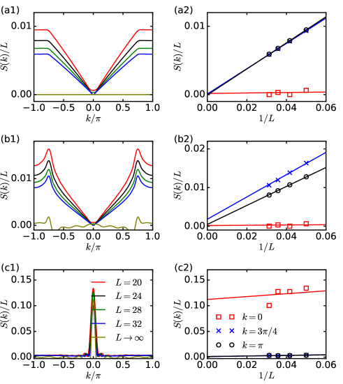
The left column of Fig. 1 plot for different with and , and the results for different system sizes are labeled by lines of different colors. The values of are obtained by the standard finite size scaling. The corresponding scaling details for three representative wave vectors, , , are shown in the right column of Fig. 1. We first pay attention to the two limits, and . As shown in Fig. 1(a1), for , the scaled structure factor generally decreases with the system size and eventually vanishes for all the wave vectors, which is the character of PM. The opposite limit with is demonstrated in Fig 1(c1). In this case, the peak at overwhelms values at other wave vectors, indicating the formation of FM. Something interesting happens if the coupling strength is tuned to an intermediate value . As shown in Fig. 1(b1), a sharp peak of appears at , which does not vanish even in the thermodynamic limit . This is a clear signal of a SDW phase with the ordering wave vector . With these results, we can expect that by varying the coupling strength from small to large, the system may undergo a transition from PM to SDW, and then end up with FM.
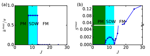
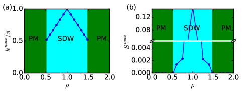
This process can be verified by monitoring the ordering wave vector and strength as functions of . Because of the inherent inversion symmetry of about , we hereafter restrict our discussion on the part. As depicted in Fig. 2, for relatively small coupling strength , is extrapolated to zero and the corresponding is not well defined, signaling the existence of PM. A SDW phase occurs for , in which both and take nonzero values. Tuning the coupling strength above , drops to zero, which is accompanied by monotonically increased , implying the formation of FM. It should be noticed that, within the SDW phase, keeps at a constant value irrespective of . In fact, in this phase is uniquely set by the bosonic density. Figure 3 demonstrates and in terms of for fixed and , where we find that the relation
| (15) |
is perfectly satisfied provided that the SDW phase is reached. Note that in Eq. (15), the integer number () is introduced to place the value of into the first Brillion zone .
These results encourages us to relate the bosonic SDW state with the Peierls state which usually emerges in the 1D fermionic system with lattice degrees of freedom Peierls1 . According to the Peierls theory in 1D, the ordering wave vector in a Peierls state is connected to the Fermi wave vector via , due to the perfectly nested Fermi surfaces Superradiance ; Fradkin13 . Remarkably, this relation also holds true in the SDW phase of our bosonic model, despite the absence of a Fermi surface. This suggests that a more comprehensive theoretical framework, capable of unifying the fermionic and bosonic cases, may be necessary to fully understand Peierls transitions.
The bosonic Peierls transition is not a perturbation effect, as can be inferred in Sec. III. Instead, it is essentially a strongly correlated effect which depends on the competition between relatively large and . This is in contrast with the 1D fermionic system, where the direct interactions between fermions is irrelevant to the formation of a Peierls state Fradkin13 . The effect of the bosonic Hubbard interaction is illustrated in Fig. 4, where we plot the variation of and in terms of for . As can be seen, the SDW phase can be formed only when the interaction is larger than some critical value . It is observed again that the ordering wave vector of the SDW remains at irrespective of , a principal feature of the Peierls state.
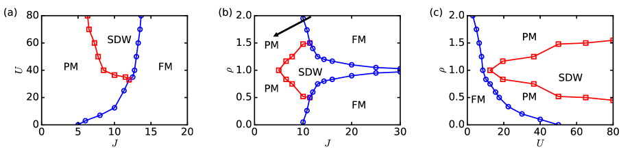
The competition of and for fixed density is quantitatively reflected in the phase diagram in Fig. 5(a). We can clearly find a lower bound of , below which the system evolves directly from PM to FM as increases. The transition from PM to FM becomes easier for smaller , consistent with the perturbation theory we developed in Subsection III.1. Above the lower bound of , the bosonic Peierls phase, which is more favored as increases, appears in between the PM and FM.
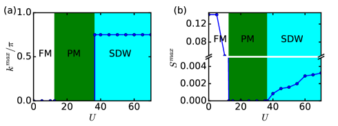
Given that the nature of the SDW phase is intimately connected to the bosonic density, it is then instructive to investigate the effect of density on various magnetic transitions. We map out the phase diagram in the plane with in Fig. 5(b). At any fixed , a general feature of the ground state is that it tend to be PM and FM for two opposite limit and , respectively. The SDW order is stabilized at an intermediate value of instead, and it is more favored when the system is closed to unit filling . The formation of FM at low bosonic densities can be understood by noting that the conduction bosons are sparsely distributed on the lattice, in which case the interaction is irrelevant. Because of a large antiferromagnetic Kondo coupling, different spin configurations of the localized moments behave like energy barriers hindering the motion of the conduction bosons. The most energetically favorable choice is to ferromagnetically align the localized spins, such that the bosons can freely move along the lattice, which lowers the energy by .
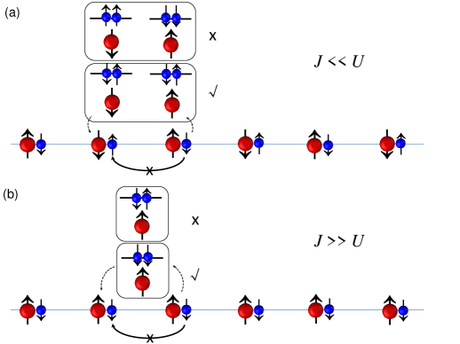
Nevertheless, the competition between and becomes crucial if the system is tuned to be around unit filling. In this case, each neighbor sites of the conduction bosons is likely to be occupied by another one. The direct tunneling of the conduction bosons between different sites is prohibited due to a large energy penalty costed by and . However, the energy can still be lowered, through exchanging excitations with some virtual states, by (), once the conduction bosons form an antiferromagnetic (ferromagnetic) spin configuration. From the viewpoint of superexchange mechanism, a relatively large () is amount to imposing a constraint on the intermediate virtual states such that double occupancy of the conduction bosons with parallel (antiparallel) sspin is excluded from the Hilbert space (see Fig. 6 for illustration). It thus follows that the SDW phase (FM) is energetically more favorable for at least (). This feature becomes clearer in the phase diagram, as we show in Fig. 5(c). It is seen that, while the FM is generally stabilized at small , the SDW phase can be formed only when and the bosonic density is not far away from . As increases, the range of , where the SDW order can exist, grows up. Notice that at unit filling, the critical point of , above which the FM is destabilized, is estimated as , in agreement with the perturbation results we derived in Subsection III.2.
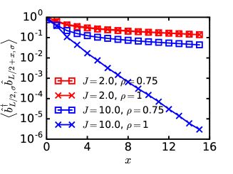
Another important feature accompanied with the SDW order is the absense of the off-diagonal bosonic long-range orders at commensurate fillings. The superfluid correlation function for different densities and Kondo couplings are depicted in Fig. 7. It is shown that the correlation with and different presents long-range order, which, as expected, inherits the superfluid nature of the Bose-Hubbard model. For larger Kondo couplings at which the SDW order is stabilized, on the other hand, the property of the superfluid correlation depends strongly on the commensurability of . As plotted by blue curves in Fig. 7, while the long-range feature of the superfluid correlation remains at incommensurate fillings (i.e., takes non-integer values), at unit filling decreases exponentially with the distance , indicating the absence of the off-diagonal bosonic long-range orders.
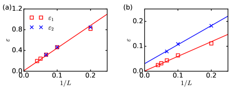
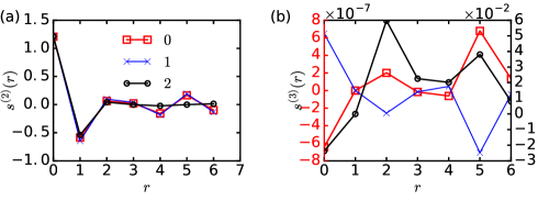
It is known that a Peierls gap naturally emerges in the fermionic density wave phase Peierls1 ; Holstein . This feature is also present in the bosonic Peierls state here. To see this clearly, one can analyze the scaling of the lowest excitation energies with the system size, where is the energy of the th lowest eigenstate of the Hamiltonian (1). In the PM phase with superfluid character, we have found that the decrease rapidly with the system size and vanishes in the thermodynamic limit, as seen in Fig. 8(a). This implies that the ground state here is unique and gapless, as expected for a standard superfluid. However, the scaling of in the SDW phase exhibits completely different behavior. As shown in Fig. 8(b), while is extrapolated to zero as , the energy differences between the two lowest eigenstates and the higher excited states remain finite in the thermodynamic limit. This means that the ground state of the SDW is twofold degenerate in the limit. This degeneracy originates from the symmetry of the system with respect to the spin flip transformations and . To demonstrate this, we have calculated the two- and three-body spin correlations, and , respectively, under the three lowest eigenstates in the SDW phase. As can be seen in Figs. 9(a) and 9(b), while calculated for the first exited state tends to be the same value as for the ground state, the quantity under the second exited state shows dramatically different configuration. Further more, the three-body correlation for the two lowest eigenstates presents exactly inverted patterns, which is also quite different from that for the higher eigenstates. Therefore, both the two lowest eigentates are bosonic Peierls states with finite excitation gaps in the thermodynamic limit. It is thus interesting to find that, although possessing both diagonal and off-diagonal long-range correlations, the bosonic Peierls phase at incommensurate fillings is different from the standard supersolid because of its gapped nature Hubbard .
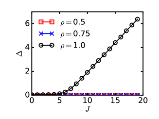
The appearance of diagonal density wave orders in the ground state is often accompanied with a nonzero charge gap, i.e., the state is incompressible with zero compressibility . Figure 10 plots the charge gap , which has been extrapolated to the limit, in terms of for and different . It is observed that at commensurate bosonic fillings, a finite charge gap indeed exists in the SDW phase, consistent with the results from perturbation theory (see Subsection III.2). However, the SDW phase with incommensurate bosonic fillings turns out to be compressible with vanishingly small charge gap. Therefore, although the ground state keeps gapped throughout the SDW phase, its compressibility depends crucially on the bosonic density. The concurrence of a excitation gap, a diagonal long-range order, and a nonzero compressibility can be understood under the single-particle fermionic picture. When adding or removing particles from the fermi-lattice system, the band structure, especially the position of the gap, is modified at the same time according to the relation . This lattice relaxation effect can prevent the gap penalty when changing the particle density, giving rise to a nonzero compressibility. While the relation still holds in the bosonic Peierls state, the underlying mechanism can not be understood on a single-particle level, as the Fermi surface picture is lacking BP1 . Its microscopic origin for general particle densities should be traced back to the strong boson-boson and boson-lattice correlation, the exploration of which is beyond the scope of this paper and we leave to future work.
V Possible experimental implementation
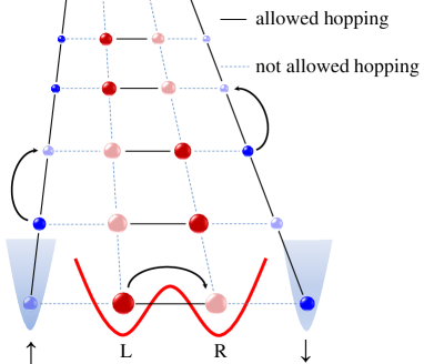
The most convenient way to realize the bosonic IKL is to properly control ultracold bosonic atoms in optical lattices. The conduction bosons and localized magnetic moments can be realized by loading atoms in energy bands with different mobilities BHighOL1 ; BHighOL2 ; BHighOL3 , or populating optical lattices by alkaline-earth-metal atoms which may experience different trapping potentials, depending on their orbital angular momenta HighOL3 ; HighOL4 ; HighOL5 ; HighOL6 ; HighOL7 ; HighOL8 . The Ising anisotropy of the Kondo coupling can be easily achieved by various methods, including the confinement-induced resonances Anisotropy1 and the laser-induced inter-channel coupling Anisotropy2 ; Anisotropy3 . We here provide an alternative way to experimentally implement our model. The basic idea is to simulate the spin degrees of freedom by lattice sites in real space. As shown in Fig. 11, we consider first a gas of ultracold bosonic atoms confined in two independent 1D chains, which are arranged to be parallel to each other and can therefore represent different spin index of the conduction bosons. Each chain of the bosonic atoms is described by the Bose-Hubbard Hamiltonian. Such a scenario can be engineered by imposing an optical superlattice SuperOL1 ; SuperOL2 . Two additional chains of ultracold atoms, tightly trapped either by optical tweezers or a second optical superlattice with a double-well structure, are introduced in between the original two potential minima of the conduction bosons. These tightly trapped atoms, which we refer to as localized atoms, form a ladder structure in real space. While the particle hopping along the two legs of the ladder is forbidden by large energy barriers, a weak tunneling is allowed along the rung. We further assume that each double well is occupied by only one localized atom, which can be realized adiabatically in experiment. The Hamiltonian describing the particle dynamics in such a configuration can be readily written as
| (16) | |||||
where with () the creation (annihilation) operator of the localized atoms. The subscript () labels the position of the localized atoms in each double well. The first two terms of the Hamiltonian (16) are the Bose-Hubbard Hamiltonians for the conduction bosons, and the third term describes the nearest neighbor interactions between the conduction bosons and the localized atoms. The tunnelings of the localized atoms in each double well are accounted for by the last term of the Hamiltonian (16). Making use of the schwinger transformations , , , and the constraint , the Hamiltonian (16) immediately reduces to the bosonic IKL Hamiltonian (1) with the substitution of the coupling constants and . In this sense, the localized atoms play the role of localized magnetic moments in the bosonic IKL, and the spin degrees of freedom are encoded in the two minima of each double well. Hamiltonian (16) has the advantage that all parameters can be tuned independently. For example, and can be controlled by the depths of the optical traps, and and can be tuned through the Feshbach resonance Feshbach or the confinement induced resonance Anisotropy1 .
VI Conclusion
In conclusion, we have studied a bosonic version of the 1D IKL, in which the electrons are replaced by spin- bosons. Utilizing a perturbative analysis and the numerical DMRG method, we have characterized the phases of the system in different parameters regimes. Apart from the PM and FM, a Peierls-like state, characterized by a long-range SDW order and a nonzero excitation gap, has been revealed. We have also discussed the possibility of implementing the model using ultracold atoms in optical lattices.
Acknowledgments
This work is supported by the National Key R&D Program of China under Grant No. 2022YFA1404201, the National Natural Science Foundation of China (NSFC) under Grant No. 12174233, 12034012 and 12004230, the Research Project Supported by Shanxi Scholarship Council of China and Shanxi ’1331KSC’. Our simulations make use of the ALPSCore library ALPS , based on the original ALPS project ALPS2 .
Appendix A Derivation of the effective spin Hamiltonian in the strong coupling limit
We here derive the effective Hamiltonian (1) in the main text based on the second order perturbation theory. Given that the effective Hamiltonian involves only on-site and nearest-neighbor interactions, our derivation will start from a two-site system, the extension of which to a lattice is straightforward. Since we consider the strong coupling limit with and , it is convenient to write the original two-site Hamiltonian as the addition of two parts,
where
and
Here, is the zeroth order Hamiltonian which can be treated exactly and denotes the perturbation part. The state basis spanning the whole Hilbert space can be chosen as the product states . We further assume the commensurate filling on each site, and then the ground-state manifold is constituted by states , where the magnetization is fixed by Eq. (6). Note that by this notation, the antiferromagnetic nature of the Kondo coupling has been taken into consideration. The state is fourfold degenerate with respect to the free choice of and . This degeneracy can be lifted by virtual transitions to some exited states . These virtual exited states can either be charge-like or spin-like, depending on the ways they are connected to the ground states. The charge-like (spin-like) exited states can be straightforwardly obtained by acting the hopping (transverse field) term of on the states . Using this principle, we can write the charge-like exited states and their corresponding energies as
| (17) |
| (18) |
| (19) |
Similarly, the spin-like exited states and energies are obtained as
| (20) |
With the exited states (17)-(20) and the low energy states , the effective Hamiltonian can be represented in terms of the matrix elements of the perturbation via the formula Counterflow
| (21) |
where labels the exited states , and and represent the exited- and ground-state eigenenergies of , respectively. Inserting Eqs. (17)-(20) into Eq. (21), we can write the effective Hamiltonian in terms of the spin operators and , i.e.,
| (22) | |||||
where the coupling constants and are defined in Eqs. (III.2)-(III.2). Extending the two-site Hamiltonian (22) to a lattice, we immediately obtain the effective Hamiltonian (9) in the main text.
References
- (1) A. Altland and B. Simons, Condensed Matter Field Theory (Cambridge University Press, Cambridge, England, 2006).
- (2) E. B. Herbold and V. F. Nesterenko, Shock wave structure in a strongly nonlinear lattice with viscous dissipation, Phys. Rev. E 75, 021304 (2007).
- (3) P. Harvey, C. Durniak, D. Samsonov, and G. Morfill, Soliton interaction in a complex plasma, Phys. Rev. E 81, 057401 (2010).
- (4) D. Frydel and Y. Levin, Soft-particle lattice gas in one dimension: One- and two-component cases, Phys. Rev. E 98, 062123 (2018).
- (5) Y. Guo, R. M. Kroeze, B. P. Marsh, S. Gopalakrishnan, J. Keeling, and B. L. Lev, An optical lattice with sound, Nature 599, 211 (2021).
- (6) R. Peierls, Quantum Theory of Solids, International Series of Monographs on Physics (Clarendon Press, Oxford, 1955).
- (7) D. González-Cuadra, P. R. Grzybowski, A. Dauphin, and M. Lewenstein, Strongly Correlated Bosons on a Dynamical Lattice, Phys. Rev. Lett. 121, 090402 (2018).
- (8) D. González-Cuadra, A. Bermudez, P. R. Grzybowski, M. Lewenstein, and A. Dauphin, Intertwined topological phases induced by emergent symmetry protection, Nature Communications 10, 2694 (2019).
- (9) D. González-Cuadra, A. Dauphin, P. R. Grzybowski, and M. Lewenstein, A. Bermudez, Dynamical Solitons and Boson Fractionalization in Cold-Atom Topological Insulators, Phys. Rev. Lett. 125, 265301 (2020).
- (10) C. Rylands, Y. Guo, B. L. Lev, J. Keeling, and V. Galitski, Photon-Mediated Peierls Transition of a 1D Gas in a Multimode Optical Cavity, Phys. Rev. Lett. 125, 010404 (2020).
- (11) A. C. Hewson, The Kondo Problem to Heavy Fermions (Cambridge University Press, Cambridge, England 1993).
- (12) P. Coleman and A. H. Nevidomskyy, Frustration and the Kondo effect in heavy fermion materials, Journal of Low Temperature Physics 161, 182 (2010).
- (13) F. Steglich and S. Wirth, Foundations of heavy-fermion superconductivity: lattice Kondo effect and Mott physics, Rep. Prog. Phys. 79, 084502 (2016).
- (14) C. L. Seaman, M. B. Maple, B. W. Lee, S. Ghamaty, M. S. Torikachvili, J.-S. Kang, L. Z. Liu, J. W. Allen, and D. L. Cox, Evidence for non-Fermi liquid behavior in the Kondo alloy Y1-xUxPd3, Phys. Rev. Lett. 67, 2882 (1991).
- (15) E. Miranda, V. Dobrosavljević, and G. Kotliar, Disorder-Driven Non-Fermi-Liquid Behavior in Kondo Alloys, Phys. Rev. Lett. 78, 290 (1997).
- (16) A. Principi, G. Vignale, and E. Rossi, Kondo effect and non-Fermi-liquid behavior in Dirac and Weyl semimetals, Phys. Rev. B 92, 041107(R) (2015).
- (17) A. F. Otte, M. Ternes, K. von Bergmann, S. Loth, H. Brune, C. P. Lutz, C. F. Hirjibehedin, and A. J. Heinrich, The role of magnetic anisotropy in the Kondo effect, Nat. Phys. 4, 847 (2008).
- (18) M. Misiorny, I. Weymann, and J. Barnaś, Influence of magnetic anisotropy on the Kondo effect and spin-polarized transport through magnetic molecules, adatoms, and quantum dots, Phys. Rev. B 84, 035445 (2011).
- (19) M. Misiorny, M. Hell, and M. R. Wegewijs, Spintronic magnetic anisotropy, Nat. Phys. 9, 801 (2013).
- (20) A. E. Sikkema, W. J. L. Buyers, I. Affleck, and J. Gan, Ising-Kondo lattice with transverse field: A possible f-moment Hamiltonian for URu2Si2, Phys. Rev. B 54, 9322 (1996).
- (21) H. Ishizuka and Y. Motome, Partial Disorder in an Ising-Spin Kondo Lattice Model on a Triangular Lattice, Phys. Rev. Lett. 108, 257205 (2012).
- (22) H. Ishizuka and Y. Motome, Thermally induced phases in an Ising Kondo lattice model on a triangular lattice: Partial disorder and Kosterlitz-Thouless state, Phys. Rev. B 87, 155156 (2013).
- (23) H. Ishizuka and Y. Motome, Loop liquid in an Ising-spin Kondo lattice model on a kagome lattice, Phys. Rev. B 88, 081105(R) (2013).
- (24) H. Ishizuka and Y. Motome, Exotic magnetic phases in an Ising-spin Kondo lattice model on a kagome lattice, Phys. Rev. B 91, 085110 (2015).
- (25) J. Shin, Z. Schlesinger, and B. S. Shastry, Kondo-Ising and tight-binding models for TmB4, Phys. Rev. B 95, 205140 (2017).
- (26) S. Tsuda, C. L. Yang, Y. Shimura, K. Umeo, H. Fukuoka, Y. Yamane, T. Onimaru, T. Takabatake, N. Kikugawa, T. Terashima, H. T. Hirose, S. Uji, S. Kittaka, and T. Sakakibara, Metamagnetic crossover in the quasikagome Ising Kondo-lattice compound CeIrSn, Phys. Rev. B 98, 155147 (2018).
- (27) B. Li, J.-Q. Yan, D. M. Pajerowski, E. Gordon, A.-M. Nedić, Y. Sizyuk, L. Ke, P. P. Orth, D. Vaknin, and R. J. McQueeney, Competing Magnetic Interactions in the Antiferromagnetic Topological Insulator MnBi2Te4, Phys. Rev. Lett. 124, 167204 (2020).
- (28) W.-W. Yang, J. Zhao, H.-G. Luo, and Y. Zhong, Exactly solvable Kondo lattice model in the anisotropic limit, Phys. Rev. B 100, 045148 (2019).
- (29) W.-W. Yang, Y. Zhong, and H.-G. Luo, Hexagonal Ising-Kondo lattice: An implication for intrinsic antiferromagnetic topological insulator, Phys. Rev. B 102, 195141 (2020).
- (30) W.-W. Yang, Y.-X. Li, Y. Zhong, and H.-G. Luo, Doping a Mott insulator in an Ising-Kondo lattice: Strange metal and Mott criticality, Phys. Rev. B 104, 165146 (2021).
- (31) X. Zhou, J. Fan, and S. Jia, Magnetic order and strongly correlated effects in the one-dimensional Ising-Kondo lattice, Phys. Rev. B 109, 195112 (2024).
- (32) F. Schäfer, T. Fukuhara, S. Sugawa, Y. Takasu, and Y. Takahashi, Tools for quantum simulation with ultracold atoms in optical lattices, Nat. Rev. Phys. 2, 411 (2020).
- (33) B. Yang, H. Sun, C.-J. Huang, H.-Y. Wang, Y. Deng, H.-N. Dai, Z.-S. Yuan, and J.-W. Pan, Cooling and entangling ultracold atoms in optical lattices, Science 369, 550 (2020).
- (34) Y. Guo, R. M. Kroeze, B. P. Marsh, S. Gopalakrishnan, J. Keeling, and B. L. Lev, An optical lattice with sound, Nature 599, 211 (2021).
- (35) J.-y. Choi, Quantum simulations with ultracold atoms in optical lattices: past, present and future, Journal of the Korean Physical Society 82, 875 (2023).
- (36) D. Malz and J. I. Cirac, Few-Body Analog Quantum Simulation with Rydberg-Dressed Atoms in Optical Lattices, PRX Quantum 4, 020301 (2023).
- (37) T. Müller, S. Fölling, A. Widera, and I. Bloch, State Preparation and Dynamics of Ultracold Atoms in Higher Lattice Orbitals, Phys. Rev. Lett. 99, 200405 (2007).
- (38) G. Wirth, M. Ölschläger, and A. Hemmerich, Evidence for orbital superfluidity in the P-band of a bipartite optical square lattice, Nat. Phys. 7, 147 (2011).
- (39) Y. Zhong, Y. Liu, and H.-G. Luo, Simulating heavy fermion physics in optical lattice: Periodic Anderson model with harmonic trapping potential, Frontiers of Physics 12, 127502 (2017).
- (40) L. Riegger, N. Darkwah Oppong, M. Höfer, D. R. Fernandes, I. Bloch, and S. Fölling, Localized Magnetic Moments with Tunable Spin Exchange in a Gas of Ultracold Fermions, Phys. Rev. Lett. 120, 143601 (2018).
- (41) M. Kanász-Nagy, Y. Ashida, T. Shi, C. P. Moca, T. N. Ikeda, S. Fölling, J. I. Cirac, Gergely Zaránd, and E. A. Demler, Exploring the anisotropic Kondo model in and out of equilibrium with alkaline-earth atoms, Phys. Rev. B 97, 155156 (2018).
- (42) X. Zhou, S. Jin, and J. Schmiedmayer, Shortcut loading a Bose–Einstein condensate into an optical lattice, New J. Phys. 20 055005 (2018).
- (43) R. Zhang, Y. Cheng, P. Zhang, and H. Zhai, Controlling the interaction of ultracold alkaline-earth atoms, Nat. Rev. Phys. 2, 213 (2020).
- (44) K. Ono, Y. Amano, T. Higomoto, Y. Saito, and Y. Takahashi, Observation of spin-exchange dynamics between itinerant and localized 171Yb atoms, Phys. Rev. A 103, L041303 (2021).
- (45) L.-M. Duan, Controlling ultracold atoms in multi-band optical lattices for simulation of Kondo physics, Europhys. Lett. 67, 721 (2004).
- (46) M. Foss-Feig and A. M. Rey, Phase diagram of the bosonic Kondo-Hubbard model, Phys. Rev. A 84, 053619 (2011).
- (47) T. Flottat, F. Hébert, V. G. Rousseau, R. T. Scalettar, and G. G. Batrouni, Bosonic Kondo-Hubbard model, Phys. Rev. B 92, 035101 (2015).
- (48) S. R. White, Density matrix formulation for quantum renormalization groups, Phys. Rev. Lett. 69, 2863 (1992).
- (49) U. Schollwök, The density-matrix renormalization group, Rev. Mod. Phys. 77, 259 (2005).
- (50) A. Gagge and J. Larson, Superradiance, bosonic Peierls distortion, and lattice gauge theory in a generalized Rabi-Hubbard chain, Phys. Rev. A 102, 063711 (2020).
- (51) A. Auerbach, Interacting Electrons and Quantum Magnetism (Springer-Verlag, New York, 1994).
- (52) Y. Chen, Z. Yu, and H. Zhai, Superradiance of Degenerate Fermi Gases in a Cavity, Phys. Rev. Lett. 112, 143004 (2014).
- (53) E. Fradkin, Field Theories of Condensed Matter Physics (Cambridge University Press, Cambridge, 2013).
- (54) E. Jeckelmann, C. Zhang, and S. R. White, Metal-insulator transition in the one-dimensional Holstein model at half filling, Phys. Rev. B 60, 7950 (1999).
- (55) T. Chanda, L. Barbiero, M. Lewenstein, M. J. Mark, and J. Zakrzewski, Recent progress on quantum simulations of non-standard Bose-Hubbard models, arXiv:2405.07775 (2024).
- (56) R. Zhang, D. Zhang, Y. Cheng, W. Chen, P. Zhang, and H. Zhai, Kondo effect in alkaline-earth-metal atomic gases with confinement-induced resonances, Phys. Rev. A 93, 043601 (2016).
- (57) M. Nakagawa and N. Kawakami, Laser-Induced Kondo Effect in Ultracold Alkaline-Earth Fermions, Phys. Rev. Lett. 115, 165303 (2015).
- (58) T.-S. Deng, W. Zhang, and W. Yi, Tuning Feshbach resonances in cold atomic gases with interchannel coupling, Phys. Rev. A 96, 050701(R) (2017).
- (59) J. Sebby-Strabley, M. Anderlini, P. S. Jessen, and J. V. Porto, Lattice of double wells for manipulating pairs of cold atoms, Phys. Rev. A 73, 033605 (2006).
- (60) M. Atala, M. Aidelsburger,Mi. Lohse, J. T. Barreiro, B. Paredes and I. Bloch, Observation of chiral currents with ultracold atoms in bosonic ladders, Nat. Phys. 10, 588 (2014).
- (61) T. Köhler, K. Góral, and P. S. Julienne, Production of cold molecules via magnetically tunable Feshbach resonances, Rev. Mod. Phys. 78, 1311 (2006).
- (62) A. Gaenko, A. Antipov, G. Carcassi, T. Chen, X. Chen, Q. Dong, L. Gamper, J. Gukelberger, R. Igarashi, S. Iskakov, M. Konz, J. LeBlanc, R. Levy, P. Ma, J. Paki, H. Shinaoka, S. Tödo, M. Troyer, and E. Gull, Updated core libraries of the ALPS project, Comp. Phys. Comm. 213, 235 (2017).
- (63) B. Bauer, L. D. Carr, H. G. Evertz, A. Feiguin, J. Freire, S. Fuchs, L. Gamper, J. Gukelberger, E. Gull, S. Guertler, A. Hehn, R. Igarashi et al., The ALPS project release 2.0: open source software for strongly correlated systems, Journ. of Stat. Mech.: Theor. and Exp. 2011, P05001 (2011).
- (64) A. B. Kuklov and B. V. Svistunov, Counterflow Superfluidity of Two-SpeciesUltracold Atoms in a Commensurate Optical Lattice, Phys. Rev. Lett. 90, 100401 (2003).