Graph Neural Networks-based Parameter Design towards Large-Scale Superconducting Quantum Circuits for Crosstalk Mitigation

Abstract

To demonstrate supremacy of quantum computing, increasingly large-scale superconducting quantum computing chips are being designed and fabricated, sparking the demand for electronic design automation in pursuit of better efficiency and effectiveness. However, the complexity of simulating quantum systems poses a significant challenge to computer-aided design of quantum chips. Harnessing the scalability of graph neural networks (GNNs), we here propose a parameter designing algorithm for large-scale superconducting quantum circuits. The algorithm depends on the so-called ’three-stair scaling’ mechanism, which comprises two neural-network models: an evaluator supervisedly trained on small-scale circuits for applying to medium-scale circuits, and a designer unsupervisedly trained on medium-scale circuits for applying to large-scale ones. We demonstrate our algorithm in mitigating quantum crosstalk errors, which are commonly present and closely related to the graph structures and parameter assignments of superconducting quantum circuits. Parameters for both single- and two-qubit gates are considered simultaneously. Numerical results indicate that the well-trained designer achieves notable advantages not only in efficiency but also in effectiveness, especially for large-scale circuits. For example, in superconducting quantum circuits consisting of around $870$ qubits, the trained designer requires only $27$ seconds to complete the frequency designing task which necessitates $90$ minutes for the traditional Snake algorithm. More importantly, the crosstalk errors using our algorithm are only $51\%$ of those produced by the Snake algorithm. For specific superconducting quantum chips in real experiments, the designer’s outputs can serve as initial iteration values of traditional optimizers to enhance the designing performances. Overall, this study initially demonstrates the advantages of applying graph neural networks to design parameters in quantum processors, and provides insights for systems where large-scale numerical simulations are challenging in electronic design automation.

I Introduction

Quantum computing may have applications in fields including cryptography [1], databases [2], computational chemistry [3], and machine learning [4]. Thus, large-scale quantum information processors are demanded to fully manifest the quantum advantages. Among various quantum computing platforms including neutral atom arrays [5] and trapped irons [6], superconducting quantum computing system based on Josephson junctions is a leading candidate [7, 8, 9, 10]. Qubit numbers and the scales of quantum processors implemented by superconducting quantum electronic circuits (SQECs) are rapidly increasing. The numbers of quantum elements in superconducting quantum computing chip are now more than hundreds and even reach thousands, e.g. in chips of IBM company [11]. Due to the rapid growth of circuit complexity, the analysis and manual design on these large-scale SQECs are becoming challenging. Thus, the design automation for quantum computing systems aided by electronic computers or artificial intelligence is attracting more and more attentions [12, 13, 14, 15, 16, 17, 18, 19].

For semiconductor integrated circuits, electronic design automation (EDA), also known as electronic computer-aided design, has achieved a high level of maturity [20]. Additionally, artificial intelligence has recently been applied to enhance the efficiency of semiconductor integrated circuit design automation [21, 22, 23]. However, due to the substantial differences in fundamental components, operating conditions, and operational modes between semiconductor integrated circuits and SQECs, it is difficult to directly apply traditional EDA techniques to the design of SQECs. Moreover, as the dimension of the Hilbert space exponentially scales with the number of qubits in quantum processors [24], the evaluation of the designed SQECs through numerical simulations is becoming a challenging task, which further complicates the automated design towards large-scale quantum processors. In this study, we focus on the automated design of working parameters in SQECs with given structures. In previous studies, the Snake algorithm was developed for designing parameters in large-scale SQECs [25, 26] and was applied in the context of Google’s Sycamore processor [7].

Similar to the graphic representation of semiconductor integrated circuits, SQECs can be readily conceptualized as graph structures. This inspires us to achieve automated parameter design for large-scale SQECs by utilizing the scalability of graph neural networks [27, 28] (GNNs). Within the graphic structures, the qubits for storing and processing quantum information are considered as nodes. Meanwhile, nearest neighbor coupled-qubit pairs represent edges in the graphs. The configuration of parameters on each node and edge can significantly impact the performance of quantum computing. Especially some of the parameters may have graph-dependent effects and need to be configured differently on different nodes and edges. Thus, GNNs are well-suited for designing these parameters. From mathematical point of view, the parameter designing task of SQECs can be interpreted as an extension of graph coloring problem [29, 30] (GCP), which involves node and edge colors, continuous coloring, and considerations for the impact of higher-order neighbors.

In this work, a GNNs-based algorithm for designing parameters in SQECs is proposed. The realization of the algorithm requires two neural-network models, an evaluator for estimating the quality of parameter assignments and a designer for designing an optimal parameter assignment based on the evaluator’s feedback. The influence of considered parameters is assumed to be localized. Therefore, the evaluator, comprising some graph-based multi-layer perceptrons [31, 32] (MLPs), is supervisedly trained on several small-scale SQECs to avoid direct simulations on larger quantum processors. Utilizing the errors and corresponding gradients computed by the evaluator, the GNNs-based designer is unsupervisedly trained on randomly generated medium-scale graphs. Leveraging the scalability of GNNs, the trained designer is directly applied to different graphs in terms of structure or scale. In such way, the parameter designing algorithm can be facilitated for large-scale SQECs.

We further demonstrate the proposed algorithm with the task of designing frequency assignments on SQECs such that quantum crosstalk errors can be mitigated. Quantum crosstalk is commonly present in superconducting quantum computing systems [33, 34, 35, 36, 37, 38, 39, 40]. It refers to the undesired interference experienced by other qubits when a quantum operation is applied to specific qubits. Quantum crosstalk comes from some fundamental theories in quantum physics, including perturbation theory [41], dressing states [42], and conservation laws (See supplementary materials [43]), thus crosstalk errors are challenging to be completely eliminated. Qualitatively, with other parameters given, the quantum crosstalk error between two qubits is inversely related to their frequency difference and their distance within the graph [33, 35]. Both single- and two-qubit operations are involved in our study, which can be combined to implement universal quantum computation [44]. The quantum operations relate to node and edge frequencies simultaneously, so both frequencies are taken into account in our study. When numerically simulating quantum crosstalk errors, we consider various factors that may influence the errors, such as residual couplings between high-order neighboring qubits [33, 45], the couplers connected between qubits [46], and higher excitations of these quantum modes [47].

The implementation of the proposed algorithm mainly includes the following steps. First, the crosstalk errors of around $100,000$ random frequency assignments on three $6$-qubit graphs are numerically simulated to train, validate and test the evaluator. To further verify the evaluator’s generalization ability, additional validation and testing are also performed on two other $6$-qubit graphs. Thanks to the extra validation and testing, along with the localized property of quantum crosstalk errors, the evaluator trained on $6$-qubit graphs can be applied to larger graphs. Based on the errors and corresponding gradients obtained from the trained evaluator, we further unsupervisedly train the designer on the randomly generated medium-scale graphs containing approximately $54$, $103$ and $218$ nodes, and then apply it to various large-scale graphs. The well-trained designer demonstrates significant advantages over traditional methods in terms of both efficiency and effectiveness for all tested graph scales, ranging from $31$ to $870$ nodes. For instance, in large-scale SQECs comprising $870$ qubits, the trained designer achieves an average crosstalk error of $0.0090$ within $27$ seconds, whereas the Snake algorithm takes $90$ minutes to reach an average crosstalk error of $0.0178$.

To our best knowledge, we here first apply graph neural networks to design parameters in large-scale quantum information processors, e.g., SQECs. Especially when concerning the scales, the evaluator trained on small-scale graphs is applied to estimate errors on larger graphs, while the designer trained on medium-scale graphs can be utilized to design parameters for large-scale ones. This ’three-stair scaling’ technique provides insights for the systems where numerical simulations are challenging in EDA. Furthermore, not only the designer demonstrates superior performance and scalability in numerical results, but the designed parameters can also serve as initial optimization values for closely approximating the optimal settings in real experiments. This feature facilitates the adaptation to specific quantum processors, streamlining the experimental process.

II Algorithm

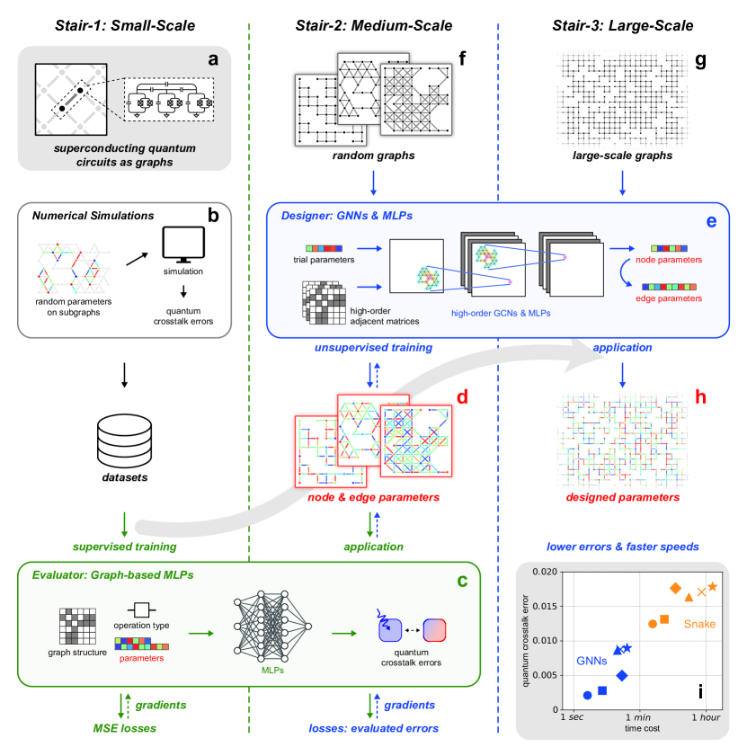
Figure 1: Algorithm. In the ’three-stair scaling’ technique, two neural-network models, i.e., the evaluator and the designer, are trained and applied to connect the three scales. The graphic representation of SQECs is shown in a, where graph’s nodes and edges are represented as dots and segments. Throughout the article, nodes or edges are colored with gray when concerning the structure of graphs. While they are colored with rainbow colors when concerning their parameters, where different colors represent different parameters. In b, random parameters are sampled on several different small-scale subgraphs (e.g., the colored parts, each with $6$ qubits) in a larger-scale graph. Quantum crosstalk errors are numerically solved to construct datasets for the evaluator. The evaluator, illustrated in c, utilizes multiple graph-based MLPs to predict quantum crosstalk errors based on the graph structure, parameter assignment, and operation type. The MLPs are supervisedly trained according to the MSE losses and the corresponding gradients. The evaluator trained on small-scale graphs is applied to medium-scale graphs, e.g., d with around $54$ qubits in this study. Then using the evaluated errors and their gradients, the designer shown in e is unsupervisedly trained on random medium-scale graphs such as the graphs in f. The designer assigns parameters for f to obtain d, which integrates GNNs and MLPs to determine optimal node and edge parameters based on the input graphs and trial parameters. Finally, the trained designer can be directly applied to graphs of various structures and scales, including large-scale ones. The example of applying the designer on a large-scale graph is demonstrated with g and h, e.g., a SQEC with $870$ qubits. The comparison of our algorithm (GNNs, with blue markers) and traditional algorithm (Snake, with orange markers) is plotted in i. The horizontal axis represents the time cost, and the vertical axis represents the quantum crosstalk error. The tested graphs range from medium-scale to large-scale, and different scales are represented by different markers, e.g., square, triangle and star. More details about the tests can be found in Fig. 4, and the well-trained designer achieves notable advantages in both efficiency and effectiveness.

Our GNNs-based algorithm can design parameters for a coupled-qubit graph conceptualized from a given SQEC, in which various parameters of nodes (qubits) and edges (coupled-qubit pairs) need to be designed for mitigating errors of quantum computing [26, 33]. Some of the parameters are considered graph-independent, which can be designed and optimized individually. While other parameters may have graph-dependent effects, i.e., the parameters of certain node or edge may impact the neighboring nodes and edges. This requires a comprehensive consideration of the entire graph during the designing process. Furthermore, the error dependence on the graph-dependent parameters is complicated, for example, parameters optimized for one node may cause large errors on other nodes. Consequently, powerful algorithms should be implemented to achieve the optimal design of the parameters. Thus, the following studies are based on the graphs conceptualized from SQECs, as schematically shown in Fig. 1(a).

The GNNs-based parameter designing algorithm considers parameters of nodes and edges, and includes errors from influences of higher-order neighbors (e.g., 2-hop, 3-hop neighbors). As illustrated in Fig. 1, graphs with three scales are involved, i.e., small-scale graphs denoted as stair-$1$, medium-scale graphs denoted as stair-$2$, and large-scale graphs denoted as stair-$3$. The three stairs are connected via two neural-network models: the evaluator and the designer. The evaluator is supervisedly trained on small-scale graphs, and is applied to medium-scale graphs. While the designer is unsupervisedly trained on medium-scale graphs to be applied to large-scale graphs. First, as shown in Fig. 1(b), training data for the evaluator is collected on several small graphs, where a variety of parameter assignments are randomly generated as input labels, and corresponding errors are numerically simulated to serve as output labels. Then the evaluator is trained through supervised learning. As demonstrated in Fig. 1(c), the evaluator employs multiple graph-based MLPs to predict errors based on the graph structure, parameter assignment, and type of quantum operations. When training the evaluator, mean square errors (MSEs) are calculated as loss functions, and the corresponding gradients are used for backpropagation. After training the evaluator, it can be directly applied for parameter assignments on medium-scale graphs, e.g., Fig. 1(d). Unsupervised learning is employed to train the designer using the errors obtained by the evaluator. As illustrated in Fig. 1(e), the designer integrates GNNs and MLPs to determine optimal parameters for nodes and edges based on the input graphs and trial parameters. In each training iteration, a batch of medium-scale graphs is randomly created as input data for the designer, e.g., in Fig. 1(f), some of the nodes and edges are randomly removed from several fundamental graphs. Subsequently, the designer outputs a parameter assignment for each graph as shown with Fig. 1(d), and the corresponding average error is estimated using the trained evaluator. After training the designer on medium-scale random graphs, the scalability of GNNs enables the trained designer to be directly applied to graphs of various structures and scales, including large-scale ones as exemplified with Figs. 1(g) and (h). Additionally, leveraging the parallelism capabilities of machine learning frameworks such as PyTorch [48] and TensorFlow [49], we can further enhance the performance on specific graphs by generating diverse sets of trial parameter assignments and utilizing the designer in batches.

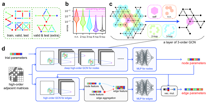
Figure 2: Details for the proposed algorithm. a. The small-scale graphs for training, validating, and testing the evaluator, which are the most common qubit-coupling structures. The node and edge parameters are randomly sampled to generated the datasets. Each graph contains $6$ nodes, the left $3$ graphs are used for training, validating, and testing. While the right $2$ graphs are used for extra validating and testing, guaranteeing the evaluator’s generalization ability to different underlying structures. b. The exponentially decay of the interplay between two nodes with their distance. Dataset for plotting b is obtained by simulating single-qubit $R_{X}$ operations on a small-scale graph. The horizontal axis represents the distance between nodes, and the vertical axis represents the error in logarithmic coordinates. The width of the plot at different values indicates the amount of the data. Since only the errors ranging from $10^{-4}$ to $10^{-1}$ are concerned, the crosstalk errors between nodes with far distances can be neglected. This guarantees the evaluator’s generalization ability to larger-scale graphs. c. A layer of 3-order GCN. The node features of itself (magenta), its nearest neighbor nodes (orange), its $2$-hop nodes (green), and its $3$-hop nodes (blue) are aggregated. d. The detailed architecture of the designer. High-order adjacent matrixes and trial node parameters are input to the designer. First, a deep high-order GCN and an MLP can assign parameters for each node, which constitute part of the designer’s output. Second, these node parameters serve as inputs for another high-order GCN to output new node features, which are then aggregated by edges and fed into another MLP. The MLP outputs each edge parameter’s selection preferences $p_{i},p_{j}$ from its two nodes’ parameters $\omega_{i},\omega_{j}$. Then vector multiplication (vec. mul.) is performed to obtain the corresponding edge parameter, $\omega_{ij}=p_{i}\omega_{i}+p_{j}\omega_{j}$. Thus the edge parameters are assigned to constitute another part of the designer’s output. In a word, the designer can design both node and edge parameters simultaneously.

As an essential property making the algorithm effective, the generalization ability of the evaluator is guaranteed in two ways. First, extra graphs only for testing purposes are introduced as depicted in Fig. 2(a). The extra testing graphs ensure that the trained evaluator can be applied to graphs with different underlying structures. Second, the influence of the parameters in question should be localized. In other words, for two nodes, e.g., $\mathcal{N}_{i}$ and $\mathcal{N}_{k}$ in a graph, the undesired impact from $\mathcal{N}_{i}$ to $\mathcal{N}_{k}$ decays exponentially with the distance between the two nodes, as illustrated in Fig. 2(b). The localized nature of the parameters is essential for the evaluator, which ensures that the MLPs trained on small-scale graphs remain effective for larger-scale ones. For the designer, considering the errors’ dependence on higher-order neighboring parameters, we apply higher-order graph convolutional networks (GCNs) to solve the problem. The architecture of high-order GCNs used here is inspired by some similar GNNs [50, 51]. As exemplified in Fig. 2(c), a layer of higher-order GCN is defined as

$$F_{(l+1)}=\sigma\left(F_{(l)}W^{0}_{(l)}+\tilde{A}^{1}F_{(l)}W^{1}_{(l)}+\tilde{A}^{2}F_{(l)}W^{2}_{(l)}+\cdots\right),$$ (1)

where $\tilde{A}^{p}=(\tilde{D}^{p})^{-1/2}(A^{p}+I)(\tilde{D}^{p})^{-1/2}$ (with $p=0,1\,,2,\cdots$) stands for the normalized $p$-th order adjacency matrix, where $I$ is the identity matrix and $(\tilde{D}^{p})_{ik}=\sum_{k}(A^{p}+I)_{ik}$. $(A^{p})_{ik}=1$ if the distance of $\mathcal{N}_{i}$ and $\mathcal{N}_{k}$ is $p$, otherwise, $(A^{p})_{ik}=0$. $F_{(l)}$ is the feature matrix of the $l$-th layer, $W^{p}_{(l)}$ is the trainable weight, and $\sigma(\cdot)$ is the nonlinear activation function. The architecture of designer is shown in Fig. 2(e), with more details available in the Methods section and supplementary materials [43].

The proposed algorithm is demonstrated with the task of designing frequencies in SQECs to mitigate quantum crosstalk errors. In other words, node and edge frequencies are selected as parameters to be designed by our algorithm. Three types of quantum operations are involved in the following discussion, including single-qubit $R_{X}$ operation (for nodes), single-qubit $R_{Y}$ operation (for nodes) [44], and two-qubit $R_{XY}$ operation via the $XY$ interaction (for edges) [52]. These three types of quantum operations can be used to build universal quantum computation. Quantum crosstalk errors usually occur when performing quantum operations. Based on the system details outlined in the Methods section, the average crosstalk excitations on a specific node $\mathcal{N}_{k}$ resulting from quantum operations on node $\mathcal{N}_{i}$ (or edge $\mathcal{E}_{ij}$) solely depend on the operation type, graph structure, and frequency assignment. These dependencies delineate the inputs and architecture of the evaluator. Extensive datasets are generated for training, validating, and testing the evaluator. Following the training of the evaluator, the designer undergoes training and testing in accordance with the evaluator’s estimations, showcasing its superiority over other alternative algorithms.

III Training and Testing

Table 1: The training results of the evaluator.

QOP	dataset	MSE	$r^{2}$
$R_{X}$	training	0.0260	0.9381
	validation	0.0268	0.9369
	validation (extra)	0.0252	0.9389
	testing	0.0280	0.9379
	testing (extra)	0.0342	0.9223
$R_{Y}$	training	0.0259	0.9405
	validation	0.0286	0.9378
	validation (extra)	0.0252	0.9452
	testing	0.0291	0.9333
	testing (extra)	0.0237	0.9445
$R_{XY}$	training	0.0332	0.9368
	validation	0.0301	0.9454
	validation (extra)	0.0370	0.9400
	testing	0.0261	0.9479
	testing (extra)	0.0411	0.9409

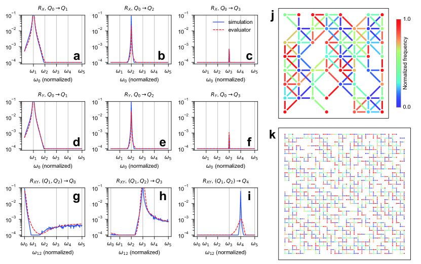
Figure 3: Demonstrations of the trained evaluator and designer. a-i. Some examples of fitted and simulated crosstalk errors between neighboring qubits in a linear graph with $6$ qubits numbered sequentially ’$Q_{0}-Q_{1}-Q_{2}-Q_{3}-Q_{4}-Q_{5}$’. The horizontal axes represent frequencies of nodes or edges where quantum operations are applied, and the vertical axes represent the corresponding crosstalk errors in logarithmic coordinates. The results of numerical simulation are plotted with the solid blue lines, while the outputs of the trained evaluator are depicted in the dashed red lines. The peaks of the blue or red lines represent the maximum errors. The gray vertical lines indicate the idling frequencies of the qubits. The fitted and simulated results agree well with each other, showcasing the effectiveness of the evaluator. j-k. Examples of the frequency assignments designed by the trained designer for a medium-scale graph and a large-scale graph. The node and edge colors correspond to the normalized node and edge frequencies. These figures demonstrate the designer’s effectiveness for considering nearest and higher-hop neighbors for both nodes and edges.

The evaluator. After generating the datasets through numerical simulations, the evaluator is trained, validated, and tested in a supervised learning manner. The evaluator consists of multiple MLPs. Each MLP serves for one type of quantum operations and predicts the average crosstalk excitation on a node $\mathcal{N}_{k}$ resulting from operations on node $\mathcal{N}_{i}$ (or edge $\mathcal{E}_{ij}$), where $k\neq i,j$. The inputs of the MLP are the relevant node and edge frequencies denoted by $\vec{\omega}$ and the distances represented by the elements of adjacency matrices, i.e., $A^{p}_{ik}$ (together with $A^{p}_{jk}$ for two-qubit operations). To maintain consistency in the outputs of the MLPs, the crosstalk errors in the simulated datasets are transformed using base-$10$ logarithms. Thus, the losses of the MLPs are determined by the corresponding MSEs, $\mathcal{L}_{O}^{\rm evaluator}=|\Lambda_{O}|^{-1}\sum_{\lambda\in\Lambda_{O}}\delta_{O,\lambda}^{2}$, and

$$\delta_{O,\lambda}=|{\rm MLP}_{O}(\vec{\omega}_{\lambda},A^{1}_{\lambda,ik},A^{2}_{\lambda,ik},\cdots)-{\rm log}_{10}(E_{O,\lambda})|,$$ (2)

where $O$ is the type of quantum operations, $\lambda$ is a specific index of data in the operation’s dataset $\Lambda_{O}$ with the size $|\Lambda_{O}|$, and $E_{O,\lambda}$ is the simulated crosstalk error. The crosstalk errors smaller than e.g., $1\times 10^{-4}$, or larger than, e.g., $1\times 10^{-1}$, are not concerned, because excessively small crosstalk errors usually do not dominate the error components, while larger ones exhibit strong randomness. Individual MLPs are supervisedly trained for different types of quantum operations, with the resulting MSEs and $r^{2}$ for the training, validation, extra validation, testing and extra testing sets presented in Tab. 1. The coefficient of determination $r^{2}$ exceeds $0.9$ for each case, indicating a strong ability of the evaluator to fit the dataset [53]. More details are available in the Methods section and the supplementary materials [43].

To demonstrate the reliability of the trained evaluator, we select various frequency assignments on a linear graph with $6$ qubits numbered sequentially ’$Q_{0}-Q_{1}-Q_{2}-Q_{3}-Q_{4}-Q_{5}$’, and compare the numerical simulation results with the fitting results from the evaluator. In Figs. 3(a)-(i), the solid blue lines describe the results from numerical simulations, while the dashed red lines represent the fitting results from the evaluator, and the two results agree well with each other. For single-qubit operations, we vary the node frequency $\omega_{0}$ of qubit $Q_{0}$ while maintaining the other frequencies constant. The crosstalk excitations on qubits $Q_{1},\,Q_{2}$ and $Q_{3}$ are plotted to signify the crosstalk errors induced by single-qubit operations. For two-qubit operations, we scan the edge frequency of coupled-qubit pair $(Q_{2},Q_{3})$ with the other frequencies unchanged, and plot the crosstalk excitations on qubits $Q_{1},\,Q_{4}$ and $Q_{5}$. It should be noted that minor discrepancies between the fitting results and the simulations are permissible, provided that the evaluator can guide the training of the designer.

The designer. As shown in Fig. 1, during the training of the designer, medium-scale graphs $\mathcal{G}=(\mathcal{N},\mathcal{E})$ with nodes $\mathcal{N}$ and edges $\mathcal{E}$ are randomly generated and input into the designer to output a frequency assignment $\vec{\omega}$ for each graph. The trained evaluator estimates the crosstalk errors for a particular $\vec{\omega}$ on corresponding $\mathcal{G}$. Then the designer’s loss could be calculated,

$$\mathcal{L}^{\rm designer}(\mathcal{G},\vec{\omega}) =\frac{1}{|\mathcal{N}|}\sum_{\mathcal{N}_{i}\in\mathcal{N}}\sum_{\mathcal{N}_{k}\neq\mathcal{N}_{i}}\hat{E}_{R_{X},\mathcal{N}_{i}\to\mathcal{N}_{k}}$$ (3)

$$+\frac{1}{|\mathcal{N}|}\sum_{\mathcal{N}_{i}\in\mathcal{N}}\sum_{\mathcal{N}_{k}\neq\mathcal{N}_{i}}\hat{E}_{R_{Y},\mathcal{N}_{i}\to\mathcal{N}_{k}}$$

$$+\frac{1}{|\mathcal{E}|}\sum_{\mathcal{E}_{i,j}\in\mathcal{E}}\sum_{\mathcal{N}_{k}\neq\mathcal{N}_{i},\mathcal{N}_{j}}\hat{E}_{R_{XY},\mathcal{E}_{ij}\to\mathcal{N}_{k}}.$$

First, the estimated crosstalk errors, e.g., $\hat{E}_{R_{X},\mathcal{N}_{i}\to\mathcal{N}_{k}}$, on different nodes $\mathcal{N}_{k}$ are summed to obtain the total crosstalk error of operations on node $\mathcal{N}_{i}$ (or edge $\mathcal{E}_{ij}$). Second, the node(edge)-related errors are subsequently averaged to get the errors for one specific type of quantum operations. Then, the crosstalk errors of all three types of quantum operations are summed up to obtain the comprehensive quantum crosstalk error, serving as the loss function $\mathcal{L}^{\rm designer}(\mathcal{G},\vec{\omega})$ under the specific graph $\mathcal{G}$ and frequency assignment $\vec{\omega}$. Finally, a batch of crosstalk errors for different graphs, together with the parameter assignment on each graph, i.e., $(\mathcal{G},\vec{\omega})$, are averaged to calculate the total loss for unsupervisedly training the designer. In our simulation, only the crosstalk errors up to 4-hop neighbors are taken into account, as the crosstalk errors diminish with distance as shown in Fig. 2(b). More details are given in the Methods section and the supplementary materials [43].

The randomly-generated training graphs contain around $54$, $103$ and $218$ nodes, and the training batch size is $288$ [54]. Approximately 700,000 training epochs were executed for about $2$ days with an RTX $4090$ GPU. Both node and edge frequencies are encompassed throughout the entire training. Validation is unnecessary because new random graphs are continuously generated throughout the unsupervised training process. Ultimately, the comprehensive crosstalk errors for all three types of quantum operations reach satisfactory levels. Figs. 3(j) and (k) show the parameter assignments output by the trained designer for medium- and large-scale graphs. These figures demonstrate the effectiveness of considering nearest and multi-hop neighbors for both nodes and edges, ensuring that their frequencies are as distinct as possible.

The trained designer can be readily applied to graphs of different structures and scales. The batched utilization strategy, as previously mentioned, can further enhance the designer’s effectiveness. We tested totally $30\times 6$ random graphs with average qubit numbers of $32$, $54$, $103$, $218$, $450$, and $870$, which utilize batch sizes of $512$, $512$, $512$, $64$, $8$, and $2$, respectively. Besides the GNNs-based designer, other methods were also tested for comparisons, including the direct application of a gradient-free optimizer, the direct utilization of gradient descent, and the Snake algorithm. We note that the trained evaluator is also necessary for the traditional methods, because conducting real experiments would require significant time and resources [26], and numerical simulation for SQECs with more than $20$ qubits is also challenging [24]. Further details about other methods can be found in the Methods section and supplementary materials [43]. The effectiveness and efficiency of all the four methods for different graph scales are shown in Fig. 4. All four methods employ the same trained evaluator on the same i9-14900KF CPU. Fig. 4(a) demonstrates that the well-trained GNNs-based designer achieves lower crosstalk errors than all other methods for all the graph scales. Additionally, the GNNs-based designer is exponentially faster than all other methods for all given tasks, as illustrated in Fig. 4(b). Especially for large-scale graphs where direct optimizations are not feasible, the GNNs-based designer achieves slightly more than half the errors of the Snake algorithm in several seconds, while the Snake algorithm would take dozens of minutes.

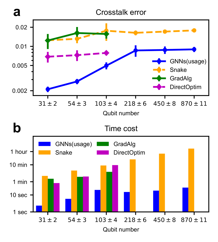
Figure 4: Effectiveness and efficiency. These are the detailed versions of Fig. 1(i). a. The average crosstalk errors using different methods on SQECs with various structures and scales. b. The real-world running times of different algorithms. In both a and b, the horizontal axes represent the averaged qubit numbers of the test graphs, ranging from medium to large scales. Here, we test the SQECs with average qubit numbers from $31$ to $870$. The vertical axes correspond to the error and time cost respectively. All axes are expressed in logarithmic coordinates. The application (usage) of our GNNs-based designer is depicted in blue, the Snake algorithm is in orange, the direct application of gradient descent algorithm is in green, and the direct utilization of a gradient-free optimization algorithm is in purple. All the tests are performed using the same CPU and the same evaluator. Only the GNNs-based designer and the Snake algorithm are available for the large-scale graphs. In these figures, the GNNs-based designer demonstrates advantages in terms of effectiveness, efficiency and scalability.

IV Discussions

We apply two graph-based neural-network models named evaluator and designer to tackle the challenge of mitigating quantum crosstalk errors in large-scale SQECs. The evaluator undergoes training, validation, and testing on three $6$-qubit graphs. Moreover, additional validation and testing are conducted on two extra $6$-qubit graphs to verify the evaluator’s generalization ability. Following the evaluator’s training, the designer is unsupervisedly trained on randomly generated medium-scale graphs, based on the errors estimated by the evaluator. The designer incorporates high-order graph convolutional networks, enables its direct applications to graphs of diverse structures and scales. According to our tests, the designer outperforms traditional optimization algorithms in both efficiency and effectiveness, particularly for large-scale SQECs. The proposed algorithm can be integrated with real experiments from two perspectives. On the one hand, the simulation data used to train the evaluator can also be collected through experiments. Even in cases where the experiment can only generate limited data, the MLPs in the evaluator can be substituted with simpler models that consider more theoretical insights. On the other hand, the parameter assignments provided by the designer can serve as initial optimization values which closely approximate the optimal experimental settings. In the future research, additional error sources and variations between qubits may be taken into account, thus the practicality of the proposed algorithm can be further enhanced.

The ’three-stair scaling’ mechanism harnesses the scaling benefits of graph neural networks, paves the way for EDA in the realm of large-scale SQECs. Considering the scaling challenge commonly exists in simulating large-scale quantum computing processors of different platforms which can also be abstracted into graph structures, the proposed algorithm could also be implemented on these platforms. Moreover, the concept of evaluating initially and optimizing subsequently could provide insights for applying neural networks into diverse problems in quantum computing.

V Data and Code Availability

The dataset generated by numerical simulations, the code for training, validating and testing the models, together with the trained models will be open-soured after the official publication of the paper.

VI Acknowledgments

We acknowledge J.-L. Long, Z. Wang, R.-B. Wu, G.-Z. Zhu, Y. Shang, T.-T. Chen, and G.-S. Liu for discussions. This work was support by Innovation Program for Quantum Science and Technology (Grant No. 2021ZD0300201).

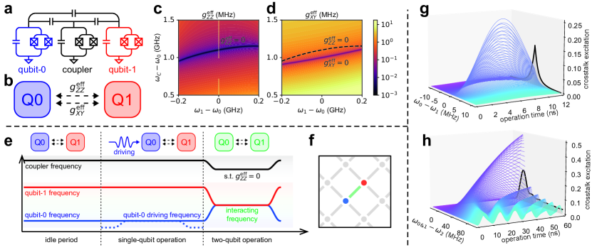
Figure 5: The physical system, quantum operations, and crosstalk analysis. a. The interconnected ’qubit-coupler-qubit’ subsystem as the building block of SQECs. b. Effective $ZZ$ and $XY$ couplings between the qubits, resulting in different types of quantum crosstalk. The coupler mode is equivalently eliminated. c. The variations of effective $ZZ$ coupling strength $g_{ZZ}^{\rm eff}$ as a function of the qubit and coupler frequencies. The dark line where $g_{ZZ}^{\rm eff}=0$ is referred to as the $ZZ$ free line. d. The variations of the effective $XY$ coupling strength $g_{XY}^{\rm eff}$ as a function of the qubit and coupler frequencies. The fitted $ZZ$-free line is depicted with the black dashed line. e. The control schemes and the corresponding frequency configurations for idle periods and different operations, where different frequencies are represented by different colors. In the idle period, the frequencies corresponding to the qubits and the coupler are $\omega_{0}$, $\omega_{1}$ and $\omega_{C}$, which are chosen to ensure that the effective couplings are negligibly small or minimized. For single-qubit operations on qubit $Q_{0}$, $Q_{0}$ is resonantly driven by external fields for a certain period of time (dashed blue line). For two-qubit operations, the qubit frequencies are adjusted to to enable resonant interaction for a specific duration. Meanwhile, the coupler frequency is adjusted to make $g_{ZZ}^{\rm eff}=0$, which may result in a non-zero value of $g_{XY}^{\rm eff}$. f. The graph-coloring representation of frequency assignments for a building block (blue and red dots connected by a green segment) of large-scale SQECs (lattice with the gray color). The node frequencies correspond to the qubit frequencies during the idle periods and single-qubit operations, and the edge frequencies denote the resonant frequencies that two qubits resonantly interact to realize two-qubit operations. g. The crosstalk excitations on qubit $Q_{1}$ when single-qubit operations are implemented on qubit $Q_{0}$ in building block of SQECs. h. The crosstalk excitations on qubit $Q_{2}$ when two-qubit operations are implemented on $Q_{0}$ and $Q_{1}$ in a system of three qubits with two couplers. Because operation times are related to the parameters given by the users, the errors are averaged over multiple operating times and depicted with the black lines. The peaks correspond to the maximum errors.

Appendix A Physical System

The building block of SQECs is the interconnected ’qubit-coupler-qubit’ subsystem [46] as schematically shown in Fig. 5(a), where three frequency-adjustable transmons [47] are capacitively coupled in pairs. The middle one functions as the tunable coupler, which is now extensively utilized in SQEC experiments, e.g. in Refs. [7, 8]. The building-block Hamiltonian of SQEC is

$$H= \sum_{i\in Q\cup C}\hbar\omega_{i}(t)a_{i}^{\dagger}a_{i}+\sum_{i\in Q\cup C}\hbar\frac{\alpha}{2}a_{i}^{\dagger}a_{i}\left(a_{i}^{\dagger}a_{i}-1\right)$$ (4)

$$+\sum_{i,j\in Q\cup C}\hbar g_{ij}\left(a_{i}^{\dagger}a_{j}+a_{i}a_{j}^{\dagger}\right)$$

$$+\sum_{i\in Q}\hbar\Omega_{i}^{x}(t)\cos[\omega_{di}^{x}(t)t]\left(a_{i}^{\dagger}+a_{i}\right)$$

$$-i\sum_{i\in Q}\hbar\Omega_{i}^{y}(t)\sin[\omega_{di}^{y}(t)t]\left(a_{i}^{\dagger}-a_{i}\right),$$

where $\hbar$ is the reduced Plank’s constant. The set $C$ only includes the middle transmon acting as the coupler, while the set $Q$ includes other two transmons as the qubits. $\omega_{i}(t)$ is the eigen-frequency of the first excitation, $a_{i}$ and $a^{\dagger}_{i}$ are the annihilation and creation operators of the $i$-th transmon, respectively. We assume that all three transmons have the same anharmonicity $\alpha$ for simplicity of discussions. The parameter $g_{ij}$ denotes the coupling strength between the $i$-th and the $j$-th transmons, $\omega_{di}^{x}(t)$ and $\omega_{di}^{y}(t)$ are the driving frequencies corresponding to the driving strengths $\Omega_{i}^{x}(t)$ and $\Omega_{i}^{y}(t)$ for different single-qubit operations [10]. We note that the time-dependent terms can be controlled or devised by the experimenters.

In this building block, the two qubits typically have the resonant or near resonant frequencies, while the middle coupler is often detuned significantly from two qubits. Thus, the coupler mode can be equivalently eliminated, leading to the weak effective $ZZ$ and $XY$ couplings between two qubits [33], as illustrated in Fig. 5(b). According to the definition [33, 55], the $ZZ$ coupling can be given as

$$g_{ZZ}^{\rm eff}\equiv(E_{\ket{110}}-E_{\ket{100}})-(E_{\ket{010}}-E_{\ket{000}}),$$ (5)

where $E_{\ket{Q0,Q1,C}}$ represents the energy corresponding to the state $\ket{Q0,Q1,C}$, in which qubit $Q_{0}$, qubit $Q_{1}$ and the coupler are in the states $|Q0\rangle$, $|Q1\rangle$ and $|C\rangle$, respectively. The variations of the effective $ZZ$ coupling strength $g_{ZZ}^{\rm eff}$ via the frequencies of the qubits and coupler can be numerically solved by diagonalizing the Hamiltonian without driving fields, as depicted in Fig. 5(c). By taking the Schrieffer-Wolff transformation [41], the effect of the coupler can also be equivalent to the effective $XY$ coupling,

$$g_{XY}^{\rm eff}=g_{QQ}-\frac{g_{QC}^{2}}{2}\left(\frac{1}{\omega_{C}-\omega_{0}}+\frac{1}{\omega_{C}-\omega_{1}}\right),$$ (6)

where $\omega_{0},\omega_{1},\omega_{C}$ are the frequencies of $Q_{0}$, $Q_{1}$ and coupler, $g_{QQ}$ is the direct coupling strength between two qubits, and $g_{QC}$ is the direct coupling strength between the qubits and the coupler. $g_{XY}^{\rm eff}$ is plotted in Fig. 5(d). The existence of non-zero $ZZ$ and $XY$ couplings results in different types of quantum crosstalk errors, however, as shown in Figs. 5(c) and (d), the non-simultaneous-zero values of the two couplings present a theoretical challenge in completely eliminating crosstalk errors between the two qubits. To address this challenge, we adjust $\omega_{C}$ to keep the system on the so-called $ZZ$-free line (i.e., $g_{ZZ}^{\rm eff}=0$) [33], aiming to eliminate the crosstalk errors induced by the $ZZ$ coupling. Consequently, qubit frequencies can be designed to mitigate crosstalk errors arising from the $XY$ coupling.

Appendix B Quantum Operations

Quantum crosstalk commonly arises during quantum operations, also called as quantum gates. We select single-qubit $R_{X}$, $R_{Y}$ [44], and two-qubit $R_{XY}$ operations [52] as the fundamental quantum gates. According to the quantum computation principles, these three types of operations can be combined to construct universal quantum computation [44]. Fig. 5(e) illustrates the control for the frequencies of qubits, coupler and driving fields across idle periods, single-qubit operations, and two-qubit operations. Here, the idle periods denote that no quantum operations are applied [33].

1. During idle periods, $\omega_{0}$ and $\omega_{1}$ are carefully assigned to minimize crosstalk errors arising from the effective $XY$ coupling, while $\omega_{C}$ is positioned on the $ZZ$-free line to ensure that crosstalk errors induced by the effective $ZZ$ coupling are eliminated.

2. When operating a single-qubit operation on qubit $Q_{0}$, the frequencies $\omega_{0}$, $\omega_{1}$ and $\omega_{C}$ remain unchanged, while a resonant driving field with $\omega_{0d}=\omega_{0}$ is applied to $Q_{0}$, as denoted by the blue dashed line in Fig. 5(e). By regulating the intensity, duration, and polarization direction (e.g., $X$ or $Y$) of the driving field, a specific single-qubit operation on $Q_{0}$ can be achieved.

3. During a two-qubit operation involving $Q_{0}$ and $Q_{1}$, both qubits are adjusted to have the same frequency, resonantly interact for a specific duration to realize a specific operation. Simultaneously, $\omega_{C}$ is adjusted in synchronization to ensure that the system consistently operates on the $ZZ$-free line.

Fig. 5(f) shows the corresponding graph-coloring [29, 30] representation of the frequency assignment, where the frequencies are normalized and represented by different colors. The node frequencies correspond to the qubit frequencies during the idle periods and single-qubit operations, and the edge frequencies denote the resonant frequencies that two qubits resonantly interact to realize two-qubit operations. Both node and edge frequencies constitute the parameters to be designed by the algorithm proposed in this study.

Appendix C Crosstalk Analysis

In order to quantitatively describe quantum crosstalk, the undesired excitations occurring on a specific qubit $Q_{k}$ are simulated when single-qubit (or two-qubit) operations are applied to qubit $Q_{i}$ (or coupled-qubit pair $Q_{i}\&Q_{j}$) with $k\neq i,j$. We define such excitations on $Q_{k}$ as crosstalk errors from node $\mathcal{N}_{i}$ (or edge $\mathcal{E}_{ij}$) to node $\mathcal{N}_{k}$. In our simulations, $Q_{i}$ is (or $Q_{i}\&Q_{j}$ are) initialized to some excited states, while $Q_{k}$ is set in its ground state. After finishing the simulation, the average excitation on $Q_{k}$ is calculated to reflect the crosstalk error under the corresponding configurations.

For a given type of quantum operations, the main factors influencing crosstalk errors include the qubit frequencies, the qubit distances within the graph, the inter-qubit coupling strengths, the driving strengths of single-qubit operations, and the time durations of operations.

1. Qubit frequencies: Qualitatively, because the conservation of both energy and excitation number must be satisfied simultaneously, the quantum crosstalk error between two qubits is expected to increase as their frequency difference decreases [43]. As shown in the black lines in Figs. 5(g) and (h), the correlations between nearest-neighbor crosstalk errors and frequency differences are evident, which facilitates the fitting with neural networks.

2. Qubit distances within the graph: Given that the distant qubits can only interact through weak indirect or parasitic couplings [45], the quantum crosstalk error between them would significantly decrease with the increase of their distance, as exemplified in Fig. 2(b). Qubit distances are also taken into account by the evaluator to estimate quantum crosstalk errors.

3. Coupling and driving strengths: The coupling strengths between two qubits (or between a qubit and a coupler) and the driving strengths for single-qubit operations can also influence quantum crosstalk errors. The decrease of the coupling and driving strengths generally helps to mitigate crosstalk errors, but this often impacts the efficiency of quantum operations [33]. Moreover, the trade-off and adjustment of coupling and driving strengths are independent on the graph structure, thus their values are fixed in this study.

4. Time durations of operations: As demonstrated in Figs. 5(g) and (h), time durations could affect crosstalk excitations when single- or two-qubit operations are implemented. Nevertheless, when other parameters are given, the time duration for a specific operation is determined by the user-input parameters, such as the rotation angle of $R_{X}$ gate. Therefore, crosstalk errors are averaged over multiple time durations in our numerical simulations.

In this work, classical resources of errors are not considered. For example, defects in fabrication [56] and distortions in modulating microwave pulses [57] can also affect the quality of quantum information processing. Additionally, when signals are applied through specific control lines, the microwave current induced magnetic fields may introduce unwanted signals in other control lines, leading to what is known as classical crosstalk. Many works are studying the mitigation of classical crosstalk errors [58, 59, 60]. The classical resources of errors are not taken into account in this study, because they are usually graph-independent.

In a word, after the coupling and driving strengths are given and multiple operating time durations are averaged, the quantum crosstalk errors only depend on the node and edge frequencies, graph structures, and operation types. Thus, neural networks can be trained to evaluate the frequency assignments for quantum crosstalk mitigation.

Appendix D Numerical Simulations

To simulate quantum operations, the Hamiltonian in Eq. (4) is transformed into a rotating frame with the rotating wave approximations [61]. Taking the single-qubit $R_{X}$ operation applying on qubit $Q_{0}$ as an example, the transformed Hamiltonian without other operations in Eq. (4) is given as

$$\tilde{H}= \sum_{i\in Q\cup C}\hbar(\omega_{i}-\omega_{0})a_{i}^{\dagger}a_{i}+\sum_{i\in Q\cup C}\hbar\frac{\alpha}{2}a_{i}^{\dagger}a_{i}\left(a_{i}^{\dagger}a_{i}-1\right)$$ (7)

$$+\sum_{i,j\in Q\cup C}\hbar g_{ij}\left(a_{i}^{\dagger}a_{j}+a_{i}a_{j}^{\dagger}\right)+\hbar\frac{\Omega_{0}^{x}}{2}\left(a_{0}^{\dagger}+a_{0}\right),$$

which can be numerically solved to obtain an expected quantum operation. We note that all quantum states involved in numerical simulations for quantum operations are dressed states [42], which can be directly measured in real experiments.

In our simulations, the adjustable qubit frequencies are assumed to be in the range of $4.9$ to $5.1$ GHz. The coupler frequencies are aligned along the $ZZ$-free line, which are around $6.0$ GHz. Other parameters are assumed as follows. The anharmonicity of each qubit and coupler are $300$ MHz. The direct qubit-qubit coupling is $10$ MHz, the qubit-coupler coupling is $100$ MHz, the single-qubit driving strength is $25$ MHz, and the driving frequency matches the corresponding qubit frequency. Residual coupling between higher-order neighboring qubits due to parasitic capacitance is also taken into account [33, 45], which is $0.1$ MHz between $2$-hop neighboring qubits and $0.01$ MHz between $3$-hop neighboring qubits.

According to the definition, the quantum crosstalk errors from node $\mathcal{N}_{i}$ (or edge $\mathcal{E}_{ij}$) to node $\mathcal{N}_{k}$ are simulated. When focusing on the single-qubit operations on qubit $Q_{i}$, and taking $R_{X}$ operations as an example, we assume that the quantum state of $Q_{i}$ is initialized to $\ket{\pm}_{i}=\left(\ket{0}_{i}+\ket{1}_{i}\right)/\sqrt{2}$, while the other qubits are initialized to their ground states. In our simulations, $20$ operation time durations are uniformly sampled in a range from $0$ to $2\pi/\Omega^{x}$, corresponding to rotating angles of $R_{X}$ operations uniformly sampled from $0$ to $2\pi$. Thus, the undesired excitations on qubit $Q_{k}$ across these $40$ scenarios are simulated and averaged to represent the crosstalk error from $Q_{i}$ to $Q_{k}$ when $R_{X}$ operations are implemented. For two-qubit operations applied to the coupled-qubit pair $(Q_{i},Q_{j})$, the initial states are assumed to be $\ket{+}_{i}\ket{+}_{j}$ or $\ket{-}_{i}\ket{-}_{j}$, with the remaining qubits in their ground states. In our simulations, $20$ time durations ranging from $0$ to $2\pi/g_{XY}^{\rm eff}$ are also uniformly sampled. Similar to the approach taken for single-qubit operations, $40$ crosstalk excitations from coupled-qubit pair $(Q_{i},Q_{j})$ to $Q_{k}$ are simulated and averaged.

The dataset used for training, validating, and testing the evaluator is generated on small graphs as shown in Fig. 2(a), which are the most common qubit coupling structures. Specifically, $25,600$ sets of node and edge frequencies are randomly sampled on the $6$-qubit graphs in the left of Fig. 2(a), and the corresponding crosstalk errors are simulated. The dataset is divided into training, validation, and testing sets at an $8:1:1$ ratio. To ensure the generalization ability of the trained evaluator, additional simulations are conducted on the two extra $6$-qubit graphs illustrated in the right of Fig. 2(a), producing the datasets only for validation and testing. Notice that the evaluator is also applicable for simultaneous operations, see supplementary materials for details [43].

Appendix E Evaluator: Graph-Based MLPs

The evaluator comprises multiple MLPs to estimate the errors associated with different types of quantum operations. Each MLP is tailored to a specific type of quantum operations, such as $R_{X}$, $R_{Y}$, or $R_{XY}$ operations. These MLPs are trained to output the base-$10$ logarithm of respective crosstalk errors, while the inputs for single- and two-qubit operations are slightly different. The MLPs for single-qubit operations are trained to predict the undesired excitations from one node to another. Taking the average crosstalk error of $R_{X}$ operation from node $\mathcal{N}_{i}$ to node $\mathcal{N}_{k}$ as an example, the MLP takes the node frequencies $\omega_{i},\omega_{k}$ and the corresponding matrix elements $(A^{p})_{ik}$ as inputs, where $(A^{p})_{ik}$ denotes the element of the $p$-th order adjacency matrix as defined before. The MLP for two-qubit $R_{XY}$ operations can evaluate the crosstalk error from edge $\mathcal{E}_{ij}$ to node $\mathcal{N}_{k}$, where $k\neq i,j$. Similar to the case of single-qubit operations, the inputs for two-qubit operations encompass the node frequencies $\omega_{i},\omega_{j},\omega_{k}$, the edge frequency $\omega_{ij}$, as well as the matrix elements $(A^{p})_{ik}$ and $(A^{p})_{jk}$. Each MLP comprises $4$ hidden layers, each with $32$ neurons. Further details can be found in the supplementary materials [43].

Appendix F Designer: GNNs and MLPs

As shown in Fig. 2(d), the designer is used to design parameters on both nodes and edges within the input graphs. Given a batch of graphs and random node frequencies as inputs, a deep high-order GCN and an MLP can assign frequencies for each node, which constitute part of the designer’s output. Subsequently, these node frequencies serve as inputs for another high-order GCN to output new node features, which are then aggregated by edges and fed into an MLP. For an edge $\mathcal{E}_{ij}$, with a softmax function applied to the two output-layer neurons, the MLP generates the selection preferences $p_{i}$ and $p_{j}$ for the respective edge frequency $\omega_{ij}$ from its two node frequencies $\omega_{i}$ and $\omega_{j}$. Ultimately, each edge’s frequency is determined by

$$\omega_{ij}=p_{i}\omega_{i}+p_{j}\omega_{j}.$$ (8)

Thus another part of the designer’s output is obtained. In this work, the three-order GCN for node frequencies comprises $12$ hidden layers, and contains $256$ neurons for most of the layers. While the three-order GCN for edge frequencies consists of $3$ hidden layers, each with $64$ neurons. As a comparison, the training effects and model sizes of standard GCN and different high-order GCNs are plotted in Fig. 6. High-order GCNs perform much better than the standard one, demonstrating the necessity of introducing high-order GCNs. Three-order GCN is used in the designer because the relevant errors mainly relate to the nearest neighboring, $2$-hop neighboring and $3$-hop neighboring qubits, as shown in Fig. 2(b). More details are available in the supplementary materials [43].

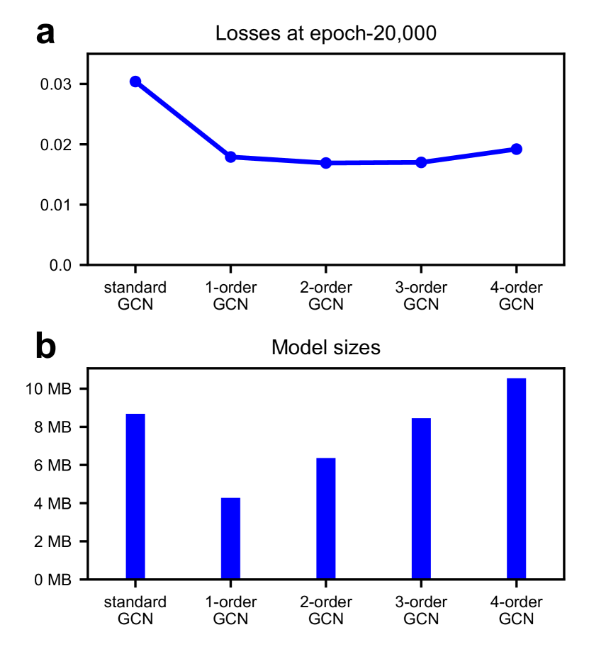
Figure 6: Comparison between standard and high-order GCNs. a. The training losses at the $20,000$-th epoch. b. The model sizes of compared GCNs. High-order GCNs perform much better than standard GCN with similar model sizes. This comparison demonstrates the necessity of introducing high-order GCNs, rather than simply using standard GCN. In this study, three-order GCN is used because the dominant errors only relate to the nearest neighboring, $2$-hop neighboring and $3$-hop neighboring qubits, as shown in Fig. 2(b).

Appendix G Traditional Methods

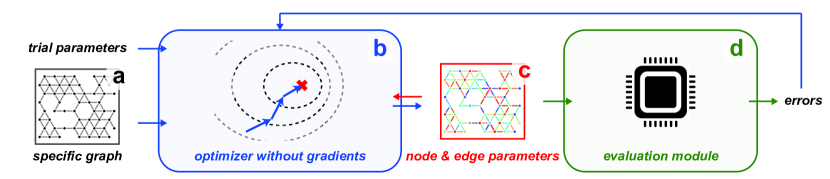
Figure 7: Direct optimization algorithms. For a specific graph, randomly generated trial parameters for all the nodes and edges are input into the optimizer. The optimizer iteratively explores new parameter assignments, gives them to the evaluation module for evaluating the corresponding errors, and then feeds these errors back to ultimately obtain an appropriate parameter assignment. a. An example of the specific graph. b. The gradient-free optimizer. c. Node and edge parameters designed for the input graph. d. The evaluation module, e.g., real experiments for small-scale SQECs, or the trained evaluator for larger SQECs.

In addition to the GNNs-based designing algorithm proposed in this study, three traditional methods are also discussed for comparisons. These include the direct utilization of a gradient-free optimization algorithm (DirectOptim), the direct application of gradient descent algorithm (GradAlg), and the Snake algorithm for large-scale graphs [25, 26].

1. DirectOptim: A straightforward consideration for the parameter designing problem is to utilize feedback-based optimization algorithms [62] to find available parameter assignments for specific coupled-qubit graphs directly, as shown in Fig. 7. For a specific graph as exemplified in Fig. 7(a), randomly generated trial parameters for all the nodes and edges are input into the optimizer. The optimizer, shown in Fig. 7(b), iteratively explores new parameter assignments, such as Fig. 7(c). In Fig. 7(d), the assignments are given to the evaluation module to assess the corresponding errors. The evaluation module can utilize real experiments for small-scale SQECs or employ the trained evaluator for larger-scale SQECs. Then the errors are fed back to the optimizer to ultimately obtain an appropriate parameter assignment.

2. GradAlg: The direct application of gradient descent algorithm is similar to DirectOptim, which replaces the gradient-free optimizers in DirectOptim with gradient descent algorithms. Since the errors under given frequency assignments can be estimated through the evaluator, the corresponding gradient information is available after the errors are calculated. So, gradient descent algorithms can be utilized to find the frequency assignments with mitigated errors.

3. Snake: Due to the low computational efficiency, DirectOptim and GradAlg are not applicable for large-scale SQECs. Snake algorithm was proposed as an improvement of direct optimization by dividing the entire graph into multiple small-scale subgraphs and sequentially applying the optimizer to optimize these subgraphs [25, 26]. Thus, Snake algorithm can be used to design parameters for larger-scale graphs, such as the Sycamore processor, which is said to be the first to achieve quantum supremacy [7].

All these traditional algorithms overlook the graph structures established by the qubits and their couplings. This oversight may significantly impact the effectiveness and efficiency of optimization when considering large-scale graphs.

In our tests, both GNNs-based designing algorithm and the three traditional algorithms leverage the trained evaluator to estimate the crosstalk errors. For Snake and DirectOptim, Powell optimizer is employed [63], and all other settings adhere to the default settings provided by Scipy [62]. The scope of Snake is $4$, which is the best choice in Ref. [26]. Among these four algorithms, the GNNs-based designer and Snake are available for large-scale graphs, whereas the other two are limited to medium-scale graphs due to their inefficiency. On the other hand, the GNNs-based designer and GradAlg require gradient information from the evaluator, while the other methods can use gradient-free optimizers. Following a prolonged training phase, the GNNs-based designer can be swiftly applied to graphs of varying structures and scales. In contrast, the traditional methods necessitate distinct optimization for each specific graph with relatively slower processing speeds.

References

- [1] Shor, P. W. Algorithms for quantum computation: discrete logarithms and factoring. In Proc. 35th annual symposium on foundations of computer science (IEEE, 1994).
- [2] Grover, L. K. A fast quantum mechanical algorithm for database search. In Proc. 28th Annual ACM Symposium on Teory of Computing, 212-219 (Association for Computing Machinery, 1996).
- [3] McArdle, S., Endo, S., Aspuru-Guzik, A., Benjamin, S. C., & Yuan, X. Quantum computational chemistry. Rev. Mod. Phys. 92, 015003 (2020).
- [4] Biamonte, J., Wittek, P., Pancotti, N., Rebentrost, P., Wiebe, N., & Lloyd, S. Quantum machine learning. Nature 549, 195-202 (2017).
- [5] Bluvstein, D., Evered, S. J., Geim, A. A., Li, S. H., Zhou, H., Manovitz, T., … & Lukin, M. D. Logical quantum processor based on reconfigurable atom arrays. Nature 626, 58-65 (2024).
- [6] Pogorelov, I., Feldker, T., Marciniak, C. D., Postler, L., Jacob, G., Krieglsteiner, O., … & Monz, T. Compact ion-trap quantum computing demonstrator. PRX Quantum 2, 020343 (2021).
- [7] Arute, F., Arya, K., Babbush, R., Bacon, D., Bardin, J. C., Barends, R., … & Martinis, J. M. Quantum supremacy using a programmable superconducting processor. Nature 574, 505-510 (2019).
- [8] Wu, Y., Bao, W. S., Cao, S., Chen, F., Chen, M. C., Chen, X., … & Pan, J. W. Strong quantum computational advantage using a superconducting quantum processor. Phys. Rev. Lett. 127, 180501 (2021).
- [9] Kim, Y., Eddins, A., Anand, S., Wei, K. X., Van Den Berg, E., Rosenblatt, S., … & Kandala, A. Evidence for the utility of quantum computing before fault tolerance. Nature 618, 500-505 (2023).
- [10] Gu, X., Kockum, A., Miranowicz, A., Liu, Y. & Nori, F. Microwave photonics with superconducting quantum circuits. Phys. Rep. 718, 1-102 (2017).
- [11] Castelvecchi, Davide. IBM releases first-ever 1,000-qubit quantum chip. Nature 624, 238-238 (2023).
- [12] Khammassi, N., Ashraf, I., Fu, X., Almudever, C. G., & Bertels, K. QX: A high-performance quantum computer simulation platform. in Design, Automation & Test in Europe Conference & Exhibition (DATE) 2017 (IEEE, 2017).
- [13] Cincio, L., Rudinger, K., Sarovar, M., & Coles, P. J. Machine learning of noise-resilient quantum circuits. PRX Quantum 2, 010324 (2021).
- [14] Convy, I., Liao, H., Zhang, S., Patel, S., Livingston, W. P., Nguyen, H. N., … & Whaley, K. B. Machine learning for continuous quantum error correction on superconducting qubits. New J. Phys. 24, 063019 (2022).
- [15] LeCompte, T., Qi, F., Yuan, X., Tzeng, N. F., Najafi, M. H., & Peng, L. Machine learning-based qubit allocation for error reduction in quantum circuits. IEEE Transactions on Quantum Engineering (2023).
- [16] Fürrutter, F., Muñoz-Gil, G., & Briegel, H. J. Quantum circuit synthesis with diffusion models. Nature Machine Intelligence 6, 515-524 (2024).
- [17] Dong, D., Chen, C., Qi, B., Petersen, I. R., & Nori, F. Robust manipulation of superconducting qubits in the presence of fluctuations. Scientific Reports, 5, 7873 (2015).
- [18] Bukov, M., Day, A. G., Sels, D., Weinberg, P., Polkovnikov, A., & Mehta, P. Reinforcement learning in different phases of quantum control. Phys. Rev. X 8, 031086 (2018).
- [19] Baum, Y., Amico, M., Howell, S., Hush, M., Liuzzi, M., Mundada, P., … & Biercuk, M. J. Experimental deep reinforcement learning for error-robust gate-set design on a superconducting quantum computer. PRX Quantum 2, 040324 (2021).
- [20] Wang, L. T., Chang, Y. W., & Cheng, K. T. T., eds. Electronic design automation: synthesis, verification, and test. Morgan Kaufmann, 2009.
- [21] Huang, G., Hu, J., He, Y., Liu, J., Ma, M., Shen, Z., … & Wang, Y. Machine learning for electronic design automation: A survey. ACM Transactions on Design Automation of Electronic Systems (TODAES) 26, 1-46 (2021).
- [22] Lopera, D. S., Servadei, L., Kiprit, G. N., Hazra, S., Wille, R., & Ecker, W. A survey of graph neural networks for electronic design automation. 2021 ACM/IEEE 3rd Workshop on Machine Learning for CAD (MLCAD) (IEEE, 2021).
- [23] Mirhoseini, A., Goldie, A., Yazgan, M., Jiang, J. W., Songhori, E., Wang, S., … & Dean, J. A graph placement methodology for fast chip design. Nature 594, 207-212 (2021).
- [24] For a quantum system with quantum modes including qubits or couplers, the dimension of Hilbert space is if only two quantum states are considered for every mode. For example, a system containing qubits need float numbers for simulation, which requires a memory of about TB.
- [25] Klimov, P. V., Kelly, J., Martinis, J. M., & Neven, H. The snake optimizer for learning quantum processor control parameters. Preprint at arXiv: 2006.04594 (2020).
- [26] Klimov, P. V., Bengtsson, A., Quintana, C., Bourassa, A., Hong, S., Dunsworth, A., … & Neven, H. Optimizing quantum gates towards the scale of logical qubits. Nature Communications 15, 2442 (2024).
- [27] Kipf, Thomas N., & Max Welling. Semi-supervised classification with graph convolutional networks. In International Conference on Learning Representations (2017).
- [28] Veličković, P., Cucurull, G., Casanova, A., Romero, A., Lio, P., & Bengio, Y. Graph attention networks. In International Conference on Learning Representations (2018).
- [29] Lemos, H., Prates, M., Avelar, P., & Lamb, L. Graph colouring meets deep learning: efective graph neural network models for combinatorial problems. In 2019 IEEE 31st International Conference on Tools with Artifcial Intelligence (ICTAI) (IEEE, 2019).
- [30] Schuetz, M. J., Brubaker, J. K., Zhu, Z., & Katzgraber, H. G. Graph coloring with physics-inspired graph neural networks. Phys. Rev. Research 4, 043131 (2022).
- [31] Rosenblatt, Frank. The perceptron: a probabilistic model for information storage and organization in the brain. Psychological Review 65, 386-408 (1958).
- [32] Rumelhart, D. E., Hinton, G. E., & Williams, R. J. Learning representations by back-propagating errors. Nature 323, 533-536 (1986).
- [33] Zhao, P., Linghu, K., Li, Z., Xu, P., Wang, R., Xue, G., … & Yu, H. Quantum crosstalk analysis for simultaneous gate operations on superconducting qubits. PRX Quantum 3, 020301 (2022).
- [34] Harper, R., Flammia, S. T., & Wallman, J. J. Efficient learning of quantum noise. Nature Physics 16, 1184-1188 (2020).
- [35] Osman, A., Fernández-Pendás, J., Warren, C., Kosen, S., Scigliuzzo, M., Frisk Kockum, A., … & Bylander, J. Mitigation of frequency collisions in superconducting quantum processors. Phys. Rev. Research 5, 043001 (2023).
- [36] Ding, Y., Gokhale, P., Lin, S. F., Rines, R., Propson, T., & Chong, F. T. Systematic crosstalk mitigation for superconducting qubits via frequency-aware compilation. 2020 53rd Annual IEEE/ACM International Symposium on Microarchitecture (MICRO) (IEEE, 2020).
- [37] Tripathi, V., Chen, H., Khezri, M., Yip, K. W., Levenson-Falk, E. M., & Lidar, D. A. Suppression of crosstalk in superconducting qubits using dynamical decoupling. Phys. Rev. Applied 18, 024068 (2022).
- [38] Mundada, P., Zhang, G., Hazard, T., & Houck, A. Suppression of qubit crosstalk in a tunable coupling superconducting circuit. Phys. Rev. Applied 12, 054023 (2019).
- [39] Zhou, Z., Sitler, R., Oda, Y., Schultz, K., & Quiroz, G. Quantum crosstalk robust quantum control. Phys. Rev. Lett. 131, 210802 (2023).
- [40] Xie, L., Zhai, J., Zhang, Z., Allcock, J., Zhang, S., & Zheng, Y. C. Suppressing crosstalk of quantum computers through pulse and scheduling co-optimization. In Proceedings of the 27th ACM International Conference on Architectural Support for Programming Languages and Operating Systems (2022).
- [41] Schrieffer, J. R., & Wolff, P. A. Relation between the anderson and kondo hamiltonians. Phys. Rev. 149, 491 (1966).
- [42] Timoney, N., Baumgart, I., Johanning, M., Varón, A. F., Plenio, M. B., Retzker, A., & Wunderlich, C. Quantum gates and memory using microwave-dressed states. Nature 476, 185-188 (2011).
- [43] See Supplementary Materials.
- [44] Nielsen, M. A., & Chuang, I. L. (2010). Quantum computation and quantum information. Cambridge university press.
- [45] Zhao, P., Xu, P., Lan, D., Tan, X., Yu, H., & Yu, Y. Switchable next-nearest-neighbor coupling for controlled two-qubit operations. Phys. Rev. Applied 14, 064016 (2020).
- [46] Yan, F., Krantz, P., Sung, Y., Kjaergaard, M., Campbell, D. L., Orlando, T. P., … & Oliver, W. D. Tunable coupling scheme for implementing high-fidelity two-qubit gates. Phys. Rev. Applied 10, 054062 (2018).
- [47] Koch, J., Yu, T. M., Gambetta, J., Houck, A. A., Schuster, D. I., Majer, J., … & Schoelkopf, R. J. Charge-insensitive qubit design derived from the Cooper pair box. Phys. Rev. A 76, 042319 (2007).
- [48] Paszke, A., Gross, S., Massa, F., Lerer, A., Bradbury, J., Chanan, G., … & Chintala, S. Pytorch: An imperative style, high-performance deep learning library. Advances in neural information processing systems (2019).
- [49] Abadi, M., Barham, P., Chen, J., Chen, Z., Davis, A., Dean, J., … & Zheng, X. {TensorFlow}: a system for {Large-Scale} machine learning. 12th USENIX symposium on operating systems design and implementation (OSDI 16) (2016).
- [50] Liu, S., Chen, L., Dong, H., Wang, Z., Wu, D., & Huang, Z. Higher-order Weighted Graph Convolutional Networks. Preprint at arXiv: 1911.04129 (2019).
- [51] Kang, Y., Chen, J., Cao, Y., & Xu, Z. A higher-order graph convolutional network for location recommendation of an air-quality-monitoring station. Remote Sens. 13, 1600 (2021).
- [52] Schuch, N., & Siewert, J. Natural two-qubit gate for quantum computation using the interaction. Phys. Rev. A 67, 032301 (2003)
- [53] Wright, Sewall. Correlation and causation. Journal of agricultural research 20 557 (1921).
- [54] For a batch of graphs, there are 32 random graphs for each of the three fundamental graphs in Fig. 1(f) and each of the three scales, so the total batch size is .
- [55] Zhao, P., Xu, P., Lan, D., Chu, J., Tan, X., Yu, H., & Yu, Y. High-contrast zz interaction using superconducting qubits with opposite-sign anharmonicity. Physical review letters, 125, 200503 (2020).
- [56] De Leon, N. P., Itoh, K. M., Kim, D., Mehta, K. K., Northup, T. E., Paik, H., … & Steuerman, D. W. Materials challenges and opportunities for quantum computing hardware. Science 372, 6539 (2021).
- [57] Martinis, J. M., & Geller, M. R. Fast adiabatic qubit gates using only control. Phys. Rev. A 90, 022307 (2014).
- [58] Dai, X., Tennant, D. M., Trappen, R., Martinez, A. J., Melanson, D., Yurtalan, M. A., … & Lupascu, A. Calibration of flux crosstalk in large-scale flux-tunable superconducting quantum circuits. PRX Quantum 2, 040313 (2021).
- [59] Spring, P. A., Tsunoda, T., Vlastakis, B., & Leek, P. J. Modeling enclosures for large-scale superconducting quantum circuits. Phys. Rev. Applied 14, 024061 (2020).
- [60] Yang, X. Y., Zhang, H. F., Du, L., Tao, H. R., Guo, L. L., Wang, T. L., … & Guo, G. P. Fast, universal scheme for calibrating microwave crosstalk in superconducting circuits. Appl. Phys. Lett. 125, 044001 (2024).
- [61] Twyeffort Irish, E. K. Generalized rotating-wave approximation for arbitrarily large coupling. Phys. Rev. Lett. 99, 173601 (2007).
- [62] Virtanen, P., Gommers, R., Oliphant, T. E., Haberland, M., Reddy, T., Cournapeau, D., … & Van Mulbregt, P. SciPy 1.0: fundamental algorithms for scientific computing in Python. Nature Methods 17, 261-272 (2020).
- [63] Powell, M. J. An efficient method for finding the minimum of a function of several variables without calculating derivatives. The computer journal, 7, 155-162 (1964).