Extracting Linear Relations from Gröbner Bases for Formal Verification of And-Inverter Graphs

Abstract

Formal verification techniques based on computer algebra have proven highly effective for circuit verification. The circuit, given as an and-inverter graph, is encoded as a set of polynomials that automatically generates a Gröbner basis with respect to a lexicographic term ordering. Correctness of the circuit can be derived by computing the polynomial remainder of the specification. However, the main obstacle is the monomial blow-up during the rewriting of the specification, which leads to the development of dedicated heuristics to overcome this issue.

In this paper, we investigate an orthogonal approach and focus the computational effort on rewriting the Gröbner basis itself. Our goal is to ensure the basis contains linear polynomials that can be effectively used to rewrite the linearized specification. We first prove the soundness and completeness of this technique and then demonstrate its practical application. Our implementation of this method shows promising results on benchmarks related to multiplier verification.

1 Introduction

Formal verification techniques based on algebraic reasoning have emerged as highly effective tools for verifying hardware, particularly in the context of verifying arithmetic circuits on the gate-level. As digital systems become more complex, ensuring the correctness of such circuits is paramount, especially in safety-critical applications like cryptography and signal processing to prevent a repetition of infamous failures, such as the Pentium FDIV bug [28]. Established methods based on satisfiability solving (SAT) [4], or binary decision diagrams (BDDs) [7] often struggle with the complex non-linear structure of arithmetic circuits. In contrast, formal verification techniques based on theorem provers [29] or computer algebra, specifically those leveraging Gröbner bases, offer an effective alternative and have made significant progress in recent years [18, 16, 26, 19].

In the algebraic method, the circuit is given as an and-inverter graph (AIG) [20]. The graph is encoded as a set of polynomials, which are sorted according to a lexicographic term ordering, where for each gate in the circuit the output variable is always greater than the input variables of the gate. Hence, the leading terms of the polynomial equations consist of single variables that are mutually disjoint. This property was called unique monic leading term (UMLT) in [16].

If such an ordering is chosen, the polynomials automatically form a Gröbner basis [5]. Informally said, a Gröbner basis is a mathematical construct that offers a decision procedure that guarantees soundness and completeness of the verification process. The correctness of the circuit is determined by computing the unique polynomial remainder of the specification polynomial, which represents the intended functionality of the circuit, modulo the Gröbner basis. The circuit fulfills the specification if and only if the final remainder is zero [17].

However, a major practical obstacle in using a lexicographic term ordering is the significant computational effort during the rewriting process, as the degree is not bounded. The size and degree of the intermediate reduction results typically increases tremendously, which is often deferred to as monomial blow-up [25]. Without specialized heuristics or preprocessing, the computation of the remainder often fails due to the rapid growth of the intermediate reduction results. To address this challenge, various preprocessing and rewriting algorithms have been developed, which syntactically or semantically analyze the input circuit to remove redundant information from the polynomial encoding, ultimately optimizing the reduction process and improving the efficiency of the verification.

Related Work.

Advanced reduction engines designed for the automatic algebraic verification of multipliers given as AIGs are implemented in tools such as DynPhaseOrderOpt [18], DyPoSub [26], and AMulet2 [16, 15], including its variant TeluMA [14]. In [16] and the corresponding tool AMulet2 [15] the authors employ SAT solving to rewrite certain parts of the multiplier before applying an incremental column-wise verification algorithm. In a follow-up work [14] the usage of the external SAT solver could be removed by using a sophisticated algebraic encoding that also takes the polarity of literals into account. These techniques have been further enhanced by parallelization [23] and equivalence checking-based verification [21].

In [26] the authors present a dynamic rewriting approach in their tool DyPoSub. After identifying and rewriting atomic blocks, they decide on the reduction order on the fly and backtrack if the size of intermediate reduction results exceeds a predetermined threshold. In upcoming work [18], the authors revisit and improve upon [26] by developing a dynamic rewriting approach that relies on an encoding that incorporates mixed signals. This encoding is more general than that presented in [14]. This approach has also been shown to successfully verify synthesized circuits.

While all of the discussed approaches employ various preprocessing and rewriting techniques, they share a common characteristic: they all rely on a lexicographic term ordering. None of the related works have explored alternative term orderings, such as those that prioritize degree-based sorting to limit the degree during the reduction process.

Our contribution.

In this paper, we propose an alternative, orthogonal strategy that shifts the focus of the computational effort from rewriting the specification polynomial to rewriting the Gröbner basis itself. The approach is based on the following observation:

If the specification polynomial is linear, a Gröbner basis with respect to a degree reverse lexicographic term ordering contains linear polynomials that suffice to derive correctness of the circuit.

Our first contribution is to derive the theoretical foundations of this technique, including a technical theorem that proves its soundness and completeness.

However, the computation of a single Gröbner basis for the whole circuit is practically infeasible due to the double-exponential complexity of computing a Gröbner basis and more importantly the degree of the underlying ideal. Our second contribution is a practical algorithm that splits the computation of the Gröbner basis into multiple smaller more manageable sub-problems. We evaluate our approach on a set of benchmarks for multiplier verification. The experimental results are promising and indicate that our approach offers a valuable addition to existing algebraic verification techniques.

The remainder of the paper is organized as follows. In Section 2 we introduce the necessary preliminaries. In Section 3 we show the theory of our approach and prove the soundness and completeness. We present a practical verification algorithm in Section 4, and discuss its implementation and the experimental evaluation in Section 5 before we conclude the paper in Section 6.

2 Preliminaries

In the first part of the preliminaries, Section 2.1, we introduce the theory of Gröbner bases following [5, 6, 8] and discuss key properties that are important for our approach. In the second part, Section 2.2, we present the necessary background on AIGs and how we can encode these graphs using polynomial equations.

2.1 Gröbner Basis

Definition 1 (Term, Monomial, Polynomial, see [8, Chap. 2, Sec. 2, Def. 7])

Let $X=(x_{1},\dots,x_{n})$ be a set of variables and $\mathbb{K}$ be a field. A monomial is a product of the form $x_{1}^{e_{1}}\cdots x_{n}^{e_{n}}$, with exponents $e_{1},\dots,e_{n}\in\mathbb{N}_{0}$. The set of all monomials is represented by $[X]$. A term is a monomial multiplied by a constant, written as $\alpha x_{1}^{e_{1}}\cdots x_{n}^{e_{n}}$ with $\alpha\in\mathbb{K}$. A polynomial $p$ is a finite sum of such terms. We denote the number of terms in $p$ by $\operatorname{size}(p)$.

Throughout this section let $\mathbb{K}[X]=\mathbb{K}[x_{1},\dots,x_{n}]$ denote the ring of polynomials in variables $x_{1},\dots,x_{n}$ with coefficients in the field $\mathbb{K}$. We write polynomials in their canonical form. That is, monomials with equal monomials are merged by adding their coefficients; and terms with coefficients equal to zero are removed.

Definition 2 (Degree)

The degree of a monomial $\sigma=x_{1}^{e_{1}}\cdots x_{n}^{e_{n}}$ is the sum of its exponents, i.e., $\deg(\sigma)=|\sigma|=\sum_{i=1}^{n}{e_{i}}$. The degree of a polynomial is the maximum degree of its terms.

The terms within a polynomial are sorted according to a total order to ensure a consistency for algebraic operations.

Definition 3 (Total Order)

A monomial order is a total order $\prec$ such that for all distinct monomials $\sigma_{1},\sigma_{2}$ we have (i) $\sigma_{1}\prec\sigma_{2}$ or $\sigma_{2}\prec\sigma_{1}$, (ii) every non-empty set of monomials has a smallest element and (iii) $\sigma_{1}\prec\sigma_{2}\Rightarrow\tau\sigma_{1}\prec\tau\sigma_{2}$ for any term $\tau$.

Definition 4 (Lexicographic Order, see [8, Chap. 2, Sec. 2, Def. 3])

Let $\sigma_{1}=x_{1}^{u_{1}}\cdots x_{n}^{u_{n}}$ and $\sigma_{2}=x_{1}^{v_{1}}\cdots x_{n}^{v_{n}}$ be two monomials. We say that $\sigma_{1}\mathrel{\prec_{\operatorname{lex}}}\sigma_{2}$, if there exists an index $i$ such that with $u_{j}=v_{j}$ for all $1\leq j<i$, and $u_{i}<v_{i}$.

Definition 5 (Degree Reverse Lexicographic Order, see [8, Chap. 2, Sec. 2, Def. 6])

Let $\sigma_{1}=x_{1}^{u_{1}}\cdots x_{n}^{u_{n}}$ and $\sigma_{2}=x_{1}^{v_{1}}\cdots x_{n}^{v_{n}}$ be two monomials. We say that $\sigma_{1}\mathrel{\prec_{\operatorname{drl}}}\sigma_{2}$, if $|\sigma_{1}|<|\sigma_{2}|$ or if $|\sigma_{1}|=|\sigma_{2}|$ and there exists an index $i$ such that $u_{j}=v_{j}$ for all $i<j\leq n$, and $u_{i}>v_{i}$.

Since every polynomial $p\in\mathbb{K}[X]$ contains only a finite number of monomials, and these terms are sorted according to a fixed total order, we can identify the largest monomial in $p$. This is referred to as the leading monomial of $p$ and denoted as $\operatorname{lm}(p)$. If $p=c\tau+\cdots$ and $\operatorname{lm}(p)=\tau$, then $\operatorname{lc}(p)=c$ is called the leading coefficient and $\operatorname{lt}(p)=\operatorname{lc}(p)\operatorname{lm}(p)=c\tau$ is called the leading term of $p$. The tail of $p$ is defined by $\operatorname{tail}(p)=p-\operatorname{lt}(p)$.

Definition 6 (Ideal)

A nonempty subset $I\subseteq\mathbb{K}[X]$ is called an ideal if

$$\forall\,u,v\in I:u+v\in I\quad\text{ and }\quad\forall\,w\in\mathbb{K}[X]\ \forall\,u\in I:wu\in I.$$

If $I\subseteq\mathbb{K}[X]$ is an ideal, then a set $G=\{g_{1},\dots,g_{m}\}\subseteq\mathbb{K}[X]$ is called a basis of $I$ if $I=\{h_{1}g_{1}+\cdots+h_{m}g_{m}\mid h_{1},\dots,h_{m}\in\mathbb{K}[X]\}$, i.e., if $I$ consists of all the linear combinations of $g_{i}$ with polynomial coefficients. We denote this by $I=\langle G\rangle$ and say $I$ is generated by $G$.

An ideal $I=\langle G\rangle\subseteq\mathbb{K}[X]$ can be interpreted as an equational theory, where the basis $G=\{g_{1},\dots,g_{m}\}$ serves as the set of axioms. The ideal $I=\langle G\rangle$ consists of precisely those polynomials $f$ for which the equation $f=0$ can be derived from the axioms $g_{1}=\cdots=g_{m}=0$ through repeated application of the rules $u=0\land v=0\Rightarrow u+v=0$ and $u=0\Rightarrow wu=0$.

To check whether a polynomial $f\in\mathbb{K}[X]$ is contained in an ideal $I$, we want to solve the so-called ideal membership problem: Given a polynomial $f\in\mathbb{K}[X]$ and an ideal $I=\langle G\rangle\subseteq\mathbb{K}[X]$, determine if $f\in I$.

Definition 7 (Remainder)

The process of finding a remainder with respect to a set of polynomials $G$ is equal to computing the remainder of a polynomial division, but extended to multiple divisors, until no further division is possible. The result is a polynomial that represents the equivalent class modulo the ideal generated by $G$. We write $p\rightarrow_{G}g$ to denote that $g$ is the polynomial remainder of $p$ modulo $G$ and we also say “$p$ is reduced by $G$”.

In general, an ideal $I$ has many bases that generate $I$. We are particularly interested in bases with certain structural properties that allow to uniquely answer the ideal membership problem. Such bases are called Gröbner bases [5].

Lemma 1 (see [8, Chap. 2, Sec. 5, Cor. 6])

Every ideal $I\subseteq\mathbb{K}[X]$ has a Gröbner basis w.r.t. a fixed total order.

Given an arbitrary basis of an ideal, a Gröbner basis can be computed using Buchberger’s algorithm that repeatedly computes so-called S-Polynomials. These S-Polynomials are reduced by the polynomials that are already in the current basis, i.e., calculating the remainder of polynomial division, and non-zero remainders are added to the ideal basis. These steps are repeated until the basis is saturated. If all S-Polynomials reduce to zero the set of ideal generators is a Gröbner basis [5]. While it is known that Buchberger-like algorithms for computing Gröbner bases, such as Buchberger’s seminal algorithm [5] or Faugère’s F₄ [9] algorithm, have a worst-case time complexity double exponential in the number of variables. Still, in practice, these algorithms behave in general way better for $\mathrel{\prec_{\operatorname{drl}}}$ than for other monomial orders, such as $\mathrel{\prec_{\operatorname{lex}}}$.

We will not introduce this process more formally, as we will treat the computation of a Gröbner basis as a black-box technique in our approach. The following properties are more important for us.

Lemma 2 (see [8, Chap. 2, Sec. 6, Prop. 1])

If $G=\{g_{1},\ldots,g_{m}\}$ is a Gröbner basis, then every $f\in\mathbb{K}[X]$ has a unique polynomial remainder $r$ with respect to $G$. Furthermore it holds that $f-r\in\langle G\rangle$, which implies that $f$ is contained in the ideal $I=\langle G\rangle$ if, and only if, $f\rightarrow_{G}0$.

Depending on the information one seeks, some Gröbner bases are more useful than others. Gröbner bases w.r.t. $\mathrel{\prec_{\operatorname{lex}}}$ are the tool of choice for solving polynomial systems but are, in general, more expensive to compute than degree-based Gröbner bases. Yet, change of order algorithms, such as the seminal FGLM one [11] can convert a Gröbner basis into another one for different order. In our setting of verifying AIG the complexity would be in $O(n2^{3n})$, where $n$ is the number of input variables of the AIG. Hence, for large $n$, this is impractical. Variants of FGLM exploiting the structure of the input and output Gröbner bases under some genericity assumptions exist, we can mention [2, 10, 12, 27], but they are mostly designed for solving polynomial systems. As a consequence, they consider the input Gröbner basis to be for a degree-based order, such as $\mathrel{\prec_{\operatorname{drl}}}$, and the output Gröbner basis to be for $\mathrel{\prec_{\operatorname{lex}}}$.

2.2 And-Inverter Graphs

An and-inverter graph (AIG) [20] is a special case of a directed acyclic graph (DAG). They are useful tools to represent Boolean functions and logic circuits and provide a compact and efficient way to describe logical expressions.

Definition 8 (AIG)

An AIG operates over Boolean variables. Every node expresses a logical conjunction between its two input variables, which are depicted by incoming edges in the lower part of the node. We distinguish two types of inputs, primary inputs (of the graph) and intermediate nodes. Outputs of the node are represented by an edge in the upper half. If an edge is marked, it indicates that the variable is negated.

Definition 9 (Specification)

The specification of an AIG is a polynomial equation ${\mathcal{S}}\in\mathbb{K}[X]$ that relates the outputs of an AIG to its primary inputs.

Together with the specification polynomial, we fix the polynomial ring $\mathbb{K}[X]$ of the encoding. Although, the nodes in an AIG compute logical conjunction over Boolean variables, the specification can encode richer relations. Hence, the encoding is not restricted to the Boolean ring $\mathbb{B}[X]$, but may include different coefficient domains, such as integers or rationals.

Definition 10 (Gate Polynomials)

Each node in an AIG can be encoded by a corresponding polynomial equation that models the logical conjunction. Nodes in an AIG, raise four types of equations, depending if either none, the first, the second, or both inputs are negated. Let $g$ be an AIG node with inputs $a,b$:

$$\begin{array}[]{lcr}\mbox{Gate constraint}&&\mbox{Gate polynomial}\\ g=a\land b&\Rightarrow&g-ab=0\\ g=\neg a\land b&\Rightarrow&g-(1-a)b=g+ab-b=0\\ g=a\land\neg b&\Rightarrow&g-a(1-b)=g+ab-a=0\\ g=\neg a\land\neg b&\Rightarrow&g-(1-a)(1-b)=g-ab+b+a-1=0\end{array}$$

The correctness of the encoding can easily be checked by truth tables. Furthermore, observe that the degree of the gate polynomials is always two.

Definition 11 (Boolean Input Polynomial)

For every primary input $a_{i}$ of the AIG we define a corresponding Boolean input polynomial $a_{i}(a_{i}-1)=a_{i}^{2}-a_{i}=0$ that encodes that the variable can only take the values 0 and 1.

As we will only consider polynomial equations with right hand side zero, we will from now on shorten our notation and write “$f$” instead of “$f=0$”.

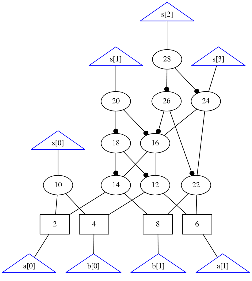
$\begin{array}[]{c@{\qquad}l@{\qquad}l}\mbox{Index}&\mbox{Gate Polynomial}&\mbox{Gate constraint}\\ g_{0}&s_{3}-\ell_{24}&s_{3}=\ell_{24}\\ g_{1}&s_{2}-\ell_{28}&s_{2}=\ell_{28}\\ g_{2}&\ell_{28}-\ell_{26}\ell_{24}+\ell_{26}+\ell_{24}-1&\ell_{28}=\neg\ell_{26}\land\neg\ell_{24}\\ g_{3}&\ell_{26}-\ell_{22}\ell_{16}+\ell_{22}+\ell_{16}-1&\ell_{26}=\neg\ell_{22}\land\neg\ell_{16}\\ g_{4}&\ell_{24}-\ell_{22}\ell_{16}&\ell_{24}=\ell_{22}\land\ell_{16}\\ g_{5}&\ell_{22}-b_{1}a_{1}&\ell_{22}=b_{1}\land a_{1}\\ g_{6}&s_{1}-\ell_{20}&s_{1}=\ell_{20}\\ g_{7}&\ell_{20}-\ell_{18}\ell_{16}+\ell_{18}+\ell_{16}-1&\ell_{20}=\neg\ell_{18}\land\neg\ell_{16}\\ g_{8}&\ell_{18}-\ell_{14}\ell_{12}+\ell_{14}+\ell_{12}-1&\ell_{18}=\neg\ell_{14}\land\neg\ell_{12}\\ g_{9}&\ell_{16}-\ell_{14}\ell_{12}&\ell_{16}=\ell_{14}\land\ell_{12}\\ g_{10}&\ell_{14}-b_{1}a_{0}&\ell_{14}=b_{1}\land a_{0}\\ g_{11}&\ell_{12}-b_{0}a_{1}&\ell_{12}=b_{0}\land a_{1}\\ g_{12}&s_{0}-\ell_{10}&s_{0}=\ell_{10}\\ g_{13}&\ell_{10}-b_{0}a_{0}&\ell_{10}=b_{0}\land a_{0}\\ \end{array}$

Boolean Input Polynomials: $a_{1}^{2}-a_{1},a_{0}^{2}-a_{0},b_{1}^{2}-b_{1},b_{0}^{2}-b_{0}$
Specification ${\mathcal{S}}$: $8s_{3}+4s_{2}+2s_{1}+s_{0}-4a_{1}b_{1}-2a_{1}b_{0}-2a_{0}b_{1}-a_{0}b_{0}$

Figure 1: AIG and polynomial encoding of a 2-bit multiplier in the ring $\mathbb{Q}[X]$.

Example 1

Figure 1 shows an AIG representing a 2-bit multiplier. We denote the primary inputs by $a_{0},a_{1},b_{0},b_{1}$ and outputs by $s_{0},s_{1},s_{2},s_{3}$. The internal nodes are denoted by $\ell_{i}$. The right hand side of Figure 1 lists the gate constraints as well as the corresponding gate polynomials. We furthermore list the Boolean input polynomials and the specification polynomial ${\mathcal{S}}\in\mathbb{Q}[X]$, which relates that $S=A\cdot B$, for $S=\sum_{i=0}^{3}2^{i}s_{i}$, $A=\sum_{i=0}^{1}2^{i}a_{i}$, and $B=\sum_{i=0}^{1}2^{i}b_{i}$.

3 Verification using Degree Reverse Lexicographic Order

In this section we will lay out the theoretical foundation of our proposed approach for extracting linear relations from the Gröbner basis that is used for reduction.

Existing algebraic verification techniques for acyclic graphs encode the circuit as a polynomial using a lexicographic term ordering where the variables are sorted according to a reverse topological term ordering (RTTO) [24]. This has the benefit that due to repeated application of Buchberger’s product criterion, see [8, Chap. 2, Sec. 10, Prop. 1], the set of gate polynomials together with the Boolean input polynomials automatically form a Gröbner basis [17]. Since the leading terms of the gate polynomials consist of one single variable, polynomial division comes down to substitution. The variables in the specification are substituted by the corresponding tails of the gate polynomials until no further rewriting is possible. The graph fulfills its specification if, and only if, the final result is zero. If the result is non-zero, the remainder polynomial consists of primary inputs only and can be used to derive a counter example.

Generally, this implies that the degree of the intermediate reduction results increases, since the tails of the gate polynomials have a higher degree than their linear leading terms. Substituting those variables in non-linear monomials has the potential to lead to a monomial blow-up during the reduction. A study in [25] showed that the intermediate reduction results for 16-bit multipliers can have more than $10^{6}$ monomials.

Example 2

Consider again the polynomials of Example 1. Initially $\operatorname{size}({\mathcal{S}})=8$ and $\deg({\mathcal{S}})=2$. After four rewriting steps we have the following intermediate reduction result: ${\mathcal{S}}\rightarrow_{\{g_{1},g_{2},g_{3},g_{4}\}}4\ell_{24}\ell_{22}\ell_{16}-4\ell_{24}\ell_{22}-4\ell_{24}\ell_{16}+8\ell_{24}-4\ell_{22}\ell_{16}+4\ell_{22}+2s_{1}+4\ell_{16}+s_{0}-4a_{1}b_{1}-2a_{1}b_{0}-2a_{0}b_{1}-a_{0}b_{0}$ which has degree 3 and consists of 13 monomials.

In this paper, we will now apply an orthogonal approach. We impose a different ordering on the set of gate polynomials that takes the degree of the polynomials into account. That is, we compute a Gröbner basis based on the degree reverse lexicographic monomial ordering, where the monomials in a polynomial are first sorted according to their degree.

Our approach is based on the following result that we prove in Theorem 3.1: If the specification polynomial is linear, then the ideal membership of the specification can be decided using only the linear polynomials of the Gröbner basis.

We linearize the specification by replacing all non-linear monomials $\sigma_{i}$ in ${\mathcal{S}}$ with new extension variables $t_{i}$. For each replacement we generate a new polynomial constraint $t_{i}-\sigma_{i}$ and add it to the set of gate polynomials. This idea is not novel and was, for instance, used in [22], where the variables $t_{i}$ are called tableau variables. The following lemma proves that if the non-linear specification ${\mathcal{S}}$ is contained in the ideal generated by the gate polynomials, then the linearized specification ${\mathcal{S}}_{\operatorname{lin}}$ is contained in the ideal generated by the gate polynomials and extension polynomials.

Lemma 3

Let $p\in\mathbb{K}[X]$, $I\subseteq\mathbb{K}[X]$. Let $\Sigma=\{t_{i}-\sigma_{i}\mid t_{i}\notin X\land\sigma_{i}\in p\land\deg(\sigma_{i})>1\}$. Let $p_{\operatorname{lin}}$ be the polynomial where every non-linear monomial of $p$ is replaced by a corresponding extension variable $t_{i}$. Then we have $p\in I$ if and only if $p_{\operatorname{lin}}\in I+\langle\Sigma\rangle$.

Proof

Let $p=\sum_{\sigma_{i}\in p}c_{i}\sigma_{i}$, where the $c_{i}$’s are in $\mathbb{K}$. By definition, we can write $p_{\operatorname{lin}}=\sum_{\sigma_{i}\in p}c_{i}t_{i}$. Thus, $p_{\operatorname{lin}}=\sum_{\sigma_{i}\in p}c_{i}(t_{i}-\sigma_{i})+\sum_{\sigma_{i}\in p}c_{i}\sigma_{i}$. By hypothesis, the first sum is in $\langle\Sigma\rangle$ and the second one, which is $p$, only depends in variables $X$. Therefore, if $p\in I$, then $p_{\operatorname{lin}}\in I+\langle\Sigma\rangle$. Conversely, if $p_{\operatorname{lin}}\in I+\langle\Sigma\rangle$, then $p\in(I+\langle\Sigma\rangle)\cap\mathbb{K}[X]=I$ by construction of $I+\langle\Sigma\rangle$.

The following theorem proves soundness and completeness of our observation. That is, if we want to show ideal membership of a linear polynomial, the Gröbner basis of the ideal contains a set of linear polynomials $G_{1}$ that suffice for the deriving the ideal membership, all non-linear polynomials of the Gröbner basis can be neglected. This will shift the computational difficulties from the reduction to the Gröbner basis generation.

Theorem 3.1

Let $p\in\mathbb{K}[X]$ with $\deg(p)=1$, $I\subseteq\mathbb{K}[X]$ be an ideal. Let $G$ be a Gröbner basis of $I$ with respect to $\mathrel{\prec_{\operatorname{drl}}}$ and let $G_{1}=\{g\in G\mid\deg(g)\leq 1\}$. We have $p\in I$ if and only if $p\rightarrow_{G_{1}}0$. In particular, $p=\alpha_{1}g_{1}+\cdots+\alpha_{m}g_{m}$ with $g_{i}\in G_{1}$, $\alpha_{i}\in\mathbb{K}$.

Proof

First, let us observe that if $G_{1}$ contains a non-zero constant polynomial, then $I=\mathbb{K}[X]$ and $p$ necessarily reduces to $0$ by $G_{1}$.

We now assume that $G_{1}$ only contains polynomials of degree $1$. For $g\in G_{1}$, we write $g=\operatorname{lt}(g)+\operatorname{tail}(g)$, with $\deg(\operatorname{lm}(g))=1$ and $\deg(\operatorname{tail}(g))\leq 1$. Since $\deg(\operatorname{lm}(p))=1$ the division algorithm for computing the reduction of $p$ by $G$, see [8, Chap. 2, Sec. 3], will only select polynomials in $G$ whose leading monomials also have degree $1$, i.e. those in $G_{1}$. The reduction step will replace $p$ by $p-cg=\operatorname{tail}(p)-c\operatorname{tail}(g)$, for $c\in\mathbb{K}$, which has degree less or equal to $1$.

Since $p\in I$ if, and only if, $p\rightarrow_{G}0$, we have $p\in I$ if, and only if, $p\rightarrow_{G_{1}}0$.

We focus our discussion on the use case of formally verifying an AIG. However, it is important to emphasize that the theory, and in particular the result of Theorem 3.1, is not restricted to AIGs and can be applied to general DAGs. The key property of the graph for deriving a total degree reverse lexicographic order is that it must be acyclic.

The conclusion of Theorem 3.1 moreover shows that we can significantly simplify the algorithm for checking the ideal membership of ${\mathcal{S}}$. Instead of repeated polynomial substitution, with potential non-linear intermediate reduction results, we pick $g_{i}\in G_{1}$, such that $\operatorname{lm}(g_{i})=\operatorname{lm}({\mathcal{S}})$, multiply $g_{i}$ by a constant $\alpha_{i}$ such that $\operatorname{lc}({\mathcal{S}})=-\alpha_{i}\operatorname{lc}(g_{i})$ and add those two polynomials. Hence, we have replaced polynomial division by linear polynomial operations.

Therefore, we can apply the following approach to verify that an AIG fulfills its specification, see Alg. 1. We first encode the graph as a set of polynomials $G_{\operatorname{init}}$ (line 1), and linearize the specification (line 2) as described in Lemma 3. The set $G_{\operatorname{ext}}$ contains the extension polynomials. In the next step we compute a Gröbner basis w.r.t. $\mathrel{\prec_{\operatorname{drl}}}$ (line 3) and extract the linear polynomials $G_{1}$ (line 4). We calculate the remainder of the specification modulo the linear elements of the Gröbner basis (lines 5-8) until no further reduction is possible and return whether the final result is zero. The correctness of Alg. 1 follows from Theorem 3.1.

Input : Circuit $C$ in AIG format, Specification polynomial ${\mathcal{S}}$

Output : Determine whether $C$ fulfills the specification

1 $G_{\operatorname{init}}\leftarrow\text{Gate-Polynomials}(C)\cup\text{Boolean-Input-Polynomials}(C)$;

2 ${\mathcal{S}}_{\operatorname{lin}},G_{\operatorname{ext}}\leftarrow$ Linearize(${\mathcal{S}}$);

3 $G_{\operatorname{drl}}\leftarrow$ Compute-$\mathrel{\prec_{\operatorname{drl}}}$-Gröbner-Basis($G_{\operatorname{init}}\cup G_{\operatorname{ext}}$);

4 $G_{1}\leftarrow\{g\mid g\in G_{\operatorname{drl}}\land\deg(g)\leq 1\}$;

5 while $\operatorname{lm}({\mathcal{S}}_{\operatorname{lin}})\in\{\operatorname{lm}(g)|g\in G_{1}\}$ do

6       $p_{\operatorname{lin}}\leftarrow g\in G_{1}$ such that $\operatorname{lm}(g)=\operatorname{lm}({\mathcal{S}}_{\operatorname{lin}})$;

7       if $\nexists p_{\operatorname{lin}}$ then return $\bot$;

8       ${\mathcal{S}}_{\operatorname{lin}}\leftarrow$ Linear-Reduce(${\mathcal{S}}_{\operatorname{lin}},p_{\operatorname{lin}}$);

9      

10 end while

return ${\mathcal{S}}_{\operatorname{lin}}=0$

Algorithm 1 Linear Gröbner basis reduction

Example 3

Consider again the AIG of Example 1. First of all we define four extension variables $t_{ij}$ to encode the non-linear terms $a_{i}b_{j}$ for $i,j\in\{0,1\}$ and rewrite the specification to $8s_{3}+4s_{2}+2s_{1}+s_{0}-4t_{11}-2t_{10}-2t_{01}-t_{00}$. The four polynomial equations $t_{ij}-a_{i}b_{j}$ are added to the set of gate polynomials and we compute a Gröbner basis w.r.t. $\mathrel{\prec_{\operatorname{drl}}}$. The full Gröbner basis consisting of 52 polynomials is listed in Appendix 0.A.

Important for us are the first thirteen elements of the Gröbner basis, as those are the linear polynomials $G_{1}$:

$\begin{array}[]{l@{=\quad}l@{\qquad\qquad}l@{=\quad}l}g_{1}&\ell_{10}-t_{00}&g_{8}&\ell_{22}-t_{11}\\ g_{2}&s_{0}-\ell_{10}&g_{9}&\ell_{24}-\ell_{16}\\ g_{3}&\ell_{12}-t_{10}&g_{10}&\ell_{26}-\ell_{24}+\ell_{16}+t_{11}-1\\ g_{4}&\ell_{14}-t_{01}&g_{11}&\ell_{28}+2\ell_{24}-\ell_{16}-t_{11}\\ g_{5}&\ell_{18}-\ell_{16}+t_{01}+t_{10}-1&g_{12}&s_{2}-\ell_{28}\\ g_{6}&\ell_{20}+2\ell_{16}-t_{01}-t_{10}&g_{13}&s_{3}-\ell_{24}\\ g_{7}&s_{1}-\ell_{20}\\ \end{array}$

We derive that ${\mathcal{S}}\in\langle G_{1}\rangle$ as ${\mathcal{S}}=8g_{13}+4g_{12}+4g_{11}+2g_{7}+2g_{6}+g_{2}+g_{1}$.

In practice, however line 3 of Alg. 1 turns out to be a bottleneck, computing a single $\mathrel{\prec_{\operatorname{drl}}}$-Gröbner basis does not scale for larger AIGs.

We have also seen in Example 1 that 39 out of 52 polynomials in the computed Gröbner basis are non-linear. While these polynomials are needed to compute the full Gröbner basis of the ideal, they are not required for solving the ideal membership problem of the linear specification. Furthermore, from the 13 linear polynomials, only 7 are used to generate the specification. Hence, our generated Gröbner basis contains redundant and/or useless information. We will discuss a method to reduce the overhead by computing local Gröbner bases in the following section.

4 Locally extracting Linear Polynomials

The core idea of the optimized approach is to start from a $\mathrel{\prec_{\operatorname{lex}}}$-Gröbner basis and incrementally extract linear polynomials from a smaller set of gate polynomials instead of computing a single full $\mathrel{\prec_{\operatorname{drl}}}$-Gröbner basis for the whole input AIG. The algorithm is outlined in Alg. 2 and will be explained in more detail throughout the remainder of this section.

In a nutshell, we first encode the circuit using a lexicographic term ordering (line 1) and linearize the specification polynomial (line 2) with respect to the given circuit. After some preprocessing where we extract easily derivable linear polynomials (line 3), we rewrite the specification by generating linear polynomials on the fly (lines 4–9). We pick the gate polynomial $p$ that has the same leading term as the intermediate reduction result (line 5) and compute a $\mathrel{\prec_{\operatorname{drl}}}$-Gröbner basis for a sub-circuit of $C$ that includes $p$ (line 6) to receive the linearized polynomial $p_{\operatorname{lin}}$ that we use for reducing the specification (line 7). Let us now go into more detail of every step.

1

Input : Circuit $C$ in AIG format, Specification polynomial ${\mathcal{S}}$

Output : Determine whether $C$ fulfills the specification

2 $G_{\operatorname{init}}\leftarrow$ Row-Wise-RTTO-Polynomial-Encoding($C$);

3 ${\mathcal{S}}_{\operatorname{lin}},G_{\operatorname{ext}}\leftarrow$ Linearize-Spec-wrt-AIG(${\mathcal{S}},G_{\operatorname{init}}$);

$G\leftarrow$ Preprocessing($G_{\operatorname{ext}}$)       $\triangleright$See Section 4.1

4

5while $\operatorname{lm}({\mathcal{S}}_{\operatorname{lin}})\in\{\operatorname{lm}(g)|g\in G\}$ do

6       $p\leftarrow g\in G$ such that $\operatorname{lm}(g)=\operatorname{lm}({\mathcal{S}}_{\operatorname{lin}})$;

       $p_{\operatorname{lin}}\leftarrow$ Linearize-Single-Polynomial($p,G$)       $\triangleright$See Section 4.2

7       if $p_{\operatorname{lin}}$ = 0 then return $\bot$;

8       ${\mathcal{S}}_{\operatorname{lin}}\leftarrow$ Linear-Reduce(${\mathcal{S}}_{\operatorname{lin}},p_{\operatorname{lin}}$);

9      

10 end while

return ${\mathcal{S}}_{\operatorname{lin}}=0$

Algorithm 2 Verification-via-Locally-extracting-Linear-Polynomials

Encoding.

The AIG is encoded using gate polynomials and Boolean input polynomials as described in Def. 10 and 11 using a lexicographic term ordering. We choose a row-wise variable ordering that sorts variables based on their distance to the inputs. If nodes have an equal distance, we sort according to the value of the AIG node. For example, we would sort the variables in Example 1 as $a_{0}\mathrel{\prec_{\operatorname{lex}}}b_{0}\mathrel{\prec_{\operatorname{lex}}}a_{1}\mathrel{\prec_{\operatorname{lex}}}b_{1}\mathrel{\prec_{\operatorname{lex}}}\ell_{10}\mathrel{\prec_{\operatorname{lex}}}\ell_{12}\mathrel{\prec_{\operatorname{lex}}}\ell_{14}\mathrel{\prec_{\operatorname{lex}}}\ell_{22}\mathrel{\prec_{\operatorname{lex}}}s_{0}\mathrel{\prec_{\operatorname{lex}}}\ell_{16}\mathrel{\prec_{\operatorname{lex}}}\ell_{18}\mathrel{\prec_{\operatorname{lex}}}\ell_{20}\mathrel{\prec_{\operatorname{lex}}}\ell_{24}\mathrel{\prec_{\operatorname{lex}}}\ell_{26}\mathrel{\prec_{\operatorname{lex}}}\ell_{28}\mathrel{\prec_{\operatorname{lex}}}s_{1}\mathrel{\prec_{\operatorname{lex}}}s_{3}\mathrel{\prec_{\operatorname{lex}}}s_{2}$. In this order the output variable of a gate is always greater than its input variables, which automatically generates a $\mathrel{\prec_{\operatorname{lex}}}$-Gröbner basis.

Theorem 4 in [17] has shown that we can locally rewrite elements of the $\mathrel{\prec_{\operatorname{lex}}}$-Gröbner basis without jeopardizing the Gröbner basis property as long as the leading monomials remain the same. We apply the same technique and locally rewrite gate polynomials from quadratic to linear polynomials that will be used in the reduction.

Linearization of the Specification.

Lemma 3 provides us with a methodology on how to linearize the specification ${\mathcal{S}}$ by introducing extension variables to represent non-linear terms. However, some of the terms might already be contained in the polynomial encoding of the circuit. For those terms we can simply use the corresponding leading term in the specification. We first swipe through the set of gate polynomials and check whether the non-linear tail of a gate polynomial is contained in the specification. If this is the case, we replace the non-linear term by the corresponding leading term.

For instance, in Example 3 we have the gate polynomial $\ell_{22}-a_{1}b_{1}$. Hence, we do not require the extension variable $t_{11}$ to linearize ${\mathcal{S}}$. This equality $\ell_{22}=t_{11}$ is also contained as polynomial $g_{8}$ in the computed $\mathrel{\prec_{\operatorname{drl}}}$-Gröbner basis.

All non-linear terms of ${\mathcal{S}}$ that cannot be linearized using gate polynomials we introduce extension variables as described in Section 3.

At this point, our encoding consists of a linear specification polynomial and a set of quadratic gate polynomials and Boolean input polynomials that generate a Gröbner basis w.r.t. a lexicographic term ordering. The following subsections present how we linearize elements of the Gröbner basis.

4.1 Preprocessing

The goal of preprocessing is to eliminate variables and derive linear polynomials in the $\mathrel{\prec_{\operatorname{lex}}}$-Gröbner basis that can be identified using simple heuristics. We employ three steps of rewriting, depicted in Alg. 3.

1

Input : Set of poynomial encodings of gate constraints $G$

Output : Rewritten Set of Polynomial encodings $G$

2 $G\leftarrow$ Merge-Nodes-with-Equal-Inputs($G$);

3 $G\leftarrow$ Eliminate-Positive-Nodes($G$);

4 $G\leftarrow$ Propagating-Equivalent-Nodes($G$);

5 return $G$;

Algorithm 3 Preprocessing

Merge Nodes with Equal Inputs.

If multiple AIG nodes $\ell_{i},\ell_{j}$ have the same inputs $a,b$, we can express one gate polynomial using the other. For instance, in our running Example 1 the nodes $\ell_{24}=\ell_{22}\ell_{16}$ and $\ell_{26}=(1-\ell_{22})(1-\ell_{16})$ would be such a set of AIG nodes.

Every gate polynomial of an AIG node has degree two, and the quadratic term is the product of the input nodes. Hence, the non-linear term in those gate polynomials that have the same inputs is the same. We remove the non-linear term of the topologically larger polynomial by adding or subtracting the smaller polynomial. For instance, we derive $\ell_{26}-\ell_{24}+\ell_{22}+\ell_{16}-1$.

Furthermore, if at least one input $a,b$ has a different polarity in $\ell_{i}$ and $\ell_{j}$, we immediately can derive that the product $\ell_{i}\ell_{j}$ is equal to zero. Let $\ell_{i}-\bar{a}\bar{b}$, $\ell_{j}-\hat{a}\hat{b}$ be the corresponding gate polynomials, where $\bar{a}$ and $\hat{a}$ represent the polarity of $a$. We have $\ell_{i}\ell_{j}=\bar{a}\bar{b}\hat{a}\hat{b}=0$, since $(\bar{a}=1-\hat{a})\lor(\bar{b}=1-\hat{b})$ holds. Thus, we can always remove the term $\ell_{i}\ell_{j}$ in a possible parent node, for instance the monomial $\ell_{26}\ell_{24}$ in $\ell_{28}$ in Example 1 can be removed.

Eliminate Positive Nodes.

In this step we eliminate nodes which are only non-negated inputs to other nodes in the graph. This heuristic was already considered in [14]. Since we restrict this heuristic to positive inputs, we can simply replace every occurrence of the node by the corresponding tail in the gate polynomial of the parent node. This, will increase the degree of the parent polynomial. However, we can check whether parts of the new tail term of the parent are equal to the tail term of another gate polynomial. If yes, we can reduce the tail term and include the leading term. This will decrease the temporal increase of the polynomial degree and furthermore will impose a node sharing which will be useful in later Gröbner basis computations. For instance, consider the polynomials $f-da,e-ca,d-cb$. We can derive $f-cba=f-eb$.

Propagating Equivalent Nodes.

If at any point in the rewriting we derive a linear polynomial of the form $\ell_{i}-\ell_{j}$ or $\ell_{i}+\ell_{j}-1$ we know that $\ell_{i}$ is equal to either $\ell_{j}$ or to its negation $1-\ell_{j}$. We propagate this information by eliminating the topologically larger node $\ell_{i}$ from the polynomial encoding. We choose to eliminate $\ell_{i}$ and not $\ell_{j}$ in order to not mess up the reverse topological term ordering for parent nodes of $\ell_{j}$. Propagation of equivalent nodes may not directly lead to linear gate polynomials, but helps to reduce the overall number of variables.

4.2 Linear Reduction

After preprocessing we repeatedly rewrite the linearized specification by the polynomial $p$ in the Gröbner basis that has the same leading monomial as the specification (line 5 in Alg. 2). For doing so, we need to linearize $p$. The pseudo-code is listed in Alg. 4. By Theorem 3.1, we know that a $\mathrel{\prec_{\operatorname{drl}}}$-Gröbner basis of a circuit must contain a linear polynomial $p_{\operatorname{lin}}$ with the same leading monomial as $p$. If this condition is not met, then the circuit does not satisfy the specification, as we cannot further reduce ${\mathcal{S}}$.

1

Input : Polynomial $p$, Polynomial system $G$

Output : Linear polynomial $p_{\operatorname{lin}}$ or 0

2

3$v\leftarrow\operatorname{lm}(p);d\leftarrow 3$ ;

4 while $d\leq\operatorname{dist}(v)$ do

5       $C_{v}\leftarrow\{v\}\cup\{\text{Children-up-to-Distance}(v,d)\}\cup\{\text{Siblings}(v)\}$;

6      

7      $C_{v}\leftarrow C_{v}\cup\{\text{Parents}(C_{v})\}$;

8       $G_{v}\leftarrow\text{Gate-Polynomials}(C_{v},G)\cup\text{Boolean-Input-Polynomials}(C_{v})$;

9      

10      $G_{\operatorname{drl}}\leftarrow$ Compute-$\mathrel{\prec_{\operatorname{drl}}}$-Gröbner-Basis ($G_{v}$);

11       if $\exists p_{\operatorname{lin}}\in G_{\operatorname{drl}}$ such that $\deg(p_{\operatorname{lin}})=1\land\operatorname{lm}(p_{\operatorname{lin}})=v$ then return $p_{\operatorname{lin}}$;

12       $d\leftarrow d+1$;

13      

14 end while

15

16return 0;

17

Algorithm 4 Linearize-Single-Polynomial

Let $v=\operatorname{lm}(p)$. We aim to compute a Gröbner basis w.r.t. a $\mathrel{\prec_{\operatorname{drl}}}$-ordering for a sub-circuit $C_{v}$ of $C$. The sub-circuit $C_{v}$ is constructed by including $v$ and all children nodes of $v$ up to a maximum distance $d$. Initially, we set $d=2$. If, during this process, we encounter a child node that already has a linear polynomial representation, we do not further add its children. This allows us to avoid unnecessary computations by excluding parts of the circuit that have already been simplified. Additionally, we include all smaller sibling nodes of $v$. Siblings are nodes that share at least one child with $v$. Moreover, we collect all parent nodes whose children are already included in the current set of nodes. This ensures that all relevant dependencies in the sub-circuit are captured.

This set of nodes represents the part of the circuit on which we will compute a local $\mathrel{\prec_{\operatorname{drl}}}$-Gröbner basis. The goal is to make the Gröbner basis just big enough such that it contains a linear polynomial with leading term $v$.

If this local Gröbner basis does not contain the expected linear polynomial, it suggests that the sub-circuit $C_{v}$ is insufficient to capture the desired behavior. In such cases, we repeat the process with an increased distance $d$ of the sub-circuit by adding more nodes. This iterative process continues until either a linear polynomial is found, or, in the worst case we have computed a full $\mathrel{\prec_{\operatorname{drl}}}$-Gröbner basis for all gate polynomials that are topologically smaller than $v$.

While this approach guarantees the completeness of the verification process, it comes with a practical limitation: computational complexity. If the sub-circuit grows too large (i.e., if too many nodes need to be added to $C_{v}$), the computation of the $\mathrel{\prec_{\operatorname{drl}}}$-Gröbner basis becomes infeasible in practice.

5 Experimental Evaluation

We evaluate our proposed approach on a set of multiplier benchmarks for different input bit-widths $n$. For all the circuits we have ${\mathcal{S}}=\sum_{i=0}^{2n}2^{i}s_{i}-(\sum_{i=0}^{n}2^{i}a_{i})\cdot(\sum_{i=0}^{n}2^{i}b_{i})$, hence choose $\mathbb{K}=\mathbb{Q}$. Since all the leading coefficients of the gate polynomials are 1, the computation will actually stay in the ring $\mathbb{Z}[X]\subseteq\mathbb{Q}[X]$ [16].

5.1 Implementation

We implement Alg. 2 in our tool MultiLinG, written in C++. We employ the following features:

• MultiLinG uses the polynomial arithmetic module from AMulet2 [15], which is targeted towards polynomial arithmetic where the variables represent Boolean values and the coefficients are integer values. In particular, the arithmetic engine automatically includes reasoning over the Boolean input polynomials, by reducing exponents, i.e., it calculates $x\cdot x=x$ internally.

• We sort the variables based on their minimum distance to the primary inputs to sort all extension variables next to the primary inputs, which gave us better practical results than the column-wise variable order from AMulet2.

• As a consequence of the row-wise order, we do not apply an incremental column-wise reduction algorithm [17], but rewrite the complete specification.

• For computing the $\mathrel{\prec_{\operatorname{drl}}}$-Gröbner basis, we use the msolve [3] library. Since msolve is designed for general purposes, we have to explicitly provide the Boolean input polynomials.

• If the linearization of individual polynomials fails and the distance of the node to the primary inputs is below six, we switch to non-linear rewriting as a fall-back option.

• In contrast to AMulet2, we do not support proof logging at the moment, as have not yet annotated msolve with corresponding proof logging steps. This is part of future work.

In case of acceptance, we will prepare an artifact that will be submitted to the voluntary artifact evaluation of TACAS.

5.2 Setup

We run our experiments on a Intel i7-1260P CPU. The time is listed in rounded seconds (wall-clock time). The time limit for the aoki-benchmarks is $300\text{\,}\mathrm{s}$, for the ABC-benchmarks it is set to $1200\text{\,}\mathrm{s}$. We set the memory limit to $1000\text{\,}\mathrm{MB}$. We compare MultiLinG against the algebraic approaches of AMulet2 [15], TeluMA [14], and DynPhaseOrderOpt [18]. The tools of related works [23] and [21] are not publicly available.

Benchmarks.

We evaluate our approach on integer multiplier circuits. Multipliers consist of three main components: partial product generation (PPG), partial product accumulation (PPA), and a final-stage adder (FSA). Each component has optimized architectures to reduce space and delay.

Two encodings are frequently used for PPG: simple AND-gate-based generation or Booth encoding. In the former case, every partial product $a_{i}b_{j}$ is explicitly computed, hence we do not require extension variables in our approach. For Booth encoding, we require extension variables as the partial products are internally combined. During PPA, partial products are accumulated, with the final two layers summed in the FSA.

In structured circuits, PPG, PPA, and FSA are clearly defined, benefiting tools like AMulet2 and TeluMA that require a clear cut between PPA and FSA to simplify the FSA. In synthesized circuits, gates are merged and rewritten to optimize the circuit, which blurs these component boundaries, and complicates direct verification. We consider two sets of benchmarks:

• aoki-multipliers [13]: This set of benchmarks contains 192 different non-synthesized multiplier architectures with an input bit-width 64.

• synthesized ABC multipliers [1]: These multipliers are generated using different types of standard synthesis scripts within ABC: resyn, resyn2, resyn3, dc2. We include a complex script that combines several synthesis techniques.

5.3 Results

ABC-benchmarks			Related work			MultiLinG
$n$	Synthesis	Nodes	[14]	[15]	[18]	Time	MergedNodes	PosNodes	LocalGB
32	resyn	7840	0.1	TO	0.2	0.3	1948	1	10
32	resyn2	7840	0.1	TO	0.3	0.3	1948	1	9
32	resyn3	7840	0.1	0.1	0.3	0.2	1952	0	0
32	dc2	7840	0.1	0.1	0.2	0.3	1952	0	0
32	complex	7839	TO	TO	0.2	0.4	1948	0	9
64	resyn	32064	0.3	TO	1.0	5.6	7996	1	10
64	resyn2	32064	0.2	TO	1.0	5.9	7996	1	9
64	resyn3	32064	0.3	0.2	1.0	5.6	8000	0	0
64	dc2	32064	0.2	0.3	1.0	5.8	8000	0	0
64	complex	32063	TO	TO	1.0	6.3	7996	0	9
128	resyn	129664	1.3	TO	5.7	200.6	32380	1	10
128	resyn2	129664	1.2	TO	6.4	214.1	32380	1	9
128	resyn3	129664	1.2	TO	7.7	209.3	32384	0	0
128	dc2	129664	1.1	TO	6.6	214.6	32384	0	0
128	complex	129663	TO	TO	5.8	214.1	32380	0	9

Table 1: Results on ABC benchmarks with bit-width $n$.

Figure 2: Results of aoki-benchmarks

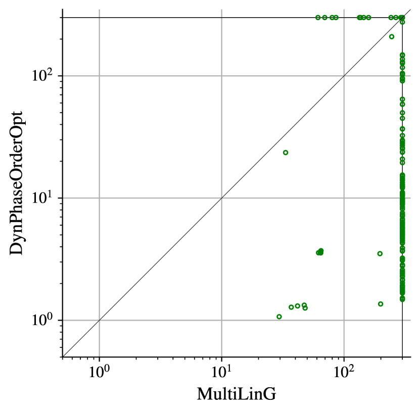
Figure 3: Comparing MultiLinG and DynPhaseOrderOpt

The results for the synthesized ABC multipliers are shown in Table 1. The heuristics of AMulet2 and TeluMA are not robust for these benchmarks and produce time outs. DynPhaseOrderOpt and our tool MultiLinG are both able to solve all benchmarks within the time limit of 300 seconds. We provide statistics on MultiLinG and show how often nodes with equal inputs are merged (“MergedNodes”), the number of eliminated positive nodes (“PosNodes”), and how often a local $\mathrel{\prec_{\operatorname{drl}}}$-Gröbner basis is computed (“LocalGB”). In none of the benchmarks we detected equivalent nodes. Interestingly for “resyn3” and “dc2” everything could be linearized via merging nodes with equal inputs.

Figure 3 shows the results on the aoki-benchmarks. Both, TeluMA and AMulet2, are able to solve the complete benchmark set. DynPhaseOrderOpt solves 163 out of 192 benchmarks, whereas our approach is only able to solve 30 benchmarks. Although the number of solved instances is low for MultiLinG, we are able to solve 14 out of the 29 benchmarks that DynPhaseOrderOpt does not cover, which is shown in Figure 3. As an example, among those 14 instances is a circuit consisting of a simple PPG, a grid-like PPA, and a carry-lookahead adder as FSA. The circuit has 53861 nodes and it was solved in MultiLinG by merging nodes with equal inputs 8002 times, removing positive nodes 7811 times and finally computing a local $\mathrel{\prec_{\operatorname{drl}}}$-Gröbner basis 3999 times. All instances that MultiLinG could not solve timed out during the Gröbner bases computations.

Summarizing the evaluation, AMulet2 and TeluMA are highly efficient on the structured circuits but are not robust on synthesized benchmarks. DynPhaseOrderOpt and MultiLinG are both robust and complement each other on complex multiplier designs. Hence we believe that our proposed approach is a valuable addition to the algebraic verification landscape and will be even more powerful when it is combined with existing methods.

6 Conclusion

In this paper we have presented a novel technique to verify directed acyclic graphs using computer algebra. Our first contribution is a theoretical theorem that shows how we can perform the ideal membership test of a specification polynomial using only linear polynomial operations. Secondly, we discuss how we can apply this theorem in practice to overcome the double-exponential complexity of computing a Gröbner basis. We present a technique that incrementally computes Gröbner bases for small sub-graphs to extract the linear information of the polynomials. We have demonstrated the potential of our approach on a set of multiplier circuits that have been challenging to verify so far.

In the future we aim to turn the black-box Gröbner basis approach into a white-box and explore how we can derive the linear polynomials without the computation of a full Gröbner basis. We also envision equivalence checking as a potential application, as this restricts the computation to Boolean polynomials.

6.0.1 Acknowledgements

This research was funded in part by the Austrian Science Fund (FWF) [ESPRIT 10.55776/ESP666], the joint ANR-FWF ANR-19-CE48-0015 ECARP and ANR-22-CE91-0007 EAGLES projects, the ANR-19-CE40-0018 De Rerum Natura project, and grants DIMRFSI 2021-02–C21/1131 of the Paris Île-de-France Region and FA8665-20-1-7029 of the EOARD-AFOSR.

Appendix 0.A Complete Gröbner basis for two-bit multiplier

⬇

gb[1]=l10-t00 gb[27]=l16*a1-l16

gb[2]=s0-l10 gb[28]=b0^2-b0

gb[3]=l12-t10 gb[29]=t10*b0-t10

gb[4]=l14-t01 gb[30]=t00*b0-t00

gb[5]=l18-l16+t01+t10-1 gb[31]=l16*b0-l16

gb[6]=l20+2*l16-t01-t10 gb[32]=b1^2-b1

gb[7]=s1-l20 gb[33]=t11*b1-t11

gb[8]=l22-t11 gb[34]=t10*b1-t11*b0

gb[9]=l24-l16 gb[35]=t01*b1-t01

gb[10]=l26-l24+l16+t11-1 gb[36]=t00*b1-t01*b0

gb[11]=l28+2*l24-l16-t11 gb[37]=l16*b1-l16

gb[12]=s2-l28 gb[38]=t11^2-t11

gb[13]=s3-l24 gb[39]=t10*t11-t11*b0

gb[14]=a0^2-a0 gb[40]=t01*t11-t11*a0

gb[15]=b0*a0-l10 gb[41]=t00*t11-l16

gb[16]=b1*a0-t01 gb[42]=l16*t11-l24

gb[17]=t01*a0-t01 gb[43]=t10^2-t10

gb[18]=t00*a0-t00 gb[44]=t01*t10-l16

gb[19]=l16*a0-l16 gb[45]=t00*t10-t10*a0

gb[20]=a1^2-a1 gb[46]=l16*t10-l16

gb[21]=b0*a1-t10 gb[47]=t01^2-t01

gb[22]=b1*a1-t11 gb[48]=t00*t01-t01*b0

gb[23]=t11*a1-t11 gb[49]=l16*t01+l16*t10+l20-t01-t10

gb[24]=t10*a1-t10 gb[50]=t00^2-t00

gb[25]=t01*a1-t11*a0 gb[51]=l16*t00-l16

gb[26]=t00*a1-t10*a0 gb[52]=l16^2-l16

References

- [1] Berkeley Logic Synthesis and Verification Group: ABC: A System for Sequential Synthesis and Verification. http://www.eecs.berkeley.edu/~alanmi/abc/ (2019), bitbucket Version 1.01
- [2] Berthomieu, J., Neiger, V., Safey El Din, M.: Faster Change of Order Algorithm for Gröbner Bases under Shape and Stability Assumptions. In: ISSAC. pp. 409–418. ACM (2022). https://doi.org/10.1145/3476446.3535484
- [3] Berthomieu, J., Eder, C., Safey El Din, M.: msolve: A Library for Solving Polynomial Systems. In: ISSAC. pp. 51–58. ACM (Jul 2021). https://doi.org/10.1145/3452143.3465545
- [4] Biere, A.: Collection of Combinational Arithmetic Miters Submitted to the SAT Competition 2016. In: SAT Competition 2016. Dep. of Computer Science Report Series B, vol. B-2016-1, pp. 65–66. University of Helsinki (2016)
- [5] Buchberger, B.: Ein Algorithmus zum Auffinden der Basiselemente des Restklassenringes nach einem nulldimensionalen Polynomideal. Ph.D. thesis, University of Innsbruck (1965)
- [6] Buchberger, B., Kauers, M.: Gröbner basis. Scholarpedia 5(10), 7763 (2010), http://www.scholarpedia.org/article/Groebner_basis
- [7] Chen, Y., Bryant, R.E.: Verification of Arithmetic Circuits with Binary Moment Diagrams. In: DAC. pp. 535–541. ACM (1995). https://doi.org/10.1145/217474.217583
- [8] Cox, D., Little, J., O’Shea, D.: Ideals, Varieties, and Algorithms. Springer-Verlag New York (1997)
- [9] Faugère, J.Ch.: A New Efficient Algorithm for Computing Gröbner bases (F4). Journal of Pure and Applied Algebra 139(1), 61–88 (1999). https://doi.org/10/bpq5dx
- [10] Faugère, J.Ch., Gaudry, P., Huot, L., Renault, G.: Sub-Cubic Change of Ordering for Gröbner Basis: A Probabilistic Approach. In: ISSAC. pp. 170–177. ACM (2014). https://doi.org/10.1145/2608628.2608669
- [11] Faugère, J.Ch., Gianni, P., Lazard, D., Mora, T.: Efficient Computation of Zero-dimensional Gröbner Bases by Change of Ordering. J. Symbolic Comput. 16(4), 329–344 (1993). https://doi.org/10/dv8t4j
- [12] Faugère, J.Ch., Mou, C.: Sparse FGLM algorithms. Journal of Symbolic Computation 80(3), 538–569 (2017). https://doi.org/10/gfz47c
- [13] Homma, N., Watanabe, Y., Aoki, T., Higuchi, T.: Formal Design of Arithmetic Circuits Based on Arithmetic Description Language. IEICE Trans. Fundam. Electron. Commun. Comput. Sci. 89-A(12), 3500–3509 (2006). https://doi.org/10.1093/IETFEC/E89-A.12.3500
- [14] Kaufmann, D., Beame, P., Biere, A., Nordström, J.: Adding dual variables to algebraic reasoning for gate-level multiplier verification. In: DATE. pp. 1431–1436. IEEE (2022). https://doi.org/10.23919/DATE54114.2022.9774587
- [15] Kaufmann, D., Biere, A.: Amulet 2.0 for verifying multiplier circuits. In: TACAS (2). LNCS, vol. 12652, pp. 357–364. Springer (2021). https://doi.org/10.1007/978-3-030-72013-1_19
- [16] Kaufmann, D., Biere, A., Kauers, M.: Verifying Large Multipliers by Combining SAT and Computer Algebra. In: FMCAD 2019. pp. 28–36. IEEE (2019). https://doi.org/10.23919/FMCAD.2019.8894250
- [17] Kaufmann, D., Biere, A., Kauers, M.: Incremental Column-wise verification of arithmetic circuits using computer algebra. Formal Methods Syst. Des. 56(1), 22–54 (2020). https://doi.org/10.1007/S10703-018-00329-2
- [18] Konrad, A., Scholl, C.: Symbolic Computer Algebra for Multipliers Revisited - It’s All About Orders and Phases. In: FMCAD 2024. TU Wien Academic Press (2024), to Appear.
- [19] Konrad, A., Scholl, C., Mahzoon, A., Große, D., Drechsler, R.: Divider verification using symbolic computer algebra and delayed don’t care optimization. In: FMCAD. pp. 1–10. IEEE (2022). https://doi.org/10.34727/2022/ISBN.978-3-85448-053-2_17
- [20] Kuehlmann, A., Paruthi, V., Krohm, F., Ganai, M.: Robust Boolean reasoning for equivalence checking and functional property verification. IEEE TCAD 21(12), 1377–1394 (2002). https://doi.org/10.1109/TCAD.2002.804386
- [21] Li, R., Li, L., Yu, H., Fujita, M., Jiang, W., Ha, Y.: Refscat: Formal verification of logic-optimized multipliers via automated reference multiplier generation and sca-sat synergy. IEEE TCAD pp. 1–1 (2024). https://doi.org/10.1109/TCAD.2024.3442987
- [22] Liew, V., Beame, P., Devriendt, J., Elffers, J., Nordström, J.: Verifying Properties of Bit-vector Multiplication Using Cutting Planes Reasoning. In: FMCAD 2020. FMCAD, vol. 1, pp. 194–204. TU Vienna Academic Press (2020). https://doi.org/10.34727/2020/ISBN.978-3-85448-042-6_27
- [23] Liu, H., Liao, P., Huang, J., Zhen, H.L., Yuan, M., Ho, T.Y., Yu, B.: Parallel gröbner basis rewriting and memory optimization for efficient multiplier verification. In: DATE. pp. 1–6 (2024). https://doi.org/10.23919/DATE58400.2024.10546568
- [24] Lv, J., Kalla, P., Enescu, F.: Efficient Gröbner Basis Reductions for Formal Verification of Galois Field Arithmetic Circuits. IEEE TCAD 32(9), 1409–1420 (2013). https://doi.org/10.1109/TCAD.2013.2259540
- [25] Mahzoon, A., Große, D., Drechsler, R.: PolyCleaner: Clean your Polynomials before Backward Rewriting to verify Million-gate Multipliers. In: ICCAD 2018. pp. 129:1 – 129:8. ACM (2018). https://doi.org/10.1145/3240765.3240837
- [26] Mahzoon, A., Große, D., Scholl, C., Drechsler, R.: Towards formal verification of optimized and industrial multipliers. In: DATE. pp. 544–549. IEEE (2020). https://doi.org/10.23919/DATE48585.2020.9116485
- [27] Neiger, V., Schost, É.: Computing syzygies in finite dimension using fast linear algebra. Journal of Complexity 60, 101502 (2020). https://doi.org/10.1016/j.jco.2020.101502
- [28] Sharangpani, H., Barton, M.L.: Statistical analysis of floating point flaw in the pentium processor (1994)
- [29] Temel, M.: Vescmul: Verified implementation of s-c-rewriting for multiplier verification. In: TACAS (1). LNCS, vol. 14570, pp. 340–349. Springer (2024). https://doi.org/10.1007/978-3-031-57246-3_19