Local Learning for Covariate Selection in Nonparametric Causal Effect Estimation with Latent Variables

Abstract

Estimating causal effects from nonexperimental data is a fundamental problem in many fields of science. A key component of this task is selecting an appropriate set of covariates for confounding adjustment to avoid bias. Most existing methods for covariate selection often assume the absence of latent variables and rely on learning the global network structure among variables. However, identifying the global structure can be unnecessary and inefficient, especially when our primary interest lies in estimating the effect of a treatment variable on an outcome variable. To address this limitation, we propose a novel local learning approach for covariate selection in nonparametric causal effect estimation, which accounts for the presence of latent variables. Our approach leverages testable independence and dependence relationships among observed variables to identify a valid adjustment set for a target causal relationship, ensuring both soundness and completeness under standard assumptions. We validate the effectiveness of our algorithm through extensive experiments on both synthetic and real-world data.

I Introduction

Estimating causal effects is crucial in various fields such as epidemiology [15], social sciences [39], economics [19], and artificial intelligence [31, 8]. In these domains, understanding and accurately estimating causal relationships are vital for policy making, clinical decisions, and scientific research. Within the framework of causal graphical models, covariate adjustment, such as the use of the back-door criterion [25], emerges as a powerful and primary tool for estimating causal effects from observational data, since implementing idealized experiments in practice is difficult [26]. Formally speaking, let $do(x)$ stand for an idealized experiment or intervention, where the values of $X$ are set to $x$, and $f(y|do(x))$ denote the causal effect of $X$ on $Y$. A valid covariate is a set of variables $\mathbf{Z}$ such that $f(y\mid do(x))=\int_{\mathbf{z}}f(y\mid x,\mathbf{z})f(\mathbf{z})d\mathbf{z}$ [26, 37]. Consider the graph (a) in Fig. 1, $\mathbf{Z}=\{V_{5}\}$ is a valid covariate set w.r.t. (with respect to) the causal relationship $X\to Y$.

Given a causal graph, one can determine whether a set is a valid adjustment set using adjustment criteria such as the back-door criterion [25, 26]. The main challenge in covariate adjustment estimation is to find a valid covariate set that satisfies the back-door criterion using only observational data, without the prior knowledge of the causal graph. To tackle this challenge, Maathuis et al. [22] proposed the IDA (Intervention do-calculus when the DAG (Directed Acyclic Graph) is Absent) algorithm. This algorithm first learns a CPDAG (Complete Partial Directed Acyclic Graph) using the PC (Peter-Clark) algorithm [38], enumerates all Markov equivalent DAGs, and estimates all possible causal effects of a treatment on an outcome. Additionally, with domain knowledge about specific causal directions, one can further identify more precise causal effects [30, 11]. For instance, Perkovic et al. [30] proposed the semi-local IDA algorithm, which provides a bound estimation of a causal effect when some directed edge orientation information is available. To efficiently find covariates, a local method CovSel utilizes criteria from [9] for covariate selection [13]. Though these methods have been used in a range of fields, they may fail to produce convincing results in cases with latent confounders, as they do not properly take into account the influences from latent variables [21].

There exists work in the literature that attempts to select covariates and estimate the causal effect in the presence of latent variables. Malinsky and Spirtes [24] introduced the LV-IDA (Latent Variable IDA) algorithm based on the generalized back-door criterion [21]. This algorithm initially learns a Partial Ancestral Graph (PAG) using the FCI (Fast Causal Inference) algorithm [39], then enumerates all Markov equivalent Maximal Ancestral Graphs (MAGs), and estimates all possible causal effects of a treatment on an outcome. Subsequently, Hyttinen et al. [18] proposed the CE-SAT (Causal Effect Estimation based on SATisfiability solver) method, which avoids enumerating all MAGs in the PAG. Although these algorithms are effective, learning the global causal graph is often unnecessary and wasteful when we are only interested in estimating the causal effects of specific relationships.

Figure 1: Example MAGs with treatment $X$ and outcome $Y$. Nodes shaded in blue represent a valid adjustment set. (a) Both global search EHS and local search CEELS methods identify the adjustment set. (b) Adapted from [5], CEELS fails to select the adjustment set despite the presence of a COSO variable $V_{1}$ (See Fig. 4 in Cheng et al. [5]). (c) An example without a COSO variable, where the adjustment set can still be found locally.

Several contributions have been developed to select covariates for estimating causal effects of interest without learning global causal structure. For instance, Entner et al. [10] designed two inference rules and proposed the EHS algorithm (named after the authors’ names) to determine whether a treatment has a causal effect on an outcome. If a causal effect is present, these rules help identify an appropriate adjustment set for estimating the causal effect of interest, based on the conditional independencies and dependencies among the observed variables. The EHS method has been demonstrated to be both sound and complete for this task. However, it is computationally inefficient, with time complexity of $\mathcal{O}(t\times 2^{t})$, where $t$ is the number of the observed covariates. It requires an exhaustive search over all combinations of variables for the inference rules. More recently, by leveraging a special variable, the Cause Or Spouse of the treatment Only (COSO) variable, combined with a pattern mining strategy [1], Cheng et al. [5] proposed a local algorithm, called CEELS (Causal Effect Estimation by Local Search), to select the adjustment set. Although the CEELS method is faster than the EHS method, it may fail to identify an adjustment set during the local search that could be found using a global search. For instance, considering the causal graphs (b) and (c) illustrated in Fig. 1, where $\{V_{2},V_{3},V_{4}\}$ and $\{V_{2},V_{3}\}$ are the valid adjustment sets w.r.t. $(X,Y)$ respectively. The CEELS algorithm fails to select these corresponding adjustment sets w.r.t. $(X,Y)$ , while the EHS method is capable of identifying them.

Contributions. It is desirable to develop a sound and complete local method to select an adjustment set for a causal relationship of interest. Specially, we make the following contributions:

• We propose a novel, fully local algorithm for selecting covariates in nonparametric causal effect estimation, utilizing testable independence and dependence relationships among the observed variables, and allowing for the presence of latent variables.

• We theoretically demonstrate that the proposed algorithm is sound and complete, and can identify a valid adjustment set for a target causal relationship (if such a set exists) under standard assumptions, comparable to global methods.

• We demonstrate the efficacy of our algorithm through experiments on both synthetic and real-world datasets.

II Related Work

This paper focuses on covariate selection in causal effect estimation within causal graphical models [26, 39]. Broadly speaking, the literature on covariate selection can be categorized into two main lines of research: methods that assume a known causal graph and methods that do not assume the availability of a causal graph. Below, we here provide a brief review of these two lines. For a comprehensive review of data-driven causal effect estimation, see [26, 29, 7].

Methods with Known Causal Graph. Ideally, when a causal graph is available, one can directly select an adjustment set for a causal relationship using the (generalized) back-door criterion [26, 21] or the (generalized) adjustment criterion [37, 29]. Research in this area often focuses on identifying special adjustment sets, such as minimal adjustment sets or ’optimal’ valid adjustment sets that have the smallest asymptotic variance compared to other adjustment sets. For selecting minimal adjustment sets, see [9, 40]. For ’optimal’ valid adjustment sets, one may refer to [14] for semi-parametric estimators or [34, 45, 36] for non-parametric estimators. In contrast to the aforementioned methods, this paper focuses on the identification of valid adjustment sets under unknown causal graphs.

Methods without Known Causal Graph. A classical framework for inferring causal effect is IDA (Intervention do-calculus when the DAG is Absent) [22]. IDA first learns a CPDAG and enumerates all Markov equivalent DAGs in the learned CPDAGs, then estimates all causal effects using the back-door criterion. Other notable developments along this line include combining prior knowledge [30, 11] or employing strategies through local learning [9]. However, these methods often assume causal sufficiency, meaning no latent confounders exist in the system, and thus do not adequately account for the influences of latent variables. To address this limation, a version of IDA suitable for systems with latent variables, known as LV-IDA (Latent Variable IDA), was proposed [24], based on the generalized back-door criterion [21]. Subsequently, more efficient methods were proposed by Hyttinen et al. [18], Wang et al. [44], and Cheng et al. [6]. Although these algorithms are effective, learning the global causal graph and estimating the causal effects for the entire system can be unnecessary and inefficient when the interest is solely on the causal effects of a single variable on an outcome variable. To address this issue, Entner et al. [10] proposed the EHS algorithm under the pretreatment assumption, demonstrating that the EHS method is both sound and complete for this task. However, the EHS approach is highly inefficient as it involves an exhaustive search over all possible combinations of variables for the inference rules. To overcome this inefficiency, Cheng et al. [5] introduced a local algorithm called CEELS for selecting the adjustment set. While CEELS is faster than the EHS proposed by [10], it may miss some adjustment sets during the local search that could be identified through a global search. In this paper, our work focuses on the same setting as EHS and introduces a fully local method for selecting the adjustment set. Compared to CEELS, our local method is both sound and complete, similar to the global learning method such as the EHS algorithm [10].

III Preliminaries

III-A Definitions

Graphs. A graph $\mathcal{G}=(\mathbf{V},\mathbf{E})$ consists of a set of nodes $\mathbf{V}=\{V_{1},\ldots,V_{p}\}$ and a set of edges $\mathbf{E}$. A graph $\mathcal{G}$ is directed mixed if the edges in the graph are directed ($\rightarrow$), or bi-directed ($\leftrightarrow$). A graph is a Directed Acyclic Graph (DAG) if it contains only directed edges and has no directed cycles. Given a graph $\mathcal{G}$, two nodes are said to be adjacent in $\mathcal{G}$ if there is an edge (of any kind) between them. A path $\pi$ in $\mathcal{G}$ is a sequence of distinct nodes $\left\langle V_{0},\ldots,V_{s}\right\rangle$ such that for $0\leq i\leq s-1$, $V_{i}$ and $V_{i+1}$ are adjacent in $\mathcal{G}$. A causal path (directed path) from $V_{i}$ to $V_{j}$ is a path composed of directed edges pointing towards $V_{j}$, i.e. , $V_{i}\rightarrow\ldots\rightarrow V_{j}$. A possibly causal path (possibly directed path) from $V_{i}$ to $V_{j}$ is a path where every edge without an arrowhead at the mark near $V_{i}$. A path from $V_{i}$ to $V_{j}$ that is not possibly causal is called a non-causal path from $V_{i}$ to $V_{j}$, e.g. , $V_{i}\leftarrow V_{i+1}\leftarrow\ldots\rightarrow V_{j-1}\rightarrow V_{j}$. A path $\pi$ from $V_{i}$ to $V_{j}$ is a collider path if $V_{i}$ and $V_{j}$ are adjacent or all the passing nodes are colliders on $\pi$, e.g. , $V_{i}\rightarrow V_{i+1}\leftrightarrow\ldots\leftrightarrow V_{j-1}\leftarrow V_{j}$. A node $V_{i}$ is a parent, child, or spouse of a node $V_{j}$ if there is $V_{i}\rightarrow V_{j}$, $V_{i}\leftarrow V_{j}$, or $V_{i}\leftrightarrow V_{j}$. $V_{i}$ is called an ancestor, or possible ancestor of $V_{j}$ and $V_{j}$ is a descendant, or possible descendant of $V_{i}$ if there is a causal path, or possibly causal path from $V_{i}$ to $V_{j}$ or $V_{i}=V_{j}$. A path $\pi$ between $V_{i}$ and $V_{j}$ is an inducing path if every non-endpoint vertex on $\pi$ is a collider and meanwhile an ancestor of either $V_{i}$ or $V_{j}$.

Definition 1 (m-separation).

In a directed mixed graph $\mathcal{G}$, a path $\pi$ between nodes $X$ and $Y$ is active (m-connecting) relative to a (possibly empty) set of nodes $\mathbf{Z}$ ($X,Y\notin\mathbf{Z}$) if 1) every non-collider on $\pi$ is not a member of $\mathbf{Z}$, and 2) every collider on $\pi$ has a descendant in $\mathbf{Z}$.

A set $\mathbf{Z}$ m-separates $\mathbf{X}$ and $\mathbf{Y}$ in $\mathcal{G}$, denoted by $(\mathbf{X}\mathrel{\perp\mspace{-10.0mu}\perp}\mathbf{Y}|\mathbf{Z})_{\mathcal{G}}$, if there is no active path between any nodes in $\mathbf{X}$ and any nodes in $\mathbf{Y}$ given $\mathbf{Z}$. The criterion of m-separation is a generalization of Pearl’s d-separation criterion in DAG to ancestral graphs.

Definition 2 (Ancestral Graph and Maximal Ancestral Graph (MAG)).

A directed mixed graph is called an ancestral graph if the graph does not contain any directed or almost directed cycles (ancestral) . In addition, an ancestral graph is a MAG if there is no inducing path between any two non-adjacent nodes (maximal) .

Ancestral graphs can be used to represent data-generating processes that may involve unobserved confounders, without explicitly modeling the unobserved variables [33]. Obviously, DAGs are special cases of ancestral graphs.

Definition 3 (Markov Equivalence).

Two MAGs $\mathcal{M}_{1}$, $\mathcal{M}_{2}$ are Markov equivalence if they share the same m-separations.

Basically a Partial Ancestral Graph represents an equivalence class of MAGs.

Definition 4 (Partial Ancestral Graph (PAG) [49]).

A Partial Ancestral Graph ($\mathit{PAG}$, denoted by $\mathcal{P}$) represents a $[\mathcal{M}]$, where a tail ‘$\--$’ or arrowhead ‘$>$’ occurs if the corresponding mark is tail or arrowhead in all the Markov equivalent MAGs, and a circle ‘$\circ$’ occurs otherwise.

In other words, PAG contains all invariant arrowheads and tails in all the Markov equivalent MAGs. For convenience, we use an asterisk (*) to denote any possible mark of a PAG ($\circ,>,\--$) or a MAG ($>,\--$).

Definition 5 (Visible Edges [48]).

Given a MAG $\mathcal{M}$ / PAG $\mathcal{P}$, a directed edge $X\rightarrow Y$ in $\mathcal{M}$ / $\mathcal{P}$ is visible if there is a node $S$ not adjacent to $Y$, such that there is an edge between $S$ and $X$ that is into $X$, or there is a collider path between $S$ and $X$ that is into $X$ and every non-endpoint node on the path is a parent of $Y$. Otherwise, $X\rightarrow Y$ is said to be invisible.

A visible edge $X\rightarrow Y$ means that there are no latent confounders between $X$ and $Y$.

Figure 2: Two configurations where the edge $X\rightarrow Y$ is visible. Nodes $S$ and $Y$ must be nonadjacent in (a) and (b).

Definition 6 ($\mathcal{G}_{\underline{X}}$ [21]).

For a MAG $\mathcal{M}$, let $\mathcal{M}_{\underline{X}}$ denote the graph obtained from $\mathcal{M}$ by removing all visible directed edges out of $X$ in $\mathcal{M}$. For a PAG $\mathcal{P}$, let $\mathcal{M}$ be any MAG consistent with $\mathcal{P}$ that has the same number of edges into $X$ as $\mathcal{P}$, and let $\mathcal{P}_{\underline{X}}$ denote the graph obtained from $\mathcal{M}$ by removing all directed edges out of $X$ that are visible in $\mathcal{M}$.

Definition 7 (Markov Blanket (MB)).

The Markov blanket of a variable $Y$, denoted as $\mathit{MB}(Y)$, is the smallest set conditioned on which all other variables are probabilistically independent of $Y$ , formally, $\forall V\in\mathbf{V}\setminus\{\mathit{MB(Y)}\cup V\}:Y\mathrel{\perp\mspace{-10.0mu}\perp}V\mid\mathit{MB(Y)}$.

Graphically, in a DAG, the Markov blanket of a node $Y$ includes the set of parents, children, and the parents of the children of $Y$. The Markov blanket of one node in a MAG is then defined as shown in Definition 8.

Definition 8 (MAG Markov Blanket [32, 27, 50]).

In a MAG $\mathcal{M}$, the Markov blanket of a node $Y$, noted as $\mathit{MMB(Y)}$, comprises 1) the set of parents, children, and children’s parents of $\ Y$; 2) the district of $\ Y$ and of the children of $\ Y$; and 3) the parents of each node of these districts. Where the district of a node $V$ is the set of all nodes reachable from $V$ using only bidirected edges.

Fig. 3 specifically illustrates the MAG Markov blanket of the node $Y$ in the MAG. The nodes shaded in blue belong to $\mathit{MMB(Y)}$.

Figure 3: The illustrative example for MMB in a MAG, where $\mathbf{Y}$ is the target of interest and the blue nodes belong to $\mathit{MMB(Y)}$.

Standard Assumption. The causal Markov condition says the m-separation relations among the nodes in a graph $\mathcal{G}$ imply conditional independence in probability relations among the variables. The causal Faithfulness condition states that m-connection in a graph $\mathcal{G}$ implies conditional dependence in the probability distribution [48]. Under the above two conditions, conditional independence relations among the observed variables correspond exactly to m-separation in the MAG or PAG $\mathcal{G}$, i.e., $(\mathbf{X}\mathrel{\perp\mspace{-10.0mu}\perp}\mathbf{Y}|\mathbf{Z})_{P}\Leftrightarrow(\mathbf{X}\mathrel{\perp\mspace{-10.0mu}\perp}\mathbf{Y}|\mathbf{Z})_{\mathcal{G}}$.

III-B Notations

The main symbols used in this paper are summarized in Table III-B. Sets of variables (nodes) are represented in bold, and individual variables (nodes) and symbols for graphs are in italics.

Symbol	Description
$\mathit{\mathcal{A}_{MMB}(X,Y)}$	A valid adjustment set in $\mathit{MMB(Y)}\setminus\{X\}$ w.r.t. $(X,Y)$
$\mathcal{R}1$	The rules in Theorem 2
$\mathcal{R}2$	The rules in Theorem 3
$\mathbf{V}$	The set of all variables, i.e., $\mathbf{V}=(X,Y)\cup\mathbf{O}\cup\mathbf{U}$
$X$	The treatment or exposure variable
$Y$	The outcome or response variable
$\mathbf{O}$	The set of observed covariates
$\mathbf{U}$	The set of latent variables
$\mathcal{G}$	A mix graph
$\mathcal{M}$	A Maximal Ancestral Graph (MAG)
$\mathcal{P}$	A Partial Ancestral Graph (PAG)
$t$	The number of the observed covariates, i.e., $t=|\mathbf{O}|$
$n$	The number of the observed covariates plus the pair of nodes $(X,Y)$, i.e., $n=|(X,Y)\cup\mathbf{O}|$
$\mathit{Adj(V_{i})}$	The set of adjacent nodes of $V_{i}$
$\mathit{MMB(V_{i})}$	The Markov blanket of a node $V_{i}$ in a MAG
$\mathit{PossDe(V_{i})}$	The set of all possible descendants of $V_{i}$
$(\mathbf{X}\mathrel{\perp\mspace{-10.0mu}\perp}\mathbf{Y}|\mathbf{Z})_{\mathcal{G}}$	A set $\mathbf{Z}$ m-separates $\mathbf{X}$ and $\mathbf{Y}$ in $\mathcal{G}$
$(\mathbf{X}\mathrel{\perp\mspace{-10.0mu}\perp}\mathbf{Y}|\mathbf{Z})_{P}$	$\mathbf{X}$ is statistically independent of $\mathbf{Y}$ given $\mathbf{Z}$. Without ambiguity, we often abbreviate $(\mathbf{X}\mathrel{\perp\mspace{-10.0mu}\perp}\mathbf{Y}|\mathbf{Z})_{P}$ as $\mathbf{X}\mathrel{\perp\mspace{-10.0mu}\perp}\mathbf{Y}|\mathbf{Z}$.
$(\mathbf{X}\centernot{\mathrel{\perp\mspace{-10.0mu}\perp}}\mathbf{Y}|\mathbf{Z})_{P}$	$\mathbf{X}$ is not statistically independent of $\mathbf{Y}$ given $\mathbf{Z}$
$\mathcal{G}_{\underline{X}}$	The graph obtained from $\mathcal{G}$ by removing all visible directed edges out of $X$ in $\mathcal{G}$

TABLE I: The list of main symbols used in this paper

III-C Adjustment Set

The covariate adjustment method is often used to estimate causal effects from observational data [26]. Throughout, we focus on the causal effect of a single treatment variable $X$ on the single outcome variable $Y$. One may refer to [29, 21, 41] for the details about the effect of a set of treatment variables $\mathbf{X}$ on a set of outcome variables $\mathbf{Y}$. We next introduce a more general graphical language to describe the covariate adjustment criterion, namely the generalized adjustment criterion [29]. Before providing its definition, we first introduce two important concepts in the graph, as they will be used in the description of this definition.

Definition 9 (Amenability [41, 29]).

Let $(X,Y)$ be a pair of nodes in a DAG, CPDAG, MAG, or PAG $\mathcal{G}$. The graph $\mathcal{G}$ is said to be adjustment amenable w.r.t. $(X,Y)$ if all proper possibly causal paths from $X$ to $Y$ start with a visible directed edge out of $X$.

Definition 10 (Forbidden set; $\mathit{Forb(X,Y)}$, [29]).

Let $(X,Y)$ be a pair of nodes in a DAG, CPDAG, MAG, or PAG $\mathcal{G}$. Then the forbidden set relative to $(X,Y)$ is defined as $\mathit{Forb(X,Y)}=\{W^{{}^{\prime}}\in\mathbf{V}\mid W^{{}^{\prime}}\in\mathit{PossDe(W)}$, $W$ lies on a proper possibly causal path from $X$ to $Y$ in $\mathcal{G}\}$.

Definition 11 (Generalized adjustment criterion [29]).

Let $(X,Y)$ be a pair of nodes in a DAG, CPDAG, MAG, or PAG $\mathcal{G}$. If a set of nodes $\mathbf{Z}\subseteq\mathbf{V}\setminus\{X,Y\}$ satisfies the generalized adjustment criterion relative to $(X,Y)$ in $\mathcal{G}$, i.e.,

• $\mathcal{G}$ is adjustment amenable relative to $(X,Y)$ , and

• $\mathbf{Z}\cap\mathit{Forb(X,Y)}=\emptyset$, and

• all proper definite status non-causal paths from $X$ to $Y$ are blocked by $\mathbf{Z}$ in $\mathcal{G}$.

then the causal effect of $X$ on $Y$ is identifiable and is given by

$$f(y\mid do(x))=\begin{cases}f(y\mid x)&if\;\mathbf{Z}=\emptyset,\\ \int_{\mathbf{z}}f(y\mid x,\mathbf{z})f(\mathbf{z})d\mathbf{z}&otherwise.\end{cases}$$ (1)

Note that the generalized adjustment criterion is equivalent to the generalized back-door criterion of Maathuis and Colombo [21] when the treatment $\mathbf{X}$ is a singleton. Thus, condition 3 can be represented by the requirement that all definite status back-door paths from $X$ to $Y$ are blocked by $\mathbf{Z}$ in $\mathcal{G}$.

Example 1 (Generalized adjustment criterion).

Consider the causal diagram shown in Fig. 4 (b). According to Definition 10, the MAG satisfies the amenability condition relative to $(X,Y)$ , and $\mathit{Forb(X,Y)}=\{Y\}$ holds true in the graph. Then, the set $\{V_{1},V_{2}\}$ is a valid adjustment set since, they can all block non-causal paths from $X$ to $Y$.

Figure 4: (a) An underlying causal DAG, adapted from Häggström [12], where $U_{1}$, and $U_{2}$ are unobserved variables. (b) The corresponding MAG of the DAG in (a).

III-D Problem Definition

We consider a Structural Causal Model (SCM) as described by Pearl [26]. The set of variables is denoted as $\mathbf{V}=(X,Y)\cup\mathbf{O}\cup\mathbf{U}$, with a joint distribution $P(\mathbf{V})$. Here, $\mathbf{O}$ represents the set of observed covariates, and $\mathbf{U}$ denotes the set of latent covariates. We assume there is no selection bias in the system. Therefore, the SCM is associated with a Directed Acyclic Graph (DAG), where each node corresponds to a variable in $\mathbf{V}$, and each edge represents a function $f$. Specifically, each variable $V_{i}\in\mathbf{V}$ is generated as $V_{i}=f_{i}(Pa(V_{i}),\varepsilon_{i})$, where $Pa(V_{i})$ denotes the parents of $V_{i}$ in the DAG, and $\varepsilon_{i}$ represents errors (or “disturbances”) due to omitted factors. In addition, all errors are assumed to be independent of each other. Analogous to Entner et al. [10], Cheng et al. [5], we assume that $Y$ is not a causal ancestor of $X$ , and that $\mathbf{O}$ is a set of pretreatment variables w.r.t. $(X,Y)$ , i.e. , $X$ and $Y$ are not causal ancestors of any variables in $\mathbf{O}$. It is noteworthy that existing methods commonly employ the pretreatment assumption [5, 10, 9, 42, 46]. This assumption is realistic as it reflects how samples are obtained in many application areas, such as economics and epidemiology [16, 19, 43]. For instance, every variable within the set $\mathbf{O}$ is measured prior to the implementation of the treatment and before the outcome is observed.

Task. Given an observational dataset $\mathcal{D}$ that consists of a pair of variables $(X,Y)$ , along with a set of covariates $\mathbf{O}$, we focus on a local learning approach to tackle the challenge of determining whether a specific variable $X$ has a causal effect on another variable $Y$, allowing for latent variables in the system. If such a causal effect is present, we aim to locally identify an appropriate adjustment set of covariates that can provide a consistent and unbiased estimator of this effect. Our method relies on analyzing the testable (conditional) independence and dependence relationships among the observed variables.

IV Local Search Adjustment Sets

In this section, we first present our theorems related to local search. Based on these theoretical results in Section IV-A, we then provide a local search algorithm to identify the valid adjustment set and show that it is both sound and complete in Section IV-B.

IV-A Local Search Theoretical Results

In this section, we provide the theoretical results for estimating the unbiased causal effect $X$ on $Y$ (if such an effect exists) solely from observational dataset $\mathcal{D}$. To this end, we need to locally identify the following three possible scenarios when the full causal structure is not known.

• $X$ has a causal effect on $Y$, and the causal effect is estimated by adjusting with a valid adjustment set.

• $X$ has no causal effect on $Y$.

• It is unknown whether there is a causal effect from $X$ on $Y$.

It should be emphasized that scenario $\mathcal{S}3$ arises because, under standard assumptions, based on the (testable) independence and dependence relationships among the observed variables, one may not identify a unique causal relationship between $X$ and $Y$. Typically, what we obtain is a Markov equivalence class encoding the same conditional independencies [39, 49, 10]. Thus, some of the causal relationships cannot be uniquely identified.

We now address scenario $\mathcal{S}1$. Before that, we define the adjustment set relative to $(X,Y)$ within the Markov blanket of $Y$ in a MAG (or PAG), denoted as $\mathit{\mathcal{A}_{MMB}(X,Y)}$. This definition will help us locally identify a valid adjustment set using testable independencies and dependencies, even in the presence of latent variables.

Definition 12 (Adjustment set in Markov blanket).

Let $X$ and $Y$ be a pair of treatment and outcome nodes in a MAG or PAG $\mathcal{G}$, where $\mathcal{G}$ is adjustment amenable w.r.t. $(X,Y)$ . A set $\mathbf{Z}$ is $\mathit{\mathcal{A}_{MMB}(X,Y)}$ if and only if (1) $\mathbf{Z}\subseteq\mathit{MMB(Y)}\setminus\{X\}$, (2) $\mathbf{Z}\cap\mathit{Forb(X,Y)}=\emptyset$, and (3) all non-causal paths from $X$ to $Y$ blocked by $\mathbf{Z}$.

The intuition behind the concept of $\mathit{\mathcal{A}_{MMB}(X,Y)}$ is as follows: In a graph without hidden variables, the causal effect of $X$ on $Y$ can be estimated using a subset of $\mathit{Pa(Y)}\setminus\{X\}$ [26]. However, in practice, some nodes in $\mathit{Pa(Y)}\setminus\{X\}$ may be unobserved. For instance, consider the MAG shown in Fig. 1 (b), where the edge $V_{4}\leftrightarrow Y$ indicates the presence of latent confounders. Consequently, the observed nodes do not include $\mathit{Pa(Y)}$. However, $\mathit{MMB(Y)}=\{X,V_{2},V_{3},V_{4}\}$ contains the valid adjustment set $\{V_{2},V_{3},V_{4}\}$. According to Definition 12, we know $\{V_{2},V_{3},V_{4}\}$ is an $\mathit{\mathcal{A}_{MMB}(X,Y)}$.

Remark 1.

Under our problem definition, since $\mathbf{O}$ is a set of pretreatment variables w.r.t. $(X,Y)$ , we have $\mathit{Forb(X,Y)}=\{Y\}$ and $Y$ not in $\mathit{MMB(Y)}$. Therefore, it is crucial to observe that the three conditions in Definition 12 can be simplified to two: (1) $\mathbf{Z}\subseteq\mathit{MMB(Y)}\setminus{X}$, and (2) all non-causal paths from $X$ to $Y$ are blocked by $\mathbf{Z}$.

One may raise the following question: if there does not exist a subset of $\mathit{MMB(Y)\setminus\{X\}}$ is an adjustment set w.r.t. $(X,Y)$ , then does an adjustment set w.r.t. $(X,Y)$ also not exist in the covariates $\mathbf{O}$? Interestingly, we find that the answer is yes, as formally stated in the following theorem.

Theorem 1 (Existence of $\mathit{\mathcal{A}_{MMB}(X,Y)}$).

Given an observational dataset $\mathcal{D}$ that consists of a pair of variables $(X,Y)$ , along with a set of covariates $\mathbf{O}$. There exists a subset of $\mathbf{O}$ is an adjustment set w.r.t. $(X,Y)$ if and only if there exists a subset of $\mathit{MMB(Y)\setminus\{X\}}$ is an adjustment set w.r.t. $(X,Y)$ , i.e. , $\mathit{\mathcal{A}_{MMB}(X,Y)}$.

Proof.

We begin by invoking Theorem 1 from Xie et al. [47], as it serves as a fundamental result necessary for proving Theorem 1.

Lemma 1.

[Theorem 1 of Xie et al. [47]] Let $Y$ be any node in $\mathbf{O}$, and $X$ be a node in $\mathit{MMB(Y)}$. Then $Y$ and $X$ are m-separated by a subset of $\mathbf{O}\setminus\left\{Y,X\right\}$ if and only if they are m-separated by a subset of $\mathit{MMB(Y)}\setminus\left\{X\right\}$.

The intuitive implications of Lemma 1 are as follows: Given a node $Y$ and another node $X$, where $X\in\mathit{MMB}(Y)$, if there is a subset of $\mathbf{O}\setminus\{Y,X\}$ that m-separates $Y$ and $X$, then there must exist a subset of $\mathit{MMB}(Y)\setminus\{X\}$ that m-separates $Y$ and $X$. Conversely, if no subset of $\mathit{MMB}(Y)\setminus\{X\}$ m-separates $Y$ and $X$, then no subset of $\mathbf{O}\setminus\{Y,X\}$ can m-separate $Y$ and $X$.

We now proceed to establish the proof of Theorem 1. According to Definition 11, a set $\mathbf{Z}$ is a valid adjustment set with respect to $(X,Y)$ in $\mathcal{P}$ if it satisfies all the conditions therein. When the treatment $X$ is a singleton, the generalized adjustment criterion becomes equivalent to the generalized back-door criterion proposed by Maathuis and Colombo [21]. Under our problem definition, the above conditions can be simplified: a set $\mathbf{Z}\subseteq\mathbf{O}$ is a valid adjustment set with respect to $(X,Y)$ if $\mathcal{P}$ is adjustment amenable relative to $(X,Y)$ (i.e., $X$ and $Y$ are connected by a visible edge, as a visible $X\rightarrow Y$) and $\mathbf{Z}$ m-separates $X$ and $Y$ in the $\mathcal{P}_{\underline{X}}$.

Equivalently, this is to show that a subset of $\mathbf{O}$ is an m-separating set with respect to $(X,Y)$ in $\mathcal{P}_{\underline{X}}$ if and only if a subset of $\mathit{MMB^{\prime}(Y)}$ is an m-separating set with respect to $(X,Y)$ in $\mathcal{P}_{\underline{X}}$, where $\mathit{MMB^{\prime}(Y)}$ denotes the MMB of $Y$ in $\mathcal{P}_{\underline{X}}$. Note that $\mathit{MMB^{\prime}(Y)}\subseteq\mathit{MMB}(Y)$, and $X$ may not belong to $\mathit{MMB^{\prime}(Y)}$ in $\mathcal{P}_{\underline{X}}$. We now analyze two cases:

Case 1: Suppose $\mathcal{P}$ is adjustment amenable relative to $(X,Y)$, with $X\in\mathit{MMB^{\prime}(Y)}$ in $\mathcal{P}_{\underline{X}}$, it follows that $X\notin\mathit{Adj(Y)}$. According to Lemma 1 and the fact that $X\in\mathit{MMB^{\prime}(Y)}$ in $\mathcal{P}_{\underline{X}}$, $X$ and $Y$ are m-separated by a subset of $\mathbf{O}$ if they are m-separated by a subset of $\mathit{MMB^{\prime}(Y)}\setminus\{X\}$ in $\mathcal{P}_{\underline{X}}$. If no subset of $\mathit{MMB^{\prime}(Y)}\setminus\{X\}$ m-separates $X$ and $Y$, then no subset of $\mathbf{O}\setminus\{X,Y\}$ can m-separate $X$ and $Y$, which implies $X\in\mathit{Adj(Y)}$ in $\mathcal{P}_{\underline{X}}$. This contradicts the assumption, thus proving that $\mathcal{P}$ is not adjustment amenable relative to $(X,Y)$ .

Case 2: Suppose $\mathcal{P}$ is adjustment amenable relative to $(X,Y)$, with $X\notin\mathit{MMB^{\prime}(Y)}$ in $\mathcal{P}_{\underline{X}}$, it follows that $X\notin\mathit{Adj(Y)}$. Thus, $X$ and $Y$ are m-separated by $\mathit{MMB^{\prime}(Y)}$, i.e. , $(X\mathrel{\perp\mspace{-10.0mu}\perp}Y\mid\mathit{MMB^{\prime}(Y)})_{\mathcal{P}_{\underline{X}}}$. If $(X\centernot{\mathrel{\perp\mspace{-10.0mu}\perp}}Y\mid\mathit{MMB^{\prime}(Y)})_{\mathcal{P}_{\underline{X}}}$, this contradicts the assumption, showing $\mathcal{P}$ is not adjustment amenable relative to $(X,Y)$ . Consequently, no subset of $\mathbf{O}\setminus\{X\}$ is a valid adjustment set with respect to $(X,Y)$ in $\mathcal{P}$.

∎

Theorem 1 states that if there exists a subset of $\mathbf{O}$ that is an adjustment set relative to $(X,Y)$ , then there exists a subset of $\mathit{MMB}(Y)\setminus\{X\}$ that is an adjustment set. Conversely, if no subset of $\mathit{MMB}(Y)\setminus\{X\}$ is an adjustment set, then no subset of $\mathbf{O}$ is an adjustment set relative to $(X,Y)$ .

Example 2.

Consider the MAG shown in Fig. 4 (b). We can identify $\mathit{MMB(Y)}$ from the MAG, i.e. , $\mathit{MMB(Y)}=\{X,V_{1},V_{2},V_{3},V_{4},V_{6}\}$. According to Definition 12 and the structure of the MAG, we can infer that any subset of $\mathit{MMB(Y)}\setminus\{X\}$ that includes $\{V_{1},V_{2}\}$ but excluding $\{V_{3}\}$ constitutes an $\mathit{\mathcal{A}_{MMB}(X,Y)}$.

Based on the Theorem 1, we next show that we can locally search for adjustment sets w.r.t. $(X,Y)$ in $\mathit{MMB(Y)}\setminus\{X\}$ by checking certain conditional independence and dependence relationships (Rule $\mathcal{R}1$), as stated in the following theorem. Meanwhile, we can locally find that $X$ has a causal effect on $Y$, i.e. , $\mathcal{S}1$.

Theorem 2 ($\mathcal{R}1$ for Locally Searching Adjustment Sets).

Given an observational dataset $\mathcal{D}$ that consists of a pair of variables $(X,Y)$ , along with a set of covariates $\mathbf{O}$. Then, a set $\mathbf{Z}\subseteq\mathit{MMB}(Y)\setminus\{X\}$ is $\mathit{\mathcal{A}_{MMB}(X,Y)}$ if

• $S\centernot{\mathrel{\perp\mspace{-10.0mu}\perp}}Y\mid\mathbf{Z}$, and

• $S\mathrel{\perp\mspace{-10.0mu}\perp}Y\mid\mathbf{Z}\cup\{X\}$

where $S\in\mathit{MMB}(X)\setminus\{Y\}$.

Proof.

Given $S\centernot{\mathrel{\perp\mspace{-10.0mu}\perp}}Y\mid\mathbf{Z}$, it follows that there exist active paths from $S$ to $Y$ conditional on $\mathbf{Z}$. Furthermore, $S\mathrel{\perp\mspace{-10.0mu}\perp}Y\mid\mathbf{Z}\cup{X}$ implies that all such active paths must necessarily pass through $X$, as the inclusion of $X$ in the conditioning set blocks all these paths.

Under the pretreatment assumption, $X$ is not a causal ancestor of any node in $\mathbf{O}$, and $X$ is excluded from the conditioning set for condition (i). Therefore, all active paths from $S$ to $Y$ given $\mathbf{Z}$ must include a directed edge from $X$ to $Y$. If $X$ were a collider, it would need to be included in the conditioning set for the paths to remain active. Consequently, these two conditions establish that $X$ exerts a causal effect on $Y$.

Suppose, for the sake of contradiction, that $\mathbf{Z}$ does not block all non-causal paths from $X$ to $Y$. Given $S\centernot{\mathrel{\perp\mspace{-10.0mu}\perp}}Y\mid\mathbf{Z}$ and $S\mathrel{\perp\mspace{-10.0mu}\perp}Y\mid\mathbf{Z}\cup\{X\}$, there must exist at least one active path from $S$ to $X$ conditional on $\mathbf{Z}$. This path, when combined with unblocked back-door paths from $X$ to $Y$, forms active paths from $S$ to $Y$ given $\mathbf{Z}\cup\{X\}$. However, this contradicts the condition $S\mathrel{\perp\mspace{-10.0mu}\perp}Y\mid\mathbf{Z}\cup\{X\}$. Thus, $\mathbf{Z}$ must block all non-causal paths from $X$ to $Y$, which establishes that $\mathbf{Z}$ satisfies the criteria of $\mathcal{A}_{MMB}(X,Y)$.

∎

Intuitively speaking, condition (i) indicates that there exist active paths from $S$ to $Y$ given $\mathbf{Z}$. Condition (ii) implies that there are no active paths from $S$ to $Y$ when given $\mathbf{Z}\cup\{X\}$. These two rules indicate that all active paths from $S$ to $Y$, given $\mathbf{Z}$, pass through $X$. Therefore, adding $X$ to the conditioning set blocks all active paths from $S$ to $Y$, given $\mathbf{Z}$. Hence, all non-causal paths from $X$ to $Y$ are blocked by $\mathbf{Z}$, otherwise, condition (ii) will not hold. Then, according to Definition 12, we know $\mathbf{Z}$ is an $\mathit{\mathcal{A}_{MMB}(X,Y)}$.

Example 3.

Consider the causal diagram depicted in Fig. 5 (b). Assume that an oracle performs conditional independence tests on the observational dataset $\mathcal{D}$. Consequently, we can determine the $\mathit{MMB(X)}$ and $\mathit{MMB(Y)}$, i.e. , $\mathit{MMB(X)}=\{V_{1},V_{2},V_{5},V_{6},V_{7},V_{8},V_{9},Y\}$, and $\mathit{MMB(Y)}=\{V_{1},V_{2},V_{5},V_{6},V_{8},V_{9},X\}$. According to Theorem 2, we can infer the existence of a causal effect of $X$ on $Y$. The set $\{V_{5},V_{6},V_{8}\}$ serves as an adjustment set $\mathit{\mathcal{A}_{MMB}(X,Y)}$, as $V_{7}\centernot{\mathrel{\perp\mspace{-10.0mu}\perp}}Y\mid\{V_{5},V_{6},V_{8}\}$ and $V_{7}\mathrel{\perp\mspace{-10.0mu}\perp}Y\mid\{V_{5},V_{6},V_{8},X\}$.

Figure 5: (a) An causal DAG, where $U_{i},i=1,...,4$ are latent variables. (b) The corresponding MAG of the DAG in (a).

Next, we provide the rule $\mathcal{R}2$ that allows us to locally identify $X$ has no causal effect on $Y$, i.e. , $\mathcal{S}2$.

Theorem 3 ($\mathcal{R}2$ for Locally Identifying No Causal effect).

Given an observational dataset $\mathcal{D}$ that consists of a pair of variables $(X,Y)$ , along with a set of covariates $\mathbf{O}$. Then, $X$ has no causal effect on $Y$ that can be inferred from the $\mathcal{D}$ if

• $X\mathrel{\perp\mspace{-10.0mu}\perp}Y\mid\mathbf{Z}$, or

• $S\centernot{\mathrel{\perp\mspace{-10.0mu}\perp}}X\mid\mathbf{Z}$, and $S\mathrel{\perp\mspace{-10.0mu}\perp}Y\mid\mathbf{Z}$

where $S\in\mathit{MMB}(X)\setminus\{Y\}$ and $\mathbf{Z}\subseteq\mathit{MMB}(Y)\setminus\{X\}$.

Proof.

Under the faithfulness assumption, condition (i) implies that there is no edge between $X$ and $Y$, and $X$ is not a causal ancestor of any nodes in $\mathbf{O}$. This implies that no causal path from $X$ to $Y$ exists unless there is a direct edge from $X$ to $Y$. Consequently, $X$ has no causal effect on $Y$.

Condition (ii) infers that $X$ and $Y$ are connected through a latent confounder. The condition $S\centernot{\mathrel{\perp\mspace{-10.0mu}\perp}}X\mid\mathbf{Z}$ ensures that there are active paths from $S$ to $X$ given $\mathbf{Z}$, and since $X$ is not a causal ancestor of any nodes in $\mathbf{O}$, these active paths must point to $X$. Furthermore, since $Y\notin\mathbf{Z}$ and $Y$ is neither a causal ancestor of any nodes in $\mathbf{O}$ nor of $X$, these active paths do not traverse $Y$. If there were a direct edge from $X$ to $Y$, it would create active paths from $S$ to $Y$, contradicting the condition $S\mathrel{\perp\mspace{-10.0mu}\perp}Y\mid\mathbf{Z}$. Therefore, there is no causal effect of $X$ on $Y$. ∎

According to the faithfulness assumption, condition (i) implies that $X$ and $Y$ are m-separated by a subset of $\mathit{MMB}(Y)\setminus\{X\}$. Thus, $X$ has a zero effect on $Y$. Condition (ii) provides a strategy to identify a zero effect even when a latent confounder exists between $X$ and $Y$. Roughly speaking, $S\centernot{\mathrel{\perp\mspace{-10.0mu}\perp}}X\mid\mathbf{Z}$ indicates that there are active paths from $S$ to $X$ given $\mathbf{Z}$. Therefore, if there were an edge from $X$ to $Y$, it would create an active path from $S$ to $Y$ by connecting to the previous path, which would contradict condition $S\mathrel{\perp\mspace{-10.0mu}\perp}Y\mid\mathbf{Z}$.

Example 4.

Consider the MAG shown in Fig. 4 (b). Assuming that the edge from $X$ to $Y$ is removed, then, we can infer that there is no causal effect of $X$ on $Y$ by condition (i), as $X\mathrel{\perp\mspace{-10.0mu}\perp}Y\mid\{V_{1},V_{2}\}$. Furthermore, suppose $V_{2}$ is a latent variable. Then, we can infer that there is no causal effect from $X$ to $Y$ by condition (ii), as $V_{6}\centernot{\mathrel{\perp\mspace{-10.0mu}\perp}}X\mid\{V_{1}\}$ and $V_{6}\mathrel{\perp\mspace{-10.0mu}\perp}Y\mid\{V_{1}\}$.

Lastly, we show that if neither $\mathcal{R}1$ of Theorem 2 nor $\mathcal{R}2$ of Theorem 3 applies, then one cannot identify whether there is a causal effect from $X$ on $Y$, based on conditional independence and dependence relationships among observational dataset $\mathcal{D}$, i.e. , we are in $\mathcal{S}3$.

Theorem 4.

Under the standard assumption, neither $\mathcal{R}1$ of Theorem 2 nor $\mathcal{R}2$ of Theorem 3 apply, then it is impossible to determine whether there is a causal effect from $X$ on $Y$, based on conditional independence and dependence relationships.

Proof.

Assuming Oracle tests for conditional independence tests. We first prove that $\mathcal{R}1$ in Theorem 2 is a necessary condition for identifying the existence of a causal effect of $X$ on $Y$ that based on the testable independencies and dependencies among the observed variables $\mathcal{D}$.

By the generalized adjustment criterion in Definition 11, there is a visible edge $X\rightarrow Y$ in $\mathcal{P}$. From the definition of a visible edge, such an edge $X\to Y$ is visible if and only if there exists a node $V$ (treated as $S$ in this proof) that is not adjacent to $Y$ and satisfies one of the following: (1) there is an edge between $V$ and $X$ that is into $X$, or (2) there is a collider path between $V$ and $X$ that is into $X$ and every non-endpoint node on the path is a parent of $Y$. Otherwise, $X\rightarrow Y$ is invisible.

Case 1: If there exists a node $S$ in $\mathcal{P}$ that satisfies the above case 1, and by Theorem 1, there is at least a set $\mathbf{Z}\subseteq\mathit{MMB(Y)\setminus\{X\}}$ block all non-causal paths from $X$ to $Y$. Thus, $S\centernot{\mathrel{\perp\mspace{-10.0mu}\perp}}X\mid\mathbf{Z}$ holds, adding $X$ to the condition set will block the path $S*\!\!\rightarrow X\rightarrow Y$, $S\centernot{\mathrel{\perp\mspace{-10.0mu}\perp}}Y\mid\mathbf{Z}\cup\{X\}$ holds.

Case 2: If there exists an $S$ in $\mathcal{P}$ that satisfies the above case 2, i.e. , there is a collider path between $S$ and $X$ that is into $X$ and every non-endpoint node on the path is a parent of $Y$, and $S$ not adjacent to $Y$. In this case, these collider nodes all belong to $\mathit{MMB(X)}$ and $\mathit{MMB(Y)}$. Assuming that there is no active path from $S$ to $X$, placing these collider nodes into the condition set will activate this $S$ to $X$ collider path. Thus, $S\centernot{\mathrel{\perp\mspace{-10.0mu}\perp}}X\mid\mathbf{Z}$ hold. In addition, these collider nodes must be in the condition set $\mathbf{Z}$ for block non-causal paths that pass these nodes. Thus, $\mathbf{Z}$ blocks all non-causal paths from $X$ to $Y$, but the newly activated path between $S$ and $X$ and the path after the $X\rightarrow Y$ merger are not blocked by $\mathbf{Z}$. Adding $X$ to the conditional set would then block this path, and thus $S\mathrel{\perp\mspace{-10.0mu}\perp}Y\mid\mathbf{Z}\cup\{X\}$ holds.

Consequently, these two cases prove that $\mathcal{R}1$ is a necessary condition for identifying the existence of a causal effect of $X$ on $Y$ based on the testable independencies and dependencies. Next, we prove that $\mathcal{R}2$ in Theorem 3 is a necessary condition for identifying the absence of a causal effect of $X$ on $Y$ using testable independence and dependence relationships among the observed variables. Under our problem definition, the causal structures discovered through testable conditional independence and dependencies between observable variables, that can infer $X$ has no causal effect on $Y$ can be divided into the following two cases: (1) there is no edge between $X$ and $Y$, (2) the edge between $X$ and $Y$ is $X\leftrightarrow Y$ in $\mathcal{P}$.

Case 1: If there is no edge between $X$ and $Y$, then by Lemma 1, if $X\in\mathit{MMB}(Y)$, there must exist a subset $\mathbf{Z}$ of $\mathit{MMB}(Y)\setminus\{X\}$ that m-separates $X$ and $Y$, i.e., $X\mathrel{\perp\mspace{-10.0mu}\perp}Y\mid\mathbf{Z}$, where $\mathbf{Z}\subseteq\mathit{MMB}(Y)\setminus\{X\}$. If $X\notin\mathit{MMB}(Y)$, then by Definition 7, $X\mathrel{\perp\mspace{-10.0mu}\perp}Y\mid\mathit{MMB}(Y)$.

Case 2: Since $Y$ and $X$ are not causal ancestors of any nodes in $\mathbf{O}$, and $Y$ is not a causal ancestor of $X$, then $X$ is a collider. If $X$ is an unshielded collider, then there exists a node $S$ in the $\mathcal{P}$ that is adjacent to $X$, but not $Y$. Such $S$ belong to $\mathit{MMB}(X)\setminus\{Y\}$ and $\mathit{MMB}(Y)\setminus\{X\}$. By Lemma 1, $S\mathrel{\perp\mspace{-10.0mu}\perp}Y\mid\mathbf{Z}$, where $\mathbf{Z}\subseteq\mathit{MMB(Y)}\setminus\{X\}$. In addition, $S\centernot{\mathrel{\perp\mspace{-10.0mu}\perp}}X\mid\mathbf{Z}$ due to $S$ is adjacent to $X$. If $X$ is a shielded collider, which can be inferred by testable conditional independence and dependencies between observable variables, then there exists a discriminating path $\pi$ for $X$ in the $\mathcal{P}$[49]. This path $\pi$ includes at least three edges, $X$ is a non-endpoint node on $\pi$ and is adjacent to $Y$ on $\pi$. The path has a node $S$ that is not adjacent to $Y$, and every node between $S$ and $X$ on $\pi$ is a collider and a parent of $Y$. These colliders between $S$ and $X$ belong to $\mathit{MMB}(X)$ and $\mathit{MMB}(Y)$, so including such nodes in the set $\mathbf{Z}$ implies $S\centernot{\mathrel{\perp\mspace{-10.0mu}\perp}}X\mid\mathbf{Z}$ and $S\mathrel{\perp\mspace{-10.0mu}\perp}Y\mid\mathbf{Z}$, where $\mathbf{Z}$ may contain some nodes belonging to $\mathit{MMB(Y)}$ in addition to those colliding nodes in order to m-separate $S$ and $Y$ (Lemma 1).

In summary, if neither $\mathcal{R}1$ nor $\mathcal{R}2$ applies, then we cannot infer whether there is a causal effect of $X$ on $Y$ from the independence and dependence relationships among the observed variables.

∎

Theorem 4 says that there may exist causal structures with and without an edge from $X$ to $Y$, which entail the same dependencies and independencies among the observational dataset $\mathcal{D}$. Consequently, it is not possible to uniquely infer whether there is a causal effect or not.

Example 5.

Consider the three graphs in Fig. 6. These graphs entail the same independencies and dependencies among the observed variables $(X,Y,V)$. Therefore, it is impossible to determine, based solely on testable dependencies and independence, whether $X$ has a causal effect on $Y$ and whether $V$ should be included in the adjustment set.

Figure 6: Three DAGs that entail the same independencies and dependencies among the observed variables $(X,Y,V)$, where $U_{1}$, $U_{2}$, and $U_{3}$ are latent variables.

IV-B The LSAS Algorithm

In this section, we leverage the above theoretical results and propose the Local Search Adjustment Sets ($LSAS$) algorithm to infer whether there is a causal effect of a variable $X$ on another variable $Y$, and if so, to estimate the unbiased causal effect. Given a pair of variables $(X,Y)$ , the algorithm consists of the following two key steps:

• Learning the MMBs of $X$ and $Y$: This involves using an MMB discovery algorithm to identify the Markov Blanket Members (MMBs) of both $X$ and $Y$.

• Determining Adjustment Sets: For each variable $S$ in $\mathit{MMB(X)}\setminus\{Y\}$, we check whether $S$ and the subsets $\mathbf{Z}$ of $\mathit{MMB(Y)}\setminus\{X\}$ satisfy rules $\mathcal{R}1$ and $\mathcal{R}2$ based on Theorems 2 $\sim$ 4.

The algorithm uses $\Theta$ to store the estimated causal effect of $X$ on $Y$. If $\Theta=0$, it indicates that there is no causal effect of $X$ on $Y$. If $\Theta$ is null, it suggests that the lack of knowledge to obtain the unbiased causal effect. Otherwise, $\Theta$ provides the estimated causal effect of $X$ on $Y$. The complete procedure is summarized in Algorithm 1, and the algorithm that we used for the MMB learning is in Algorithm 2.

Algorithm 1 $LSAS$

0:  Observed dataset $\mathcal{D}$, treatment $X$, outcome $Y$.

1:  $\mathit{MMB(X)},\mathit{MMB(Y)}\leftarrow\text{MMB learning}(X,Y,\mathcal{D})$

2:  $\Theta\leftarrow\emptyset$

3:  for each $V_{i}\in\mathit{MMB(X)}\setminus\{Y\}$ do

4:     $S\leftarrow V_{i}$

5:     for each set $\mathbf{Z}\subseteq\mathit{MMB(Y)}\setminus\{X\}$ do

6:        if $X\mathrel{\perp\mspace{-10.0mu}\perp}Y\mid\mathbf{Z}$ then

7:           $\Theta\leftarrow 0$

8:           Break

9:        else if $S\centernot{\mathrel{\perp\mspace{-10.0mu}\perp}}X\mid\mathbf{Z}$ then

10:           if $S\mathrel{\perp\mspace{-10.0mu}\perp}Y\mid\mathbf{Z}$ then

11:              $\Theta\leftarrow 0$

12:              Break

13:           else if $S\mathrel{\perp\mspace{-10.0mu}\perp}Y\mid\mathbf{Z}\cup\{X\}$ then

14:              Calculate the causal effect $\theta$ w.r.t. $(X,Y)$ given $\mathbf{Z}$

15:              Add $\theta$ to $\Theta$

16:           end if

17:        end if

18:     end for

19:  end for

19:  The causal effect $\Theta$.

The definition of the TC (Total Conditioning) [28] we used to discover MMBs is as follows:

Definition 13 (Total conditioning [28]).

In the context of a faithful causal graph $\mathcal{G}$, for any two distinct nodes $X,Y\in\mathbf{V}$, $X\in\mathit{MB(Y)}$ if and only if $X\centernot{\mathrel{\perp\mspace{-10.0mu}\perp}}Y\mid\mathbf{V}\setminus\{X,Y\}$.

Algorithm 2 MMB learning

0:  $X$, $Y$, observed covariates $\mathbf{O}$

1:  Initialize : $\mathit{MMB}(X)=\emptyset$, $\mathit{MMB}(Y)=\emptyset$.

2:  $CandSet=\mathbf{O}\cup\{X,Y\}$

3:  for each $V_{i}\in CandSet\setminus\{X\}$ do

4:     if $X\centernot{\mathrel{\perp\mspace{-10.0mu}\perp}}V_{i}\mid CandSet\setminus\{X,V_{i}\}$ then

5:        Add $V_{i}$ to $\mathit{MMB}(X)$

6:     end if

7:  end for

8:  for each $V_{i}\in CandSet\setminus\{X,Y\}$ do

9:     if $Y\centernot{\mathrel{\perp\mspace{-10.0mu}\perp}}V_{i}\mid CandSet\setminus\{Y,V_{i}\}$ then

10:        Add $V_{i}$ to $\mathit{MMB}(Y)$

11:     end if

12:  end for

12:  $\mathit{MMB(X)}$, $\mathit{MMB(Y)}$

We next demonstrate that in the large sample limit, the LSAS algorithm is both sound and complete.

Theorem 5 (The Soundness and Completeness of $LSAS$ Algorithm).

Assume Oracle tests for conditional independence tests. Under the assumptions stated in our problem definition (Section III-D), the LSAS algorithm correctly outputs the causal effect $\Theta$ whenever rule $\mathcal{R}1$ or $\mathcal{R}2$ applies. However, if neither rule $\mathcal{R}1$ nor $\mathcal{R}2$ applies, the LSAS algorithm can not determine whether there is a causal effect from $X$ on $Y$, based on the testable conditional independencies and dependencies among the observed variables.

Proof.

Assuming Oracle tests for conditional independence tests, the MMB discovery algorithm finds all and only the MMB nodes of a target variable.

Following Theorem 2 and Theorem 4, $\mathcal{R}1$ is a sufficient and necessary condition for identifying $X$ has a causal effect on $Y$ that can be inferred by testable (conditional) independence and dependence relationships among the observational variables, and there is a set $\mathbf{Z}$ is $\mathit{\mathcal{A}_{MMB}(X,Y)}$. Hence, if there is a causal effect of $X$ on $Y$ that can be inferred by observational data, then $LSAS$ can accurately identify the causal effect of $X$ on $Y$.

Subsequently, relying on Theorem 3 and Theorem 4, $\mathcal{R}2$ is a sufficient and necessary condition for identifying the absence of the causal effect of $X$ on $Y$ that can be inferred from observational data. Thus, $LSAS$ can correctly identify there is no causal effect of $X$ on $Y$ that can be inferred from observational data. Ultimately, if neither $\mathcal{R}1$ nor $\mathcal{R}2$ applies, then $LSAS$ cannot infer whether there is a causal effect of $X$ on $Y$ from the independence and dependence relationships between the observations.

Hence, the soundness and completeness of the $LSAS$ algorithm are proven. ∎

Formally, soundness means that, given an independence oracle and under the assumptions stated in our problem definition (Section III-D), the inferences made using rule $\mathcal{R}1$ or $\mathcal{R}2$ are always correct whenever these rules apply. On the other hand, completeness implies that if neither rule $\mathcal{R}1$ nor $\mathcal{R}2$ applies, it is impossible to determine, based solely on the conditional independencies and dependencies among the observed variables, whether $X$ has a causal effect on $Y$ or not.

Complexity of $LSAS$ Algorithm. The complexity of the $LSAS$ algorithm can be divided into two main components: the first component is the MMB discovery algorithm (Line 1), and the second involves locally identifying causal effects using $\mathcal{R}_{1}$ and $\mathcal{R}_{2}$ (Lines $3\sim 19$). Let $\mathit{n}$ represent the size of the set $\mathbf{O}$ plus the pair of nodes $(X,Y)$ . We utilized the TC (Total Conditioning) algorithm [28] to identify the MMB. Consequently, the time complexity of finding the MMB for two nodes is $\mathcal{O}(2n-3)$. In the worst-case scenario, the complexity of the second component is $\mathcal{O}[(|\mathit{MMB(X)}|-1)\times 2^{|\mathit{MMB(Y)}|-1}]$. Therefore, the overall worst-case time complexity of the $LSAS$ algorithm is $\mathcal{O}[(|\mathit{MMB(X)}|-1)\times 2^{|\mathit{MMB(Y)}|-1}+2n-3]$. Note that the complexity of the EHS algorithm is $\mathcal{O}[(n-2)\times 2^{n-2}]$, which is significantly higher than the complexity of our algorithm, particularly when $n\gg|\text{MMB}(Y)|$ in large causal networks. The CEELS algorithm [5] employs the PC.select algorithm [3] to search for $\mathit{Adj}(X)$ and $\mathit{Adj}(Y)$. In the worst-case scenario, the overall complexity of CEELS is $\mathcal{O}\left(n\times 2^{q}\right)$, where $q=\max(|\mathit{Adj}(X)\setminus{Y}|,|\mathit{Adj}(Y)\setminus{X}|)$. Although in practice, the complexity of CEELS may not differ significantly from that of our proposed algorithm, it is crucial to note that CEELS might miss an adjustment set during the local search that could otherwise be identified through a global search. This issue, as illustrated in Fig. 1(b), is not present in our proposed algorithm.

V Experimental Results

In this section, to demonstrate the accuracy and efficiency of our proposed method, we applied it to synthetic data with specific structures and benchmark networks, as well as to the real-world dataset . We here use the existing implementation of the Total Conditioning (TC) discovery algorithm [28] to find the MMB of a target variable. All experiments were conducted on Intel CPUs running at 2.90 GHz and 2.89 GHz, with 128 GB of memory.

TABLE II: Performance Comparisons on the Causal Graph in Fig. 4.

	Size=2K		Size=5K		Size=7K		Size=10K
Algorithm	RE($\%$)$\downarrow$	nTest$\downarrow$	RE($\%$)$\downarrow$	nTest$\downarrow$	RE($\%$)$\downarrow$	nTest$\downarrow$	RE($\%$)$\downarrow$	nTest$\downarrow$
PA	66.18 ± 155.54	-	45.68 ± 38.13	-	41.91 ± 27.13	-	43.34 ± 14.36	-
LV-IDA	69.00 ± 40.49	174.75 ± 45.12	60.80 ± 44.56	208.43 ± 52.79	44.10 ± 44.97	222.60 ± 51.18	32.64 ± 42.78	237.32 ± 56.68
EHS	33.72 ± 43.29	946.00 ± 0.00	28.64 ± 43.90	946.00 ± 0.00	26.90 ± 39.22	946.00 ± 0.00	12.66 ± 30.82	946.00 ± 0.00
CEELS	24.68 ± 35.16	174.85 ± 57.18	24.62 ± 36.97	196.96 ± 55.31	15.00 ± 28.83	210.00 ± 60.84	7.37 ± 18.79	224.76 ± 60.07
LSAS	23.63 ± 33.72	55.01 ± 19.56	15.39 ± 29.53	55.63 ± 19.24	10.47 ± 24.03	66.45 ± 20.37	3.49 ± 5.50	66.57 ± 20.25

• Note: $\downarrow$ means a lower value is better, and vice versa. The symbol ’-’ indicates that PA does not output this information.

TABLE III: Performance Comparisons on the Causal Graph in Fig. 5.

	Size=2K		Size=5K		Size=7K		Size=10K
Algorithm	RE($\%$)$\downarrow$	nTest$\downarrow$	RE($\%$)$\downarrow$	nTest$\downarrow$	RE($\%$)$\downarrow$	nTest$\downarrow$	RE($\%$)$\downarrow$	nTest$\downarrow$
PA	49.81 ± 12.02	-	44.15 ± 14.74	-	43.60 ± 14.33	-	41.42 ± 15.20	-
LV-IDA	44.23 ± 21.48	345.11 ± 105.03	35.09 ± 21.95	429.36 ± 112.00	24.29 ± 15.48	429.98 ± 114.88	20.39 ± 5.88	480.09 ± 98.28
EHS	28.48 ± 22.04	1656.00 ± 0.00	26.39 ± 17.47	1656.00 ± 0.00	21.07 ± 11.66	1656.00 ± 0.00	19.31 ± 15.21	1656.00 ± 0.00
CEELS	46.25 ± 34.77	391.20 ± 174.69	38.79 ± 25.91	455.94 ± 154.56	35.91 ± 26.69	464.46 ± 168.28	37.59 ± 32.93	537.22 ± 158.38
LSAS	27.40 ± 22.73	203.97 ± 19.22	24.06 ± 19.18	204.99 ± 6.67	18.93 ± 11.40	204.76 ± 6.19	14.46 ± 11.40	206.04 ± 5.14

• Note: $\downarrow$ means a lower value is better, and vice versa. The symbol ’-’ indicates that PA does not output this information.

Comparison Methods. We conducted a comparative analysis with several established techniques that do not require prior knowledge of the causal graph and account for latent variables. Specifically, we evaluated our method against the Latent Variable IDA (LV-IDA) with RFCI algorithm, which requires learning global graphs [23]; the EHS algorithm, which does not require learning graph [10]; the state-of-the-art CEELS method [5], a local learning technique. Additionally, we included a comparison with a classical method, the pretreatment adjustment (PA) [35], which adjusts for all pretreatment variables to estimate the causal effect of $X$ on $Y$.

Evaluation Metrics. We evaluate the performance of the algorithms using the following typical metrics:

• Relative Error (RE): the relative error of the estimated causal effect ($\hat{CE}$) compared to the true causal effect ($CE$), expressed as a percentage, i.e.,

  $$\mathit{RE}=\left|\frac{\hat{CE}-CE}{CE}\right|\times 100\%.$$

• nTest: the number of (conditional) independence tests implemented by an algorithm.

V-A Synthetic Data with Specific Structures

Experimental Setup. We generated synthetic data based on the DAGs shown in Fig. 4(a) and Fig. 5(a). Graph (a) consists of 11 nodes with 14 arcs, with 2 nodes representing latent variables. Graph (b) consists of 15 nodes with 18 arcs, with 4 nodes representing latent variables. The corresponding MAGs, depicted in Fig. 4(b) and 5(b), exclude the unobserved variables. Note that both DAGs exhibit M-structures ; adjusting for the collider $V_{3}$ leads to over-adjustment and introduces bias. We first generate the data based on underlying DAGs parameterized using a linear Gaussian causal model, with the causal strength of each edge drawn from the distribution Uniform $(\left[-1,-0.5\right]\cup\left[0.5,1\right])$. Then, we obtain the observed data for each graph by excluding the unobserved variables. For all methods, the significance level for the individual conditional independence tests is set to 0.01, and the maximum size of the conditioning sets considered in these tests is 3. Additionally, with linear regression, the causal effect of $X$ on $Y$ is calculated as the partial regression coefficient of $X$ [24]. Each experiment was repeated 100 times with randomly generated data, and the results were averaged. The best results are highlighted in boldface.

Results. These results are presented in Tables II and III. From these tables, we observe that our proposed $LSAS$ algorithm outperforms other methods across all evaluation metrics in both DAGs and at all sample sizes, demonstrating the accuracy of our approach. As expected, the number of conditional independence tests that required by our method is significantly lower than that of LV-IDA and EHS, which involve learning the global structure and globally searching for adjustment sets, respectively. Additionally, CEELS requires more conditional independence tests than $LSAS$. The reason is that CEELS involves learning adjacent nodes, while $LSAS$ focuses only on learning MMB sets. It is noteworthy that the Relative Error of CEELS in Table III is higher than that of EHS and $LSAS$. This is because there is no proper COSO node in Fig. 5(b), indicating that CEELS is not complete.

TABLE IV: Performance Comparisons on INSURANCE.Net.

	Size=2K		Size=5K		Size=7K		Size=10K
Algorithm	RE($\%$)$\downarrow$	nTest$\downarrow$	RE($\%$)$\downarrow$	nTest$\downarrow$	RE($\%$)$\downarrow$	nTest$\downarrow$	RE($\%$)$\downarrow$	nTest$\downarrow$
PA	48.19 ± 47.76	-	43.97 ± 37.38	-	42.27 ± 26.97	-	38.53 ± 20.33	-
LV-IDA	46.37 ± 45.54	7749.29 ± 2155.64	42.90 ± 45.46	12056.49 ± 3227.23	26.54 ± 31.25	13955.39 ± 4287.25	17.79 ± 29.45	14631.41 ± 3653.41
EHS	22.60 ± 41.10	1394996.00 ± 0.00	NaN	NaN	NaN	NaN	NaN	NaN
CEELS	23.97 ± 37.07	911.83 ± 527.71	18.96 ± 31.44	1344.33 ± 626.19	18.03 ± 30.95	1545.46 ± 705.77	16.34 ± 29.05	1840.33 ± 899.52
LSAS	14.76 ± 30.31	172.22 ± 114.17	13.68 ± 28.64	201.35 ± 116.81	10.81 ± 21.36	237.51 ± 145.37	8.15 ± 14.62	289.90 ± 152.27

• Note: $\downarrow$ means a lower value is better, and vice versa. The symbol ’-’ indicates that PA does not output this information.

TABLE V: Performance Comparisons on MILDEW.Net.

	Size=2K		Size=5K		Size=7K		Size=10K
Algorithm	RE($\%$)$\downarrow$	nTest$\downarrow$	RE($\%$)$\downarrow$	nTest$\downarrow$	RE($\%$)$\downarrow$	nTest$\downarrow$	RE($\%$)$\downarrow$	nTest$\downarrow$
PA	43.96 ± 33.16	-	39.70 ± 9.14	-	40.18 ± 8.67	-	40.71 ± 14.24	-
LV-IDA	30.92 ± 39.94	3659.31 ± 1405.26	22.98 ± 35.97	5287.24 ± 2238.12	9.92 ± 17.76	6357.19 ± 2665.22	7.77 ± 14.55	6633.29 ± 4234.09
EHS	18.52 ± 36.42	5419350.00 ± 0.00	NaN	NaN	NaN	NaN	NaN	NaN
CEELS	14.05 ± 29.24	682.07 ± 474.27	15.42 ± 32.90	959.76 ± 828.51	12.84 ± 29.43	1114.68 ± 615.06	8.31 ± 22.13	1376.18 ± 1726.14
LSAS	9.69 ± 26.03	58.02 ± 9.03	8.83 ± 30.32	58.09 ± 9.46	5.31 ± 14.73	60.11 ± 7.40	4.76 ± 14.81	60.87 ± 4.21

• Note: $\downarrow$ means a lower value is better, and vice versa. The symbol ’-’ indicates that PA does not output this information.

TABLE VI: Performance Comparisons on WIN95PTS.Net.

	Size=2K		Size=5K		Size=7K		Size=10K
Algorithm	RE($\%$)$\downarrow$	nTest$\downarrow$	RE($\%$)$\downarrow$	nTest$\downarrow$	RE($\%$)$\downarrow$	nTest$\downarrow$	RE($\%$)$\downarrow$	nTest$\downarrow$
PA	48.42 ± 69.98	-	40.55 ± 4.27	-	39.70 ± 4.56	-	40.13 ± 2.99	-
LV-IDA	37.43 ± 41.11	15105.49 ± 7365.33	33.83 ± 41.20	35966.33 ± 27850.07	30.60 ± 37.13	39207.66 ± 26094.20	25.32 ± 31.28	44319.89 ± 31074.75
EHS	NaN	NaN	NaN	NaN	NaN	NaN	NaN	NaN
CEELS	34.93 ± 86.56	569.71 ± 183.20	31.94 ± 42.23	950.02 ± 230.56	27.50 ± 35.47	1006.73 ± 213.74	23.22 ± 37.20	1075.59 ± 260.29
LSAS	31.41 ± 69.81	162.80 ± 120.94	21.29 ± 38.51	242.89 ± 248.58	15.81 ± 32.55	264.19 ± 272.52	13.97 ± 32.59	300.57 ± 371.67

• Note: $\downarrow$ means a lower value is better, and vice versa. The symbol ’-’ indicates that PA does not output this information.

TABLE VII: Performance Comparisons on ANDES.Net.

	Size=2K		Size=5K		Size=7K		Size=10K
Algorithm	RE($\%$)$\downarrow$	nTest$\downarrow$	RE($\%$)$\downarrow$	nTest$\downarrow$	RE($\%$)$\downarrow$	nTest$\downarrow$	RE($\%$)$\downarrow$	nTest$\downarrow$
PA	39.03 ± 12.42	-	42.54 ± 15.07	-	39.05 ± 9.64	-	40.46 ± 10.52	-
LV-IDA	NaN	NaN	NaN	NaN	NaN	NaN	NaN	NaN
EHS	NaN	NaN	NaN	NaN	NaN	NaN	NaN	NaN
CEELS	46.60 ± 23.39	1702.54 ± 708.63	24.86 ± 20.32	2405.33 ± 1167.19	23.96 ± 27.07	2888.47 ± 1946.67	22.55 ± 24.76	3057.81 ± 1574.52
LSAS	35.12 ± 34.84	473.73 ± 148.43	23.83 ± 37.73	575.16 ± 317.35	20.95 ± 26.78	597.87 ± 505.33	13.11 ± 25.36	681.49 ± 909.33

• Note: $\downarrow$ means a lower value is better, and vice versa. The symbol ’-’ indicates that PA does not output this information.

V-B Synthetic Data with Benchmark Networks

In this section, we use benchmark Bayesian networks to verify the effectiveness and efficiency of our proposed method.

Experimental Setup. We here generated synthetic data based on three benchmark Bayesian networks, INSURANCE, MILDEW, WIN95PTS, and ANDES, which contain 27 nodes with 52 arcs, 35 nodes with 46 arcs, 76 nodes with 112 arcs, and 223 nodes with 338 arcs respectively. Table VIII provides a detailed overview of these networks, with further details available at https://www.bnlearn.com/bnrepository/. ’Max in-degree’ refers to the maximum number of edges pointing to a single node, while ’Avg degree’ denotes the average degree of all nodes. For the INSURANCE network, we selected the node $Cushioning$ as the treatment variable and the node $MedCost$ as the outcome variable, with $MakeModel$, $VehicleYear$, $RuggedAuto$, and $Accident$ as latent variables. For the MILDEW network, we selected the node $foto4$ as the treatment variable and the node $dm4$ as the outcome variable. We hid the nodes $lai4$ and $dm3$, which lie on the back-door paths from $foto4$ to $dm4$, as well as $udbytee$ to retain only the pretreatment variables. Additionally, we randomly selected four nodes with two or more children as unobserved confounders. For the WIN95PTS, we selected the node $GrbbIPS$ as the treatment variable and the node $Problem6$ as the outcome variable. We randomly selected eight nodes with two or more children as unobserved confounders. For the ANDES, we selected node $SNode73$ as the treatment variable and node $SNode74$ as the outcome variable. We randomly selected 15 nodes with two or more children as unobserved confounders. The maximum size of the condition set considered in the conditional independence test for the INSURANCE and MILDEW networks is 5, for WIN95PTS and ANDES it is 7. The remaining settings are the same as in Section V-A.

TABLE VIII: Statistics on the Networks.

Networks	Num.nodes	Number of arcs	Max in-degree	Avg degree
INSURANCE	27	52	3	3.85
MILDEW	35	46	3	2.63
WIN95PTS	76	112	7	2.95
ANDES	223	338	6	3.03

Results: As shown in Tables IV $\sim$ VII, the performance of our algorithm outperforms other methods in both evaluation metrics, with all sample sizes, verifying the efficiency and accuracy of our algorithm. Notably, as the sample size increases, the metric RE of the PA method does not significantly decrease, indicating that one needs to select proper covariates rather than adjusting for all covariates. It is worth noting that the number of conditional independence tests of our algorithm is much smaller than that of CEELS in Table V. This is because the number of conditional independence required to learn the adjacent nodes of $foto4$ and $dm4$ in MILDEW is much higher than the number required to learn their MMB sets. Because the EHS and LV-IDA algorithms did not return results within 2 hours each time, we reported NaN values in the tables.

V-C Real-world Dataset

In this section, we apply our method to a real-world dataset, the Cattaneo2 dataset, which contains birth weights of 4642 singleton births in Pennsylvania, USA [4, 2]. We here investigate the causal effect of a mother’s smoking status during pregnancy ($X$) on a baby’s birth weight ($Y$). The dataset we used comprises 21 covariates, such as age, education, and health indicators for the mother and father, among others. Almond et al. [2] have concluded that there is a strong negative effect of about 200–250 g of maternal smoking ($X$) on birth weight ($Y$) using both subclassifications on the propensity score and regression-adjusted methods. Since there is no ground-truth causal graph and causal effects, we here use the negative effect of about 200–250 as the baseline interval given in Almond et al. [2]. We follow Almond et al. [2] to estimate the effect of maternal smoking on birth weight by regression-adjusted (see Section IV.C). The dataset utilized in this study is available at http://www.stata-press.com/data/r13/cattaneo2.dta.

Results. The results of all methods are shown in Fig. 7. It should be noted the following two points: 1) the number of conditional independence tests for the PA algorithm is not shown as it does not require such tests; and 2) due to the large number of nTest for EHS, the results for CEELS and LSAS are not clearly visible in the figure. In fact, the number of conditional independence tests for CEELS and $LSAS$ are 1284 and 158 respectively. From the figure, we can see that the effects estimated by EHS and $LSAS$ fall within the baseline interval, while the effects estimated by other methods do not. Although the effect estimated by the EHS algorithm also falls within the baseline interval, LSAS requires fewer conditional independence tests, which means that LSAS is not only effective but more efficient.

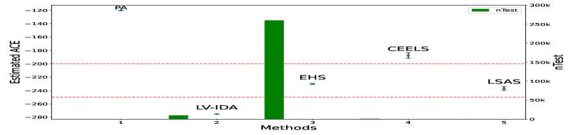
Figure 7: The causal effects and the number of (conditional) independence tests estimated by different methods, presented with 95% confidence intervals on the Cattaneo2 dataset. The two dotted lines represent the estimated interval provided in Almond et al. [2].

VI Limitations and Future Work

The preceding section presented how to locally search covariates solely from the observational data. Analogous to the setting studied by Entner et al. [10] and Cheng et al. [5], we assume that $Y$ is not a causal ancestor of $X$ and $X$ and $Y$ are not causal ancestors of any variables in $\mathbf{O}$ (pretreatment assumption). Regarding the first assumption, in practice, if one has no this prior knowledge, one can first use the existing local search structure algorithm allowing in the presence of latent variables, such as the MMB-by-MMB algorithm [47], to identify whether $Y$ is not a causal ancestor of $X$. If it is, one can still use our proposed method to search for the adjustment set and estimate the causal effect. Regarding the pretreatment assumption, though many application areas can be obtained, such as economics and epidemiology [16, 19, 43], it may not always hold in real-world scenarios. Thus, it deserves to explore methodologies that relax this assumption and address its violations. Note that some causal effects cannot be identified only based on conditional independencies among observed data. Hence, leveraging background knowledge, such as data generation mechanisms [17] and expert insights [11], to aid in identifying causal effects within local structures remains a promising research direction.

VII Conclusion

We introduce a novel local learning algorithm for covariate selection in nonparametric causal effect estimation with latent variables. Table IX summarizes the features of our method. Compared to the existing methods, our method does not require learning the global graph, is more efficient, and remains both sound and complete, even allowing for the presence of latent variables.

TABLE IX: Summary of the compared algorithm features.

Algorithm	Learning Graph	Time-complexity	Sound and Complete
LV-IDA	$\surd$	$\mathcal{O}[n\times 2^{n-1}]$ [5, 23]	$\Leftrightarrow$
EHS	$\times$	$\mathcal{O}[(n-2)\times 2^{n-2}]$	$\Leftrightarrow$
CEELS	$\times$	$\mathcal{O}\left(n\times 2^{q}\right)$	$\Rightarrow$
$LSAS$	$\times$	$\mathcal{O}[(|\mathit{MMB(X)}|-1)\times 2^{|\mathit{MMB(Y)}|-1}+2n-3]$	$\Leftrightarrow$

• Note: $\Rightarrow$ denote sound, $\Leftrightarrow$ denote sound and complete.

Acknowledgments

The authors would like to thank Debo Cheng, who kindly provided us with his R implementation of the CEELS. FX would like to acknowledge the support by the Natural Science Foundation of China (62306019). YZ would like to acknowledge the support of the Beijing Municipal Education Commission Science and Technology Program General Project (KM202410011016).

Appendix A More Examples

Example 6 (M-structure or M-bias).

As shown in Fig. 8 (a), the DAG is called M-structure (M-bias), where $U_{1}$ and $U_{2}$ are latent variables. This structure is very significant because it can lead to collider stratification bias, also known as collider bias. The MAG corresponding to this DAG is shown in Fig. 8 (b). In this graph, according to the generalized adjustment criterion, if we are interested in the causal effect between $X$ and $Y$, we should not adjust for the variable $M$. Adjusting for $M$ would open the path ($X\leftrightarrow[M]\leftrightarrow Y$), which was originally blocked. As a result, adjusting for the collider $M$ leads to over-adjustment and introduces bias.

Figure 8: The illustrative example for M-structure. (a) A causal DAG, where $U_{1}$ and $U_{2}$ are latent variables. (b) The corresponding MAG of the DAG in (a).

Appendix B Further Results on Experiments

B-A Sensitivity to Violations of the Pretreatment Assumption

In this section, we evaluate the performance of our approach on a benchmark network under conditions where the pretreatment assumption is violated.

Experimental Setup. Using the data generation mechanism outlined in the paper, we tested our approach on the MILDEW network, which comprises 35 nodes and 46 arcs. In this experiment, a pair of nodes connected by a visible edge were randomly selected as the treatment and outcome variables. Furthermore, four nodes with two or more children were randomly designated as latent variables.

Results: As shown in Table X, when the pretreatment assumption is violated, the RE metric of our method is higher compared to the case where the assumption holds (see Table VI in the paper). Nonetheless, the RE value remains relatively low, demonstrating the robustness of our algorithm even under violations of the pretreatment assumption.

TABLE X: Performance Under Violations of the Pretreatment Assumption.

	Size=2K		Size=5K		Size=7K		Size=10K
Algorithm	RE($\%$)$\downarrow$	nTest$\downarrow$	RE($\%$)$\downarrow$	nTest$\downarrow$	RE($\%$)$\downarrow$	nTest$\downarrow$	RE($\%$)$\downarrow$	nTest$\downarrow$
LSAS	22.13 ± 34.67	123.36 ± 113.43	19.26 ± 38.32	178.70 ± 382.44	15.63 ± 34.58	180.64 ± 201.86	13.75 ± 27.37	234.50 ± 427.26

• Note: $\downarrow$ means a lower value is better, and vice versa. The symbol ’-’ indicates that PA does not output this information.

B-B Sensitivity to the Number of Latent Variables

In this section, we evaluate the performance of our method as the number of latent variables increases in a benchmark network.

Experimental Setup. Using the data generation mechanism outlined in the paper, we tested our approach on the MILDEW network, which consists of 35 nodes and 46 arcs. In this setup, the node $foto4$ was chosen as the treatment variable and the node $dm4$ as the outcome variable, with the sample size set to 5K. We hid the nodes $lai4$ and $dm3$, which lie on the back-door paths from $foto4$ to $dm4$. Additionally, we randomly selected two, four, or six nodes (Num = 2, 4, or 6) with two or more children as latent variables. Note that the MILDEW network contains a total of nine nodes with two or more children.

Results: The results are summarized in Table XI. As expected, increasing the number of latent variables in the network has minimal impact on the RE metric of our method, which remains consistently low. These results demonstrate the robustness of our approach under varying levels of latent variable presence.

TABLE XI: Performance with Different Numbers of Latent Variables.

	Num=2		Num=4		Num=6
Algorithm	RE($\%$)$\downarrow$	nTest$\downarrow$	RE($\%$)$\downarrow$	nTest$\downarrow$	RE($\%$)$\downarrow$	nTest$\downarrow$
LSAS	8.03 ± 10.42	62.13 ± 6.42	8.83 ± 30.32	58.09 ± 9.46	9.04 ± 8.71	56.86 ± 4.24

• Note: $\downarrow$ means a lower value is better, and vice versa. The symbol ’-’ indicates that PA does not output this information.

References

- Agrawal et al. [1994] R. Agrawal, R. Srikant et al., “Fast algorithms for mining association rules,” in Proc. 20th int. conf. very large data bases (VLDB), vol. 1215. Santiago, 1994, pp. 487–499.
- Almond et al. [2005] D. Almond, K. Y. Chay, and D. S. Lee, “The costs of low birth weight,” The Quarterly Journal of Economics, vol. 120, no. 3, pp. 1031–1083, 2005.
- Bühlmann et al. [2010] P. Bühlmann, M. Kalisch, and M. H. Maathuis, “Variable selection in high-dimensional linear models: partially faithful distributions and the pc-simple algorithm,” Biometrika, vol. 97, no. 2, pp. 261–278, 2010.
- Cattaneo [2010] M. D. Cattaneo, “Efficient semiparametric estimation of multi-valued treatment effects under ignorability,” Journal of Econometrics, vol. 155, no. 2, pp. 138–154, 2010.
- Cheng et al. [2022] D. Cheng et al., “Local search for efficient causal effect estimation,” IEEE Transactions on Knowledge and Data Engineering, 2022.
- Cheng et al. [2023a] D. Cheng et al., “Toward unique and unbiased causal effect estimation from data with hidden variables,” IEEE transactions on neural networks and learning systems, vol. 34, no. 9, pp. 6108–6120, 2023.
- Cheng et al. [2024] D. Cheng et al., “Data-driven causal effect estimation based on graphical causal modelling: A survey,” ACM Computing Surveys, vol. 56, no. 5, pp. 1–37, 2024.
- Chu et al. [2021] Z. Chu, S. L. Rathbun, and S. Li, “Graph infomax adversarial learning for treatment effect estimation with networked observational data,” in Proceedings of the 27th ACM SIGKDD Conference on Knowledge Discovery & Data Mining, 2021, pp. 176–184.
- De Luna et al. [2011] X. De Luna, I. Waernbaum, and T. S. Richardson, “Covariate selection for the nonparametric estimation of an average treatment effect,” Biometrika, vol. 98, no. 4, pp. 861–875, 2011.
- Entner et al. [2013] Doris Entner, Patrik Hoyer, and Peter Spirtes. Data-driven covariate selection for nonparametric estimation of causal effects. In Artificial intelligence and statistics, pages 256–264. PMLR, 2013.
- Fang and He [2020] Z. Fang and Y. He, “Ida with background knowledge,” in Conference on Uncertainty in Artificial Intelligence. PMLR, 2020, pp. 270–279.
- Häggström [2018] J. Häggström, “Data-driven confounder selection via markov and bayesian networks,” Biometrics, vol. 74, no. 2, pp. 389–398, 2018.
- Häggström et al. [2015] J. Häggström, E. Persson, I. Waernbaum, and X. de Luna, “Covsel: An r package for covariate selection when estimating average causal effects,” Journal of Statistical Software, vol. 68, pp. 1–20, 2015.
- Henckel et al. [2022] L. Henckel, E. Perković, and M. H. Maathuis, “Graphical criteria for efficient total effect estimation via adjustment in causal linear models,” Journal of the Royal Statistical Society Series B: Statistical Methodology, vol. 84, no. 2, pp. 579–599, 2022.
- Hernán and Robins [2006] M. A. Hernán and J. M. Robins, “Estimating causal effects from epidemiological data,” Journal of Epidemiology & Community Health, vol. 60, no. 7, pp. 578–586, 2006.
- Hill [2011] J. L. Hill, “Bayesian nonparametric modeling for causal inference,” Journal of Computational and Graphical Statistics, vol. 20, no. 1, pp. 217–240, 2011.
- Hoyer et al. [2008] P. O. Hoyer, S. Shimizu et al., “Estimation of causal effects using linear non-Gaussian causal models with hidden variables,” International Journal of Approximate Reasoning, vol. 49, no. 2, pp. 362–378, 2008.
- Hyttinen et al. [2015] A. Hyttinen, F. Eberhardt, and M. Järvisalo, “Do-calculus when the true graph is unknown,” in Proceedings of the Thirty-First Conference on Uncertainty in Artificial Intelligence, 2015, pp. 395–404.
- Imbens and Rubin [2015] G. W. Imbens and D. B. Rubin, “Causal inference for statistics, social, and biomedical sciences: An introduction.” Cambridge University Press, 2015.
- Kalisch et al. [2012] M. Kalisch, M. Mächler, D. Colombo, M. H. Maathuis, and P. Bühlmann, “Causal inference using graphical models with the r package pcalg,” Journal of statistical software, vol. 47, pp. 1–26, 2012.
- Maathuis and Colombo [2015] M. H. Maathuis and D. Colombo, “A generalized back-door criterion,” The Annals of Statistics, vol. 43, no. 3, pp. 1060–1088, 2015.
- Maathuis et al. [2009] M. H. Maathuis, M. Kalisch, and P. Bühlmann, “Estimating high-dimensional intervention effects from observational data,” The Annals of Statistics, vol. 37, no. 6A, pp. 3133–3164, 2009.
- Malinsky and Spirtes [2016] D. Malinsky and P. Spirtes, “Estimating causal effects with ancestral graph markov models,” in Conference on Probabilistic Graphical Models. PMLR, 2016, pp. 299–309.
- Malinsky and Spirtes [2017] D. Malinsky and P. Spirtes, “Estimating bounds on causal effects in high-dimensional and possibly confounded systems,” International Journal of Approximate Reasoning, vol. 88, pp. 371–384, 2017.
- Pearl [1993] J. Pearl, “Comment: graphical models, causality and intervention,” Statistical Science, vol. 8, no. 3, pp. 266–269, 1993.
- Pearl [2009] J. Pearl, Causality. Cambridge University Press, 2009.
- Pellet and Elisseeff [2008a] J.-P. Pellet and A. Elisseeff, “Finding latent causes in causal networks: an efficient approach based on Markov blankets,” Advances in Neural Information Processing Systems, vol. 21, 2008.
- Pellet and Elisseeff [2008b] J.-P. Pellet and A. Elisseeff, “Using Markov blankets for causal structure learning.” Journal of Machine Learning Research, vol. 9, no. 7, 2008.
- Perkovi et al. [2018] E. Perkovi, J. Textor, M. Kalisch, M. H. Maathuis et al., “Complete graphical characterization and construction of adjustment sets in Markov equivalence classes of ancestral graphs,” Journal of Machine Learning Research, vol. 18, no. 220, pp. 1–62, 2018.
- Perkovic et al. [2017] E. Perkovic, M. Kalisch, and M. H. Maathuis, “Interpreting and using cpdags with background knowledge,” in Proceedings of the 24th Conference on Uncertainty in Artificial Intelligence, UAI 2017. AUAI Press, 2017.
- Peters et al. [2017] J. Peters, D. Janzing, and B. Schölkopf, Elements of Causal Inference. MIT Press, 2017.
- Richardson [2003] T. Richardson, “Markov properties for acyclic directed mixed graphs,” Scandinavian Journal of Statistics, vol. 30, no. 1, pp. 145–157, 2003.
- Richardson and Spirtes [2002] T. Richardson and P. Spirtes, “Ancestral graph markov models,” The Annals of Statistics, vol. 30, no. 4, pp. 962–1030, 2002.
- Rotnitzky and Smucler [2020] A. Rotnitzky and E. Smucler, “Efficient adjustment sets for population average causal treatment effect estimation in graphical models,” Journal of Machine Learning Research, vol. 21, no. 188, pp. 1–86, 2020.
- Rubin [1974] D. B. Rubin, “Estimating causal effects of treatments in randomized and nonrandomized studies.” Journal of educational Psychology, vol. 66, no. 5, p. 688, 1974.
- Runge [2021] J. Runge, “Necessary and sufficient graphical conditions for optimal adjustment sets in causal graphical models with hidden variables,” Advances in Neural Information Processing Systems, vol. 34, pp. 15 762–15 773, 2021.
- Shpitser et al. [2010] I. Shpitser, T. VanderWeele, and J. M. Robins, “On the validity of covariate adjustment for estimating causal effects,” in Proceedings of the 26th Conference on Uncertainty in Artificial Intelligence, UAI 2010. AUAI Press, 2010, pp. 527–536.
- Spirtes and Glymour [1991] P. Spirtes and C. Glymour, “An algorithm for fast recovery of sparse causal graphs,” Social science computer review, vol. 9, no. 1, pp. 62–72, 1991.
- Spirtes et al. [2000] P. Spirtes, C. Glymour, and R. Scheines, Causation, Prediction, and Search. MIT press, 2000.
- Textor and Liśkiewicz [2011] J. Textor and M. Liśkiewicz, “Adjustment criteria in causal diagrams: an algorithmic perspective,” in Proceedings of the Twenty-Seventh Conference on Uncertainty in Artificial Intelligence, 2011, pp. 681–688.
- Van der Zander et al. [2014] B. Van der Zander, M. Liskiewicz, and J. Textor, “Constructing separators and adjustment sets in ancestral graphs.” in CI@ UAI, 2014, pp. 11–24.
- Vander Weele and Shpitser [2011] T. J. Vander Weele and I. Shpitser, “A new criterion for confounder selection,” Biometrics, vol. 67, no. 4, pp. 1406–1413, 2011.
- Wager and Athey [2018] S. Wager and S. Athey, “Estimation and inference of heterogeneous treatment effects using random forests,” Journal of the American Statistical Association, vol. 113, no. 523, pp. 1228–1242, 2018.
- Wang et al. [2023] T.-Z. Wang, T. Qin, and Z.-H. Zhou, “Estimating possible causal effects with latent variables via adjustment,” in International Conference on Machine Learning. PMLR, 2023, pp. 36 308–36 335.
- Witte et al. [2020] J. Witte, L. Henckel, M. H. Maathuis, and V. Didelez, “On efficient adjustment in causal graphs,” Journal of Machine Learning Research, vol. 21, no. 246, pp. 1–45, 2020.
- Wu et al. [2022] A. Wu, J. Yuan, K. Kuang et al., “Learning decomposed representations for treatment effect estimation,” IEEE Transactions on Knowledge and Data Engineering, vol. 35, no. 5, pp. 4989–5001, 2022.
- Xie et al. [2024] F. Xie, Z. Li, P. Wu, Y. Zeng, L. Chunchen, and Z. Geng, “Local causal structure learning in the presence of latent variables,” in Forty-first International Conference on Machine Learning, 2024.
- Zhang [2008a] J. Zhang, “Causal reasoning with ancestral graphs.” Journal of Machine Learning Research, vol. 9, no. 7, 2008.
- Zhang [2008b] J. Zhang, “On the completeness of orientation rules for causal discovery in the presence of latent confounders and selection bias,” Artificial Intelligence, vol. 172, no. 16-17, pp. 1873–1896, 2008.
- Yu [2018] K. Yu et al., “Mining markov blankets without causal sufficiency,” IEEE transactions on neural networks and learning systems, vol. 29, no. 12, pp. 6333–6347, 2018.