Dynamics and modulation of cosmic ray modified magnetosonic waves in a galactic gaseous rotating plasma

Abstract

The influence of the presence of cosmic fluid on the magnetosonic waves and modulation instabilities in the interstellar medium of spiral galaxies is investigated. The fluid model is developed by modifying the pressure equation in such dissipative rotating magnetoplasmas incorporating thermal ionized gas and cosmic rays. Applying the normal mode analysis, a modified dispersion relation is derived to study linear magnetosonic wave modes and their instabilities. The cosmic rays influence the wave damping by accelerating the damping rate. The standard reductive perturbation method is employed in the fluid model leading to a Korteweg–de Vries-Burgers (KdVB) equation in the small-amplitude limit. Several nonlinear wave shapes are assessed by solving the KdVB equation, analytically and numerically. The cosmic ray diffusivity and magnetic resistivity are responsible for the generation of shock waves. The modulational instability (MI) and the rogue wave solutions of the magnetosonic waves are studied by deriving a nonlinear Schrödinger (NLS) equation from the obtained KdVB equation under the assumption that the cosmic ray diffusion and magnetic resistivity are weak and the carrier wave frequency is considerably lower than the wave frequency. The influence of various plasma parameters on the growth rate of MI is examined. The modification of the pressure term due to cosmic fluid reduces the MI growth in the interstellar medium. In addition, a quantitative analysis of the characteristics of rogue wave solutions is presented. Our investigation’s applicability to the interstellar medium of spiral galaxies is traced out.

I INTRODUCTION

In our Galaxy, interstellar medium (ISM) clouds are highly inhomogeneous and comprise various phases of gas clouds, such as a hot phase, a warm phase, diffusive clouds, molecular clouds, etc. These components of the ISM cloud exhibit a similar energy density distributionkuwabara2020dynamics . It is well-known that the galactic cosmic rays significantly contribute to the evolution and structure formation of ISM clouds. Galactic cosmic rays parker1969galactic ; padovani2020impact are highly energetic particles ejected from astrophysical bodies outside our solar system, such as supernova remnants, planetary disks, the Sun, etc., which numerously interact with different components of the ISM. Cosmic rays play an important role in the charge of dust grains kalvans2016temperature , gas ionization yusef2007cosmic , and energy transfer gaches2019astrochemical in the interstellar medium. They interact with cosmic dust grains via different physical mechanisms, leading to the generation of different wave modes and instabilities in the media. They are major contributors to the ionization of molecular clouds (MCs) core padovani2011effects and the ionization of molecule hydrogen ($H_{2}$) in diffuse interstellar clouds indriolo2009implications . They transfer energy to the dust grains through heating the dust grains in cosmic ray-plasma interactions.

The nonlinearities in the plasma contribute to energy localization, leading to the evaluation of various kinds of nonlinear coherent structures, like solitons, shocks, etc., which have immense application in space as well as astrophysical plasma environmentsgoertz1989dusty ; havnes1992charged ; horanyi1986effects . The evolutions of these nonlinear coherent structures are characterized by various well-known nonlinear partial differential equations, such as Korteweg-de Vries (KdV) and KdV-like equations wazwaz2017abundant , the Zakharov-Kuznetsov (ZK) and ZK-like equations, and Kadomtsev-Petviashvili (KP) and KP-like equations chen2018special ; el2016generation . Another crucial equation that controls the motion of nonlinear structures is the nonlinear Schrödinger (NLS) equationmihalache2017multidimensional . A rogue waveakhmediev2009waves ; muller2005rogue is one of the viable rational solutions of the NLS equationsharma2024modulation ; chen2015vector . Such waves are often referred to as monster, violent, extreme, or giant waves that have a few times higher amplitude than solitary waves and are observed in coastal waters kharif2008rogue , fibre optic and optical systems solli2007optical , Bose-Einstein condensates bludov2009matter , atmosphere stenflo2010rogue and astrophysical environments sabry2012freak . There has been increasing interest in investigating the behaviour of magnetosonic waves and the associated coherent structures like solitons, shocks, rogue waves, etc., in different plasma environmentsrahim2019magnetosonic ; hager2023magnetosonic ; el2012rogue ; moslem2011surface ; akbari2014electrostatic .

In recent times, researchers have devoted significant attention to the role of cosmic rays in various wave modes in linear regimes and their stability/instabilities. In this direction, Turi and Misra turi2022magnetohydrodynamic have addressed the impact of cosmic rays on the propagation of MHD waves as well as their instability (Jeans) for a self-gravitating galactic gaseous cloud. In another work, Boro and Prajapati boro2023cosmic have studied the Jeans instability for the molecular dusty plasma environment of molecular clouds, including cosmic rays. Further, various previous studies suggest that the Coriolis force plays an important role in various plasma phenomena in different plasma environments, like rotating plasma in the laboratory as well as astrophysical plasmaturi2022magnetohydrodynamic ; hager2023magnetosonic . To the best of our knowledge, the influence of cosmic rays on the dynamics of nonlinear coherent structures in ISM clouds, under the effect of Coriolis force, has not yet been addressed. Thus, in the current work, we aim to explore the impact of cosmic rays on linear and nonlinear magnetosonic shocks, solitons, and rogue waves in a dissipative rotating magnetoplasma consisting of thermal gas and cosmic rays. The present model is suitable and well justified in real physical situations like ISM clouds in spiral galaxies. For a fairly good approximation in studying the structures and evolution of this system, a hydrodynamic description including the cosmic rays has been considered.

This present work is organised as follows: in Sec. II, we describe the basic equations for the MHD waves. In Sec. III, linear properties of the magnetosonic waves are discussed through the linear dispersion relation. Sec. IV includes nonlinear analysis, where we derive a Korteweg–de Vries–Burgers (KdVB) equation for the magnetosonic waves and analyse the analytical and numerical behaviour of the equation. Sec. V is devoted to modulational instability and rogue wave solutions for carrier wave frequencies much smaller than the wave frequency. Finally, we summarize our main findings in Sec. VI.

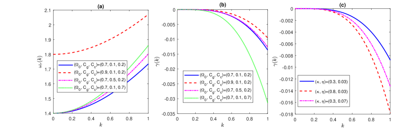
Figure 1: The real part $\omega_{r}\equiv\omega_{r}(k)$ and the damping rate $\gamma\equiv\gamma_{(}k)$ of the dispersion relation (15) are displayed for different values of the parameters as mentioned in the legends. Here, ($\theta$, $\kappa$, $\eta$)= ($\pi/3,0.3,0.03)$ in the subplots (a) & (b) and $(\theta,\Omega_{0},C_{g},C_{c})=(\pi/3,0.9,0.2,0.4)$ in the subplot (c). The other parameter values are $\rho_{0}\sim 10^{-21}Kg/m^{3}$, $B_{0}\sim 1$ nT, $P_{g0},P_{c0}\sim 10^{-13}N/m^{2}$, $\eta\sim 0.4(V_{A}^{2}/\omega_{ci})s^{-1}$ and $\kappa\sim 0.06(V_{A}^{2}/\omega_{ci})s^{-1}$.

II BASIC EQUATIONS OF THE PROBLEM

The typical plasma environment of the interstellar medium, composed of ionized thermal gas and cosmic rays, has been considered for the study of the propagation of magnetosonic waves. Here, the thermal ionized gas is considered polytropic, having no diffusion in any direction, and cosmic rays are assumed to be gas with negligible density but contributing significantly to the pressure of the system bonanno2008generation ; turi2022magnetohydrodynamic . The plasma is supposed to be immersed in a uniform external magnetic field $\mathbf{B}=B(x,t)\hat{e}_{z}$, where $B(x,t)$ is the static external magnetic field strength and $\hat{e}_{z}$ denotes the unit vector along the $z$ direction. The environment of the interstellar medium is considered to be homogeneous, fully ionized, and highly conductive fluid with a higher Reynold’s number. The plasma system is assumed to rotate slowly with a rotational frequency $\Omega$ around an axis lying in the $xz$-plane. The basic evolution equations describing the dynamics of magnetosonic waves are given as turi2022magnetohydrodynamic

$$\frac{\partial\rho}{\partial t}+\mathbf{\nabla}\cdot\left(\rho\mathbf{v}\right)=0,$$ (1)

$$\frac{\partial\mathbf{v}}{\partial t}+\left(\mathbf{v}\cdot\mathbf{\nabla}\right)\mathbf{v}=-\frac{1}{\rho}\mathbf{\nabla}\left(P+\frac{\mathbf{B}^{2}}{2\mu_{0}}\right)\\ +\frac{1}{\rho\mu_{0}}\left(\mathbf{B}\cdot\mathbf{\nabla}\right)\mathbf{B}-2\mathbf{\Omega}\times\mathbf{v},$$ (2)

$$\frac{\partial\mathbf{B}}{\partial t}+\left(\mathbf{v}\cdot\mathbf{\nabla}\right)\mathbf{B}=\left(\mathbf{\textbf{B}}\cdot\mathbf{\nabla}\right)\mathbf{v}-\left(\mathbf{\nabla}\cdot\mathbf{v}\right)\mathbf{B}+\eta\mathbf{\nabla^{2}B},$$ (3)

where $\rho$ and $\mathbf{v}$ denote the fluid (thermal gas) mass density and velocity, respectively, $\mu_{0}$ is the vacuum permittivity, and $\eta$ is the coefficient of the magnetic resistivity. The total pressure is given by $P=P_{g}+P_{c}$ where $P_{g}$ and $P_{c}$ are the gas pressure and the pressure due to the cosmic rays, respectively. As the fluid is assumed to be a thermal gas which behaves adiabatically, we use the following equation of state,

$$\frac{\partial P_{g}}{\partial t}+\mathbf{v}\cdot\mathbf{\nabla}P_{g}+\gamma_{g}\mathbf{\nabla}\cdot\mathbf{v}=0,$$ (4)

where $\gamma_{g}$ is the specific heat ratio of the thermal gas. The diffusion convection equation for cosmic rays is given by zank1990weakly

$$\frac{\partial P_{c}}{\partial t}+\mathbf{v}\cdot\mathbf{\nabla}P_{c}+\gamma_{c}\mathbf{\nabla}\cdot\mathbf{v}-\kappa\mathbf{\nabla}^{2}P_{c}=0,$$ (5)

where $\gamma_{c}$ is the adiabatic index corresponding to cosmic rays, assumed to be a constant, and $\kappa$ is the hydrodynamic form of the diffusion coefficient.

The magnetosonic waves are assumed to propagate along the $x$-direction, magnetic fields are supposed to be along $z$-direction and the plasma is slowly rotating around an axis making an angle $\theta$ with $z$ the axis. Thus, by replacing $\mathbf{\nabla}$ by $(\frac{\partial}{\partial x},0,0)$, $\mathbf{v}$ by $(v_{x},v_{y},v_{z})$ and $\mathbf{\Omega}$ by $(\Omega_{0}\sin\theta,0,\Omega_{0}\cos\theta)$, we rewrite the basis Eqs. (1)-(5) as follows

$$\frac{\partial\rho}{\partial t}+\frac{\partial}{\partial t}\left(\rho v_{x}\right)=0,$$ (6)

$$\rho\left(\frac{\partial v_{x}}{\partial t}+v_{x}\frac{\partial v_{x}}{\partial x}\right)=\frac{\partial P_{g}}{\partial x}-\frac{\partial P_{c}}{\partial x}-B\frac{\partial B}{\partial x}+2\rho\Omega_{0}\cos\theta v_{y},$$ (7)

$$\frac{\partial v_{y}}{\partial t}+v_{x}\frac{\partial v_{y}}{\partial x}=2(\Omega_{0}\sin\theta v_{z}-\Omega_{0}\cos\theta v_{x}),$$ (8)

$$\frac{\partial v_{z}}{\partial t}+v_{x}\frac{\partial v_{z}}{\partial x}=-2\Omega_{0}\sin\lambda v_{y},$$ (9)

$$\frac{\partial B}{\partial t}+\frac{\partial}{\partial x}\left(v_{x}B\right)=\eta\frac{\partial^{2}B}{\partial x^{2}},$$ (10)

$$\frac{\partial P_{g}}{\partial t}+v_{x}\frac{\partial}{\partial x}P_{g}+\gamma_{g}P_{g}\frac{\partial v_{x}}{\partial x}=0,$$ (11)

$$\frac{\partial P_{c}}{\partial t}+v_{x}\frac{\partial}{\partial x}P_{c}+\gamma_{c}P_{c}\frac{\partial v_{x}}{\partial x}-\kappa\frac{\partial^{2}P_{c}}{\partial x^{2}}=0.$$ (12)

The above set of Eqs. (6)-(12) is made normalized by normalising the variables and parameters as follows: $\rho\rightarrow\rho/\rho_{0}$, $B\rightarrow B/B_{0}$, $t\rightarrow t\omega_{ci}$, $v_{x}\rightarrow v_{x}/V_{A}$, $v_{y}\rightarrow v_{y}/V_{A}$, $v_{z}\rightarrow v_{z}/V_{A}$, $x\rightarrow x\omega_{ci}/V_{A}$, $\Omega\rightarrow\Omega/\omega_{ci}$, $P_{g}\rightarrow P_{g}/\rho_{0}V_{A}^{2}$, $P_{c}\rightarrow P_{c}/\rho_{0}V_{A}^{2}$, $\eta\rightarrow\eta\omega_{ci}/V_{A}^{2}$, $\kappa\rightarrow\kappa\frac{\omega_{ci}}{V_{A}^{2}}$, where, $\rho_{0}$ is the equilibrium density, $B_{0}$ is the equilibrium magnetic field strength, and $\omega_{ci}=\frac{eB_{0}}{m_{i}}$ is the ion cyclotron frequency, $V_{A}=\frac{B_{0}}{\sqrt{\mu_{0}\rho_{0}}}$ is the Alfvén velocity. Furthermore, our analysis is suitable based on real magnetoplasma systems, which are desired to be relevant in spiral galaxies gliddon1966gravitational ; turi2022magnetohydrodynamic . Consequently, for numerical demonstration, we choose the typical consistent parameter values as $B_{0}\sim 1$ nT, $\rho_{0}\sim 10^{-21}$ Kg/m³, $P_{g0}\sim 10^{-13}$ N/m², $P_{c0}\sim 10^{-13}$N/m² and the other parameters are taken as $\eta\sim 10^{-1}V_{A}^{2}/\omega_{ci}$, $\kappa\sim 10^{-2}V_{A}^{2}/\omega_{ci}$. In this regime, the ion gyro-frequency is typically scaled as $\omega_{ci}\sim 10^{-1}$ s^-1. The numerical value of the rotational frequency is taken to be much lower than the ion gyro-frequency $\omega_{ci}$ abdikian2022drift .

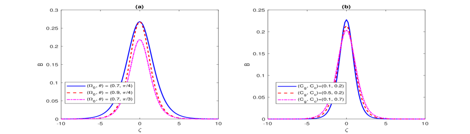
Figure 2: One-soliton profiles $B~{}\text{vs}~{}\zeta$ are plotted for different values of the parameters as mentioned in the legends. Here, $(C_{g},C_{c})$= $(0.2,0.4)$ and $(\Omega_{0},\theta)=(0.9,\pi/3)$ in the subplots (a) and (b), respectively, and $v_{0}=0.1$. The other parameters remain unchanged as in Fig. 1.

III LINEAR ANALYSIS

We study the propagation of magnetosonic plane waves in this plasma system along the $x$-direction. To proceed, we linearize the set of Eqs. (6)-(12) about the equilibrium state by assuming the plasma is uniform with constant density and zero velocity. Dividing the physical quantity $f$ into the equilibrium ($f_{0}$) and perturbed ($f_{1}$) parts as $f=f_{0}+f_{1}$, where $f=(\rho,B,v_{x},v_{y},v_{z},P_{g},P_{c})$, $f_{0}=(1,1,0,0,0,P_{g0},P_{c0})$ and $f_{1}=(\rho_{1},B_{1},v_{x1},v_{y1},v_{z1},P_{g1},P_{c1})$, we obtain a linearized set of equations from Eqs. (6)-(12).

Assuming the perturbations to vary as a plane wave of the form $\sim exp\left(ikx-i\omega t\right)$ with wave number $k$ and wave frequency $\omega$, we get the following linear dispersion relation

$$\omega^{2}=\left(C_{g}^{2}+C_{c}^{2}\frac{\omega}{\omega+i\kappa k^{2}}+\frac{\omega}{\omega+i\eta k^{2}}\right)k^{2}$$

$$+\frac{4\Omega_{0}^{2}\cos^{2}\theta\omega^{2}}{(\omega^{2}-4\Omega_{0}^{2}\sin^{2}\theta)},$$ (13)

where $C_{g}(=\sqrt{\gamma_{g}P_{g0}})$ and $C_{c}(=\sqrt{\gamma_{c}P_{c0}})$ are the normalized form (normalized by $V_{A}$) of the speed of thermal gas and cosmic rays, respectively. It is worth mentioning that the denormalization of the above quantities yields $C_{g}=\sqrt{\frac{\gamma_{g}P_{g0}}{\rho_{0}}}$ and $C_{c}=\sqrt{\frac{\gamma_{c}P_{c0}}{\rho_{0}}}$. The dispersion relation (III) agrees with a similar result as in Ref. turi2022magnetohydrodynamic in the absence of magnetic resistivity ($\eta$) and cosmic ray diffusivity ($\kappa$). Due to the presence of the parameters $\eta$ and $\kappa$ in the dispersion relation, $\omega$ and $k$ become complex. The dispersion is also influenced by the rotational frequency ($\Omega_{0}$) and the angle $\theta$ related to the rotation of the fluid in the $xz$-plane. If the axis of rotation is taken along $x$-axis (i.e. $\theta=\pi/2$), the dispersion relation (III) modified to

$$\omega^{2}=\left(C_{g}^{2}+C_{c}^{2}\frac{\omega}{\omega+i\kappa k^{2}}+\frac{\omega}{\omega+i\eta k^{2}}\right)k^{2},$$ (14)

where the effects of the Coriolis force disappear due to the rotation of the plasma along the $x$-axis, however, the influences of magnetic resistivity and cosmic ray diffusivity have been retained. The wave becomes dispersionless in long-wavelength limits (i.e. when $k\ll 1$) and/or when the effects of magnetic resistivity and cosmic ray diffusivity weaken and the dispersion reduces to $\omega=ak$ where $a=(1+C_{g}^{2}+C_{c}^{2})^{1/2}$. In the case of when the axis of rotation is taken along the $z$-axis (i.e. $\theta=0$), the dispersion relation (III) reduces to

$$\omega^{2}=\left(C_{g}^{2}+C_{c}^{2}\frac{\omega}{\omega+i\kappa k^{2}}+\frac{\omega}{\omega+i\eta k^{2}}\right)k^{2}+4\Omega_{0}^{2}.$$ (15)

The dispersion (15) includes the effect of the Coriolis force due to the rotation of the plasma. The wave becomes unstable because of the presence of cosmic rays and magnetic diffusion, i.e., it can be either damped or anti-damped. To obtain the growth rate (or damping) we separate the real and imaginary parts of the wave frequency as $\omega=\omega_{r}+i\gamma$ with the assumption $|\gamma|$, $|\kappa|$, $|\eta|\ll\omega_{r}$, $\frac{\omega}{\omega+i\kappa k^{2}}\approx(1-i\frac{\kappa k^{2}}{\omega_{1}})$ and $\frac{\omega}{\omega+i\eta k^{2}}\approx(1-i\frac{\eta k^{2}}{\omega_{1}})$, where $\omega_{1}$ is the solution of Eq. (15) at $\eta=\kappa=0$. We found that the magnetosonic wave gets damped, and the absolute value of damping is estimated to be $|\gamma|\sim\frac{1}{2}(C_{c}^{2}\kappa+\eta)\frac{k^{4}}{\omega_{1}^{2}}$ and the real part is $\omega_{r}=\omega_{1}$.

To study the dispersion and damping characteristic of the magnetosonic wave, we take numerical results from Eq. (15) displayed in Fig. 1. The plots of the real part $\omega_{r}=\omega_{r}(k)$ are shown in the subplot (a) for different values of the parameters $\Omega_{0}$, $C_{g}$ and $C_{c}$ associated with the rotational frequency, thermal pressure and cosmic ray pressure, respectively. It is found that initially, for $k\ll 1$, the profile of $\omega_{r}$ remains parallel to the axis of wave number, i.e., the phase velocity approaches a constant value, as we discussed earlier. Beyond the limit $k\ll 1$, the frequency of the wave increases with increasing values of $k$. The profiles ($\omega_{r}$) are plotted for four sets of values of $\Omega_{0}$, $C_{g}$ and $C_{c}$. It has been observed from the profiles that an increase in either of these three parameters, keeping the values of alternate parameters fixed, leads to an enhancement of the wave frequency. However, in the limit $k\ll 1$, the increases in wave frequencies are found to be negligible for increasing values of $C_{g}$ and $C_{c}$, beyond the limit, the increments are transpicuous. In the subplots (b) and (c) of Fig. 1, the profiles of estimated damping rate $\gamma=\gamma(k)$ are plotted for different values of $\Omega_{0}$, $C_{g}$, $C_{c}$ and $\kappa$, $\eta$, respectively. The figures show that the absolute damping rate is negligible in the limit $k\ll 1$ but the damping grows with increasing values of $k$. Subplot (b) depicts that an increase in the values of $\Omega_{0}$ and $C_{g}$ decreases the absolute damping rate, whereas the wave damping increases with increasing value of the parameter $C_{c}$. On the other hand, from the subplot (c), the significant growth in the damping rate has been noticed with the increasing values of $\eta$ and $\kappa$, which leads to unstable behaviour in the system. Magnetic resistivity $\eta$ and cosmic ray diffusivity $\kappa$ do not contribute to the real part of the wave frequency but influence the wave damping. However, subplots (a) and (b) show that the absolute damping $\gamma$ reduces as the rotating frequency increases, but the real part of the wave frequency increases. So, it is interesting to note that the damping due to magnetic resistivity and cosmic ray diffusivity becomes insignificant with an increase in rotating frequency.

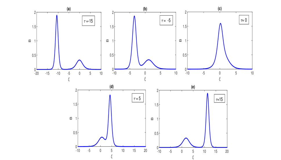
Figure 3: Two-soliton profiles $B~{}\text{vs}~{}\xi$ are displayed for different values of $\tau$. Here, $(\Omega_{0},\theta,C_{g},C_{c})=(0.7,\pi/4,0.2,0.4)$, $k_{1}=0.5$ and $k_{2}=1.2$. The other parameters remain unchanged as in Fig. 1.

IV NONLINEAR ANALYSIS

IV.1 KdVB Equation Derivation

In this section, we are interested in the non-linear evolution of progressive shocks of the one-dimensional plane in a frame that moves along the $x$-axis with the wave phase velocity. For this purpose, we derive an evolution equation for small-amplitude shocks and study their characteristics in physical parameter space. To employ the standard reductive perturbation technique, we stretch the space and time coordinates,

$$\xi=\epsilon^{1/2}(x-\lambda t),\tau=\epsilon^{3/2}t,$$ (16)

where $\lambda$ is the wave’s phase velocity and the parameter $\epsilon$ measures the weakness of the nonlinearity. We expand the dependent variables in terms of $\epsilon$ as hager2023magnetosonic

$$\rho=1+\epsilon\rho_{1}+\epsilon^{2}\rho_{2}+\dots,$$

$$v_{x}=0+\epsilon v_{x1}+\epsilon^{2}v_{x2}+\dots,$$

$$v_{z}=0+\epsilon v_{y1}+\epsilon^{2}v_{y2}+\dots,$$

$$B=1+\epsilon B_{1}+\epsilon^{2}B_{2}+\dots,$$ (17)

$$P_{g}=P_{g0}+\epsilon P_{g1}+\epsilon^{2}P_{g2}+\dots,$$

$$P_{c}=P_{c0}+\epsilon P_{c1}+\epsilon^{2}P_{c2}+\dots,$$

while $v_{y}$ is expressed as

$$v_{y}=0+\epsilon^{3/2}v_{y1}+\epsilon^{5/2}v_{y2}+\dots.$$ (18)

. Furthermore, we assume that $\eta\sim\eta_{0}\epsilon^{1/2}$ and $\kappa\sim\kappa_{0}\epsilon^{1/2}$ to make the perturbation evolution equation consistent, where $\eta_{0}$ and $\kappa_{0}$ are of the order of unity. The parameters $\eta$ and $\kappa$ are expanded in the lowest order of $\epsilon$ to take into account their effects for the propagation of dissipative magnetosonic shock waves numerically, which are valid as resistive and diffusive terms in Eq. (10) and (12), respectively, are almost linearly proportional to the number density. Similar assumptions have been made previously in many experimental situations nakamura1999observation ; nakamura2001observation . For large values of $\eta_{0}$ and $\kappa_{0}$, one can choose a higher order of $\epsilon$ (i.e., $\eta\sim\epsilon\eta_{0}$, $\kappa\sim\epsilon\kappa_{0}$) and in those cases sharp rising shock waves are noticed compared to oscillatory and monotonic shock waves (for $\eta\sim\epsilon^{1/2}\eta_{0}$, $\kappa\sim\epsilon^{1/2}\kappa_{0}$).

Inserting the stretched coordinates (16), the expressions (17) and (18) into the Eqs. (6) to (12), we identify the different powers of $\epsilon$. From the lowest order of $\epsilon$, we obtain the following expressions:

$$v_{x1}=\lambda\rho_{1}=\lambda B_{1},P_{g1}=C_{g}^{2}B_{1},v_{z1}=\lambda\cot\theta B_{1}$$

$$P_{c1}=C_{c}^{2}B_{1},v_{y1}=\frac{\lambda^{2}}{2\Omega_{0}}\frac{\cot\theta}{\sin\theta}\frac{\partial B_{1}}{\partial\xi},$$ (19)

together with the compatible condition,

$$\lambda^{2}=(1+C_{g}^{2}+C_{c}^{2})\times\frac{1}{(1+\cot^{2}\theta)}.$$ (20)

Similarly, we obtain a system of equations in the next order of $\epsilon$. Eliminating those perturbed quantities from the system and using the results given in Eq. (IV.1), we derive the following KdVB equation,

$$\frac{\partial B}{\partial\tau}+QB\frac{\partial B}{\partial\xi}+R\frac{\partial^{3}B}{\partial\xi^{2}}=S\frac{\partial^{2}B}{\partial\xi^{2}},$$ (21)

where the first-order magnetic field perturbation $B_{1}$ is replaced by $B$. The coefficient of nonlinearity $Q$, the coefficient of dispersion $R$ and the coefficient of dissipation $S$ are obtained as

$$Q=\frac{\lambda\left(3+C_{g}^{2}+C_{c}^{2}+\gamma_{g}C_{g}^{2}+\gamma_{c}C_{c}^{2}\right)}{\left(1+C_{g}^{2}+C_{c}^{2}+\lambda^{2}+\lambda^{2}\cot^{2}\theta\right)},$$ (22)

$$R=\frac{\lambda^{5}\cot^{2}\theta}{4\Omega_{0}^{2}\sin^{2}\theta}\times\frac{1}{\left(1+C_{g}^{2}+C_{c}^{2}+\lambda^{2}+\lambda^{2}\cot^{2}\theta\right)},$$ (23)

$$S=\frac{\left(\kappa_{0}C_{c}^{2}+\eta_{0}\right)}{\left(1+C_{g}^{2}+C_{c}^{2}+\lambda^{2}+\lambda^{2}\cot^{2}\theta\right)}.$$ (24)

Here, all the coefficients $Q$, $R$ and $S$ are modified due to the presence of the parameters $C_{g}$, $C_{c}$ and $\theta$ related to the effects of thermal pressure, cosmic ray pressure and axis of rotation, respectively. However, in addition to these parameters, the diffusivity of cosmic rays ($\kappa_{0}$) and the magnetic resistivity ($\eta_{0}$) affect the dissipation coefficient $S$ whereas the rotation frequency ($\Omega_{0}$) affects the dispersion coefficient $R$. In the absence of cosmic ray diffusivity ($\kappa_{0}=0$) and magnetic resistivity ($\eta_{0}=0$), Eq. (21) reduces to the well-known KdV equation, and the solution can be obtained in terms of a solitary wave pulse. In other words, the parameters $\kappa_{0}$ and $\eta_{0}$ in the present model yield the formation of shock structures. In the limiting case, $\theta=\pi/2$, the dispersion coefficient vanishes, consequently Eq. (21) reduces to the Burgers equation having a stationary shock profile. Now, we move on to find various types of soliton and shock wave solutions from Eq. (21) for different cases.

IV.2 Soliton Solutions

If the effects of cosmic ray diffusivity ($\kappa_{0}$) and magnetic resistivity ($\eta_{0}$) become negligible, one can obtain the following KdV equation, disregarding their effects from Eq. (21), as

$$\frac{\partial B}{\partial\tau}+QB\frac{\partial B}{\partial\xi}+R\frac{\partial^{3}B}{\partial\xi^{2}}=0,$$ (25)

which admits the well-known one-soliton solution given by,

$$B=\frac{3v_{0}}{Q}\mathrm{sech}\,^{2}\left[\sqrt{\frac{v_{0}}{4R}}\zeta\right]$$ (26)

where $\zeta=\xi-v_{0}\tau$ and $v_{0}$ is the speed of the travelling wave. The typical profiles of one-soliton (solitary wave pulse) are plotted in Fig. 2 for different values of plasma parameters $\Omega_{0}$, $\theta$ (in the subplot (a)) and $C_{g}$, $C_{c}$ (in the subplot (b)), respectively. The width of the wave is found to become narrower, however, the amplitude of the wave remains unchanged as the rotating frequency $\Omega_{0}$ increases. But, if the angle of rotation $\theta$ increases, the amplitude and width of the solitary wave pulse decrease. Subplot (b) shows that a small increase in thermal pressure ($C_{g}$) and cosmic ray pressure ($C_{c}$) decrease the wave amplitude, but the width of the pulse becomes wider.

$\mathrm{sech}\,{x}$ Now, we describe the transmission and interactions of two-soliton solutions for the KdV equation employing Hirota’s bilinear methodhirota1971exact . Recalling the variables $\xi$ by $\tilde{\xi}B^{1/3}$, $B$ by $6\tilde{B}{Q^{*}}^{-1}R^{1/3}$ and $\tau$ by $\tilde{\tau}$, we rewrite the KdV equation as

$$\frac{\partial\tilde{B}}{\partial\tilde{\tau}}-6\tilde{B}\frac{\partial\tilde{B}}{\partial\tilde{\xi}}+\frac{\partial^{3}\tilde{B}}{\partial\tilde{\xi^{2}}}=0.$$ (27)

where $Q^{*}=-Q$. Assuming the transformation $\tilde{B}=-2\left(\log f\right)_{\tilde{\xi}\tilde{\xi}}$, we obtain the Hirota bilinear form of Eq. (27) as

$$\left(D_{\tilde{\xi}}D_{\tilde{\tau}}+D_{\tilde{\xi}}^{4}\right)\left\{f\cdot f\right\}=0,$$ (28)

where $f=1+\epsilon\left(e^{\tilde{\theta}_{1}}+e^{\tilde{\theta}_{2}}\right)+\epsilon^{2}f_{2}$, $\tilde{\theta}_{i}=k_{i}\tilde{\xi}+\tilde{\omega}_{i}\tilde{\tau}$ ($i=1,2$) and $D$ represents Hirota’s operator. Collecting various powers of $\epsilon$ from Eq. (28), we obtain $\omega_{i}=-k_{i}^{3}$ and $f_{2}=a_{12}e^{\tilde{\theta}_{1}+\tilde{\theta}_{2}}$, with phase shift $a_{12}=\frac{(k_{1}-k_{2})^{2}}{(k_{1}+k_{2})^{2}}$. Finally, we have the two-soliton solution of Eq. (25) obtained as

$$B=-12\frac{R^{1/3}}{Q^{*}}\frac{k_{1}^{2}e^{\theta_{1}}+k_{2}^{2}e^{\theta_{2}}+a_{12}e^{\theta_{1}+\theta_{2}}(k_{2}^{2}e^{\theta_{1}}+k_{1}^{2}e^{\theta_{2}})+2(k_{1}-k_{2})^{2}e^{\theta_{1}+\theta_{2}}}{(1+e^{\theta_{1}}+e^{\theta_{2}}+a_{12}e^{\theta_{1}+\theta_{2}})^{2}}$$ (29)

, where $\theta_{i}=\frac{k_{i}}{R^{1/3}}\xi-k_{i}^{3}\tau$ ($i=1,2$) and $\tilde{B}$ is replaced by $\tilde{B}=\frac{Q^{*}B}{6R^{1/3}}$. As $\tau\gg 1$ the obtained solution (29) converts to the following superposed two individual single-soliton solutions, gradually, as followsdrazin1989solitons

$$B_{12}\sim\sum_{i=1}^{2}A_{i}\mathrm{sech}\,{\left[\frac{k_{i}}{2R^{1/3}}(\xi-k_{i}^{2}R^{1/3}\tau+\Delta_{i})\right]},$$ (30)

where $A_{i}=\frac{3R^{1/3}k_{i}^{2}}{2Q^{*}}$ ($i=1,2$) is the amplitude and the phase shifts of the solitons due to interactions are $\Delta_{1,2}=\pm\frac{2R^{1/3}\log|\frac{k_{2}-k_{1}}{k_{2}+k_{1}}|}{k_{1,2}}$.

Numerically, we demonstrate the temporal evolution and phase shift of the two-soliton solution of the KdV equation by the interaction of two solitons. In Fig. 3, the time evaluation of two solitons interactions $B$ vs. $\xi$ have been plotted for different values of $\tau$. One can observe that two solitons with different amplitudes collide and exchange energy and phase. The shape and size of both solitons may alter during collision. Fig. 3 also depicts that for $\tau<0$, the soliton with higher amplitude stays behind the lesser one and as $\tau$ increases, the two solitons get closer. Subsequently, two solitons collide at $\tau=0$ and become one-soliton, after that, the soliton with higher amplitude moves faster than the lesser one, keeping the latter one behind. We noticed that when we changed the system’s parametric values for the two-soliton solution, the characteristics framework stayed consistent with what we saw for the one-soliton solution.

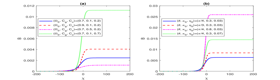
Figure 4: The magnetosonic shock profiles $B~{}\text{vs}~{}\chi$ are plotted [Eq. (38)] for different parametric values as mentioned in the legends. Here, ($\theta$, $\kappa$, $\eta$)= ($\pi/3$, 0.3, 0.03) and $(\Omega_{0},C_{g},C_{c})=(0.9,0.2,0.4)$ for the subplots (a) and (b), respectively. The other parameters remain unchanged as in Fig. 1.

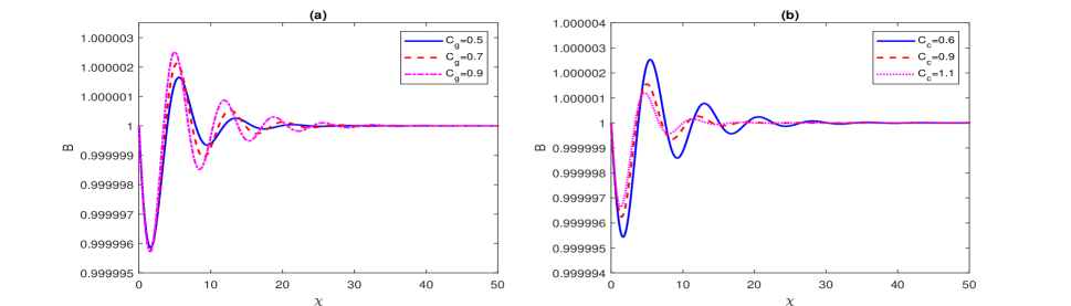
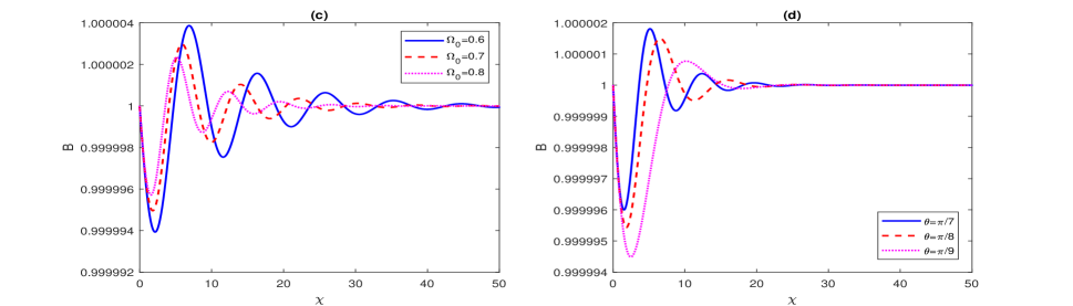
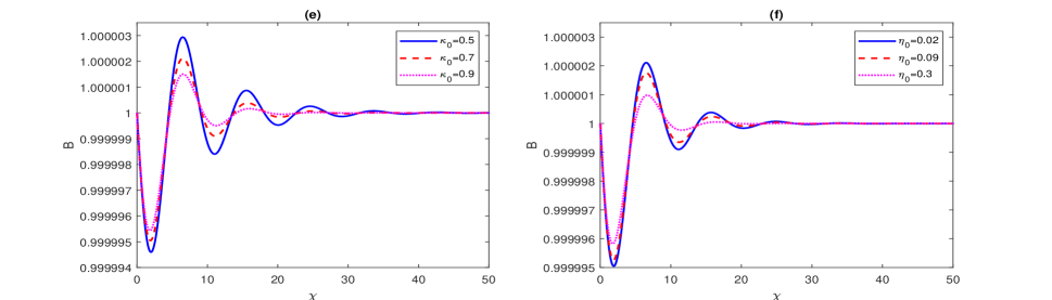
Figure 5: The magnetosonic oscillatory shock profiles $B~{}\text{vs}~{}\chi$ are plotted for different values of the parameters as mentioned in the legends. The other parameters in the subplots, except the variation parameter, are fixed as $(C_{g},C_{c},\Omega_{0},\theta,\kappa_{0},\eta_{0})=(0.7,0.6,0.8,\pi/7,0.9,0.02)$.

IV.3 Shock Wave Solutions

After that, we discuss the case in which the effects of the parameter $\kappa_{0}$ and $\eta_{0}$ are considerable, and consequently, the dissipation coefficient $S$ plays a significant role in the evaluation of the shock wave solution of the KdVB equation (21). The dispersion coefficient $R$ disappears for $\theta=\pi/2$ and, as a result, Eq. (21) reduces to the Burgers equation with a stationary shock solution ashossen2017electrostatic ,

$$B(\xi,\tau)=\frac{2U_{0}}{Q}\left[1-\tanh\left\{\frac{U_{0}}{2S}(\xi-U_{0}\tau)\right\}\right],$$ (31)

where $U_{0}$ is the speed of the wave. For nonzero values of $R$, we find an analytic solution of (21) by employing Bernoulli’s method hager2023magnetosonic and do a numerical simulation to study the behaviours of monotonic and oscillatory shock wave pulses, respectively.

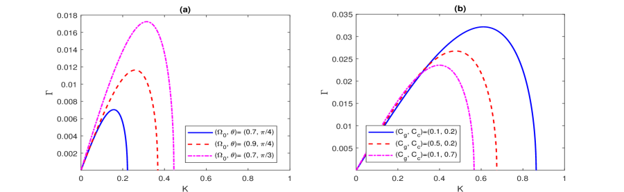
Figure 6: The instability growth rate $\Gamma$ vs. modulated wavenumber $K$ is plotted [Eq. (52)] for different values of parameters as mentioned in the legends. Here, $B_{0}=0.04$ and other parameters remain unchanged as in Fig. 2.

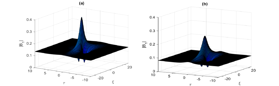
Figure 7: The three-dimensional first-order rogue wave profiles $|B_{1}|$ are displayed for $\Omega_{0}=0.7$ and $\Omega_{0}=0.9$ in the subplots (a) and (b), respectively. Here, $(C_{g},C_{c},\theta)=(0.1,0.7,\pi/3)$ and all other parameters remain unchanged as in Fig. 2.

Analytic Solution

Using the stationary wave frame $\chi=-(\xi-v\tau)$ moving with speed $v$ and integrating over the variable $\chi$, we obtain,

$$R\frac{d^{2}B}{d\chi^{2}}+S\frac{dB}{d\chi}+\frac{Q}{2}B^{2}-vB=0,$$ (32)

where we use the boundary conditions $B,\frac{dB}{d\chi},\frac{d^{2}B}{d\chi^{2}}\rightarrow 0$ as $\chi\rightarrow\pm\infty$. Following the method, we obtain a travelling wave solution of (21) as,

$$B(\chi)=a_{0}+a_{1}G(\chi)+a_{2}G^{2}(\chi),$$ (33)

where $G(\chi)=\sigma/2\left\{1+\tanh{[(\sigma/2)\chi]}\right\}$ is the solution of the Bernoulli’s equation,

$$\frac{dG(\chi)}{d\chi}=\sigma G(\chi)-G^{2}(\chi).$$ (34)

and the unknown constants $a_{i}$ ($i=0,1,2$) and $\sigma$ are to be calculated later. Differentiating Eq. (33) up to second order with respect to $\chi$, we obtain,

$$\frac{dB}{d\chi}=(a_{1}+2a_{2}G)(\sigma G-G^{2})$$ (35)

and

$$\frac{d^{2}B}{d\chi^{2}}=[a_{1}(\sigma-2G)+2a_{2}(2\sigma G-3G^{2})](\sigma G-G^{2}).$$ (36)

Plugging the expressions (33), (35) and (36) into (32) and collecting various terms of the same degree of $G$, we get,

$$a_{0}=2\frac{v}{Q},a_{1}=0,a_{2}=-12\frac{R}{Q},\sigma=-\frac{S}{5R}$$ (37)

and the speed of the moving frame $v=\frac{6D^{2}}{25R}$. Therefore, the localized solution of the KdVB equation (21) is written as follows,

$$B=\frac{3D^{2}}{25QR}\left[\mathrm{sech}\,^{2}{(\frac{S}{10R}\chi)}+2\left\{1+\tanh{(\frac{S}{10R}\chi)}\right\}\right],$$ (38)

which describes a composite form of solitary and Burger shock structure. In other words, the solution (38) represents an admixture of $\mathrm{sech}\,^{2}$ and $\tanh$ type waveform. The graphical representations of such profiles have been displayed in Fig. 4 for distinct parametric values, as stated in the caption of the corresponding figure. The figures reveal that, due to the increments in the values of the parameters $\Omega_{0}$, $\theta$, $\eta_{0}$ and $\kappa_{0}$, the amplitude is shifted to higher values, while the width becomes narrower for the monotonic shock wave pulses. Thus, cosmic ray diffusivity and magnetic resistivity play a key role in determining the nature and magnitude of the shock pulse in a dissipative magneto-rotating plasma under the effect of Coriolis force. The effect of modified pressure by combining the cosmic ray pressure (relating parameter $C_{c}$) with thermal pressure (relating parameter $C_{g}$) has been observed from the subplot (a) of Fig. 4. It has been noticed that when $C_{c}$ is fixed, the amplitude is shifted to lower values and the width becomes wider for increasing values of $C_{g}$; however, the amplitude increases and the width becomes narrower for increasing values of $C_{c}$.

Numerical Solution

Now, we numerically solve the Eq. (21) to look into further potential structures and their characteristics. To do so, we present Eq. (21) in the following coupled differential equation as

$$\begin{split}&\frac{dB}{d\chi}=Z,\\ &\frac{dZ}{d\chi}=\frac{v}{R}B-\frac{Q}{2R}B^{2}-\frac{S}{R}Z,\end{split}$$ (39)

which admits two fixed points, $(0,0)$ and $(2v/Q,0)$. Next, we employ the fourth-order Runge-Kutta method to solve Eq. (21) to study the effects of different parameters involved in the model, and the results obtained are displayed in Fig. 5. Subplots (a) and (b) show the effects of $C_{g}$ and $C_{c}$ on the oscillatory shock structures. We observe that as $C_{g}$ increases, the strength and width of the oscillatory shock grow, whereas they become smaller and tend to damp faster as $C_{c}$ increases. Subplots (c) and (d) illustrate how the rotational frequency $\Omega_{0}$ with the angle of rotation $\theta$ affects the oscillatory shock profiles. It is found that the oscillatory shock wave strength and width become smaller and tend to damp faster with increasing values of $\Omega_{0}$ with a fixed angle of rotation. On the other hand, the amplitude and width increase as $\theta$ increases for a fixed angle of rotation. Subplots (e) and (f) indicate that due to small increments in cosmic ray diffusivity $\kappa_{0}$ and magnetic resistivity $\eta_{0}$, the strength and width of oscillatory shock structures become smaller and tend to damp faster. The physical significance behind this phenomenon is that when the dissipative effects dominate the system, the monotone shock profile is formed, otherwise, the behaviour remains oscillatory.

V MODULATIONAL INSTABILITY AND ROGUE WAVE SOLUTIONS

In this section, we are interested in studying the magnetosonic wavepackets’ modulation instability (MI) and the characteristics of rogue wave solutions. In the limit of low frequency (i.e., when the carrier wave frequency is much smaller than the plasma frequency), neglecting the effect of magnetic resistivity and cosmic ray diffusivity, we derive a nonlinear Schrödinger (NLS) equation from Eq. (21) that describes the weakly nonlinear evolution of the modulated wave packet’s envelope. To this end, we consider the solution of Eq. (21) in the form of a weakly modulated sinusoidal wave,

$$B=\sum_{n=1}^{\infty}\epsilon^{n}\sum_{l=-\infty}^{\infty}B_{l}^{(n)}(X,T)\exp\left[il\left(k\xi-\omega\tau\right)\right].$$ (40)

Here, $k$ and $\omega$ are carrier wave number and angular frequency, respectively. Further, we stretched the coordinates, $X$ and $T$ as

$$\begin{split}X&=\epsilon\left(\xi-v_{g}\tau\right),\\ T&=\epsilon^{2}\tau,\end{split}$$ (41)

where $v_{g}$ denotes the group velocity, which will be calculated later. All perturbed quantities are supposed to vary on the fast scales through the phase $(k\xi-\omega\tau)$ only, while the slow scales (X, T) enter the arguments of the $l$-th harmonic amplitude $B_{l}^{n}$. $B_{l}^{(n)}$ is kept equal to its complex conjugate $B_{l}^{(n)*}$ to ensure that $B$ remains real. The two partial differential operators $\partial/\partial\tau$ and $\partial/\partial\xi$ can be replace as follows,

$$\begin{split}\frac{\partial}{\partial\tau}&\rightarrow\frac{\partial}{\partial\tau}-\epsilon v_{g}\frac{\partial}{\partial X}+\epsilon^{2}\frac{\partial}{\partial T},\\ \frac{\partial}{\partial\xi}&\rightarrow\frac{\partial}{\partial\xi}+\epsilon\frac{\partial}{\partial X}.\end{split}$$ (42)

Substituting the expressions from (40)-(42), into the Eq. (21), we obtain,

$$\begin{split}-i\omega lB_{l}^{(n)}-v_{g}\frac{\partial}{\partial T}B_{l}^{(n-1)}+\frac{\partial}{\partial T}B_{l}^{(n-2)}+A\sum_{n=1}^{\infty}\epsilon^{n}\sum_{l=-\infty}^{+\infty}\left(ilkB_{l}^{(n)}{B}_{l-l^{\prime}}^{(n-n^{\prime})}+{B}_{l-l^{\prime}}^{(n-n^{\prime}-1)}\frac{\partial}{\partial X}B_{l}^{(n)}\right)\\ +B\left(-il^{3}k^{3}B_{l}^{(n)}-3l^{2}k^{2}\frac{\partial{B}_{l}^{(n-1)}}{\partial X}+3ilk\frac{\partial^{2}{B}_{l}^{(n-2)}}{\partial X^{2}}+\frac{\partial^{3}{B}_{l}^{(n-3)}}{\partial X^{3}}\right)=0.\end{split}$$ (43)

In Eq. (43), from the first order with the first harmonic (i.e. $n=1$, $l=1$), we obtain the linear dispersion relation,

$$\omega=-Rk^{3}.$$ (44)

From the second order with the first harmonic (i.e. $n=2$, $l=1$), we obtain the expression for group velocity as

$$v_{g}=3Rk^{2}=\frac{\partial\omega}{\partial k}.$$ (45)

Similarly, for $n=2$ and $l=2$, we obtain $B_{2}^{(2)}=\frac{A}{6Rk^{2}}B_{1}^{(1)^{2}}$ and for $n=3$, $l=0$, we get $B_{0}^{(2)}=-\frac{Q}{v_{g}}|B_{1}^{(1)}|^{2}$. Proceeding to the third order ($n=3$) with the first harmonic ($l=1$), we obtain an explicit compatibility condition leading to the NLS equation,

$$i\frac{\partial B}{\partial T}+\frac{1}{2}M\frac{\partial^{2}B}{\partial X^{2}}+N|B|^{2}B=0,$$ (46)

where $B_{1}^{(1)}$ is replaced by $B$ for simplicity. The dispersion and the nonlinear coefficients in Eq. (46) are given by

$$M=6Rk$$ (47)

and

$$N=\frac{Q^{2}}{6Rk},$$ (48)

respectively. Eq. (46) describes the nonlinear evolution of modulated magnetosonic wave packet envelopes, which can also be obtained directly by plugging the Eqs. (40) and (42) into Eqs. (6)-(12). In that case, the NLS represents an arbitrary frequency wave carrier with much more complicated expressions for $M$ and $N$. However, in principle, the arbitrary frequency NLS equation should bring down to the Eq. (46) in the limit of low-frequency wave ruderman2008dynamics . The study of such low-frequency waves and the modulation of sinusoidal waves, which describe various physical phenomena in plasma, is quite natural.

To study the MI, we consider a small perturbation $\delta B$ such that $B=B_{0}+\delta B\exp{i\Delta B}$. $B_{0}$ is the amplitude of the carrier wave such that $|B_{0}|\gg|\Delta B|$, $\Delta$ being the nonlinear frequency shift. Using the expansion of $B$ in Eq. (46), we obtain,

$$\Delta=-Q|B_{0}|^{2}$$ (49)

and

$$i\frac{\partial B}{\partial T}+\frac{1}{2}M\frac{\partial^{2}B}{\partial X^{2}}+N|B_{0}|^{2}(\delta B+\delta B^{*})=0,$$ (50)

where $\delta B^{*}$ is the complex conjugate of $\delta B$. Assuming the amplitude perturbation varies as $\exp{(iKX-i\tilde{\Omega}T)}$, we derive the nonlinear dispersion relation as follows,

$$\tilde{\Omega}^{2}=M^{2}K^{2}(K^{2}-\frac{2B_{0}N}{M}).$$ (51)

Here, $K$ and $\tilde{\Omega}$ are modulated wave number and frequency, respectively. Based on the nonlinear analysis of the envelope dynamics, it is assumed that there are two kinds of envelope solitons, bright (unstable) and dark (stable). If $MN<0$, Eq. (51) possesses real solutions in terms of $\tilde{\Omega}$ for all real values of $K$, consequently, the magnetosonic waves become dark (stable) envelope solitons in this region. However, in our case where $MN>0$, the region carries bright (unstable) envelope solitons in the presence of small external perturbation. In this region, there exists a critical modulated wave number $K_{c}=\sqrt{2N|B_{0}|^{2}/M}$ below which $\tilde{\Omega}$ becomes imaginary, and MI takes place. For $MN>0$ and $K<K_{c}$, the growth rate of MI is specified as,

$$\Gamma=|M|K^{2}\sqrt{\frac{K_{c}^{2}}{K^{2}}-1}.$$ (52)

The maximum growth rate is $\Gamma_{max}=N|B_{0}|^{2}$ at $K=K_{c}/\sqrt{2}$. The growth rate of instability depends on the coefficients $M$ and $N$ (which are further influenced by various plasma parameters), any changes in the plasma parameters certainly change the growth rate of instability. The coefficients $M$ and $N$ are modified due to the inclusion of cosmic ray pressure, which affects the growth of the instability. The graphs of the growth rate $\Gamma$ have been plotted against the modulated wave number $K$ in Fig. 6 for different values of rotational frequency $\Omega_{0}$, angle of rotation $\theta$ (see subplot (a)), the parameter associated with thermal pressure $C_{g}$ and cosmic ray pressure $C_{c}$ (see subplot (b)), respectively. We note that $\Gamma$ increases with the increasing value of $\Omega_{0}$ and $\theta$, however, it decreases as the values of $C_{g}$ and $C_{c}$ increase. It has been noticed that including cosmic ray pressure in the present model reduces the instability growth. Furthermore, the plots in Fig. 6 show that the growth rate increases with increasing modulated wave number $K$ until it reaches a critical growth rate (say, $\Gamma_{c}$), which varies for different plasma parameters. After reaching the critical valued growth rate, it intensely decreases for further higher values of $K$. In particular, one can find $\Gamma_{c}=0.017$ at $K=0.3$ in the subplot (a) of Fig. 6 for $k=0.4$ and $\theta=\pi/3$.

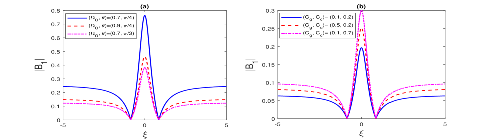
Figure 8: The first-order rogue wave pulses $|B_{1}|$ vs. $\xi$ [Eq. (53)] are plotted for different values of parameters as mentioned in the legends. Here, $K=0.4$ and all other parameters remain unchanged as in Fig. 2.

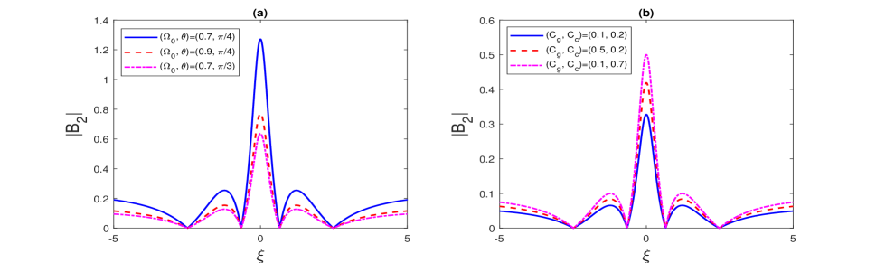
Figure 9: The second-order rogue wave pulses $|B_{2}|$ vs. $\xi$ (Eq. (54)) are plotted for different values of parameters as mentioned in the legends. Here, $K=0.4$ and all other parameters remain unchanged as in Fig. 2.

V.1 Rogue Wave solutions

The MI of the magnetosonic wavepackets leads to the generation of freak waves. Generations of such waves, in the region $MN>0$, are noticed to appear instantaneously and depart without any track down. Subsequently, the NLS Eq. (46) admits rational solutions localized in both space and time variables kharif2008rogue ; moslem2011dust as follows,

$$B_{1}(\xi,\tau)=\sqrt{M/N}\left[\frac{4(1+2iM\tau)}{1+4\xi^{2}+4M^{2}\tau^{2}}-1\right]\exp(iM\tau).$$ (53)

The first-order rational rogue solution (53) reveals that a significant amount of magnetosonic wave energy is concentrated in a relatively small area in space. Typically, rogue waves are the envelopes of carrier waves that have wavelengths smaller than those of the central region of the envelope. These waves have the unusual feature of not being periodic in both space and time. Combinations of multiple first-order rogue waves by nonlinear superpositions lead to higher-order rogue wave solutions having more complicated nonlinear forms and higher amplitude. The amplitude of such waves is generally four to five times the amplitude of the background wave. The existence of second-order rogue waves was experimentally observed by Chabchoub et al. chabchoub2012super in surface water gravity waves. The exact second-order rogue wave solution of the NSL equation (46) is given by akhmediev2009rogue ,

$$B_{2}(\xi,\tau)=\sqrt{M/N}\left(1+\frac{M_{2}+iN_{2}}{O_{2}}\right)\exp(iM\tau),$$ (54)

where

$$M_{2}=\frac{3}{8}-\frac{1}{2}\xi^{4}-\frac{3}{2}\xi^{2}-6(P\xi\tau)^{2}-10(P\tau)^{4}-9(P\tau)^{2},$$

$$N_{2}=-P\tau\left[-\frac{15}{4}+\xi^{4}-3\xi^{2}+4(P\xi\tau)^{2}+4(P\tau)^{4}+2(P\tau)^{2}\right],$$

$$O_{2}=\frac{3}{32}+\frac{1}{12}\xi^{6}+\frac{1}{8}\xi^{4}+\frac{1}{2}\xi^{4}(P\tau)^{2}+\frac{9}{16}\xi^{2}+\xi^{2}(P\tau)^{4}$$

$$-\frac{3}{2}(P\xi\tau)^{2}+\frac{2}{3}(P\tau)^{6}+\frac{9}{2}(P\tau)^{4}+\frac{33}{8}(P\tau)^{2}.$$

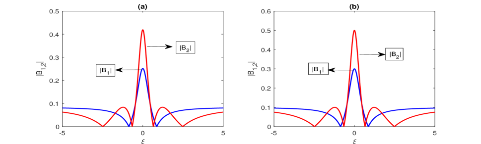
Figure 10: A comparison between first- and second-order rogue wave pulses $|B_{1}|,|B_{2}|$ is displayed against $\xi$. Here, $(C_{g},C_{c},\Omega_{0},\theta)=(0.5,0.2,0.9,\pi/3)$ and $(C_{g},C_{c},\Omega_{0},\theta)=(0.1,0.7,0.9,\pi/3)$ in subplots (a) and (b), respectively. All other parameters remain unchanged as in Fig. 2.

To gain some insight, we analyse the effects of the parameters $C_{g}$ and $C_{c}$ related to thermal and cosmic ray pressures, respectively, as well as the impact of the Coriolis force due to the rotation of the cosmic fluids with the angular frequency ($\Omega_{0}$) and the angle of rotation ($\theta$), on both the first- and second-order rogue wave solutions (53) and (54). Initially, the typical first-order rogue wave profiles $|B_{1}|$ are plotted against $\xi$ and $\tau$ for two different values of $\Omega_{0}$ in Fig. 7, keeping all other parameters fixed as mentioned in the figure caption. It has been observed that the amplitude and width of the rogue wave profile are reduced due to the enhancement of rotational frequency. The observation is quite natural, as the pulse can not gain energy from the background wave. To provide more specific details on the effects of the essential parameters on the evaluation of rogue waves, we plot the first-order rogue wave profiles $|B_{1}|$ against $\xi$ at an instant $\tau=0$ for different values of $\Omega_{0}$, $\theta$ (subplots (a) in Fig. 8) and $C_{g}$, $C_{c}$ (subplots (b) of Fig. 8). The figures illustrate that as the values of the parameters $\Omega_{0}$ and $\theta$ increase both the amplitude and width decrease, i.e., an increase in $\Omega_{0}$ and/or $\theta$ leads to the contraction of the rogue wave pulse. On the other hand, we notice that the inclusion of cosmic ray pressure with the thermal pressure significantly enlarges the rogue wave pulses. Subplot (b) in Fig. 8 depicts that both the amplitude and width increase with the increasing value of $C_{g}$ and $C_{c}$ related to the thermal pressure and cosmic ray pressure, respectively. These observations in Fig. 8) are found to be similar for the second-order solution $|B_{2}|$ versus $\xi$ in $\tau=0$ as displayed in Fig. 9. However, the second-order pulses’ amplitude is higher than that of first-order rogue wave pulses. The reduction (enhancement) of the amplitude and width of the rogue wave profiles, for both the first- and second-order solutions, signifies that the nonlinearity of the system diminishes (increases) due to the increase in the values of $\Omega_{0}$ and/or $\theta$ ($C_{g}$ and/or $C_{c}$ ). Hence, the Coriolis force due to the rotation of the cosmic fluids, and the modified pressure due to the inclusion of cosmic ray pressure with thermal pressure exhibit stabilizing behaviour on first- and second-order rogue wave solutions.

A comparison between the first- and second-order rogue wave solutions has been presented for different values of $\Omega_{0}$ and $\theta$ in Fig. 10. The figure illustrates that the second-order correction of the rogue wave solution leads to an enhancement of the amplitude and width of the wave pulses. It has been reported that the second-order rogue waves absorb more energy from the surrounding waves than the first-order rogue waves do, making them spikier than the first-order.

VI CONCLUSIONS

To conclude, we have investigated the evaluation of linear and nonlinear magnetosonic waves in the interstellar medium of spiral galaxies, which are the combination of thermal and cosmic fluid, taking into account the magneto-rotational effects of the fluid. The typical consistent parameters adopted in our numerical assessment are relevant in such fluid mediums of spiral galaxies gliddon1966gravitational ; turi2022magnetohydrodynamic . The cosmic fluid is found to have a reasonable contribution in modifying the thermal pressure in terms of the system’s total pressure. Consequently, the dispersion properties, nonlinear wave evaluation, and modulation instabilities are modified. The effects of the parameters $C_{g}$ and $C_{c}$, related to the thermal and cosmic ray pressure, respectively, have been demonstrated. The Coriolis force due to the rotation of the plasma is found to have significant refinement in the wave propagation as the rotation frequency ($\Omega_{0}$) and rotation angle ($\theta$) vary. Further, cosmic ray diffusivity ($\kappa$) and magnetic resistivity ($\eta$) play a crucial role in evaluating shock waves. The significant results obtained are summarized as follows:

• The linear analysis reveals that the dispersion relation (III) remains the same as obtained in Turi and Misraturi2022magnetohydrodynamic in the absence of both cosmic ray diffusivity ($\kappa$) and magnetic resistivity ($\eta$). The waves become unstable due to the increase in the values of the parameters $\eta$ and $\kappa$. However, interestingly, the damping caused by cosmic ray diffusivity and magnetic resistivity becomes negligible as one increases the rotating frequency. Wave damping is reduced by increasing the effects of the rotational effect in the system. The damping is also modified due to the presence of cosmic fluid in the system by accelerating the damping rate $|\gamma|$.

• To perform nonlinear analysis, we first derived a KdVB equation by employing the reductive perturbation technique. In solving the KdVB equation, several nonlinear wave shapes have been evaluated, analytically, and numerically. The results indicate that the parameters of cosmic ray diffusivity ($\kappa_{0}$) and magnetic resistivity ($\eta_{0}$) are responsible for the formation of shock structures in the current model. When the effects of $\kappa_{0}$ and $\eta_{0}$ grow considerably, the dispersion effect becomes negligible compared to dissipation, and the monotonic shocks become stationary. Additionally, it has been noticed that the numerical solutions lead to oscillatory shock wave profiles, and growing values of $\kappa_{0}$, $\eta_{0}$ and rotation coefficients produce damped oscillatory waves with reduced amplitude. The KdVB equation becomes the KdV equation without the presence of $\eta_{0}$ and $\kappa_{0}$, consequently, the solitary wave evaluation has been reported.

• To characterize the weakly nonlinear development of the envelope of a modulated wave packet in the low-frequency limit, we derive a nonlinear Schrödinger (NLS) equation from Eq. (21). It has been noticed that incorporating cosmic ray pressure in the present model reduces MI growth. As the modulated wave number $K$ increases, the growth rate rises until it hits a critical growth rate $\Gamma_{c}$, which varies depending on the plasma properties. It sharply declines for even higher values of $K$ after hitting the critical value growth rate. Furthermore, the present model supports the propagation of magnetosonic rogue waves. It is observed that the Coriolis force reduces the system’s nonlinearity, resulting in a shorter rogue wave amplitude, however, the inclusion of cosmic ray pressure with the thermal pressure significantly enlarges the rogue wave pulses.

Our investigation is based on typical plasma parameters: $B_{0}\sim 1$ nT, $\rho_{0}\sim 10^{-21}$ Kg/m³, $P_{g0}\sim 10^{-13}$ N/m², $P_{c0}\sim 10^{-13}$N/m², $\eta\sim 10^{-1}V_{A}^{2}/\omega_{ci}$ and $\kappa\sim 10^{-2}V_{A}^{2}/\omega_{ci}$ which are relevant to the spiral galaxies. gliddon1966gravitational ; turi2022magnetohydrodynamic Thus, we believe the present study could be useful for understanding the magnetosonic wave propagation in the interstellar medium of spiral galaxies, where cosmic rays play an important role.

Data availability statement

Data sharing is not applicable to this article as no new data were created or analyzed in this study.

References

- (1) T. Kuwabara, C.-M. Ko, Dynamics of the parker–jeans instability of gaseous disks including the effect of cosmic rays, The Astrophysical Journal 899 (1) (2020) 72.
- (2) E. Parker, Galactic effects of the cosmic-ray gas, Space Science Reviews 9 (5) (1969) 651–712.
- (3) M. Padovani, A. V. Ivlev, D. Galli, S. S. Offner, N. Indriolo, D. Rodgers-Lee, A. Marcowith, P. Girichidis, A. M. Bykov, J. D. Kruijssen, Impact of low-energy cosmic rays on star formation, Space Science Reviews 216 (2) (2020) 29.
- (4) J. Kalvāns, Temperature spectra of interstellar dust grains heated by cosmic rays. i. translucent clouds, The Astrophysical Journal Supplement Series 224 (2) (2016) 42.
- (5) F. Yusef-Zadeh, M. Wardle, S. Roy, Cosmic-ray heating of molecular gas in the nuclear disk: Low star formation efficiency, The Astrophysical Journal 665 (2) (2007) L123.
- (6) B. A. Gaches, S. S. Offner, T. G. Bisbas, The astrochemical impact of cosmic rays in protoclusters. i. molecular cloud chemistry, The Astrophysical Journal 878 (2) (2019) 105.
- (7) M. Padovani, D. Galli, Effects of magnetic fields on the cosmic-ray ionization of molecular cloud cores, Astronomy & Astrophysics 530 (2011) A109.
- (8) N. Indriolo, B. D. Fields, B. J. McCall, The implications of a high cosmic-ray ionization rate in diffuse interstellar clouds, The Astrophysical Journal 694 (1) (2009) 257.
- (9) C. Goertz, Dusty plasmas in the solar system, Reviews of Geophysics 27 (2) (1989) 271–292.
- (10) O. Havnes, F. Melandsø, C. La Hoz, T. Aslaksen, T. Hartquist, Charged dust in the earth’s mesopause; effects on radar backscatter, Physica Scripta 45 (5) (1992) 535.
- (11) M. Horanyi, D. Mendis, The effects of electrostatic charging on the dust distribution at halley’s comet, Astrophysical Journal, Part 1 (ISSN 0004-637X), vol. 307, Aug. 15, 1986, p. 800-807. 307 (1986) 800–807.
- (12) A.-M. Wazwaz, Abundant solutions of various physical features for the (2+ 1)-dimensional modified kdv-calogero–bogoyavlenskii–schiff equation, Nonlinear Dynamics 89 (3) (2017) 1727–1732.
- (13) S. Chen, Y. Zhou, F. Baronio, D. Mihalache, et al., Special types of elastic resonant soliton solutions of the kadomtsev–petviashvili ii equation, Rom. Rep. Phys 70 (102) (2018) 16.
- (14) N. El-Bedwehy, On the generation of cnoidal waves in ion beam-dusty plasma containing superthermal electrons and ions, Physics of Plasmas 23 (7) (2016).
- (15) D. Mihalache, Multidimensional localized structures in optical and matter-wave media: a topical survey of recent literature, Rom. Rep. Phys 69 (1) (2017) 403.
- (16) N. Akhmediev, A. Ankiewicz, M. Taki, Waves that appear from nowhere and disappear without a trace, Physics Letters A 373 (6) (2009) 675–678.
- (17) P. Müller, C. Garrett, A. Osborne, Rogue waves, Oceanography 18 (3) (2005) 66.
- (18) K. Sharma, J. Turi, R. Ali, U. Deka, Modulation instability of magnetosonic waves in semiconducting quantum plasma considering fermi degenerate pressure, exchange correlation potential, and bohm potential, Physics of Fluids 36 (7) (2024).
- (19) S. Chen, D. Mihalache, Vector rogue waves in the manakov system: diversity and compossibility, Journal of Physics A: Mathematical and Theoretical 48 (21) (2015) 215202.
- (20) C. Kharif, E. Pelinovsky, A. Slunyaev, Rogue waves in the ocean, Springer Science & Business Media, 2008.
- (21) D. R. Solli, C. Ropers, P. Koonath, B. Jalali, Optical rogue waves, nature 450 (7172) (2007) 1054–1057.
- (22) Y. V. Bludov, V. Konotop, N. Akhmediev, Matter rogue waves, Physical Review A 80 (3) (2009) 033610.
- (23) L. Stenflo, M. Marklund, Rogue waves in the atmosphere, Journal of Plasma Physics 76 (3-4) (2010) 293–295.
- (24) R. Sabry, W. Moslem, P. Shukla, Freak waves in white dwarfs and magnetars, Physics of Plasmas 19 (12) (2012).
- (25) Z. Rahim, M. Adnan, A. Qamar, Magnetosonic shock waves in magnetized quantum plasma with the evolution of spin-up and spin-down electrons, Physical Review E 100 (5) (2019) 053206.
- (26) Y. A. Hager, M. A. Khaled, M. A. Shukri, Magnetosonic waves propagation in a magnetorotating quantum plasma, Physical Review E 107 (5) (2023) 055202.
- (27) S. El-Labany, W. Moslem, N. El-Bedwehy, R. Sabry, H. Abd El-Razek, Rogue wave in titan’s atmosphere, Astrophysics and Space Science 338 (2012) 3–8.
- (28) W. Moslem, P. Shukla, B. Eliasson, Surface plasma rogue waves, Europhysics Letters 96 (2) (2011) 25002.
- (29) M. Akbari-Moghanjoughi, Electrostatic rogue-waves in relativistically degenerate plasmas, Physics of Plasmas 21 (10) (2014).
- (30) J. Turi, A. Misra, Magnetohydrodynamic instabilities in a self-gravitating rotating cosmic plasma, Physica Scripta 97 (12) (2022) 125603.
- (31) P. Boro, R. P. Prajapati, Cosmic ray-driven magnetohydrodynamic waves in magnetized self-gravitating dusty molecular clouds, Monthly Notices of the Royal Astronomical Society 522 (2) (2023) 1752–1762.
- (32) A. Bonanno, V. Urpin, Generation of magnetosonic waves and formation of structures in galaxies, Monthly Notices of the Royal Astronomical Society 388 (4) (2008) 1679–1685.
- (33) G. Zank, G. Webb, Weakly multi-dimensional cosmic-ray-modified mhd shocks, Journal of plasma physics 44 (1) (1990) 91–101.
- (34) J. Gliddon, Gravitational instability of anisotropic plasma, Astrophysical Journal, vol. 145, p. 583 145 (1966) 583.
- (35) A. Abdikian, M. Eghbali, A. Misra, Drift ion-acoustic waves in a nonuniform rotating magnetoplasma with two-temperature superthermal electrons, Physica Scripta 97 (4) (2022) 045603.
- (36) Y. Nakamura, H. Bailung, P. Shukla, Observation of ion-acoustic shocks in a dusty plasma, Physical review letters 83 (8) (1999) 1602.
- (37) Y. Nakamura, A. Sarma, Observation of ion-acoustic solitary waves in a dusty plasma, Physics of Plasmas 8 (9) (2001) 3921–3926.
- (38) R. Hirota, Exact solution of the korteweg—de vries equation for multiple collisions of solitons, Physical Review Letters 27 (18) (1971) 1192.
- (39) P. G. Drazin, R. S. Johnson, Solitons: an introduction, Vol. 2, Cambridge university press, 1989.
- (40) M. M. Hossen, L. Nahar, M. Alam, S. Sultana, A. Mamun, Electrostatic shock waves in a nonthermal dusty plasma with oppositely charged dust, High Energy Density Physics 24 (2017) 9–14.
- (41) M. S. Ruderman, T. Talipova, E. Pelinovsky, Dynamics of modulationally unstable ion-acoustic wavepackets in plasmas with negative ions, Journal of plasma physics 74 (5) (2008) 639–656.
- (42) W. Moslem, R. Sabry, S. El-Labany, a. K. Shukla, Dust-acoustic rogue waves in a nonextensive plasma, Physical Review E 84 (6) (2011) 066402.
- (43) A. Chabchoub, N. Hoffmann, M. Onorato, N. Akhmediev, Super rogue waves: observation of a higher-order breather in water waves, Physical Review X 2 (1) (2012) 011015.
- (44) N. Akhmediev, A. Ankiewicz, J. M. Soto-Crespo, Rogue waves and rational solutions of the nonlinear schrödinger equation, Physical Review E 80 (2) (2009) 026601.