Max-Normalized Radon Cumulative Distribution Transform for Limited Data Classification

Abstract

The Radon cumulative distribution transform (R-CDT) exploits one-dimensional Wasserstein transport and the Radon transform to represent prominent features in images. It is closely related to the sliced Wasserstein distance and facilitates classification tasks, especially in the small data regime, like the recognition of watermarks in filigranology. Here, a typical issue is that the given data may be subject to affine transformations caused by the measuring process. The aim of this paper is to make the R-CDT and the related sliced Wasserstein distance invariant under affine transformations. For this, we propose a two-step normalization of the R-CDT and prove that our novel transform allows linear separation of affinely transformed image classes. The theoretical results are supported by numerical experiments showing a significant increase of the classification accuracy compared to the original R-CDT.

.

1 Introduction

Automated pattern recognition and classification play a central role in numerous applications and disciplines, be it in medical imaging, biometrics, or document analysis. Nowadays, in the big data regime, end-to-end deep neural networks provide the latest state of the art. In the small data regime, however, hand-crafted feature extractors and classifiers still stand their ground. Ideally, the feature extractor is designed to transform different classes to linear separable subsets. This may, for instance, be achieved by the so-called Radon cumulative distribution transform (R-CDT) introduced in [7], which is based on one-dimensional optimal transport maps that are generalized to two-dimensional data by applying the Radon transform, known from tomography [13, 10]. This approach shows great potential in many applications [8, 5, 14] and is closely related to the sliced Wasserstein distance [3, 15]. A similar approach for data on the sphere is studied in [11, 12], for multi-dimensional optimal transport maps in [9], and for optimal Gromov–Wasserstein transport maps in [2].

A central inspiration for this paper is the application of pattern recognition techniques in filigranology—the study of watermarks. These play a central role in dating historical manuscripts as well as identifying scribes and papermills. For automatic classification, the main issue is the enormous number of classes with only few members per class, see WZIS. An end-to-end processing pipeline for thermograms of watermarks including an R-CDT-based classification is proposed in [6], where the authors report classification invariance with respect to translation and dilation of the watermark. Other affine transformations caused, e.g., by unstandardized recording methods are, however, not included yet.

Contribution.

The aim of this paper is to incorporate invariance with respect to affine transformations into the R-CDT, this is, to make the sliced Wasserstein distance unaware of these transforms. In difference to [14], where the dataset is augmented to encode invariances, we propose a two-step normalization of the R-CDT for probability measures on $\mathbb{R}^{2}$. To this end, we first generalize the classical Radon transform to measures in § 2 and, thereon, introduce the novel max-normalized R-CDT (_mNR-CDT) in § 3. Our main theoretical contribution is Theorem 3.1 ensuring the linear separability of affinely transformed measure classes by _mNR-CDT. The theoretical findings are supported by proof-of-concept experiments in § 4 showing a significant improvement of the classification accuracy by the proposed normalization, especially in the small data regime.

2 Radon Transform

The main idea behind the classical Radon transform [10] is to integrate a given bivariate function along all parallel lines pointing in a certain direction. This integral transform can also be interpreted as projection of the given function onto the line with orthogonal orientation. In the following, we briefly review the classical Radon transform for functions and generalize the concept to measures. Finally, we study the effect of affine transformations on the Radon transform, which is crucial to solve the classification task at hand.

2.1 Radon Transform of Functions

Depending on ${\bm{\theta}}\in\mathbb{S}_{1}\coloneqq\{\mathbf{x}\in\mathbb{R}^{2}\mid\lVert\mathbf{x}\rVert=1\}$, we introduce the slicing operator $S_{\bm{\theta}}\colon\mathbb{R}^{2}\to\mathbb{R}$ by

$$S_{\bm{\theta}}(\mathbf{x})\coloneqq\langle\mathbf{x},{\bm{\theta}}\rangle,\quad\mathbf{x}\in\mathbb{R}^{2}.$$

Its preimages $S_{\bm{\theta}}^{-1}(t)$, $t\in\mathbb{R}$, are the lines $\ell_{t,{\bm{\theta}}}$ in direction ${\bm{\theta}}^{\perp}\coloneqq(\theta_{2},-\theta_{1})^{\top}\in\mathbb{S}_{1}$ with distance $t$ to the origin. More precisely, we have

$$\ell_{t,{\bm{\theta}}}\coloneqq S_{\bm{\theta}}^{-1}(t)=\{t{\bm{\theta}}+\tau{\bm{\theta}}^{\perp}\mid\tau\in\mathbb{R}\}\subset\mathbb{R}^{2}.$$

Using the bijection $\varphi_{\bm{\theta}}\colon\mathbb{R}^{2}\to\mathbb{R}^{2}$ defined as $\varphi_{\bm{\theta}}(t,\tau)\coloneqq t\,{\bm{\theta}}+\tau\,{\bm{\theta}}^{\perp}$, whose inverse is given by $\varphi_{\bm{\theta}}(\mathbf{x})^{-1}=(\langle\mathbf{x},{\bm{\theta}}\rangle,\langle\mathbf{x},{\bm{\theta}}^{\perp}\rangle)$, we parameterize $\ell_{t,{\bm{\theta}}}$ via $\tau\mapsto\varphi_{\bm{\theta}}(t,\tau)$.

For $f\in L^{1}(\mathbb{R}^{2})$, we define its Radon transform $\mathcal{R}[f]\colon\mathbb{R}\times\mathbb{S}_{1}\to\mathbb{R}$ as the line integral

$$\mathcal{R}[f](t,{\bm{\theta}})\coloneqq\int_{\ell_{t,{\bm{\theta}}}}f(s)\mathop{}\!\mathrm{d}s,\quad(t,{\bm{\theta}})\in\mathbb{R}\times\mathbb{S}_{1},$$

where $\mathop{}\!\mathrm{d}s$ denotes the arc length element of $\ell_{t,{\bm{\theta}}}$. This defines the Radon operator $\mathcal{R}\colon L^{1}(\mathbb{R}^{2})\to L^{1}(\mathbb{R}\times\mathbb{S}_{1})$. For fixed ${\bm{\theta}}\in\mathbb{S}_{1}$, we set $\mathcal{R}_{\bm{\theta}}\coloneqq\mathcal{R}(\cdot,{\bm{\theta}})$, which is referred to as the restricted Radon operator $\mathcal{R}_{\bm{\theta}}\colon L^{1}(\mathbb{R}^{2})\to L^{1}(\mathbb{R})$. The action of the Radon operator is illustrated in Figure 1.

Figure 1: Illustration of the bivariate Radon transform with distance $t\in\mathbb{R}$ and normal direction ${\bm{\theta}}\in\mathbb{S}_{1}$. The given function is integrated along the lines $\ell_{t,{\bm{\theta}}}$.

The Radon transform is also well-defined for all $f\in L^{p}(\mathbb{R}^{2})$ with $p\geq 1$ and $\operatorname{supp}(f)\subseteq\mathbb{B}_{2}\coloneqq\{\mathbf{x}\in\mathbb{R}^{2}\mid\lVert\mathbf{x}\rVert\leq 1\}$, in which case $\mathcal{R}[f]\in L^{p}(\mathbb{R}\times\mathbb{S}_{1})$ with $\operatorname{supp}(\mathcal{R}[f])\subseteq\mathbb{I}\times\mathbb{S}_{1}$, where $\mathbb{I}\coloneqq[-1,1]$.

According to [10], the adjoint $\mathcal{R}^{*}\colon L^{\infty}(\mathbb{R}\times\mathbb{S}_{1})\to L^{\infty}(\mathbb{R}^{2})$ of the Radon operator $\mathcal{R}\colon L^{1}(\mathbb{R}^{2})\to L^{1}(\mathbb{R}\times\mathbb{S}_{1})$ is given by the back projection

$$\mathcal{R}^{*}[g](\mathbf{x})\coloneqq\int_{\mathbb{S}_{1}}g(S_{\bm{\theta}}(\mathbf{x}),{\bm{\theta}})\mathop{}\!\mathrm{d}\sigma_{\mathbb{S}_{1}}({\bm{\theta}}),\quad\mathbf{x}\in\mathbb{R}^{2},$$

where $\sigma_{\mathbb{S}_{1}}$ denotes the surface measure on $\mathbb{S}_{1}$.

2.2 Radon Transform of Measures

The concept of the Radon transform is now translated to signed, regular, finite measures $\mu\in\mathcal{M}(\mathbb{R}^{2})$. For a fixed direction ${\bm{\theta}}\in\mathbb{S}_{1}$, we generalize the restricted Radon transform $\mathcal{R}_{\bm{\theta}}$ to measures by setting

$$\mathcal{R}_{\bm{\theta}}\colon\mathcal{M}(\mathbb{R}^{2})\to\mathcal{M}(\mathbb{R}),\quad\mu\mapsto(S_{\bm{\theta}})_{\#}\mu=\mu\circ S_{\bm{\theta}}^{-1},$$

which corresponds to the integration along $\ell_{t,{\bm{\theta}}}$. Note that $\mathcal{R}_{\bm{\theta}}[\mu](\mathbb{R})=\mu(\mathbb{R}^{2})$ for all ${\bm{\theta}}\in\mathbb{S}_{1}$ and, thus, the mass of $\mu$ is preserved by $\mathcal{R}_{\bm{\theta}}$. In measure theory, $\mathcal{R}_{\bm{\theta}}$ can be considered as a disintegration family. Heuristically, we may generalize the Radon transform by integrating $\mathcal{R}_{\bm{\theta}}$ along ${\bm{\theta}}\in\mathbb{S}_{1}$. Therefore, we define the Radon transform $\mathcal{R}\colon\mathcal{M}(\mathbb{R}^{2})\to\mathcal{M}(\mathbb{R}\times\mathbb{S}_{1})$ via

$$\mathcal{R}[\mu]\coloneqq\mathcal{I}_{\#}[\mu\times u_{\mathbb{S}_{1}}]$$ (1)

with $\mathcal{I}(\mathbf{x},{\bm{\theta}})\coloneqq(S_{\bm{\theta}}(\mathbf{x}),{\bm{\theta}})$ for $(\mathbf{x},{\bm{\theta}})\in\mathbb{R}^{2}\times\mathbb{S}_{1}$. Here $\mu\times u_{\mathbb{S}_{1}}$ denotes the product measure between the given $\mu$ and the uniform measure $u_{\mathbb{S}_{1}}\coloneqq\sigma_{\mathbb{S}_{1}}/2\pi$ on $\mathbb{S}_{1}$.

Proposition 1

Let $\mu\in\mathcal{M}(\mathbb{R}^{2})$. Then, $\mathcal{R}[\mu]$ can be disintegrated into the family $\mathcal{R}_{\bm{\theta}}[\mu]$ with respect to $u_{\mathbb{S}_{1}}$, i.e., for all continuous $g\in C_{0}(\mathbb{R}\times\mathbb{S}_{1})$ vanishing at infinity, we have

$$\langle\mathcal{R}[\mu],g\rangle=\int_{\mathbb{S}_{1}}\langle\mathcal{R}_{{\bm{\theta}}}[\mu],g(\cdot,{\bm{\theta}})\rangle\mathop{}\!\mathrm{d}u_{\mathbb{S}_{1}}({\bm{\theta}}).$$

Proof

By definition in (1), we obtain

$$\langle\mathcal{R}[\mu],g\rangle =\int_{\mathbb{R}\times\mathbb{S}_{1}}g(t,{\bm{\theta}})\mathop{}\!\mathrm{d}\mathcal{I}_{\#}[\mu\times u_{\mathbb{S}_{1}}](t,{\bm{\theta}})=\int_{\mathbb{S}_{1}}\int_{\mathbb{R}^{2}}g(S_{\bm{\theta}}(\mathbf{x}),{\bm{\theta}})\mathop{}\!\mathrm{d}\mu(\mathbf{x})\mathop{}\!\mathrm{d}u_{\mathbb{S}_{1}}({\bm{\theta}})$$

$$=\int_{\mathbb{S}_{1}}\int_{\mathbb{R}^{2}}g(t,{\bm{\theta}})\mathop{}\!\mathrm{d}[(S_{\bm{\theta}})_{\#}\mu](t)\mathop{}\!\mathrm{d}u_{\mathbb{S}_{1}}({\bm{\theta}})=\int_{\mathbb{S}_{1}}\langle\mathcal{R}_{{\bm{\theta}}}[\mu],g(\cdot,{\bm{\theta}})\rangle\mathop{}\!\mathrm{d}u_{\mathbb{S}_{1}}({\bm{\theta}})$$

using Fubini’s theorem. ∎

One can find the measure-valued Radon transform $\mathcal{R}\colon\mathcal{M}(\mathbb{R}^{2})\to\mathcal{M}(\mathbb{R}\times\mathbb{S}_{1})$ as the adjoint of the function-valued adjoint $\mathcal{R}^{*}\colon L^{\infty}(\mathbb{R}\times\mathbb{S}_{1})\to L^{\infty}(\mathbb{R}^{2})$, similar to the case of distributions with compact support, cf. [13].

Proposition 2

The Radon transform of $\mu\in\mathcal{M}(\mathbb{R}^{2})$ satisfies

$$\langle\mathcal{R}[\mu],g\rangle=\langle\mu,\mathcal{R}^{*}[g]\rangle\quad\forall\,g\in L^{\infty}(\mathbb{R}\times\mathbb{S}_{1}).$$

Proof

For all $\mu\in\mathcal{M}(\mathbb{R}^{2})$ and $g\in L^{\infty}(\mathbb{R}\times\mathbb{S}_{1})$, applying Fubini’s theorem gives

$$\langle\mathcal{R}[\mu],g\rangle=\int_{\mathbb{R}\times\mathbb{S}_{1}}g(t,{\bm{\theta}})\mathop{}\!\mathrm{d}\mathcal{I}_{\#}[\mu\times u_{\mathbb{S}_{1}}](t,{\bm{\theta}})=\int_{\mathbb{R}^{2}}\int_{\mathbb{S}_{1}}g(S_{\bm{\theta}}(\mathbf{x}),{\bm{\theta}})\mathop{}\!\mathrm{d}u_{\mathbb{S}_{1}}({\bm{\theta}})\mathop{}\!\mathrm{d}\mu(\mathbf{x}).$$ ∎

Note that, for $f\in L^{1}(\mathbb{R}^{2})$ and the Lebesgue measure $\lambda_{\mathbb{R}^{2}}$ on $\mathbb{R}^{2}$, the Radon transform satisfies

$$\mathcal{R}[f\,\lambda_{\mathbb{R}^{2}}]=\mathcal{R}[f]\,\sigma_{\mathbb{R}\times\mathbb{S}_{1}},$$

where $\sigma_{\mathbb{R}\times\mathbb{S}_{1}}$ denotes the surface measure on $\mathbb{R}\times\mathbb{S}_{1}$. In particular, the Radon transform of an absolutely continuous measure is again absolutely continuous.

2.3 Radon Transform of Affine Transformations

We now consider the Radon transform of an affinely transformed finite measure $\mu\in\mathcal{M}(\mathbb{R}^{2})$. To this end, let $\mathbf{A}\in\mathrm{GL}(2)$ and $\mathbf{y}\in\mathbb{R}^{2}$, this is, $\mathbf{A}$ is contained in the general linear group $\mathrm{GL}$ of regular matrices. We define $\mu_{\mathbf{A},\mathbf{y}}\in\mathcal{M}(\mathbb{R}^{2})$ via

$$\mu_{\mathbf{A},\mathbf{y}}\coloneqq(\mathbf{A}\cdot+\mathbf{y})_{\#}\mu=\mu\circ(\mathbf{A}^{-1}(\cdot-\mathbf{y})).$$ (2)

Proposition 3

For any ${\bm{\theta}}\in\mathbb{S}_{1}$, the restricted Radon transform satisfies

$$\mathcal{R}_{{\bm{\theta}}}[\mu_{\mathbf{A},\mathbf{y}}]=(\lVert\mathbf{A}^{\top}{\bm{\theta}}\rVert\cdot+\langle\mathbf{y},{\bm{\theta}}\rangle)_{\#}\mathcal{R}_{\frac{\mathbf{A}^{\top}{\bm{\theta}}}{\lVert\mathbf{A}^{\top}{\bm{\theta}}\rVert}}[\mu]=\mathcal{R}_{\frac{\mathbf{A}^{\top}{\bm{\theta}}}{\lVert\mathbf{A}^{\top}{\bm{\theta}}\rVert}}[\mu]\circ\Bigl{(}\tfrac{\cdot-\langle\mathbf{y},{\bm{\theta}}\rangle}{\lVert\mathbf{A}^{\top}{\bm{\theta}}\rVert}\Bigr{)}.$$

Proof

Direct calculations yield

$$\mathcal{R}_{{\bm{\theta}}}[\mu_{\mathbf{A},\mathbf{y}}] =(S_{\bm{\theta}})_{\#}[(\mathbf{A}\cdot+\mathbf{y})_{\#}\mu]=(\langle\mathbf{A}\cdot+\mathbf{y},{\bm{\theta}}\rangle)_{\#}\mu=(\langle\cdot,\mathbf{A}^{\top}{\bm{\theta}}\rangle+\langle\mathbf{y},{\bm{\theta}}\rangle)_{\#}\mu$$

$$=\bigl{(}\lVert\mathbf{A}^{\top}{\bm{\theta}}\rVert\bigl{\langle}\cdot,\tfrac{\mathbf{A}^{\top}{\bm{\theta}}}{\lVert\mathbf{A}^{\top}{\bm{\theta}}\rVert}\bigr{\rangle}+\langle\mathbf{y},{\bm{\theta}}\rangle\bigr{)}_{\#}\mu=(\lVert\mathbf{A}^{\top}{\bm{\theta}}\rVert\cdot+\langle\mathbf{y},{\bm{\theta}}\rangle)_{\#}\mathcal{R}_{\frac{\mathbf{A}^{\top}{\bm{\theta}}}{\lVert\mathbf{A}^{\top}{\bm{\theta}}\rVert}}[\mu],$$

and the proof is complete. ∎

Table 1: Summary of common transformations for $\mu\in\mathcal{M}(\mathbb{R}^{2})$ with $a,b>0$ and $c,\varphi\in\mathbb{R}$. The unit circle is parameterized by ${\bm{\theta}}(\vartheta)\coloneqq(\cos(\vartheta),\sin(\vartheta))^{\top}$. The Radon transform for the left half of $\mathbb{S}_{1}$ follows by symmetry.

transformation	$\mathbf{A}$	$\mathbf{y}$	$\mathcal{R}_{{\bm{\theta}}(\vartheta)}[\mu_{\mathbf{A},\mathbf{y}}]$, $\vartheta\in(-\tfrac{\pi}{2},\tfrac{\pi}{2})$
translation	$\mathbf{I}$	$\mathbb{R}^{2}$	$\mathcal{R}_{{\bm{\theta}}(\vartheta)}[\mu]\circ(\cdot-\langle\mathbf{y},{\bm{\theta}}(\vartheta)\rangle)$
rotation	$\bigl{(}\begin{smallmatrix}\cos(\varphi)&-\sin(\varphi)\\ \sin(\varphi)&\hphantom{-}\cos(\varphi)\end{smallmatrix}\bigr{)}$	$\mathbf{0}$	$\mathcal{R}_{{\bm{\theta}}(\vartheta-\varphi)}[\mu]$
reflection	$\bigl{(}\begin{smallmatrix}\cos(\varphi)&\hphantom{-}\sin(\varphi)\\ \sin(\varphi)&-\cos(\varphi)\end{smallmatrix}\bigr{)}$	$\mathbf{0}$	$\mathcal{R}_{{\bm{\theta}}(\varphi-\vartheta)}[\mu]$
anisotropic scaling	$\bigl{(}\begin{smallmatrix}a&0\\ 0&b\end{smallmatrix}\bigr{)}$	$\mathbf{0}$	$\mathcal{R}_{{\bm{\theta}}(\arctan(\frac{b}{a}\tan(\vartheta)))}[\mu]\circ([a^{2}\cos^{2}(\vartheta)+b^{2}\sin^{2}(\vartheta)]^{-1/2}\cdot)$
vertical shear	$\bigl{(}\begin{smallmatrix}1&0\\ c&1\end{smallmatrix}\bigr{)}$	$\mathbf{0}$	$\mathcal{R}_{{\bm{\theta}}(\arctan(c+\tan(\vartheta)))}[\mu]\circ([1+c^{2}\cos^{2}(\vartheta)+c\sin(2\vartheta)]^{-1/2}\cdot)$

The effect of common affine transformations on the Radon transform is given in Table 1. In order to describe the deformation with respect to ${\bm{\theta}}$, we over-parameterize the unit circle $\mathbb{S}_{1}$ via ${\bm{\theta}}(\vartheta)\coloneqq(\cos(\vartheta),\sin(\vartheta))^{\top}$, $\vartheta\in\mathbb{R}$. As by Proposition 3, an affine transformation essentially causes a transition and dilation of the transformed measure together with a non-affine remapping in ${\bm{\theta}}$.

3 Optimal Transport-Based Transforms

The aim of the following is to introduce an image distance that is unaware of affine transformations. Methodologically, we rely on the Radon cumulative distribution transform (R-CDT) introduced in [7], which allows to utilize the fast-to-compute, one-dimensional Wasserstein distance in the context of image processing due to a Radon-based slicing technique. As the R-CDT is not invariant under affine transformation by itself, we propose a two-step normalization scheme, which is essentially grounded on our observations regarding the Radon transform under affine transformations in § 2.3. Finally, we study the linear separability of affinely transformed image classes by our novel normalized R-CDT.

3.1 R-CDT for Measures

The R-CDT traces back to Kolouri et al. [7] and transforms smooth, bivariate density functions. In difference to [7], we introduce the concept for arbitrary probability measures, similar to [5]. In a first step, we consider probability measures $\mathcal{P}(\mathbb{R})\subset\mathcal{M}(\mathbb{R})$ defined on the real line. For $\mu\in\mathcal{P}(\mathbb{R})$, the cumulative distribution function $F_{\mu}\colon\mathbb{R}\to[0,1]$ is given by $F_{\mu}(t)\coloneqq\mu((-\infty,t])$, $t\in\mathbb{R}$. Its generalized inverse, known as quantile function, reads as

$$F_{\mu}^{[-1]}(t)\coloneqq\inf\{s\in\mathbb{R}\mid F_{\mu}(s)>t\},\quad t\in\mathbb{R}.$$

Based on a reference measure $\rho\in\mathcal{P}(\mathbb{R})$ that does not give mass to atoms, e.g., the uniform distribution $u_{[0,1]}$ on $[0,1]$, we define the cumulative distribution transform $\widehat{\mu}\colon\mathbb{R}\to\mathbb{R}$, in short CDT, via

$$\widehat{\mu}\coloneqq F_{\mu}^{[-1]}\circ F_{\rho}.$$

For any convex cost function $c\colon\mathbb{R}\to[0,\infty)$, the CDT (with respect to $\rho$) solves the Monge–Kantorovich transportation problem [16], this is,

$$\widehat{\mu}=\operatorname*{arg\,min}_{T_{\#}\rho=\mu}\int_{\mathbb{R}}c(s-T(s))\mathop{}\!\mathrm{d}\rho(s),$$

where the minimum is taken over all measurable functions $T\colon\mathbb{R}\to\mathbb{R}$. In other words, $\widehat{\mu}\colon\mathbb{R}\to\mathbb{R}$ is an optimal Monge map transporting $\rho$ to $\mu$ while minimizing the cost. If $\mu\in\mathcal{P}_{2}(\mathbb{R})$, i.e., $\mu$ has finite 2nd moment, then $\widehat{\mu}$ is square integrable with respect to $\rho$, i.e., $\widehat{\mu}\in L^{2}_{\rho}(\mathbb{R})$. Moreover, for $\mu,\nu\in\mathcal{P}_{2}(\mathbb{R})$, the norm distance

$$\lVert\widehat{\mu}-\widehat{\nu}\rVert_{\rho}\coloneqq\Bigl{(}\int_{\mathbb{R}}\lvert\mu(t)-\nu(t)\rvert^{2}\mathop{}\!\mathrm{d}\rho(t)\Bigr{)}^{\frac{1}{2}}$$

equals the well-established Wasserstein-2 distance [16].

To deal with a probability measure $\mu\in\mathcal{P}(\mathbb{R}^{2})$ defined on the plane, we first determine the Radon transform $\mathcal{R}[\mu]\in\mathcal{M}(\mathbb{R}\times\mathbb{S}_{1})$ with its disintegration family $\{\mathcal{R}_{\bm{\theta}}[\mu]\in\mathcal{P}(\mathbb{R})\mid{\bm{\theta}}\in\mathbb{S}_{1}\}$. Then, for each fixed ${\bm{\theta}}\in\mathbb{S}_{1}$, we consider the CDT $\widehat{\mathcal{R}}_{\bm{\theta}}[\mu]$ (with respect to the same reference measure $\rho\in\mathcal{P}(\mathbb{R})$ for all ${\bm{\theta}}\in\mathbb{S}_{1}$) of the Radon projection $\mathcal{R}_{\bm{\theta}}[\mu]$, yielding the R-CDT  $\widehat{\mathcal{R}}[\mu]\colon\mathbb{R}\times\mathbb{S}_{1}\to\mathbb{R}$ of $\mu$ via

$$\widehat{\mathcal{R}}[\mu](t,{\bm{\theta}})\coloneqq\widehat{\mathcal{R}}_{\bm{\theta}}[\mu](t),\quad(t,{\bm{\theta}})\in\mathbb{R}\times\mathbb{S}_{1}.$$

If $\mu\in\mathcal{P}_{2}(\mathbb{R}^{2})$, then the Radon projection $\mathbb{R}_{\bm{\theta}}[\mu]\in\mathcal{P}_{2}(\mathbb{R})$ has finite 2nd moment as well. Consequently, $\widehat{\mathcal{R}}[\mu]\in L_{\rho\times u_{\mathbb{S}_{1}}}^{2}(\mathbb{R}\times\mathbb{S}_{1})$. For $\mu,\nu\in\mathcal{P}_{2}(\mathbb{R}^{2})$, the norm distance

$$\lVert\widehat{\mathcal{R}}[\mu]-\widehat{\mathcal{R}}[\nu]\rVert_{\rho\times u_{\mathbb{S}_{1}}}\coloneqq\Bigl{(}\int_{\mathbb{S}_{1}}\int_{\mathbb{R}}\lvert\widehat{\mathcal{R}}[\mu](t,{\bm{\theta}})-\widehat{\mathcal{R}}[\nu](t,{\bm{\theta}})\rvert^{2}\mathop{}\!\mathrm{d}\rho(t)\mathop{}\!\mathrm{d}u_{\mathbb{S}_{1}}({\bm{\theta}})\Bigr{)}^{\frac{1}{2}}$$

resembles the so-called sliced Wasserstein-2 distance [3].

3.2 Normalized R-CDT

The R-CDT is by itself not invariant under affine transformations, which emerge in various applications. More precisely, the R-CDT inherits the behavior of the Radon transform observed in § 2.3. Notice that the translation and dilation of $\mathcal{R}_{\bm{\theta}}[\mu]$ causes a horizontal shift (addition of a constant) and a scaling (multiplication with a constant) of $\widehat{\mathcal{R}}_{\bm{\theta}}[\mu]$, respectively. In the first normalization step, we revert this effects by ensuring zero mean and unit standard deviation of the R-CDT projection. More precisely, we define the normalized R-CDT (NR-CDT) $\mathcal{N}[\mu]\colon\mathbb{R}\times\mathbb{S}_{1}\to\mathbb{R}$ of $\mu\in\mathcal{P}_{2}(\mathbb{R}^{2})$ via

$$\mathcal{N}[\mu](t,{\bm{\theta}})\coloneqq\mathcal{N}_{\bm{\theta}}[\mu](t)\coloneqq\frac{\widehat{\mathcal{R}}_{\bm{\theta}}[\mu](t)-\operatorname{mean}(\widehat{\mathcal{R}}_{\bm{\theta}}[\mu])}{\operatorname{std}(\widehat{\mathcal{R}}_{\bm{\theta}}[\mu])},\quad(t,{\bm{\theta}})\in\mathbb{R}\times\mathbb{S}_{1},$$

where, for $g\in\mathrm{L}^{2}_{\rho}(\mathbb{R})$,

$$\operatorname{mean}(g)\coloneqq\int_{\mathbb{R}}g(s)\mathop{}\!\mathrm{d}\rho(s),\qquad\operatorname{std}(g)\coloneqq\Bigr{(}\int_{\mathbb{R}}\lvert g(s)-\operatorname{mean}(g)\rvert^{2}\mathop{}\!\mathrm{d}\rho(s)\Bigr{)}^{\frac{1}{2}}.$$

To ensure that the NR-CDT is well defined, we have to guarantee that the standard deviation of the R-CDT projection does not vanish. For this, we restrict ourselves to measures whose supports are not contained in a straight line. More precisely, we consider the class

$$\mathcal{P}_{c}^{*}(\mathbb{R}^{2})\coloneqq\{\mu\in\mathcal{P}(\mathbb{R}^{2})\mid\operatorname{supp}(\mu)\subset\joinrel\subset\mathbb{R}^{2}\land\dim(\operatorname{supp}(\mu))>1\}\subset\mathcal{P}_{2}(\mathbb{R}^{2}).$$

Here, $\subset\joinrel\subset$ denotes a compact subset, and $\dim$ the dimension of the affine hull. For these, the standard deviation of the restricted Radon transform is bounded away from zero and cannot vanish.

Proposition 4

Let $\mu\in\mathcal{P}_{c}^{*}(\mathbb{R}^{2})$. Then, there exists a constant $c>0$ such that

$$\operatorname{std}(\widehat{\mathcal{R}}_{\bm{\theta}}[\mu])\geq c\quad\forall\,{\bm{\theta}}\in\mathbb{S}_{1}.$$

For the proof, we first show the following continuity.

Lemma 1

For fixed $\mu\in\mathcal{P}_{c}^{*}(\mathbb{R}^{2})$, the functions ${\bm{\theta}}\in\mathbb{S}_{1}\mapsto\operatorname{mean}(\widehat{\mathcal{R}}_{\bm{\theta}}[\mu])\in\mathbb{R}$ and ${\bm{\theta}}\in\mathbb{S}_{1}\mapsto\operatorname{std}(\widehat{\mathcal{R}}_{\bm{\theta}}[\mu])\in\mathbb{R}_{\geq 0}$ are continuous.

Proof

We rewrite the mean as

$$\operatorname{mean}(\widehat{\mathcal{R}}_{\bm{\theta}}[\mu])=\int_{\mathbb{R}}\widehat{\mathcal{R}}_{\bm{\theta}}[\mu](t)\mathop{}\!\mathrm{d}\rho(t)=\int_{\mathbb{R}}t\mathop{}\!\mathrm{d}\mathcal{R}_{\bm{\theta}}[\mu](t)=\int_{\mathbb{R}^{2}}\langle\mathbf{x},{\bm{\theta}}\rangle\mathop{}\!\mathrm{d}\mu(\mathbf{x}).$$

Since the integrand is continuous in ${\bm{\theta}}$ and uniformly bounded by $\lvert\langle\cdot,{\bm{\theta}}\rangle\rvert\leq\lVert\cdot\rVert$, the dominated convergence yields the assertion. Analogously, we have

$$\operatorname{std}(\widehat{\mathcal{R}}_{\bm{\theta}}[\mu]) =\Bigl{(}\int_{\mathbb{R}}\lvert\widehat{\mathcal{R}}_{\bm{\theta}}[\mu](t)-\operatorname{mean}(\widehat{\mathcal{R}}_{\bm{\theta}}[\mu])\rvert^{2}\mathop{}\!\mathrm{d}\rho(t)\Bigr{)}^{\frac{1}{2}}$$

$$=\Bigl{(}\int_{\mathbb{R}^{2}}\lvert\langle\mathbf{x},{\bm{\theta}}\rangle-\operatorname{mean}(\widehat{\mathcal{R}}_{\bm{\theta}}[\mu])\rvert^{2}\mathop{}\!\mathrm{d}\mu(\mathbf{x})\Bigr{)}^{\frac{1}{2}}.$$

The integrand is again continuous in ${\bm{\theta}}$ and uniformly bounded by

$$\lvert\langle\cdot,{\bm{\theta}}\rangle-\operatorname{mean}(\widehat{\mathcal{R}}_{\bm{\theta}}[\mu])\rvert^{2}\leq 2\lVert\cdot\rVert^{2}+2\max_{{\bm{\theta}}\in\mathbb{S}_{1}}\;(\operatorname{mean}(\widehat{\mathcal{R}}_{\bm{\theta}}[\mu]))^{2};$$

thus, the standard deviation is continuous by dominated convergence. ∎

Proof (Proposition 4)

Assume the contrary, this is, $c=0$. Then, due to the continuity of ${\bm{\theta}}\mapsto\operatorname{std}(\widehat{\mathcal{R}}_{\bm{\theta}}[\mu])$, there exists a minimizing and convergent sequence in $\mathbb{S}_{1}$ whose limit ${\bm{\theta}}$ is attained and satisfies $\operatorname{std}(\widehat{\mathcal{R}}_{\bm{\theta}}[\mu])=0$, i.e.,

$$\int_{\mathbb{R}^{2}}\lvert\langle\mathbf{x},{\bm{\theta}}\rangle-\operatorname{mean}(\widehat{\mathcal{R}}_{\bm{\theta}}[\mu])\rvert^{2}\mathop{}\!\mathrm{d}\mu(\mathbf{x})=0.$$

Hence, the support of $\mu$ is contained in the line $\{\mathbf{x}\in\mathbb{R}^{2}\mid\langle\mathbf{x},{\bm{\theta}}\rangle=\operatorname{mean}(\widehat{\mathcal{R}}_{\bm{\theta}}[\mu])\}$ in contradiction to $\mu\in\mathcal{P}_{c}^{*}(\mathbb{R}^{2})$. ∎

The NR-CDT is nearly invariant under affine transformations up to bijective remappings of the directions, i.e., up to a resorting of the family $\{\mathcal{N}_{\bm{\theta}}[\mu]\mid{\bm{\theta}}\in\mathbb{S}_{1}\}$.

Proposition 5

Let $\mu\in\mathcal{P}_{c}^{*}(\mathbb{R}^{2})$, $\mathbf{A}\in\mathrm{GL}(2)$, $\mathbf{y}\in\mathbb{R}^{2}$, and $\mu_{\mathbf{A},\mathbf{y}}$ as in (2). Then, for any ${\bm{\theta}}\in\mathbb{S}_{1}$, the NR-CDT satisfies

$$\mathcal{N}_{\bm{\theta}}[\mu_{\mathbf{A},\mathbf{y}}]=\mathcal{N}_{\frac{\mathbf{A}^{\top}{\bm{\theta}}}{\lvert\mathbf{A}^{\top}{\bm{\theta}}\rvert}}[\mu].$$

Proof

Transferring Proposition 3 to the CDT space, we have

$$\widehat{\mathcal{R}}_{\bm{\theta}}[\mu_{\mathbf{A},\mathbf{y}}](t)=\lVert\mathbf{A}^{\top}{\bm{\theta}}\rVert\,\widehat{\mathcal{R}}_{h_{\mathbf{A}}({\bm{\theta}})}[\mu](t)+\langle\mathbf{y},{\bm{\theta}}\rangle$$

with the bijection $h_{\mathbf{A}}({\bm{\theta}})\coloneqq(\mathbf{A}^{\top}{\bm{\theta}})/\lVert\mathbf{A}^{\top}{\bm{\theta}}\rVert$, ${\bm{\theta}}\in\mathbb{S}_{1}$; so that

$$\operatorname{mean}(\widehat{\mathcal{R}}_{\bm{\theta}}[\mu_{\mathbf{A},\mathbf{y}}])=\lVert\mathbf{A}^{\top}{\bm{\theta}}\rVert\operatorname{mean}(\widehat{\mathcal{R}}_{h_{\mathbf{A}}({\bm{\theta}})}[\mu])+\langle\mathbf{y},{\bm{\theta}}\rangle$$

and

$$\operatorname{std}(\widehat{\mathcal{R}}_{\bm{\theta}}[\mu_{\mathbf{A},\mathbf{y}}])=\lVert\mathbf{A}^{\top}{\bm{\theta}}\rVert\operatorname{std}(\widehat{\mathcal{R}}_{h_{\mathbf{A}}({\bm{\theta}})}[\mu]).$$

Consequently,

$$\mathcal{N}_{\bm{\theta}}[\mu_{\mathbf{A},\mathbf{y}}](t)=\frac{\widehat{\mathcal{R}}_{h_{\mathbf{A}}({\bm{\theta}})}[\mu](t)-\operatorname{mean}(\widehat{\mathcal{R}}_{h_{\mathbf{A}}({\bm{\theta}})}[\mu])}{\operatorname{std}(\widehat{\mathcal{R}}_{h_{\mathbf{A}}({\bm{\theta}})}[\mu])}=\mathcal{N}_{h_{\mathbf{A}}({\bm{\theta}})}[\mu](t).$$ ∎

3.3 Max-Normalized R-CDT

In the final normalization step, we treat the resorting of $\{\mathcal{N}_{\bm{\theta}}[\mu]\mid{\bm{\theta}}\in\mathbb{S}_{1}\}$. Since the underlying mapping is unknown in general and cannot be reverted, we propose to take the supremum over all directions. More precisely, for $\mu\in\mathcal{P}_{c}^{*}(\mathbb{R}^{2})$, we define its max-normalized R-CDT (_mNR-CDT) $\mathcal{N}_{\mathrm{m}}[\mu]\colon\mathbb{R}\to\mathbb{R}$ via

$$\mathcal{N}_{\mathrm{m}}[\mu](t)\coloneqq\sup_{{\bm{\theta}}\in\mathbb{S}_{1}}\mathcal{N}_{\bm{\theta}}[\mu](t),\quad t\in\mathbb{R}.$$

We show that $\mathcal{N}_{\mathrm{m}}$ maps a given measure to a bounded function so that the _mNR-CDT space $\mathcal{N}_{\mathrm{m}}[\mathcal{P}_{c}^{*}(\mathbb{R}^{2})]$ is contained in $L_{\rho}^{\infty}(\mathbb{R})$ for the underlying reference measure $\rho\in\mathcal{P}(\mathbb{R})$.

Proposition 6

Let $\mu\in\mathcal{P}_{c}^{*}(\mathbb{R}^{2})$. Then, $\mathcal{N}_{\mathrm{m}}[\mu]\in L^{\infty}_{\rho}(\mathbb{R})$.

Proof

The restricted Radon operator cannot enlarge the size of the support $\operatorname{diam}(\mu)\coloneqq\sup_{\mathbf{x},\mathbf{y}\in\operatorname{supp}(\mu)}\,\lVert\mathbf{x}-\mathbf{y}\rVert$, this is, $\operatorname{diam}(\mathcal{R}_{\bm{\theta}}[\mu])\leq\operatorname{diam}(\mu)$. Moreover, the range of $\widehat{\mathcal{R}}_{\bm{\theta}}[\mu]$ coincides with the support of $\mathcal{R}_{\bm{\theta}}[\mu]$. Using that the mean lies in the convex hull of the support, we thus have

$$\lvert\widehat{\mathcal{R}}_{\bm{\theta}}[\mu](t)-\operatorname{mean}(\widehat{\mathcal{R}}_{\bm{\theta}}[\mu])\rvert\leq\operatorname{diam}(\mu)\quad\forall\,{\bm{\theta}}\in\mathbb{S}_{1}.$$

Since $\mu\in\mathcal{P}_{c}^{*}(\mathbb{R}^{2})$, Proposition 4 gives $c\coloneqq\min_{{\bm{\theta}}\in\mathbb{S}_{1}}\operatorname{std}(\widehat{\mathcal{R}}_{\bm{\theta}}[\mu])>0$. Thus, the _mNR-CDT is bounded by $\lvert\mathcal{N}_{\mathrm{m}}[\mu](t)\rvert\leq\operatorname{diam}(\mu)/c$ for all $t\in\mathbb{R}$. ∎

With the _mNR-CDT, we accomplish our objective to define a transport-based transform that is invariant under affine transformations.

Proposition 7

Let $\mu\in\mathcal{P}_{c}^{*}(\mathbb{R}^{2})$, $\mathbf{A}\in\mathrm{GL}(2)$, $\mathbf{y}\in\mathbb{R}^{2}$, and $\mu_{\mathbf{A},\mathbf{y}}$ as in (2). Then, the _mNR-CDT satisfies $\mathcal{N}_{\mathrm{m}}[\mu_{\mathbf{A},\mathbf{y}}]=\mathcal{N}_{\mathrm{m}}[\mu]$.

Proof

Since the mapping $h_{\mathbf{A}}({\bm{\theta}})\coloneqq(\mathbf{A}^{\top}{\bm{\theta}})/\lVert\mathbf{A}^{\top}{\bm{\theta}}\rVert$ is a bijection on $\mathbb{S}_{1}$, we obtain

$$\mathcal{N}_{\mathrm{m}}[\mu_{\mathbf{A},\mathbf{y}}](t)=\sup_{{\bm{\theta}}\in\mathbb{S}_{1}}\mathcal{N}_{\bm{\theta}}[\mu_{\mathbf{A},\mathbf{y}}](t)=\sup_{{\bm{\theta}}\in\mathbb{S}_{1}}\mathcal{N}_{h_{\mathbf{A}}({\bm{\theta}})}[\mu](t)=\mathcal{N}_{\mathrm{m}}[\mu](t).$$ ∎

The invariance under affine transformations immediately yields the linear separability of affine measure classes, which originate from a single template.

Theorem 3.1

For template measures $\mu_{0},\nu_{0}\in\mathcal{P}_{c}^{*}(\mathbb{R}^{2})$ with

$$\mathcal{N}_{\mathrm{m}}[\mu_{0}]\neq\mathcal{N}_{\mathrm{m}}[\nu_{0}]$$

consider the classes

$$\mathbb{F} =\bigl{\{}\mu\in\mathcal{P}(\mathbb{R}^{2})\mid\exists\,\mathbf{A}\in\mathrm{GL}(2),\,\mathbf{y}\in\mathbb{R}^{2}\colon\mu=(\mathbf{A}\cdot+\mathbf{y})_{\#}\mu_{0}\bigr{\}},$$ (3a)

$$\mathbb{G} =\bigl{\{}\nu\in\mathcal{P}(\mathbb{R}^{2})\mid\exists\,\mathbf{A}\in\mathrm{GL}(2),\,\mathbf{y}\in\mathbb{R}^{2}\colon\nu=(\mathbf{A}\cdot+\mathbf{y})_{\#}\nu_{0}\bigr{\}}.$$ (3b)

Then, $\mathbb{F}$ and $\mathbb{G}$ are linearly separable in _mNR-CDT space.

Proof

Due to the affine construction of $\mathbb{F}$ and $\mathbb{G}$, Proposition 7 yields $\mathcal{N}_{\mathrm{m}}[\mathbb{F}]=\bigl{\{}\mathcal{N}_{\mathrm{m}}[\mu_{0}]\bigr{\}}$ and $\mathcal{N}_{\mathrm{m}}[\mathbb{G}]=\bigl{\{}\mathcal{N}_{\mathrm{m}}[\nu_{0}]\bigr{\}}$. Hence, the assumption $\mathcal{N}_{\mathrm{m}}[\mu_{0}]\neq\mathcal{N}_{\mathrm{m}}[\nu_{0}]$ implies the linear separability of $\mathcal{N}_{\mathrm{m}}[\mathbb{F}]$ and $\mathcal{N}_{\mathrm{m}}[\mathbb{G}]$ in $L^{\infty}_{\rho}(\mathbb{R})$. ∎

4 Numerical experiments

By the following proof-of-concept experiments, we support our linear separability result in Theorem 3.1 with numerical evidence. For this, the proposed _mNR-CDT is implemented in Julia. All experiments are performed on an off-the-shelf MacBookPro 2020 with Intel Core i5 Chip (4-Core CPU, 1.4 GHz) and 8 GB RAM.

Datasets.

For our simulations, we rely on two datasets. For academic purposes, the first dataset is based on (up to) three synthetic template symbols, which are randomly translated, rotated, dilated, and sheared, cf. Figure 2. In this manner, we construct perfect affine classes as needed for our theory, see (3). For a more realistic scenario, we also consider the LinMNIST dataset [1] consisting of affinely transformed MNIST digits [4], cf. Figure 3. In contrast to the first dataset, this data does not originate from a common ground truth. Therefore, the second dataset can be considered as a collection of imperfect affine classes.

class 1	class 2	class 3

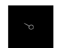
Figure 2: Samples of the academic dataset consisting of randomly affine-transformed synthetic template images.

class 1	class 5	class 7

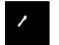
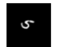
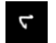
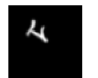
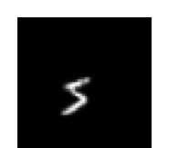
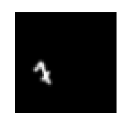
Figure 3: Samples of the LinMNIST dataset (random choices of ones, fifths and sevens) based on affine-transformed MNIST digits.

Table 2: Accuracy of nearest neighbor classification for the academic dataset with 10 images per class and the LinMNIST dataset with 50 images per class.

num.	academic		LinMNIST
angles	$\|\cdot\|_{\infty}$	$\|\cdot\|_{2}$	$\|\cdot\|_{\infty}$	$\|\cdot\|_{2}$
2	0.76	1.00	$0.540\pm 0.126$	$0.591\pm 0.130$
4	0.83	0.93	$0.565\pm 0.104$	$0.642\pm 0.105$
8	1.00	1.00	$0.644\pm 0.120$	$0.726\pm 0.119$
16	1.00	1.00	$0.654\pm 0.115$	$0.726\pm 0.120$
32	1.00	1.00	$0.655\pm 0.121$	$0.721\pm 0.120$
64	1.00	1.00	$0.656\pm 0.119$	$0.724\pm 0.119$
128	1.00	1.00	$0.656\pm 0.121$	$0.721\pm 0.116$

Figure 4: Visualization of _mNR-CDT for the academic dataset and 128 angles in $[0,\pi)$.

4.1 Nearest Neighbour Classification

In the first experiment, we aim to validate the theoretical result from Theorem 3.1. Looking at the proof, we recall that _mNR-CDT maps each entire affine class to a single point. The easiest way for classification is the nearest neighbor method, which can be immediately generalized to an arbitrary number of classes. For the first dataset, we use the template symbols as references and classify all class members based on the nearest neighbour rule with respect to the Chebychev and Euclidean norm, cf. Table 2 (columns 2 and 3) for qualitative results. For illustration, the _mNR-CDT of all considered classes are depicted in Figure 4. In theory, the classes should yield three curves. However, due to approximation errors, we observe slight perturbations. For the second dataset, since we have no templates, we iteratively select one instance per class as reference and classify the remaining class members again based on the nearest neighbour rule. Thereon, we compute the mean and standard deviation of the achieved accuracy, see Table 2 (columns 4 and 5). For the discretization of the _mNR-CDT, we use $2$ to $128$ angles in $[0,\pi)$, reported in column 1 of Table 2. As expected, due to Theorem 3.1, the classification of the first dataset is (nearly) perfect; remarkable, already for a very small number of chosen angles. For the LinMNIST dataset, the achieved accuracy ranges from $55\%$ to $73\%$, which is still significantly better than random guessing, achieving an accuracy of $33\%$ as we deal with a three class problem. Let us stress that perfect classification is not to be expected since LinMNIST does not satisfy our theoretical assumptions.

4.2 Support Vector Machine Classification

Table 3: Classification accuracy (mean$\pm$std based on $10$-fold cross validation) for the academic dataset. The first two classes in Fig. 2 are used with different class sizes and numbers of equispaced angles in $[0,\pi)$.

class	Euclidean	R-CDT				mNR-CDT
size		2	4	8	16	2	4	8	16
10	$0.489\pm 0.097$	$0.644\pm 0.112$	$0.572\pm 0.079$	$0.567\pm 0.086$	$0.561\pm 0.076$	$0.872\pm 0.114$	$0.806\pm 0.092$	$0.944\pm 0.082$	$\mathbf{0.989\pm 0.023}$
30	$0.520\pm 0.092$	$0.825\pm 0.128$	$0.728\pm 0.089$	$0.704\pm 0.065$	$0.704\pm 0.080$	$0.956\pm 0.094$	$0.979\pm 0.051$	$\mathbf{1.000\pm 0.000}$	$\mathbf{1.000\pm 0.000}$
90	$0.551\pm 0.028$	$0.962\pm 0.036$	$0.952\pm 0.056$	$0.974\pm 0.043$	$0.982\pm 0.041$	$0.996\pm 0.008$	$0.990\pm 0.009$	$\mathbf{1.000\pm 0.000}$	$\mathbf{1.000\pm 0.000}$
270	$0.610\pm 0.021$	$0.997\pm 0.006$	$0.999\pm 0.001$	$\mathbf{1.000\pm 0.000}$	$\mathbf{1.000\pm 0.000}$	$\mathbf{1.000\pm 0.000}$	$\mathbf{1.000\pm 0.000}$	$\mathbf{1.000\pm 0.000}$	$\mathbf{1.000\pm 0.000}$

Table 4: Classification accuracy (mean$\pm$std based on $10$-fold cross validation) for the LinMNIST dataset. The first and last class in Fig. 3 are used with different class sizes and numbers of equispaced angles in $[0,\pi)$.

class	Euclidean	R-CDT				mNR-CDT
size		4	8	16	32	4	8	16	32
10	$0.478\pm 0.070$	$0.611\pm 0.047$	$0.556\pm 0.027$	$0.556\pm 0.035$	$0.556\pm 0.027$	$0.794\pm 0.064$	$\mathbf{0.833\pm 0.091}$	$0.816\pm 0.059$	$0.822\pm 0.063$
20	$0.528\pm 0.057$	$0.583\pm 0.023$	$0.583\pm 0.037$	$0.583\pm 0.027$	$0.583\pm 0.026$	$0.842\pm 0.050$	$\mathbf{0.883\pm 0.039}$	$0.877\pm 0.035$	$0.881\pm 0.039$
50	$0.653\pm 0.044$	$0.756\pm 0.037$	$0.844\pm 0.060$	$0.878\pm 0.072$	$0.822\pm 0.047$	$0.890\pm 0.044$	$0.927\pm 0.024$	$0.932\pm 0.025$	$\mathbf{0.936\pm 0.022}$
250	$0.898\pm 0.024$	$0.945\pm 0.025$	$0.949\pm 0.016$	$0.953\pm 0.010$	$0.957\pm 0.012$	$0.955\pm 0.013$	$0.962\pm 0.008$	$0.964\pm 0.005$	$\mathbf{0.966\pm 0.005}$
500	$0.940\pm 0.010$	$0.948\pm 0.010$	$0.950\pm 0.006$	$0.949\pm 0.005$	$0.952\pm 0.007$	$0.950\pm 0.005$	$0.961\pm 0.009$	$0.963\pm 0.005$	$\mathbf{0.964\pm 0.005}$
1.000	$0.959\pm 0.005$	$0.939\pm 0.007$	$0.945\pm 0.008$	$0.948\pm 0.008$	$0.949\pm 0.009$	$0.949\pm 0.006$	$0.961\pm 0.007$	$0.965\pm 0.005$	$\mathbf{0.966\pm 0.006}$
5.000	$\mathbf{0.977\pm 0.003}$	$0.947\pm 0.003$	$0.956\pm 0.002$	$0.958\pm 0.002$	$0.962\pm 0.002$	$0.956\pm 0.002$	$0.969\pm 0.001$	$0.973\pm 0.001$	$0.974\pm 0.004$

In this second set of numerical experiments, we compare three different ansätze in combination with linear support vector machines (SVMs). The naïve approach uses the Euclidean representation of the images as basis for the SVM. Inspired by [7], the second approach makes use of the plain R-CDT projections using a fixed number of angles. Finally, the third approach utilizes our _mNR-CDT projections over the same set of angles. For all these methods, a $10$-fold cross validation is performed. This means that the dataset is partitioned into ten subsets, of which one is successively used for training, whereas the remaining nine are reserved for testing. The results for different class sizes and numbers of angels are summarized for the academic dataset in Table 3 and for the LinMNIST dataset in Table 4. We observe that our approach outperforms all others, especially in the small data regime and for few angles. For large data sizes, all methods perform at nearly the same accuracy.

5 Conclusion

In this work, we proposed the novel max-normalized R-CDT for feature representation and proved linear separability of classes generated by affine transforms of given templates. This was validated by numerical experiments showing a significant increase in classification accuracy over original R-CDT. Potential future directions include the control of perturbations either in the templates or in the transforms as well as a more in-depth numerical study in various applications.

References

• [1] Beckmann, M., Heilenkötter, N.: Equivariant neural networks for indirect measurements. SIAM Journal on Mathematics of Data Science 6(3), 579–601 (2024). https://doi.org/10.1137/23M1582862
• [2] Beier, F., Beinert, R., Steidl, G.: On a linear Gromov–Wasserstein distance. IEEE Transactions on Image Processing 31, 7292–7305 (2022). https://doi.org/10.1109/TIP.2022.3221286
• [3] Bonneel, N., Rabin, J., Peyré, Pfister, H.: Sliced and Radon Wasserstein barycenters of measures. Journal of Mathematical Imaging and Vision 51(1), 22–45 (2015). https://doi.org/10.1007/s10851-014-0506-3
• [4] Deng, L.: The MNIST database of handwritten digit images for machine learning research. IEEE Signal Processing Magazine 29(6), 141–142 (2012). https://doi.org/10.1109/MSP.2012.2211477
• [5] Diaz Martin, R., Medri, I.V., Rohde, G.K.: Data representation with optimal transport (2024). https://doi.org/10.48550/arXiv.2406.15503, arXiv:2406.15503
• [6] Hauser, D., Beckmann, M., Koliander, G., Stiehl, H.S.: On image processing and pattern recognition for thermograms of watermarks in manuscripts – a first proof-of-concept. In: International Conference on Document Analysis and Recognition (ICDAR). pp. 91–107 (2024). https://doi.org/10.1007/978-3-031-70543-4_6
• [7] Kolouri, S., Park, S.R., Rohde, G.K.: The Radon cumulative distribution transform and its application to image classification. IEEE Transactions on Image Processing 25(2), 920–934 (2016). https://doi.org/10.1109/TIP.2015.2509419
• [8] Kolouri, S., Park, S.R., Thorpe, M., Slepcev, D., Rohde, G.K.: Optimal mass transport. IEEE Signal Processing Magazine 34(4), 43–59 (2017). https://doi.org/10.1109/MSP.2017.2695801
• [9] Moosmüller, C., Cloninger, A.: Linear optimal transport embedding: provable Wasserstein classification for certain rigid transformations and perturbations. Information and Inference: A Journal of the IMA 12(1), 363–389 (2023). https://doi.org/10.1093/imaiai/iaac023
• [10] Natterer, F.: The Mathematics of Computerized Tomography. SIAM, Philadelphia (2001). https://doi.org/10.1137/1.9780898719284
• [11] Quellmalz, M., Beinert, R., Steidl, G.: Sliced optimal transport on the sphere. Inverse Problems 39(10), 105005 (2023). https://doi.org/10.1088/1361-6420/acf156
• [12] Quellmalz, M., Buecher, L., Steidl, G.: Parallelly sliced optimal transport on spheres and on the rotation group. Journal of Mathematical Imaging and Vision 66(6), 951–976 (2024). https://doi.org/10.1007/s10851-024-01206-w
• [13] Ramm, A.G., Katsevich, A.I.: The Radon Transform and Local Tomography. CRC Press (1996). https://doi.org/10.1201/9781003069331
• [14] Shifat-E-Rabbi, M., Yin, X., Rubaiyat, A.H.M., Li, S., Kolouri, S., Aldroubi, A., Nichols, J.M., Rohde, G.K.: Radon cumulative distribution transform subspace modeling for image classification. Journal of Mathematical Imaging and Vision 63, 1185–1203 (2021). https://doi.org/10.1007/s10851-021-01052-0
• [15] Shifat-E-Rabbi, M., Zhuang, Y., Li, S., Rubaiyat, A.H.M., Yin, X., Rohde, G.K.: Invariance encoding in sliced-Wasserstein space for image classification with limited training data. Pattern Recognition 137, 109268 (2023). https://doi.org/10.1016/j.patcog.2022.109268
• [16] Villani, C.: Topics in Optimal Transportation. American Mathematical Society (2003). https://doi.org/10.1090/gsm/058