Quantum Relay Channels

Abstract

Communication over a fully quantum relay channel is considered. We establish three bounds based on different coding strategies, i.e., partial decode-forward, measure-forward, and assist-forward. Using the partial-decode forward strategy, the relay decodes part of the information, while the other part is decoded without the relay’s help. The result by Savov et al. (2012) for a classical-quantum relay channel is obtained as a special case. Based on our partial-decode forward bound, the capacity is determined for Hadamard relay channels. In the measure-forward coding scheme, the relay performs a sequence of measurements and then sends a compressed representation of the measurement outcome to the destination receiver. The measure-forward strategy can be viewed as a generalization of the classical compress-forward bound. At last, we consider quantum relay channels with orthogonal receiver components. The assist-forward bound is based on a new approach, whereby the transmitter sends the message to the relay and simultaneously generates entanglement assistance between the relay and the destination receiver. Subsequently, the relay can transmit the message to the destination receiver with rate-limited entanglement assistance.

Figure 1: A three-terminal relay network.

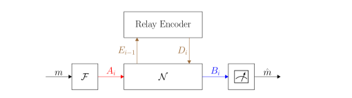
Figure 2: Coding for a fully quantum relay channel $\mathcal{N}_{AD\rightarrow BE}$. The quantum systems of Alice, Bob, and the relay are marked in red, blue, and brown, respectively.

I Introduction

Relaying plays a crucial role in enabling long-range communication. For example, in free-space optics systems, the transmission distance is limited by atmospheric conditions, including absorption, scattering, and turbulence [1]. Attenuation in optical fibers poses a significant challenge as well. By dividing a communication link into two segments and placing a relay terminal between them, one can rectify problems such as photon loss and operation defects [2]. Relaying is thus considered a promising and effective solution [3]. Optimists view this solution as a key step toward quantum-enabled 6G communication [4]. Furthermore, in the long-term vision of an ad-hoc network of the quantum Internet [5], any node could act both as a transceiver of data and as a relay for other transmissions [6].

Cooperation in quantum communication networks has become a major focus of study in recent years, driven by advances in experimental techniques and theoretical insights [7, 8, 9, 10, 11]. Entanglement is a valuable resource in network communication [12]. In the point-to-point setting, entanglement assistance between the transmitter and the receiver can significantly increase throughput [13], even if the resource is noisy [14] or unreliable [15]. Entanglement assistance has recently been considered under the security requirements of secrecy [16, 17, 18] and covertness [19, 20, 21] as well. In multi-user networks, entanglement between transmitters can also increase achievable rates for classical multiple-access channels [22, 23, 24], and yet entanglement between receivers improves neither achievable rates [25], nor error probabilities [26], for broadcast channels. The three-terminal relay channel in Figure 1 is a fundamental unit in user cooperation as well [27], and can also be used to generate entanglement between network nodes [28].

In a multihop network, there are multiple rounds of communication, thus, synchronization is important [29, 30]. Suppose that the operation is governed by a central clock that ticks $n$ times. Between the clock ticks $i-1$ and $i$, the sender and the relay transmit the channel inputs $A_{i}$ and $D_{i}$, respectively. See Figure 2. Then, at the clock tick $i$, the relay and destination receivers receive the channel outputs $E_{i}$ and $B_{i}$. This requires a small delay before reception to ensure causality. The classical channel model was originally introduced by van der Meulen [31] as a building block for multihop networks [32].

Savov et al. [33, 34] considered classical-quantum (c-q) relay channels and derived a partial decode-forward achievable rate for sending classical information. In the c-q case, both $A_{i}$ and $D_{i}$ are classical. Boche et al. [35] considered a c-q model of two-phase bidirectional relaying. Communication with the help of environment measurement can be viewed as a quantum channel with a classical relay in the environment [36]. Considering this setting, Smolin et al. [37] and Winter [38] determined the environment-assisted quantum capacity and classical capacity, respectively. Furthermore, Ding et al. [39] established the cutset, multihop, and coherent multihop bounds on the capacity of the c-q relay channel. To the best of our knowledge, a fully quantum channel was not considered.

Network settings with causality aspects often require block Markov coding [40], where the transmitter sends a sequence of blocks, and each block transmission encodes descriptions that are associated with the current and previous blocks. Quantum versions of block Markov coding were previously used for c-q relay channels [33, 34], communication with parameter estimation at the receiver [41], and quantum cribbing between transmitters [42].

Sending quantum information is outside the scope of the present work, as we focus here on the classical task of sending a classical message. Nonetheless, we note that in order to distribute entanglement and send quantum information, the quantum relay would need to operate as a quantum repeater [43]. Pereg et al. [25] addressed transmission of quantum information via a primitive relay channel, with a noiseless qubit pipe from the relay to the destination receiver, and provided an information-theoretic perspective on quantum repeaters. Other relay channel models for quantum repeaters can also be found in [44, 45, 46, 47, 48].

We consider the transmission of messages via a fully quantum relay channel. As opposed to previous work [33, 34, 35, 39], the channel is fully quantum. We establish three bounds based on different coding strategies, i.e., partial decode-forward, measure-forward, and assist-forward. Using the partial-decode forward strategy, the relay decodes part of the information, while the other part is decoded without the relay’s help. Based on our partial-decode forward bound, we determine the capacity for the special class of Hadamard relay channels. We also recover the result by Savov et al. [33] for the special case of a c-q relay channel. In the measure-forward coding scheme, the relay performs a sequence of measurements and then sends a compressed representation of the measurement outcome to the destination receiver. The measure-forward strategy can be viewed as a generalization of the classical compress-forward bound due to Cover and El Gamal [49]. At last, we consider quantum relay channels with orthogonal receiver components. The assist-forward bound is based on a new approach, whereby the transmitter sends the message to the relay and simultaneously generates entanglement assistance between the relay and the destination receiver. Subsequently, the relay can transmit the message to the destination receiver with rate-limited entanglement assistance. We demonstrate our results by computing a closed-form lower bound for a depolarizing relay channel.

The paper is organized as follows. In Section II, we give preliminary definitions and present the channel model. Section III provides the coding definitions for communication with strictly causal quantum relaying. Section IV presents our main results, including the partial decode-forward, measure-forward, and assist-forward bounds. In Section V, we give examples. Section VI concludes with a summary and discussion. The analysis is given in the appendix. Appendix A provides information-theoretic tools. In Appendices B through E, we derive the partial decode-forward, measure-forward, and assist-forward bounds, with Appendix C addressing Hadamard relay channels.

II Definitions and Channel Model

II-A Notation, States, and Information Measures

We use the following notation conventions. Script letters $\mathcal{X},\mathcal{Y},\mathcal{Z},...$ are used for finite sets. Lowercase letters $x,y,z,\ldots$ represent constants and values of classical random variables, and uppercase letters $X,Y,Z,\ldots$ represent classical random variables. The distribution of a random variable $X$ is specified by a probability mass function (pmf) $p_{X}(x)$ over a finite set $\mathcal{X}$. We use $x^{j}=(x_{1},x_{2},\ldots,x_{j})$ to denote a sequence of letters from $\mathcal{X}$. A random sequence $X^{n}$ and its distribution $p_{X^{n}}(x^{n})$ are defined accordingly.

A quantum state is described by a density operator $\rho$ on the Hilbert space $\mathcal{H}$. The dimensions are assumed to be finite. We denote the set of all such density operators by $\mathfrak{D}(\mathcal{H})$. The probability distribution of a measurement outcome can be described in terms of a positive operator-valued measure (POVM), i.e. a set of positive semidefinite operators $\{\Delta_{j}\}$, such that $\sum_{j}\Delta_{j}=\mathbbm{1}$, where $\mathbbm{1}$ is the identity operator. According to the Born rule, if the system is in state $\rho$, then the probability of the measurement outcome $j$ is given by $\Pr(j)=\mathrm{Tr}(\Delta_{j}\rho)$.

Define the quantum entropy of the density operator $\rho$ as $H(\rho)\equiv-\mathrm{Tr}[\rho\log(\rho)]$, which is the same as the Shannon entropy associated with the eigenvalues of $\rho$. Consider the state of a pair of systems $A$ and $B$ on the tensor product $\mathcal{H}_{A}\otimes\mathcal{H}_{B}$ of the corresponding Hilbert spaces. Given a bipartite state $\rho_{AB}$, define the quantum mutual information as

$$I(A;B)_{\rho}=H(\rho_{A})+H(\rho_{B})-H(\rho_{AB})\,.$$ (1)

Furthermore, conditional quantum entropy and mutual information are defined by $H(A|B)_{\rho}=H(\rho_{AB})-H(\rho_{B})$ and $I(A;B|C)_{\rho}=H(A|C)_{\rho}+H(B|C)_{\rho}-H(AB|C)_{\rho}$, respectively. The coherent information is then defined as

$$I(A\rangle B)_{\rho}=-H(A|B)_{\rho}\,.$$ (2)

Figure 3: A diagram of the quantum relay channel: The transmitters at the sender and the relay are labeled as $A$ and $D$, and the receivers at the destination and the relay as $B$ and $E$, respectively.

II-B Channel Model

We consider a fully quantum relay channel as a model for the three-terminal network in Figure 1. A quantum relay channel is a completely-positive trace-preserving (CPTP) map, $\mathcal{N}_{AD\rightarrow BE}$, where $A$, $D$, $B$, and $E$ are associated with the sender transmitter, the relay transmitter, the destination receiver, and the relay receiver, respectively. See Figure 3. We assume that the channel is memoryless. That is, if the systems $A^{n}=(A_{1},\ldots,A_{n})$ and $D^{n}=(D_{1},\ldots,D_{n})$ are sent through $n$ channel uses, then the input state $\rho_{A^{n}D^{n}}$ undergoes the tensor product mapping

$$\mathcal{N}_{A^{n}D^{n}\rightarrow B^{n}E^{n}}\equiv(\mathcal{N}_{AD\rightarrow BE})^{\otimes n}\,.$$ (3)

The communication setting will be defined in Section III such that the relay encodes in a strictly causal manner. That is, the relay transmits $D_{i}$ at time $i$, and only then receives $E_{i}$.

II-C Special Cases

We will also discuss the special class of degraded relay channels. Intuitively, if a relay channel is degraded, then the output of the destination receiver is a noisy version of that of the relay. In practice, this is typically the case, since the relay is an intermediate station between the transmitter and the destination receiver.

Let $\mathcal{M}_{AD\to E}$ denote the marginal channel to the relay, and $\mathcal{L}_{AD\to B}$ to the destination receiver:

$$\mathcal{M}_{AD\to E} =\mathrm{Tr}_{B}\circ\mathcal{N}_{AD\to BE}\,,$$ (4)

$$\mathcal{L}_{AD\to B} =\mathrm{Tr}_{E}\circ\mathcal{N}_{AD\to BE}\,.$$ (5)

Definition 1 (Degraded relay channel).

A quantum relay channel $\mathcal{N}_{AD\rightarrow BE}$ is called degraded if there exists a degrading channel $\mathcal{P}_{E\rightarrow B}$ such that the marginals satisfy the following relation,

$$\mathcal{L}_{AD\to B}=\mathcal{P}_{E\to B}\circ\mathcal{M}_{AD\to E}\,.$$ (6)

In this case, we say that Bob’s channel $\mathcal{L}_{AD\to B}$ is degraded with respect to the relay’s channel, $\mathcal{M}_{AD\to E}$.

We also introduce the definition of a Hadamard relay channel. In this case, the relay receives a classical observation $Y_{1}$, which can be interpreted as a measurement outcome.

Definition 2.

A Hadamard relay channel $\mathcal{N}^{\,\text{H}}_{AD\rightarrow BY_{1}}$ is a quantum-quantum-quantum-classical relay channel that is also degraded, i.e.,

$$\mathcal{L}_{AD\to B}=\mathcal{P}_{Y_{1}\to B}\circ\mathcal{M}_{AD\to Y_{1}}$$ (7)

where $Y_{1}$ is classical.

Intuitively, if a relay channel is degraded, then the output state of the destination receiver is a noisy version of that of the relay. For a Hadamard relay channel $\mathcal{N}^{\,\text{H}}_{AD\to BY_{1}}$, the relay can be viewed as a measure-and-prepare device. The marginal channel $\mathcal{M}_{AD\rightarrow Y_{1}}$ acts as a measurement device, while the degrading channel $\mathcal{P}_{Y_{1}\rightarrow B}$ corresponds to state preparation.

In this case, Bob’s channel $\mathcal{L}_{AD\rightarrow B}$ is said to be entanglement-breaking [50]. The map $\mathcal{N}^{\,\text{H}}_{AD\rightarrow BY_{1}}$ can also be viewed as a Hadamard broadcast channel [51, 25], where Bob and the relay are interpreted as two receivers.

III Coding

We consider a fully quantum relay channel $\mathcal{N}_{AD\to BE}$. Below, we define a code for the transmission of classical information via the quantum relay channel. The relay serves the purpose of assisting the transmission of information from Alice to Bob.

Definition 3.

A $(2^{nR},n)$ classical code for the quantum relay channel $\mathcal{N}_{AD\to BE}$ consists of the following:

• A message set $[1:2^{nR}]$, where $2^{nR}$ is assumed to be an integer,

• an encoding map $\mathcal{F}_{M\rightarrow A^{n}}:[1:2^{nR}]\to\mathfrak{D}(\mathcal{H}_{A}^{\otimes n})$,

• a sequence of strictly-causal relay encoding maps $\Gamma^{(i)}_{E_{i-1}\bar{E}^{i-2}\rightarrow\bar{E}^{i-1}D_{i}}:\mathfrak{D}(\mathcal{H}_{E}^{\otimes(i-1)})\to\mathfrak{D}(\mathcal{H}_{E}^{\otimes(i-1)}\otimes\mathcal{H}_{D})$, for $i\in[1:n]$,

• a decoding POVM $\{\Delta_{m}\}$ on $\mathcal{H}_{B}^{\otimes n}$, where the measurement outcome $m$ is an index in $[1:2^{nR}]$.

We denote the code by $(\mathcal{F},\Gamma,\Delta)$.

The communication scheme is depicted in Figure 2. The systems $A^{n}$ and $D^{n}$ represent the transmissions by the sender and the relay, respectively. Whereas, $E^{n}$ and $B^{n}$ are the received outputs at the relay and the destination receiver, respectively. Alice selects a uniform message $m\in[1:2^{nR}]$ that is intended for the destination receiver, Bob. She encodes the message by applying the encoding map $\mathcal{F}_{M\to A^{n}}$, and transmits the systems $A^{n}$ over $n$ channel uses.

At time $i$, the relay applies the encoding map $\Gamma^{(i)}_{E_{i-1}\bar{E}^{i-2}\rightarrow\bar{E}^{i-1}D_{i}}$ to $E_{i-1},\bar{E}^{i-2}$, and then receives $E_{i}$, for $i\in[1:n]$. The system $\bar{E}^{i-1}$ can be viewed as a “leftover" of the encoding operation at time $i$. Specifically, at time $i=1$, we have

$$\rho_{A^{n}D_{1}}^{(m)} =\mathcal{F}_{M\to A^{n}}(m)\otimes\Gamma^{(1)}_{E_{0}\to D_{1}}(1)\,,$$ (8)

where $$E_{0} 1 A^{n} A_{1} A_{2}^{n}\equiv(A_{i})_{i\geq 2} E_{1}$$ is a degenerate system of dimension . We now split into and . Then, the relay receives in the state

$$\rho_{B_{1}E_{1}A_{2}^{n}}^{(m)} =\left(\mathcal{N}_{AD\to BE}\otimes\mathrm{id}_{A_{2}^{n}}\right)(\rho_{A_{1}D_{1}A_{2}^{n}}^{(m)})\,.$$ (9)

At time $i=2$, the relay encodes $D_{2}$ by

$$\rho_{\bar{E}_{1}D_{2}A_{2}^{n}B_{1}}^{(m)} =\left(\Gamma^{(2)}_{E_{1}\rightarrow\bar{E}_{1}D_{2}}\otimes\mathrm{id}_{A_{2}^{n}B_{1}}\right)(\rho_{E_{1}A_{2}^{n}B_{1}}^{(m)})\,,$$ (10)

where $$\bar{E}_{1} E_{2}$$ is a leftover that can be used in subsequent steps. The relay receives in the state

$$\rho_{B_{2}E_{2}A_{3}^{n}B_{1}\bar{E}_{1}}^{(m)} =(\mathcal{N}_{AD\to BE}\otimes\mathrm{id}_{A_{3}^{n}B_{1}\bar{E}_{1}})(\rho_{A_{2}D_{2}A_{3}^{n}B_{1}\bar{E}_{1}}^{(m)})\,.$$ (11)

This continues in the same manner. At time $i=n$, the relay encodes by

$$\rho_{\bar{E}^{n-1}D_{n}A_{n}B^{n-1}}^{(m)} =\left(\Gamma^{(n)}_{E_{n-1}\bar{E}^{n-2}\to\bar{E}^{n-1}D_{n}}\otimes\mathrm{id}_{A_{n}B^{n-1}}\right)(\rho_{E_{n-1}\bar{E}^{n-2}A_{n}B^{n-1}}^{(m)})\,,$$ (12)

and then,

$$\rho_{B^{n}E_{n}\bar{E}^{n-1}}^{(m)} =(\mathcal{N}_{AD\to BE}\otimes\mathrm{id}_{B^{n-1}\bar{E}^{n-1}})(\rho_{A_{n}D_{n}B^{n-1}\bar{E}^{n-1}}^{(m,s)})\,.$$ (13)

Thus, the output state at the destination receiver is the reduced state, $\rho_{B^{n}}^{(m)}=\mathrm{Tr}_{E_{n}\bar{E}^{n-1}}\left(\rho_{B^{n}E_{n}\bar{E}^{n-1}}^{(m)}\right)$.

Bob receives the channel output system $B^{n}$, performs the measurement $\{\Delta_{m}\}$, and obtains an estimate $\hat{m}\in[1:2^{nR}]$ of Alice’s message, as the measurement outcome. The average probability of error of the code $(\mathcal{F},\Gamma,\Delta)$ is given by

$$P_{e}^{(n)}(\mathcal{F},\Gamma,\Delta) =1-\frac{1}{2^{nR}}\sum_{m=1}^{2^{nR}}\mathrm{Tr}(\Delta_{m}\rho^{(m)}_{B^{n}})\,.$$ (14)

A $(2^{nR},n,\varepsilon)$ code for the quantum relay channel satisfies $P_{e}^{(n)}(\mathcal{F},\Gamma,\Delta)\leq\varepsilon$. A rate $R\geq 0$ is called achievable if for every $\varepsilon,\delta>0$ and sufficiently large $n$, there exists a $(2^{n(R-\delta)},n,\varepsilon)$ code. Equivalently, $R$ is achievable if there exists a sequence of codes at rate $R-\delta$ such that the average probability of error tends to zero as $n\to\infty$, where $\delta>0$ is arbitrarily small.

The capacity of the quantum relay channel $C(\mathcal{N})$ is defined as the supremum of achievable rates.

Remark 1.

The relay is only required to assist the transmission of information to Bob, and does not necessarily decode any information. In particular, we will later introduce a measure-forward strategy where the relay does not decode information at all. See Section IV-B below.

Remark 2.

The code definition above for the quantum setting is somewhat more involved than in previous work [33, 34, 35, 39], since we need to account for the post-operation state at the relay in each time instance. That is, the relay encoding at time $i$ affects the state of $E_{i-1}$, as well as the previous outputs. As mentioned above, the system $\bar{E}^{i-1}$ can be viewed as a “leftover" of the relay encoding at time $i$. This leftover can be used in subsequent steps, at time $j>i$. For example, if the relay performs a sequence of measurements, then $\Gamma^{(i)}$ are quantum instruments such that $\bar{E}^{i-1}$ is the post-measurement system, while $D_{i}$ stores the measurement outcome. In the classical setting, $\bar{E}^{i-1}$ is simply a copy of the previously received observations at the relay.

IV Main Results

Now, we give our results on the quantum relay channel $\mathcal{N}_{AD\to BE}$. We will establish achievable rates that are based on different coding strategies. We will also discuss special cases in which those strategies achieve the capacity of the quantum relay channel.

IV-A Partial Decode-Forward Strategy

In the partial decode-forward strategy, the relay decodes part of the information, while the other part is decoded without the relay’s help. Our derivation can be viewed as a quantum version of the classical coding strategy, under the same name [49]. Let

$$\mathsf{R}_{\text{PD-F}}(\mathcal{N})\equiv\max_{p_{UX_{0}X_{1}}\,,\;\theta^{x_{0}}_{A}\otimes\zeta^{x_{1}}_{D}}\min\bigg{\{} I(X_{0}X_{1};B)_{\omega}\,,\;I(U;E|X_{1})_{\omega}+I(X_{0};B|X_{1}U)_{\omega}\bigg{\}}$$ (15)

where the maximum is over the set of all probability distributions $p_{UX_{0}X_{1}}(u,x_{0},x_{1})$ and product state collections $\{\theta^{x_{0}}_{A}\otimes\zeta^{x_{1}}_{D}\}$, with

$$\omega_{UX_{0}X_{1}BE}=\sum_{(u,x_{0},x_{1})\in\mathcal{U}\times\mathcal{X}_{0}\times\mathcal{X}_{1}}p_{UX_{0}X_{1}}(u,x_{0},x_{1})\outerproduct{u}{u}\otimes\outerproduct{x_{0}}{x_{0}}\otimes\outerproduct{x_{1}}{x_{1}}\otimes\mathcal{N}_{AD\rightarrow BE}(\theta^{x_{0}}_{A}\otimes\zeta^{x_{1}}_{D})\,.$$ (16)

Remark 3.

The random variable $U$ represents the information that is decoded by the relay, which gives rise to the mutual information term $I(U;E|X_{1})$. The other terms are associated with the decoding at the destination receiver.

Remark 4.

Taking $U$ to be null, we obtain the direct-transmission lower bound:

$$\mathsf{R}_{\text{PD-F}}(\mathcal{N})\geq\max_{p_{X_{0}}\,,\;\theta^{x_{0}}_{A}\otimes\outerproduct{\zeta_{D}}{\zeta_{D}}}I(X_{0};B)_{\omega}\,.$$ (17)

As expected, the direct-transmission lower bound is the Holevo information [52]. To achieve this bound, the relay does not need to decode anything. On the other hand, by taking $U=X_{0}$, we obtain

$$\mathsf{R}_{\text{PD-F}}(\mathcal{N})\geq\max_{p_{X_{0}X_{1}}\,,\;\theta^{x_{0}}_{A}\otimes\zeta^{x_{1}}_{D}}\min\bigg{\{} I(X_{0}X_{1};B)_{\omega}\,,\;I(X_{0};E|X_{1})_{\omega}\bigg{\}}\,.$$ (18)

This bound is achieved through a full decode-forward coding strategy, where the relay decodes the entire information. As can be seen in the formula, this induces a bottleneck behavior.

Our first capacity result is given in the theorem below.

Theorem 1.

The capacity of the quantum relay channel $\mathcal{N}_{AD\to BE}$ satisfies

$$C(\mathcal{N})\geq\mathsf{R}_{\text{PD-F}}(\mathcal{N})\,.$$ (19)

The proof of Theorem 1 is given in Appendix B. Next, we consider three special classes.

IV-A1 Classical-quantum channel

As a special case, we recover the result by Savov et al. [33], for a classical-quantum channel. Here, the transmissions $A$ and $D$ are replaced by classical transmissions, $X$ and $X_{1}$, respectively.

Corollary 2 (see [33, Th. 1]).

For a classical-quantum relay channel $\mathcal{N}_{XX_{1}\to BE}$,

$$C(\mathcal{N})\geq\max_{p_{UXX_{1}}}\min\bigg{\{} I(XX_{1};B)_{\omega}\,,\;I(U;E|X_{1})_{\omega}+I(X;B|X_{1}U)_{\omega}\bigg{\}}\,.$$ (20)

where the maximum is over the set of all probability distributions $p_{UXX_{1}}(u,x,x_{1})$, with

$$\omega_{UXX_{1}BE}=\sum_{(u,x,x_{1})\in\mathcal{U}\times\mathcal{X}\times\mathcal{X}_{1}}p_{UXX_{1}}(u,x,x_{1})\outerproduct{u}{u}\otimes\outerproduct{x}{x}\otimes\outerproduct{x_{1}}{x_{1}}\otimes\mathcal{N}_{XX_{1}\rightarrow BE}(x,x_{1})\,.$$ (21)

Remark 5.

In particular, one may consider the trivial case of an anti-degradable channel. Suppose that there exist reversely-degrading channels $\{\bar{\mathcal{P}}^{(x_{1})}_{B\to E}\}$ such that

$$\mathcal{M}_{XX_{1}\to E}(x,x_{1})=\left(\bar{\mathcal{P}}^{(x_{1})}_{B\to E}\circ\mathcal{L}_{XX_{1}\to B}\right)(x,x_{1})$$ (22)

for all input pairs $(x,x_{1})$. Intuitively, the direct channel to the destination receiver is better than the channel to the relay, and thus, the relay is useless. As expected, the capacity is

$$C(\mathcal{N})=\max_{x_{1}\in\mathcal{X}_{1}}\max_{p_{X}}I(X;B|X_{1}=x_{1})_{\omega}\,.$$ (23)

Achievability follows by taking $U$ to be null in (20) (see Remark 4). The converse proof is straightforward as well, based on standard arguments.

IV-A2 Hadamard relay channel

Now, suppose the encoder and the relay both have quantum transmissions, $A$ and $D$, respectively, and the decoder receives a quantum system $B$. However, the relay receives a classical observation $Y_{1}$, which can be interpreted as a measurement outcome. Recall from Subsection II-C, that a Hadamard relay channel is also degraded. In this case, the relay can be interpreted as a measure-and-prepare device.

Theorem 3.

The capacity of a Hadamard relay channel $\mathcal{N}_{AD\to BY_{1}}$, as in Definition 2, is given by

$$C(\mathcal{N})=\max_{p_{X_{0}X_{1}}\,,\;\theta^{x_{0}}_{A}\otimes\zeta^{x_{1}}_{D}}\min\bigg{\{} I(X_{0}X_{1};B)_{\omega}\,,\;I(X_{0};Y_{1}|X_{1})_{\omega}\bigg{\}}$$ (24)

where the maximum is as in (15).

The proof for Theorem 3 is given in Appendix C. Essentially, Theorem 3 says that the full decode-forward strategy is optimal (see Remark 4). That is, the capacity is achieved when the relay decodes the entire information. This is intuitive since for a Hadamard relay channel, the relay’s channel is better than Bob’s channel.

IV-A3 Stinespring Dilation

Suppose that the quantum relay channel $\mathcal{N}_{AD\to BE}$ is a Stinespring dilation of the channel $\mathcal{L}_{AD\to B}$ to Bob, and thus the channel $\mathcal{M}_{AD\to E}$ to the relay is a complementary channel to $\mathcal{L}_{AD\to B}$. This means that the quantum relay channel can be represented by an isometry $V:\mathcal{H}_{A}\to\mathcal{H}_{B}\otimes\mathcal{H}_{E}$. The relay’s system $E$ can then be viewed as Bob’s environment. Furthermore, the full decode-forward bound yields the bound

$$C(\mathcal{N}) \geq\max_{p_{X_{0}}\,,\;\ket{\theta^{x_{0}}_{A}}\otimes\ket{\zeta_{D}}}\min\bigg{\{}H(B)_{\omega}\,,\;H(E)_{\omega}\bigg{\}}$$ (25)

which resembles the environment-assisted distillation rate in [37, Th. 1] (see [38] as well).

IV-B Measure-Forward Strategy

We introduce a new coding scheme, where the relay performs a sequence of measurements, and then sends a compressed representation of the measurement outcome. The relay does not decode any information in this coding scheme. This can be viewed as a quantum variation of the classical “compress-forward coding" approach [49]. Let

$$\mathsf{R}_{\text{M-F}}(\mathcal{N})\equiv\max I(X_{0};Z_{1}B|X_{1})_{\omega}$$ (26)

where the maximum is over the set of all product ensembles $\{p_{X_{0}},\theta^{x_{0}}_{A}\}$ $\otimes$ $\{p_{X_{1}},\zeta^{x_{1}}_{D}\}$, POVM collections $\mathcal{G}_{E\to Y_{1}}=\{\Gamma_{y_{1}}\}$, and classical channels $p_{Z_{1}|X_{1}Y_{1}}$ that satisfy

$$I(Z_{1};Y_{1}|X_{1}B)_{\omega}\leq I(X_{1};B)_{\omega}$$ (27)

for

$$\omega^{(x_{0},x_{1})}_{BE} =\mathcal{N}_{AD\rightarrow BE}(\theta^{x_{0}}_{A}\otimes\zeta^{x_{1}}_{D})\,,$$ (28)

$$\omega^{(x_{0},x_{1})}_{BY_{1}Z_{1}} =\sum_{y_{1}\in\mathcal{Y}_{1}}\bigg{[}\mathrm{Tr}_{E}\left\{\left(\mathbbm{1}\otimes\Gamma_{y_{1}}\right)\omega^{(x_{0},x_{1})}_{BE}\right\}\otimes\outerproduct{y_{1}}{y_{1}}\otimes$$

$$\sum_{z_{1}\in\mathcal{Z}_{1}}p_{Z_{1}|X_{1}Y_{1}}(z_{1}|x_{1},y_{1})\outerproduct{z_{1}}{z_{1}}\bigg{]}\,,$$ (29)

$$\omega_{X_{0}X_{1}BY_{1}Z_{1}} =\sum_{(x_{0},x_{1})\in\mathcal{X}_{0}\times\mathcal{X}_{1}}p_{X_{0}}(x_{0})p_{X_{1}}(x_{1})\outerproduct{x_{0}}{x_{0}}\otimes\outerproduct{x_{1}}{x_{1}}\otimes\omega^{(x_{0},x_{1})}_{BY_{1}Z_{1}}\,.$$ (30)

Remark 6.

Intuitively, the formula for $\mathsf{R}_{\text{M-F}}(\mathcal{N})$ above can be interpreted as follows. Given $x_{0}$ and $x_{1}$, the encoder and the relay prepare $\theta^{x_{0}}_{A}$ and $\zeta^{x_{1}}_{D}$, respectively. This results in the output state $\omega_{BE}^{(x_{0},x_{1})}$ in (28). The relay receives $E$ and performs a measurement, which yields $Y_{1}$ as an outcome. See (IV-B). The measurement outcome is then compressed and encoded by $Z_{1}$.

Roughly speaking, we interpret $nI(Z_{1};Y_{1}|X_{1}B)_{\omega}$ as the number of information bits that are obtained from the measurement compression operation, while the number of information bits that the relay can send through the channel to Bob is below $nI(X_{1};B)_{\rho}$. This limitation is reflected through the maximization constraint in (27).

Our measure-forward result is given below.

Theorem 4.

The capacity of the quantum relay channel $\mathcal{N}_{AD\to BE}$ satisfies

$$C(\mathcal{N})\geq\mathsf{R}_{\text{M-F}}(\mathcal{N})\,.$$ (31)

The proof of Theorem 4 is given in Appendix D.

IV-C Assist-Forward Strategy

We introduce a new approach, whereby Alice simultaneously sends the message to the relay and generates entanglement assistance between the relay and Bob. Subsequently, the relay communicates the message to Bob using rate-limited entanglement assistance. We consider a quantum relay channel with orthogonal receiver components (ORC), where Bob’s output has two components, i.e., $B=(B_{1},B_{2})$, and the quantum relay channel $\mathcal{N}_{AD\to B_{1}B_{2}E}$ has the following form:

$$\mathcal{N}_{AD\to B_{1}B_{2}E}=\mathcal{M}_{A\to B_{1}E}\otimes\mathcal{P}_{D\to B_{2}}\,.$$ (32)

Remark 7.

In words, the quantum relay channel $\mathcal{N}_{AD\to B_{1}B_{2}E}$ above is a product of two channels, a broadcast channel $\mathcal{M}_{A\to B_{1}E}$ from the sender to the relay and the receiver, and a direct channel $\mathcal{P}_{D\to B_{2}}$ from the relay to the receiver. The relay channel is referred to as having ORC due to this decoupling.

Consider the broadcast channel $\mathcal{M}_{A\to B_{1}E}$ from the sender to the relay and the receiver. Given an ensemble $\{p_{X_{1}},\theta^{x_{1}}_{G_{0}G_{1}A}\}$, let

$$Q(\mathcal{M},\theta) \equiv\min\left\{I(G_{0}\rangle B_{1}X_{1})_{\theta}\,,\;I(G_{1}\rangle EX_{1})_{\theta}\right\}\,.$$ (33)

Moving to the quantum relay channel $\mathcal{N}_{AD\to B_{1}B_{2}E}$ with ORC, define

$$\mathsf{R}_{\text{A-F}}(\mathcal{N}) \equiv\max_{\theta\otimes\zeta}\min\left\{I(X_{1};E)_{\theta}\,,\;I(X_{2}G_{2};B_{2})_{\zeta}\,,\;I(X_{2};B_{2})_{\zeta}+I(G_{2}\rangle B_{2}X_{2})_{\zeta}+Q(\mathcal{M},\theta)\right\}\,.$$ (34)

The maximum is over the set of all product ensembles $\{p_{X_{1}},\theta^{x_{1}}_{G_{0}G_{1}A}\}$ $\otimes$ $\{p_{X_{2}},\zeta^{x_{2}}_{G_{2}D}\}$, with

$$\theta_{X_{1}G_{0}G_{1}B_{1}E} =\sum_{x_{1}\in\mathcal{X}_{1}}p_{X_{1}}(x_{1})\outerproduct{x_{1}}{x_{1}}\otimes(\mathrm{id}_{G_{0}G_{1}}\otimes\mathcal{M}_{A\rightarrow B_{1}E})(\theta^{x_{1}}_{G_{0}G_{1}A})\,,$$ (35)

and

$$\zeta_{X_{2}G_{3}B_{2}} =\sum_{x_{2}\in\mathcal{X}_{2}}p_{X_{2}}(x_{2})\outerproduct{x_{2}}{x_{2}}\otimes(\mathrm{id}_{G_{2}}\otimes\mathcal{P}_{D\rightarrow B_{2}})(\zeta^{x_{2}}_{G_{2}D})\,.$$ (36)

Remark 8.

The formulas for $Q(\mathcal{M},\theta)$ and $\mathsf{R}_{\text{A-F}}(\mathcal{N})$ above are interpreted as follows. The input to the broadcast channel $\mathcal{M}_{A\to B_{1}E}$ is chosen from the ensemble $\{\theta^{x_{1}}\}$. Alice can send the message to the relay in this manner at rate $R<I(X_{1};E)_{\theta}$. Alice also generates entangled pairs, $G_{0}^{n}$ and $G_{1}^{n}$. She simultaneously uses the broadcast channel $\mathcal{M}_{A\to B_{1}E}$ to distribute the entanglement between Bob and the relay, respectively. The entanglement rate is roughly $Q(\mathcal{M},\theta)$, as in (33). In the subsequent block, the relay and Bob perform an entanglement-assisted communication protocol, using the entanglement resources that were generated in the previous block. This requires both $R<I(X_{2}G_{2};B_{2})_{\zeta}$ and $R<I(X_{2};B_{2})_{\zeta}+I(G_{2}\rangle B_{2}X_{2})_{\zeta}+Q(\mathcal{M},\theta)$, based on Shor’s result [53] on rate-limited entanglement assistance.

Our assist-forward result is given below.

Theorem 5.

Consider a quantum relay channel with ORC, $B_{1}$ and $B_{2}$, as in (32). The capacity of such a channel satisfies

$$C(\mathcal{N})\geq\mathsf{R}_{\text{A-F}}(\mathcal{N})\,.$$ (37)

The proof is given in Appendix E combining four fundamental techniques in quantum information theory:

1. block Markov coding,

2. constant-composition coding,

3. rate-limited entanglement assistance, and

4. broadcast subspace transmission,

due to Cover et al. [49], Winter [54], Shor [53], and Dupuis et al. [55], respectively.

Remark 9.

Intuitively, our result suggests that even if the relay channel is particularly noisy, hence the entanglement rate $Q(\mathcal{M},\theta)$ is small, the relay can still be useful.

Remark 10.

Earlier, we highlighted that if a classical-quantum relay channel is anti-degraded, then direct transmission is optimal. See Remark 5. Intuitively, the relay is useless in this case. This may appear to contradict Remark 9. However, the conclusion in Remark 9 only applies under the following conditions: (i) Alice can generate entanglement between the relay and the receiver. (ii) The direct relay-receiver channel $\mathcal{P}_{D\to B}$ can benefit from entanglement assistance. In contrast, both conditions do not apply to a classical-quantum channel.

V Examples

We give two examples to illustrate our results.

Example 1 (Wired network).

We begin with a trivial example, where the assist-forward strategy achieves capacity. The model below is appropriate for a wired network of optical fibers [30]. Suppose that Alice and Bob’s systems $A$ and $B$ each comprises two components, $A=(A_{0},A_{1})$ and $B=(B_{1},B_{2})$. We consider a noiseless relay channel with a graphical representation as in Figure 4,

$$\mathcal{N}_{A_{0}A_{1}D\to B_{1}B_{2}E}=\mathrm{id}_{A_{1}\to B_{1}}\otimes\mathrm{id}_{D\to B_{2}}\otimes\mathrm{id}_{A_{0}\to E}$$ (38)

where $A_{1}$, $B_{1}$, $D$ and $B_{2}$ are qubits, and $A_{0}$ and $E$ are of dimension eight (each consists of three qubits). This yields the capacity value

$$C(\mathcal{N})=\mathsf{R}_{\text{A-F}}(\mathcal{N})=2\,.$$ (39)

Using the assist-forward approach, Alice sends her $2$-bit message to the relay and also generates an EPR pair between the relay and Bob. Subsequently, the relay communicates the message to Bob using the superdense coding protocol.

Of course, the assist-forward strategy is completely unnecessary in this case. Instead, we can use a partial decode-forward scheme and simply send one bit through the relay and one bit through the direct channel to Bob.

Example 2 (Depolarizing relay channel).

Consider a quantum relay channel with ORC, $B_{1}$ and $B_{2}$, such that

$$\mathcal{N}_{AD\to B_{1}B_{2}E} =\mathcal{M}_{A\to B_{1}E}\otimes\mathcal{P}_{D\to B_{2}}\,,$$ (40)

where $$A D B_{1} B_{2} E$$, , , , are qubits, and

$$\mathcal{M}_{A\to B_{1}E}(\rho) =\frac{1}{4}\Big{[}\rho\otimes\theta_{0}+(\mathsf{X}\otimes\mathsf{X})(\rho\otimes\theta_{0})(\mathsf{X}\otimes\mathsf{X})$$

$$+(\mathsf{Y}\otimes\mathsf{Y})(\rho\otimes\theta_{0})(\mathsf{Y}\otimes\mathsf{Y})+(\mathsf{Z}\otimes\mathsf{Z})(\rho\otimes\theta_{0})(\mathsf{Z}\otimes\mathsf{Z})\Big{]}\,,$$ (41)

$$\mathcal{P}_{D\to B_{2}}(\rho) =(1-q)\rho+q\frac{\mathbbm{1}}{2}\,,$$ (42)

with

$$\theta_{0} =(1-p)\outerproduct{0}{0}+p\outerproduct{1}{1}$$ (43)

where $\mathsf{X}$, $\mathsf{Y}$, $\mathsf{Z}$ denote the Pauli operators, and $p,q\in[0,1]$ are given parameters. We note that the marginal channels $\mathcal{M}_{A\to B_{1}}$ and $\mathcal{L}_{A\to E}$, to Bob and the relay, respectively, are both completely depolarizing channels, i.e., $\mathcal{M}_{A\to B_{1}}(\rho)=\mathcal{L}_{A\to E}(\rho)=\frac{\mathbbm{1}}{2}$ for every qubit state $\rho\in\mathfrak{D}(\mathcal{H}_{A})$, by the Pauli twirl identity [56, Ex. 4.7.3]. Based on the measure-forward bound in Theorem 4, we show that the capacity of the depolarizing relay channel satisfies

$$C(\mathcal{N})\geq 1-h\left(p*\frac{q}{2}\right)$$ (44)

where $h(t)=-(1-t)\log(1-t)-t\log(t)$ is the binary entropy function, and $\alpha*\beta=(1-\alpha)\beta+\alpha(1-\beta)$. The analysis is given in Appendix F. Clearly, without the relays help, the capacity would have been zero.

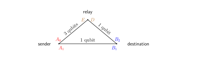
Figure 4: A graphical representation for the noiseless relay channel in Example 1. Alice can transmit three qubits to the relay, from $A_{0}$ to $E$, and a single qubit to Bob, from $A_{1}$ to $B_{1}$. The relay can send a single qubit to Bob, from $D$ to $B_{2}$.

VI Summary and Discussion

We consider the fully quantum relay channel $\mathcal{N}_{AD\to BE}$, where Alice transmits $A$, the relay transmits $D$, Bob receives $B$, and the relay receives $E$. When there are multiple rounds of communication, synchronization is important. Suppose that the operation is governed by a central clock that ticks $n$ times. Between the clock ticks $i-1$ and $i$, the sender and the relay transmit the channel inputs $A_{i}$ and $D_{i}$, respectively. See Figure 2. Then, at clock tick $i$, the relay and destination receivers receive the channel outputs $E_{i}$ and $B_{i}$, respectively. This requires a small delay before reception to ensure causality. The relay is only required to assist the transmission of information to Bob, and does not necessarily decode any information (see Remark 1). The classical channel model was originally introduced by van der Meulen [31] as a building block for multihop networks [32]. Here, we consider the quantum counterpart.

Our coding definitions in Section III are more involved than in the classical setting. Since the channel is fully quantum, we need to account for the post-operation state at the relay in each time instance (see Remark 2). That is, the relay encoding at time $i$ affects the state of $E_{i-1}$, as well as the previous outputs. The system $\bar{E}^{i-1}$ in Section III can thus be viewed as a “leftover" of the relay encoding at time $i$. This leftover can be used in subsequent steps, at time $j>i$. For example, if the relay performs a sequence of measurements, then at time $i$, the relay applies a quantum instrument such that $\bar{E}^{i-1}$ is the post-measurement system, while $D_{i}$ stores the measurement outcome. In the classical setting, $\bar{E}^{i-1}$ is simply a copy of the previously received observations at the relay.

We establish three bounds that are based on different coding strategies, i.e., partial decode-forward, measure-forward, and assist-forward. Using the partial-decode forward strategy, the relay decodes part of the information, while the other part is decoded without the relay’s help (Section IV-A). Based on the partial-decode forward bound, we determine the capacity for the special class of Hadamard relay channels. We also recover the result by Savov et al. [33] for the special case of a classical-quantum relay channel. Furthermore, we observed that when the relay receives Bob’s entire environment, our results yield a bound that resembles the environment-assisted distillation rate [37, 38].

The formula for the partial decode-forward bound includes three random variables, $X_{0}$, $X_{1}$, and $U$. Intuitively, the auxiliary variables are associated with the information sent by the sender, the information sent by the relay, and the information that is decoded by the relay, respectively (see Remark 3). Taking $U$ to be null, we obtain the direct-transmission lower bound, i.e., the Holevo information (see Remark 4). In the case of an anti-degraded classical-quantum channel, direct transmission is optimal. This capacity result is intuitive, since Bob’s channel is better than the relay’s in this trivial case (see Remark 5). On the other hand, taking $U=X_{0}$ implies that the relay decodes the entire message, which corresponds to a full decode-forward strategy (see (18)). This turns out to be optimal for Hadamard relay channels, as established in Thoerem 3.

In the measure-forward coding scheme, the relay does not decode information at all (Section IV-B). Instead, the relay performs a sequence of measurements, and then sends a compressed representation of the measurement outcome. This generalizes the classical compress-forward bound [49]. We interpret the formula as follows. The encoder and the relay prepare their input states using input ensembles that are indexed by $X_{0}$ and $X_{1}$, respectively. The relay receives $E$ and performs a measurement, which yields $Y_{1}$ as an outcome. The measurement outcome is then compressed and encoded by $Z_{1}$. Bob receives the output $B$. Roughly speaking, the number of information bits that are obtained from the measurement compression operation is $nI(Z_{1};Y_{1}|X_{1}B)_{\omega}$, while the number of information bits that the relay can send through the channel to Bob is below $nI(X_{1};B)_{\rho}$. This limitation is reflected through the maximization constraint, $I(Z_{1};Y_{1}|X_{1}B)_{\omega}\leq I(X_{1};B)_{\rho}$ (see Remark 6).

At last, we consider quantum relay channels with orthogonal receiver components (Section IV-C). In this case, Bob’s output has two components $B_{1}$ and $B_{2}$, and the quantum relay channel is a product of two channels, a broadcast channel from the sender to the relay and the receiver component $B_{1}$, and a direct channel from the relay to the receiver component $B_{2}$. The relay channel is referred to as having orthogonal receiver components due to this decoupling (see Remark 7). The assist-forward bound is based on a new approach, whereby the transmitter sends the message to the relay and simultaneously generates entanglement assistance between the relay and the destination receiver. Subsequently, the relay can transmit the message to the destination receiver with rate-limited entanglement assistance. We interpret the formula for the assist-forward bound as follows. The input to the broadcast channel is chosen from an ensemble $\{\theta^{x_{1}}\}$. Alice can send the message to the relay in this manner at rate $R<I(X_{1};E)_{\theta}$. Alice also generates entangled pairs, $G_{0}^{n}$ and $G_{1}^{n}$. She simultaneously uses the broadcast channel to distribute the entanglement between Bob and the relay, respectively. The entanglement rate is roughly $Q=\min\left\{I(G_{0}\rangle B_{1}X_{1})_{\theta}\,,\;I(G_{1}\rangle EX_{1})_{\theta}\right\}$. In the subsequent block, the relay and Bob perform an entanglement-assisted communication protocol, using the entanglement resources that were generated in the previous block. This requires both $R<I(X_{2}G_{2};B_{2})_{\zeta}$ and $R<I(X_{2};B_{2})_{\zeta}+I(G_{2}\rangle B_{2}X_{2})_{\zeta}+Q$, based on Shor’s result [53] on rate-limited entanglement assistance (see Remark 8).

Section V demonstrate our results through two examples. The first is a trivial example that represents a wired network, where the links are noiseless. We observe that both the partial decode-forward and assist-forward are capacity achieving in this case. Furthermore, we our measure-forward result in order to compute an achievable rate for a depolarizing relay channel with orthogonal receiver components.

Attenuation in optical fibers poses a significant challenge for long-distance quantum communication protocols. This limitation affects current applications such as quantum key distribution [57], and future development of the quantum Internet [58] and quantum networks more broadly [12]. Quantum repeaters have emerged as a promising solution by acting as a relay of quantum information [43]. Here, we addressed the classical task of sending messages through the channel. In order to distribute entanglement and send quantum information, the quantum relay would need to operate as a quantum repeater [43]. In the model’s simplest form, the sender employs quantum communication to the relay (repeater) in order to generate an EPR pair $\ket{\Phi_{AE}}$ between Alice and the relay. At the same time, the relay generates an EPR pair $\ket{\Phi_{DB}}$ with the destination receiver. Then, the repeater can perform a Bell measurement on $E,D$, thus swapping the entanglement such that $A$ and $B$ are now entangled. Pereg et al. [25] provided an information-theoretic perspective on quantum repeaters through the task of quantum subspace transmission via a primitive relay channel, with a noiseless qubit pipe from the relay to the destination receiver. The general case remains unsolved.

Appendix A Information Theoretic Tools

Our analysis builds on the quantum method of types. The basic definitions and lemmas that are used in the analysis are given below.

A-A Typical Projectors

We begin with the classical typical set. The type of a classical sequence $x^{n}\in\mathcal{X}^{n}$ is defined as the empirical distribution $\hat{P}_{x^{n}}(a)=N(a|x^{n})/n$ for $a\in\mathcal{X}$, where $N(a|x^{n})$ is the number of occurrences of the letter $a\in\mathcal{X}$ in the sequence $x^{n}$. Let $\delta>0$. The $\delta$-typical set with respect to a probability distribution $p_{X}$ is defined as the following set of sequences,

$$T_{\delta}^{(n)}(p_{X})=\left\{x^{n}\in\mathcal{X}^{n}\,:\;\absolutevalue{p_{X}(a)-\hat{P}_{x^{n}}(a)}\leq\delta p_{X}(a)\,,\;\text{for all $a\in\mathcal{X}$}\right\}\,.$$ (45)

If $p_{X}$ is a type on $\mathcal{X}^{n}$, then $\mathcal{T}^{(n)}(p_{X})$ denotes the corresponding type class, i.e.,

$$\mathcal{T}^{(n)}(p_{X})=\left\{x^{n}\in\mathcal{X}^{n}\,:\;\hat{P}_{x^{n}}(a)=p_{X}(a)\,,\;\text{for all $a\in\mathcal{X}$}\right\}\,.$$ (46)

For a pair of sequences $x^{n}$ and $y^{n}$, we give similar definitions in terms of the joint type $\hat{P}_{x^{n},y^{n}}(a,b)=N(a,b|x^{n},y^{n})/n$ for $a\in\mathcal{X}$, $b\in\mathcal{Y}$, where $N(a,b|x^{n},y^{n})$ is the number of occurrences of the symbol pair $(a,b)$ in the sequence $(x_{i},y_{i})_{i=1}^{n}$.

We move to the quantum method of types. Consider an ensemble $\{p_{X}(x),\ket{x}\}_{x\in\mathcal{X}}$, with an average density operator,

$$\rho=\sum_{x\in\mathcal{X}}p_{X}(x)\outerproduct{x}{x}\,.$$ (47)

The $\delta$-typical projector $\Pi_{\delta}^{(n)}(\rho)$ is an operator that projects onto the subspace spanned by vectors $\ket{x^{n}}$ that correspond to $\delta$-typical sequences. Specifically,

$$\Pi_{\delta}^{(n)}(\rho)\equiv\sum_{x^{n}\in T_{\delta}^{(n)}(p_{X})}\outerproduct{x^{n}}{x^{n}}$$ (48)

with $\ket{x^{n}}=\bigotimes_{i=1}^{n}\ket{x_{i}}$. Let $0<\delta<\nu_{X}$, where $\nu_{X}\equiv\min\{p_{X}(a)\,:\;p_{X}(a)>0\}$. Based on the classical typicality properties [30, Th. 1.1],

$$\mathrm{Tr}\left\{\Pi_{\delta}^{(n)}(\rho)\rho^{\otimes n}\right\} \geq 1-\varepsilon_{\delta}(n)\,,\;$$ (49)

$$\mathrm{Tr}\left\{\Pi_{\delta}^{(n)}(\rho)\right\} \leq 2^{n(1+\delta)H(\rho)}\,,\;$$ (50)

$$\Pi_{\delta}^{(n)}(\rho)\cdot\rho^{\otimes n}\cdot\Pi_{\delta}^{(n)}(\rho) \leq 2^{-n(1-\delta)H(\rho)}\cdot\Pi_{\delta}^{(n)}(\rho)$$ (51)

where $\varepsilon_{\delta}(n)=2d_{A}e^{-n\nu_{X}\delta^{2}}$.

We will also need conditional typicality. Consider an ensemble $\{p_{X}(x),\rho_{x}\}_{x\in\mathcal{X}}$ in $\mathfrak{D}(\mathcal{H}_{B})$, with an average classical-quantum state

$$\omega_{XB}=\sum_{a\in\mathcal{X}}p_{X}(a)\outerproduct{a}{a}_{X}\otimes\rho_{a}\,.$$ (52)

Each state in the ensemble has a spectral decomposition $\rho_{a}=\sum_{b\in\mathcal{Y}}p_{Y|X}(b|a)\outerproduct{\psi_{a,b}}{\psi_{a,b}}$, for $a\in\mathcal{X}$. Given a fixed sequence $x^{n}\in\mathcal{X}^{n}$, divide the index set $[1:n]$ into the subsets $I_{n}(a)=\{i:x_{i}=a\}$, $a\in\mathcal{X}$. The conditional $\delta$-typical projector $\Pi_{\delta}^{(n)}(\omega|x^{n})$ is defined such that for every $a\in\mathcal{X}$, we apply the $\delta$-typical projector with respect to $\rho_{a}$ on the systems $\{B_{i}\,:\;x_{i}=a\}$. Specifically,

$$\Pi_{\delta}^{(n)}(\omega_{XB}|x^{n})\equiv\bigotimes_{a\in\mathcal{X}}\Pi_{\delta}^{(N(a|x^{n}))}(\rho_{a})\,.$$ (53)

Fix $0<\delta_{1}<\delta<\nu_{XY}$ and $x^{n}\in T_{\delta_{1}}(p_{X})$. Based on the classical typicality properties [30, Th. 1.2],

$$\mathrm{Tr}\left\{\Pi_{\delta}^{(n)}(\omega_{XB}|x^{n})\rho_{x^{n}}\right\} \geq 1-\varepsilon_{\delta_{1},\delta}(n)\,,\;$$ (54)

$$\mathrm{Tr}\left\{\Pi_{\delta}^{(n)}(\omega_{XB}|x^{n})\right\} \leq 2^{n(1+\delta)H(B|X)_{\omega}}\,,\;$$ (55)

$$\Pi_{\delta}^{(n)}(\omega_{XB}|x^{n})\cdot\rho_{x^{n}}\cdot\Pi_{\delta}^{(n)}(\omega_{XB}|x^{n}) \leq 2^{-n(1-\delta_{1})H(B|X)_{\omega}}\cdot\Pi_{\delta}^{(n)}(\omega|x^{n})$$ (56)

where $\varepsilon_{\delta_{1},\delta}(n)=1-\left[1-\varepsilon_{\delta}\left(n(1-\delta_{1})\nu_{X})\right)\right]^{d_{A}}$ and $\rho_{x^{n}}\equiv\bigotimes_{i=1}^{n}\rho_{x_{i}}$. Furthermore,

$$\mathrm{Tr}(\Pi^{\delta}(\omega_{B})\rho_{x^{n}})\geq 1-\varepsilon_{\delta_{1},\delta}(n)$$ (57)

(see [56, Property 15.2.7]).

In a random coding scheme, it is often useful to limit the codewords to the $\delta$-typical set. Given a probability distribution $p_{X}$ on $\mathcal{X}$, denote the $n$-fold product by $p^{n}_{X}$, i.e.,

$$p^{n}_{X}(x^{n})\equiv\prod_{i=1}^{n}p_{X}(x_{i})\,,\,\text{ for $x^{n}\in\mathcal{X}^{n}$.}$$ (58)

Then, define a distribution $\bar{p}_{X^{n}}$ by

$$\bar{p}_{X^{n}}(x^{n})=\begin{cases}p_{X}^{n}(x^{n})/\sum\limits_{x^{\prime n}\in T_{\delta}(p_{X})}p_{X}^{n}(x^{\prime n})&\text{if $x^{n}\in T_{\delta}(p_{X})$}\\ 0&\text{if $x^{n}\notin T_{\delta}(p_{X})$}\end{cases}$$ (59)

and let

$$\bar{\rho}_{B^{n}}=\sum_{x^{n}\in T_{\delta}^{(n)}(p_{X})}\bar{p}_{X^{n}}(x^{n})\rho_{x^{n}}$$ (60)

Then, we have the following properties

$$\sum_{x^{n}\in\mathcal{X}^{n}}\absolutevalue{\bar{p}_{X^{n}}(x^{n})-p_{X}^{n}(x^{n})} \leq 2\varepsilon_{\delta}(n)\,,$$ (61)

$$\Pi_{\delta}^{(n)}(\omega_{B})\cdot\bar{\rho}_{B^{n}}\cdot\Pi_{\delta}^{(n)}(\omega_{B}) \leq 2^{-n\left((1-\delta)H(B)_{\omega}-\bar{\varepsilon}_{\delta}(n)\right)}\Pi_{\delta}^{(n)}(\omega_{B})\,.$$ (62)

where $\bar{\varepsilon}_{\delta}(n)=-\frac{1}{n}\log[1-\varepsilon_{\delta}(n)]$ (see [56, Ex. 20.3.2]). Notice that $\varepsilon_{\delta}(n)$, $\bar{\varepsilon}_{\delta}(n)$, $\varepsilon_{\delta_{1},\delta}(n)$ all tend to zero as $n\to\infty$. A joint distribution $\bar{p}_{X^{n}Y^{n}}$ is defined in the same manner, with respect to the joint typical set.

A-B Quantum Packing and Gentle Measurement Lemmas

The quantum packing lemma is a useful tool in achievability proofs. Consider the following one-shot communication setting. Suppose that Alice has a classical codebook that consists of $\mathsf{M}$ codewords. Given a message $m\in[1:\mathsf{M}]$, she sends a codeword $x(m)$ through a classical-quantum channel, producing an output state $\rho_{x(m)}$ at the receiver. The quantum packing lemma provides a decoding measurement in order for Bob to recover $m$, by using a random codebook. The proof is based on the square-root measurement [52, 59].

Lemma 6 (Quantum Packing Lemma [60]).

Consider an ensemble, $\{p_{X}(x),\rho_{x}\}_{x\in\mathcal{X}}$, with an average state,

$$\rho=\sum_{x\in\mathcal{X}}p_{X}(x)\rho_{x}\,.$$ (63)

Furthermore, suppose that there exist a code projector $\Pi$ and codeword projectors $\Pi_{x}$, $x\in\mathcal{X}$, that satisfy the following conditions:

$$\mathrm{Tr}(\Pi\rho_{x}) \geq\,1-\varepsilon$$ (64)

$$\mathrm{Tr}(\Pi_{x}\rho_{x}) \geq\,1-\varepsilon$$ (65)

$$\mathrm{Tr}(\Pi_{x}) \leq\,2^{\mathsf{h}}$$ (66)

$$\Pi\rho\Pi \leq\,2^{-\mathsf{H}}\Omega$$ (67)

for all $x\in\mathcal{X}$ and some $\varepsilon\in(0,1)$, $0<\mathsf{h}<\mathsf{H}$. Let $\mathscr{A}=\{X(m)\}_{m\in[1:\mathsf{M}]}$, be a random codebook of size $\mathsf{M}$, where the codewords are drawn independently at random, according to $p_{X}$. Then, there exists a decoding POVM $\{\Lambda_{m}\}_{m\in[1:\mathsf{M}]}$ such that the expected probability of error satisfies

$$\mathbb{E}_{\mathscr{A}}\left[1-\frac{1}{\mathsf{M}}\sum_{m=1}^{\mathsf{M}}\mathrm{Tr}\left\{\Lambda_{m}\cdot\rho_{X(m)}\right\}\right]\leq 2(\varepsilon+2\sqrt{\varepsilon})+4\mathsf{M}\cdot 2^{-(\mathsf{H}-\mathsf{h})}$$ (68)

where the expectation is with respect to the random codebook, $\mathscr{A}=\{X(m)\}$.

The gentle measurement lemma is useful in our analysis, since it guarantees that we can perform multiple measurements such that the state of the system remains almost the same after each measurement (see also [41]).

Lemma 7 (Gentle Measurement Lemma [54, 61]).

Let $\rho$ be a density operator. Suppose that $\Lambda$ is a measurement operator such that $0\leq\Lambda\leq\mathbbm{1}$. If

$$\mathrm{Tr}(\Lambda\rho)\geq 1-\delta$$ (69)

for some $0\leq\varepsilon\leq 1$, then the post-measurement state $\tilde{\rho}\equiv\frac{\sqrt{\Lambda}\rho\sqrt{\Lambda}}{\mathrm{Tr}(\Lambda\rho)}$ is $2\sqrt{\delta}$-close to the original state in trace distance, i.e.

$$\norm{\rho-\tilde{\rho}}_{1}\leq 2\sqrt{\delta}\,.$$ (70)

In our analysis, we will establish the conditions of the gentle measurement lemma based on the property (68), arising from the quantum packing lemma.

Appendix B Proof of Theorem 1 (Partial Decode-Forward Strategy)

Consider a quantum relay channel $\mathcal{N}_{AD\to BE}$. The proof extends the classical scheme of partial decode-forward coding, along with observations from a previous work by the author [41].

We show that for every $\varepsilon_{0},\delta_{0}>0$, there exists a $(2^{n(R-\delta_{0})},n,\varepsilon_{0})$ code for the quantum relay channel $\mathcal{N}_{DA\to BE}$, provided that $R<\mathsf{R}_{\text{PD-F}}(\mathcal{N})$. To prove achievability, we extend the classical block Markov coding to the quantum setting, and then apply the quantum packing lemma and the classical covering lemma. We use the gentle measurement lemma [54], which guarantees that multiple decoding measurements can be performed without “destroying" the output state.

Fix a given input ensemble, $\{p_{U}(u)p_{X_{0}X_{1}|U}(x_{0},x_{1}|u),\theta_{A}^{x_{0}}\otimes\zeta_{D}^{x_{1}}\}$. Denote the output states by

$$\omega_{BE}^{x_{0},x_{1}} \equiv\mathcal{N}_{AD\to BE}(\theta_{A}^{x_{0}}\otimes\zeta_{D}^{x_{1}})\,,$$ (71)

and the average states,

$$\omega_{AD}^{u,x_{0}} \equiv\theta_{A}^{x_{0}}\otimes\sum_{x_{1}\in\mathcal{X}_{1}}p_{X_{1}|X_{0}U}(x_{1}|x_{0},u)\zeta_{D}^{x_{1}}\,,\;\omega_{BE}^{u,x_{0}}\equiv\mathcal{N}_{AD\to BE}(\omega_{AD}^{u,x_{0}})\,,$$ (72)

$$\omega_{AD}^{u,x_{1}} \equiv\sum_{x_{0}\in\mathcal{X}_{0}}p_{X_{0}|X_{1}U}(x_{0}|x_{1},u)\theta_{A}^{x_{0}}\otimes\zeta_{D}^{x_{1}}\,,\;\omega_{BE}^{u,x_{1}}\equiv\mathcal{N}_{AD\to BE}(\omega_{AD}^{u,x_{1}})\,,$$ (73)

$$\omega_{BE} \equiv\sum_{u\in\mathcal{U}}p_{U}(u)\sum_{x_{0}\in\mathcal{X}_{0}}\sum_{x_{1}\in\mathcal{X}_{1}}p_{X_{0}X_{1}|U}(x_{0},x_{1}|u)\omega_{BE}^{x_{0},x_{1}}\,,$$ (74)

for $(u,x_{0},x_{1})\in\mathcal{U}\times\mathcal{X}_{0}\times\mathcal{X}_{1}$.

Recall that the relay encodes in a strictly-causal manner. Specifically, the relay has access to the sequence of previously received systems, $E_{i-1},\bar{E}^{i-2}$, from the past. We use $T$ transmission blocks, where each block consists of $n$ input systems. In particular, the relay has access to the systems from the previous blocks. In effect, the $j^{\text{th}}$ transmission block of the relay encodes part of the message $m_{j-1}\in[1:2^{nR}]$ from the previous block.

First, we use rate splitting. Let every message $m_{j}$, $j\in[1:T-1]$, comprise two independent components $m_{j}^{\prime}$ and $m_{j}^{\prime\prime}$, where $m_{j}^{\prime}\in[1:2^{nR^{\prime}}]$ and $m_{j}^{\prime\prime}\in[1:2^{nR^{\prime\prime}}]$, such that $R=R^{\prime}+R^{\prime\prime}$. The coding scheme is referred to as a “partial decode-forward" strategy, since the relay decodes the first component alone.

B-A Code Construction

The code construction, encoding and decoding procedures are described below. We illustrate the code structure in Figure 5.

Block	$1$	$2$	$\cdots$	$T-1$	$T$
$U$	$u^{n}(m_{1}^{\prime}|1)$	$u^{n}(m_{2}^{\prime}|m_{1}^{\prime})$	$\cdots$	$u^{n}(m_{T-1}^{\prime}|m_{T-2}^{\prime}))$	$u^{n}(1|m_{T-1}^{\prime}))$
$A$	$x_{0}^{n}(m_{1}^{\prime},m_{1}^{\prime\prime}|1)$	$x_{0}^{n}(m_{2}^{\prime},m_{2}^{\prime\prime}|m_{1}^{\prime})$	$\cdots$	$x_{0}^{n}(m_{T-1}^{\prime},m_{T-1}^{\prime\prime}|m_{T-2}^{\prime})$	$x_{0}^{n}(1,m_{1}^{\prime\prime}|m_{T-1}^{\prime})$
$E$	$\tilde{m}_{1}^{\prime}\rightarrow$	$\tilde{m}_{2}^{\prime}\rightarrow$	$\cdots$	$\tilde{m}_{T-1}^{\prime}\rightarrow$	$\emptyset$
$D$	$x_{1}^{n}(1)$	$x_{1}^{n}(\tilde{m}_{1}^{\prime})$	$\cdots$	$x_{1}^{n}(\tilde{m}_{T-2}^{\prime})$	$x_{1}^{n}(\tilde{m}_{T-1}^{\prime})$
$B$	$\emptyset$	$\leftarrow\hat{m}_{1}^{\prime}$	$\cdots$	$\leftarrow\hat{m}_{T-2}^{\prime}$	$\leftarrow\hat{m}_{T-1}^{\prime}$
	$\hat{m}_{1}^{\prime\prime}$	$\hat{m}_{2}^{\prime\prime}$	$\cdots$	$\hat{m}_{T-1}^{\prime\prime}$	$\emptyset$

Figure 5: Partial decode-forward strategy. The block index $j\in[1:T]$ is indicated at the top. In the following rows, we have the corresponding elements: (1) auxiliary sequences; (2) codewords of Alice; (3) relay estimates; (4) relay codewords; (5), (6) estimated messages at the destination receiver. The arrows in the third row indicate that the relay measures and encodes forward with respect to the block index, while the arrows in the fifth row indicate that Bob decodes backwards.

B-A1 Classical Codebook Construction

For every $j\in[1:T]$, generate a classical codebook $\mathscr{B}(j)$ as follows. Select $2\cdot 2^{nR^{\prime}}$ independent sequences $u^{n}(m_{j}^{\prime}|m_{j-1}^{\prime})$, for $m_{j}^{\prime},m_{j-1}^{\prime}\in[1:2^{nR^{\prime}}]$, according to $\bar{p}_{U^{n}}$ (see the first row in Figure 5). Then, for every given $u^{n}(m_{j}^{\prime}|m_{j-1}^{\prime})$, select conditionally independent $(x_{0}^{n}(m_{j}^{\prime},m_{j}^{\prime\prime}|m_{j-1}^{\prime}),x_{1}^{n}(m_{j-1}^{\prime}))$, for $m_{j}^{\prime\prime}\in[1:2^{nR^{\prime\prime}}]$, according to $\bar{p}_{X_{0}^{n}X_{1}^{n}|U^{n}}(\cdot,\cdot|u^{n})$, conditioned on $u^{n}\equiv u^{n}(m_{j}^{\prime}|m_{j-1}^{\prime})$.

B-A2 Encoding

Set $m_{0}^{\prime}=m_{T}^{\prime}=m_{T}^{\prime\prime}\equiv 1$. Given the message sequence $(m_{j}^{\prime},m_{j}^{\prime\prime})_{j\in[1:T]}$, prepare the input state $\bigotimes_{j=1}^{T}\rho_{A^{n}(j)}$, where

$$\rho_{A^{n}(j)}=\bigotimes_{i=1}^{n}\theta_{A}^{x_{0,i}}\,\text{ for $x_{0}^{n}\equiv x_{0}^{n}(m_{j}^{\prime},m_{j}^{\prime\prime}|m_{j-1}^{\prime})$}\,.$$ (75)

Then, transmit $A^{n}(j)$ in Block $j$, for $j=1,2,\ldots,T$. Hence, we encode in an average rate of $\left(\frac{T-1}{T}\right)R$, which tends to $R$ as $T\to\infty$.

The encoding operation is illustrated in the second row of Figure 5.

B-A3 Relay Encoding

Set $\tilde{m}_{0}^{\prime}\equiv 1$.

1. At the end of Block $j$, find an estimate $\tilde{m}_{j}^{\prime}$ by performing a measurement $\{\Gamma_{m_{j}^{\prime}|x_{1}^{n}}\}_{m_{j}^{\prime}\in[1:2^{nR^{\prime}}]}$ for $x_{1}^{n}\equiv x_{1}^{n}(\tilde{m}_{j-1}^{\prime})$, which will be specified later, on the received systems $E^{n}(j)$, for $j=1,2,\ldots,T-1$.

2. In block $j+1$, prepare the state

   $$\rho_{D^{n}(j+1)}=\bigotimes_{i=1}^{n}\zeta_{D}^{x_{1,i}}\,,\;\text{for $x_{1}^{n}\equiv x_{1}^{n}(\tilde{m}_{j}^{\prime})$}$$ (76)

   using the classical codebook $\mathscr{B}(j+1)$. Then, transmit $D^{n}(j+1)$. The relay’s decoding and encoding operations are illustrated in the third and fourth rows in Figure 5.

This results in the output state $\bigotimes_{j=1}^{T}\rho_{B^{n}(j)E^{n}(j)}$, where

$$\rho_{B^{n}(j)E^{n}(j)}=\bigotimes_{i=1}^{n}\omega_{BE}^{x_{0,i},x_{1,i}}\,,\;$$

for $$x_{0}^{n}\equiv x_{0}^{n}(m_{j}^{\prime},m_{j}^{\prime\prime}|m_{j-1}^{\prime}) x_{1}^{n}\equiv x_{1}^{n}(\tilde{m}_{j}^{\prime})$$ and . (77)

B-A4 Decoding

Bob receives the $T$ output blocks, $B^{n}(1),\ldots,B^{n}(T)$, and decodes as follows.

1. Decoding $(m_{j}^{\prime})_{j\in[1:T]}$ is performed backwards. Set $\hat{m}_{0}^{\prime}=\hat{m}_{T}^{\prime}\equiv 1$. For $j=T-1,T-2,\ldots 1$, find an estimate $\hat{m}_{j}^{\prime}$ by performing a measurement $\{\Delta^{1}_{m_{j}^{\prime}|\hat{m}_{j+1}^{\prime}}\}$, which will be specified later, on the output systems $B^{n}(j+1)$. See the fifth row in Figure 5.

2. Next, we decode $(m_{j}^{\prime\prime})_{j\in[1:T]}$ as follows. For $j=1,2,\ldots T-1$, find an estimate $\hat{m}_{j}^{\prime\prime}$ by performing a second measurement $\{\Delta^{2}_{m_{j}^{\prime\prime}|u^{n},x_{1}^{n}}\}$ for $u^{n}\equiv u^{n}(\hat{m}_{j}^{\prime}|\hat{m}_{j-1}^{\prime\prime})$ and $x_{1}^{n}\equiv x_{1}^{n}(\hat{m}_{j}^{\prime})$ , which will also be specified later, on $B^{n}(j)$. See the last row in Figure 5.

B-B Error Analysis

By symmetry, we may assume without loss of generality that Alice sends the messages $(M_{j}^{\prime},M_{j}^{\prime\prime})=(1,1)$, for $j\in[1:T]$. Consider the error events,

$$\mathscr{E}_{0}(j) =\{\widetilde{M}_{j}^{\prime}\neq 1\}\,,$$ (78)

$$\mathscr{E}_{1}(j) =\{\widehat{M}_{j}^{\prime}\neq 1\}\,,$$ (79)

$$\mathscr{E}_{2}(j) =\{\widehat{M}_{j}^{\prime\prime}\neq 1\}\,.$$ (80)

The event $\mathscr{E}_{0}(j)$ is associated with erroneous decoding by the relay, and $\mathscr{E}_{1}(j)$, $\mathscr{E}_{2}(j)$ by the destination receiver. By the union of events bound, the expected probability of error is bounded by

$$\mathbb{E}P_{e}^{(Tn)}(\mathscr{C}) \leq\sum_{j=1}^{T-1}\Pr({\mathscr{E}_{0}(j)})+\sum_{j=1}^{T-1}\Pr({\mathscr{E}_{1}(j)}|{\mathscr{E}_{0}^{c}(j)\cap\mathscr{E}_{1}^{c}(j+1)})$$

$$+\sum_{j=1}^{T}\Pr({\mathscr{E}_{2}(j)}|{\mathscr{E}_{0}^{c}(j)\cap\mathscr{E}_{1}^{c}(j)\cap\mathscr{E}_{1}^{c}(j-1)})$$ (81)

where the conditioning on $M_{j}^{\prime}=M_{j-1}^{\prime}=M_{j}^{\prime\prime}=1$ is omitted for convenience of notation.

To bound the first sum, we use the quantum packing lemma, Lemma 6. Observe that based on the quantum typicality properties in Section A-A of Appendix A, we have for sufficiently large $n$,

$$\mathrm{Tr}\left[\Pi_{\delta}^{(n)}(\omega_{X_{1}E}|x_{1}^{n})\omega_{E^{n}}^{u^{n},x_{1}^{n}}\right] \geq 1-\delta$$ (82)

$$\mathrm{Tr}\left[\Pi_{\delta}^{(n)}(\omega_{UX_{1}E}|u^{n},x_{1}^{n})\omega_{E^{n}}^{u^{n},x_{1}^{n}}\right] \geq 1-\delta$$ (83)

$$\mathrm{Tr}\left[\Pi_{\delta}^{(n)}(\omega_{UX_{1}E}|u^{n},x_{1}^{n})\right] \leq 2^{n(1+2\delta)H(E|UX_{1})_{\omega}}$$ (84)

$$\Pi_{\delta}^{(n)}(\omega_{X_{1}E}|x_{1}^{n})\omega^{x_{1}^{n}}_{E^{n}}\Pi_{\delta}^{(n)}(\omega_{X_{1}E}|x_{1}^{n}) \leq 2^{-n(1-2\delta)H(E|X_{1})_{\omega}}\Pi_{\delta}^{(n)}(\omega_{E})$$ (85)

for all $(u^{n},x_{1}^{n})\in T^{(n)}_{\delta_{1}}(p_{U}p_{X_{1}|U})$ (see (54)-(57)). Since the codebooks are statistically independent of each other, we have by Lemma 6 that there exists a POVM $\Gamma_{m_{j}^{\prime}|x_{1}^{n}}$ such that $\Pr({\mathscr{E}_{0}(j)})\leq 2^{-n(I(U;E|X_{1})_{\omega}-R^{\prime}-\varepsilon_{1})}$, which tends to zero as $n\rightarrow\infty$, provided that

$$R^{\prime}<I(U;E|X_{1})_{\omega}-\varepsilon_{1}$$ (86)

for $\varepsilon_{1}=\varepsilon_{1}(\delta)\equiv 4\delta\log(d_{E})$.

Moving to the third sum in the RHS of (81), suppose that $\mathscr{E}_{1}^{c}(j)\cap\mathscr{E}_{2}^{c}(j+1)$ occurred. Namely, the relay measured the correct $M_{j}^{\prime}$, and the decoder recovered $M_{j+1}^{\prime}$. Then, by the same packing lemma argument as given above, there exists a POVM $\Delta^{1}_{m_{j}^{\prime}|m_{j+1}^{\prime}}$ such that $\Pr({\mathscr{E}_{2}(j)}|\mathscr{E}_{1}^{c}(j)\cap\mathscr{E}_{2}^{c}(j+1))\leq 2^{-n(I(UX_{1};B)_{\omega}-R^{\prime}-\varepsilon_{2})}$, which tends to zero as $n\rightarrow\infty$ for

$$R^{\prime}<I(UX_{1};B)_{\omega}-3\varepsilon_{2}$$ (87)

where $\varepsilon_{2}=\varepsilon_{2}(\delta)\equiv 4\delta\log(d_{B})$.

Denote the state of the output systems $B^{n}(j)$ in Block $j$, after this measurement, by $\tilde{\rho}_{B^{n}(j)}$. Then, observe that due to the packing lemma inequality (68), the gentle measurement lemma [54, 61], Lemma 7, implies that the post-measurement state is close to the original state in the sense that

$$\frac{1}{2}\norm{\tilde{\rho}_{B^{n}(j)}-\rho_{B^{n}(j)}}_{1}\leq 2^{-n\frac{1}{2}(I(UX_{1};B)_{\omega}-R^{\prime}-\varepsilon_{2})}\leq 2^{-\varepsilon_{2}n}$$ (88)

for sufficiently large $n$ and rates as in (87). Therefore, the distribution of measurement outcomes when $\tilde{\rho}_{B^{n}(j)}$ is measured is roughly the same as if the POVM $\Delta^{1}_{m_{j}^{\prime}|m_{j+1}^{\prime}}$ was never performed. To be precise, the difference between the probability of a measurement outcome $\hat{m}_{j}^{\prime\prime}$ when $\tilde{\rho}_{B^{n}(j)}$ is measured and the probability when $\rho_{B^{n}(j)}$ is measured is bounded by $2^{-\varepsilon_{2}n}$ in absolute value [56, Lemma 9.11]. Furthermore, the $\delta$-typicality properties:

$$\mathrm{Tr}\left[\Pi_{\delta}^{(n)}(\omega_{UX_{1}B}|u^{n},x_{1}^{n})\omega_{B^{n}}^{u^{n},x_{0}^{n},x_{1}^{n}}\right] \geq 1-\delta$$ (89)

$$\mathrm{Tr}\left[\Pi_{\delta}^{(n)}(\rho_{UX_{0}X_{1}B}|u^{n},x_{0}^{n},x_{1}^{n})\omega_{B^{n}}^{u^{n},x_{0}^{n},x_{1}^{n}}\right] \geq 1-\delta$$ (90)

$$\mathrm{Tr}\left[\Pi_{\delta}^{(n)}(\omega_{UX_{0}X_{1}B}|u^{n},x_{0}^{n},x_{1}^{n})\right] \leq 2^{n(1+2\delta)(H(B|UX_{0}X_{1})_{\omega}}$$ (91)

$$\Pi_{\delta}^{(n)}(\omega_{UX_{1}B}|u^{n},x_{1}^{n})\omega^{u^{n},x_{1}^{n}}_{B^{n}}\Pi_{\delta}^{(n)}(\omega_{UX_{1}B}|u^{n},x_{1}^{n}) \leq 2^{-n(1-2\delta)H(B|UX_{1})_{\omega}}\Pi_{\delta}^{(n)}(\omega_{UX_{1}B}|u^{n},x_{1}^{n})$$ (92)

imply a POVM $\Delta^{2}_{m_{j}^{\prime\prime}|u^{n},x_{1}^{n}}$ such that

$$\Pr{\mathscr{E}_{3}(j+1)}|{\mathscr{E}_{1}^{c}(j)\cap\mathscr{E}_{2}^{c}(j)\cap\mathscr{E}_{2}^{c}(j-1)} \leq 2^{-n(I(X_{0};B|UX_{1})_{\rho}-R^{\prime\prime}-\varepsilon_{2})}\,,$$ (93)

which tends to zero if

$$R^{\prime\prime}<I(X_{0};B|UX_{1})_{\rho}-\varepsilon_{2}\,.$$ (94)

This completes the proof of the partial decode-forward lower bound. ∎

Appendix C Proof of Theorem 3 (Hadamard Relay Channel)

We prove the capacity theorem for the Hadamard relay channel $\mathcal{N}_{AD\to BY_{1}}^{\text{H}}$, where the relay receives a classical observation $Y_{1}$. Achievability immediately follows from Theorem 1, by taking $U=X_{0}$ in (15). As explained in Remark 4, such a rate can be achieved using a full dicode-forward strategy, where the relay decodes the entire information. That is, we set $R^{\prime\prime}=0$ and thus $R=R^{\prime}$ in the proof of Theorem 1 in Appendix B.

Consider the converse part. Suppose that Alice selects a message $m$ uniformly at random, stores $m$ in a classical register $M$, and then prepares an input state $\rho^{(m)}_{A^{n}}$. At time $i$, the relay performs an encoding channel, mapping $Y_{1}^{i-1}$ to $D_{i}$, This results in a joint state $\rho_{Y_{1}^{i-1}D_{i}A_{i}B^{i-1}}^{(m)}$. Next, the relay receives $Y_{1,i}$ in the state

$$\rho_{MB_{i}Y_{1,i}B^{i-1}Y_{1}^{i-1}} =\frac{1}{2^{nR}}\sum_{m=1}^{2^{nR}}\outerproduct{m}{m}_{M}\otimes(\mathcal{N}^{\text{H}}_{AD\to BY_{1}}\otimes\mathrm{id}_{B^{i-1}Y_{1}^{i-1}})(\rho_{A_{i}D_{i}B^{i-1}Y_{1}^{i-1}}^{(m)})\,,$$ (95)

for $i=1,2,\ldots,n$. Bob receives the channel output systems $B^{n}$, performs a measurement, and obtains an estimate $\widehat{M}$ for Alice’s message.

Consider a sequence of codes $(\mathcal{F}_{n},\Gamma_{n},\Delta_{n})$ such that the average probability of error tends to zero. As usual, we observe that Fano’s inequality [62] implies $H(M|\widehat{M})\leq n\varepsilon_{n}$ and thus

$$nR \leq I(M;\widehat{M})+n\varepsilon_{n}$$

$$\leq I(M;B^{n})_{\rho}+n\varepsilon_{n}$$ (96)

based on the data processing inequality for the quantum mutual information, where $\varepsilon_{n}$ tends to zero as $n\rightarrow\infty$.

Now, we show the following bounds:

$$I(M;B^{n})_{\rho}\leq\sum_{i=1}^{n}I(MY_{1}^{i-1};B_{i})_{\rho}\,,$$ (97a)

and

$$I(M;B^{n})_{\rho}\leq\sum_{i=1}^{n}I(M;Y_{1,i}|Y_{1}^{i-1})_{\rho}\,.$$ (97b)

We begin with the first bound. By the chain rule,

$$I(M;B^{n})_{\rho} =\sum_{i=1}^{n}I(M;B_{i}|B^{i-1})_{\rho}$$

$$\leq\sum_{i=1}^{n}I(MB^{i-1};B_{i})_{\rho}\,.$$ (98)

Recall that the Hadamard relay channel is degraded, i.e., $\mathcal{L}_{DA\to B}=\mathcal{P}_{Y_{1}\to B}\circ\mathcal{M}_{DA\to Y_{1}}$. Therefore,

$$I(MB^{i-1};B_{i})_{\rho}\leq I(MY_{1}^{i-1};B_{i})_{\rho}$$ (99)

by the data processing inequality. The first bound, (97a), now follows from (98)-(99).

Similarly,

$$I(M;B^{n})_{\rho} \leq I(M;Y_{1}^{n})_{\rho}$$

$$=\sum_{i=1}^{n}I(M;Y_{1,i}|Y_{1}^{i-1})_{\rho}\,,$$ (100)

hence the second bound, (97b), holds as well.

Together with (96), this implies

$$R-\varepsilon_{n}\leq\min\left\{\frac{1}{n}\sum_{i=1}^{n}I(X_{0,i}X_{1,i};B_{i})_{\rho}\,,\;\frac{1}{n}\sum_{i=1}^{n}I(X_{0,i};Y_{1,i}|X_{1,i})_{\rho}\right\}$$ (101)

where we have defined

$$X_{0,i}\equiv M\,,\;X_{1,i}\equiv Y_{1}^{i-1}\,.$$ (102)

Let $J$ to be a uniformly distributed random variable, on $\{1,\ldots,n\}$, which has no correlation with the message. Then, we may rewrite (101) as

$$R-\varepsilon_{n}\leq\min\left\{I(X_{0,J}X_{1,J};B_{J}|J)_{\rho}\,,\;I(X_{0,J};Y_{1,J}|X_{1,J}J)_{\rho}\right\}$$ (103)

with $\rho_{JX_{0,J}B_{J}Y_{1,J}B^{J-1}X_{1,J}}=\frac{1}{n}\sum_{i=1}^{n}\outerproduct{i}{i}_{J}\otimes\rho_{X_{0,i}B_{i}Y_{1,i}B^{i-1}X_{1,i}}$. Hence,

$$R-\varepsilon_{n}\leq\min\left\{I(X_{0}X_{1};B)_{\rho}\,,\;I(X_{0};Y_{1}|X_{1})_{\rho}\right\}$$ (104)

for $X_{0}\equiv(J,X_{0,J})$, $X_{1}\equiv X_{1,J}$, and thus $B\equiv B_{J}$ and $Y_{1}\equiv Y_{1,J}$. This completes the proof of Theorem 3. ∎

Appendix D Proof of Theorem 4 (Measure-Forward Strategy)

Consider a quantum relay channel $\mathcal{N}_{AD\to BE}$. The proof extends the classical scheme of compress-forward coding, along with observations from a previous work by the author [41].

We show that for every $\varepsilon_{0},\delta_{0}>0$, there exists a $(2^{n(R-\delta_{0})},n,\varepsilon_{0})$ code for the quantum relay channel $\mathcal{N}_{AD\to BE}$, provided that $R<\mathsf{R}_{\text{M-F}}(\mathcal{N})$. To prove achievability, we extend the classical block Markov coding to the quantum setting, and then apply the quantum packing lemma and the classical covering lemma. We use the gentle measurement lemma [54], which guarantees that multiple decoding measurements can be performed without “destroying" the output state.

Fix a given input ensemble, $\{p_{X_{0}}(x_{0})p_{X_{1}}(x_{1}),\theta_{A}^{x_{0}}\otimes\zeta_{D}^{x_{1}}\}$, a POVM $\{\Gamma_{y_{1}}\}$ on $\mathcal{H}_{E}$, and a classical channel $p_{Z_{1}|X_{1}Y_{1}}$. Denote the output states before the relay measurement by

$$\omega^{x_{0},x_{1}}_{BE} =\mathcal{N}_{AD\rightarrow BE}(\theta^{x_{0}}_{A}\otimes\zeta^{x_{1}}_{D})\,.$$ (105)

Upon measurement, the outcome $Y_{1}$ is distributed according to

$$p_{Y_{1}|X_{0},X_{1}}(y_{1}|x_{0},x_{1})=\mathrm{Tr}(\Gamma_{y_{1}}\omega_{E}^{(x_{0},x_{1})})\,.$$ (106)

This induces the joint distribution

$$p_{X_{0}X_{1}Y_{1}Z_{1}}(x_{0},x_{1},y_{1},z_{1})=p_{X_{0}}(x_{0})p_{X_{1}}(x_{1})p_{Y_{1}|X_{0},X_{1}}(y_{1}|x_{0},x_{1})p_{Z_{1}|X_{1}Y_{1}}(z_{1}|x_{1},y_{1})$$ (107)

for $(x_{0},x_{1},y_{1},z_{1})\in\mathcal{X}_{0}\times\mathcal{X}_{1}\times\mathcal{Y}_{1}\times\mathcal{Z}_{1}$. Furthemore, consider the average states,

$$\omega_{AD}^{x_{1}} \equiv\left(\sum_{x_{0}\in\mathcal{X}_{0}}p_{X_{0}}(x_{0})\theta_{A}^{x_{0}}\right)\otimes\zeta_{D}^{x_{1}}\,,\;\omega_{BE}^{x_{1}}=\mathcal{N}_{AD\to BE}(\omega_{AD}^{x_{1}})\,,$$ (108)

$$\omega_{AD}^{x_{0}} \equiv\theta^{x_{0}}_{A}\otimes\left(\sum_{x_{1}\in\mathcal{X}_{1}}p_{X_{1}}(x_{1})\zeta_{D}^{x_{1}}\right)\,,\;\omega_{BE}^{x_{0}}=\mathcal{N}_{AD\to BE}(\omega_{AD}^{x_{0}})\,,$$ (109)

$$\omega_{AD} \equiv\left(\sum_{x_{0}\in\mathcal{X}_{0}}p_{X_{0}}(x_{0})\theta_{A}^{x_{0}}\right)\otimes\left(\sum_{x_{1}\in\mathcal{X}_{1}}p_{X_{1}}(x_{1})\zeta_{D}^{x_{1}}\right)\,,\;\omega_{BE}\equiv\mathcal{N}_{AD\to BE}(\omega_{AD})$$ (110)

and

$$\omega_{BY_{1}Z_{1}}^{x_{0},x_{1}}=\sum_{y_{1}\in\mathcal{Y}_{1}}\sum_{z_{1}\in\mathcal{Z}_{1}}p_{Y_{1}Z_{1}|X_{0}X_{1}}(y_{1},z_{1}|x_{0},x_{1})\omega_{B}^{x_{0},x_{1}}\otimes\outerproduct{y_{1}}{y_{1}}\otimes\outerproduct{z_{1}}{z_{1}}\,.$$ (111)

We use $T$ transmission blocks, where each block consists of $n$ input systems. In particular, the relay has access to the systems from the previous blocks.

D-A Code Construction

The code construction, encoding and decoding procedures are described below.

Block	$1$	$2$	$\cdots$	$T-1$	$T$
$A$	$x_{0}^{n}(m_{1})$	$x_{0}^{n}(m_{2})$	$\cdots$	$x_{0}^{n}(m_{T-1})$	$x_{0}^{n}(1)$
$E$	$\ell_{1}\rightarrow$	$\ell_{2}\rightarrow$	$\cdots$	$\ell_{T-1}\rightarrow$	$\emptyset$
	$z_{1}^{n}(k_{1},\ell_{1}|1)$	$z_{1}^{n}(k_{2},\ell_{2}|\ell_{1})$	$\cdots$	$z_{1}^{n}(k_{T-1},\ell_{T-1}|\ell_{T-2})$	$\emptyset$
$D$	$x_{1}^{n}(1)$	$x_{1}^{n}(\ell_{1})$	$\cdots$	$x_{1}^{n}(\ell_{T-2})$	$x_{1}^{n}(\ell_{T-1})$
$B$	$\emptyset$	$\hat{\ell}_{1}$	$\cdots$	$\hat{\ell}_{T-2}$	$\hat{\ell}_{T-1}$
	$\hat{k}_{1}$	$\hat{k}_{2}$	$\cdots$	$\hat{k}_{T-1}$	$\emptyset$
	$\hat{m}_{1}^{\prime\prime}$	$\hat{m}_{2}^{\prime\prime}$	$\cdots$	$\hat{m}_{T-1}^{\prime\prime}$	$\emptyset$

Figure 6: Measure-forward strategy. The block index $j\in[1:T]$ is indicated at the top. In the following rows, we have the corresponding elements: (1) codewords of Alice; (2), (3) measurement representation and reconstruction sequence at the relay; (4) relay codewords; (5), (6), (7) estimated messages at the destination receiver. The arrows in the third row indicate that the relay measures and encodes forward.

D-A1 Classical Code Construction

For every $j\in[1:T]$, generate a classical codebook $\mathscr{B}(j)$ as follows. Select $2^{nR}$ independent sequences $x_{0}^{n}(m_{j})$, for $m_{j}\in[1:2^{nR}]$, according to $\bar{p}_{X_{0}^{n}}$. Similarly, select $2^{nR_{1}}$ independent sequences $x_{1}^{n}(\ell_{j-1})$, for $\ell_{j-1}\in[1:2^{nR_{1}}]$, according to $\bar{p}_{X_{1}^{n}}$. Then, for every given $\ell_{j-1}\in[1:2^{nR_{1}}]$, select conditionally independent $z_{1}^{n}(k_{j},\ell_{j}|\ell_{j-1})$, for $k_{j}\in[1:2^{nR_{\text{b}}}]$ and $\ell_{j}\in[1:2^{nR_{1}}]$, according to $\bar{p}_{Z_{1}^{n}|X_{1}^{n}}(\cdot|x_{1}^{n})$, conditioned on $x_{1}^{n}\equiv x_{1}^{n}(\ell_{j-1})$.

D-A2 Encoding

Set $m_{T}\equiv 1$. Given the message sequence $(m_{j})_{j\in[1:T]}$, prepare the input state $\bigotimes_{j=1}^{T}\rho_{A^{n}(j)}$, where

$$\rho_{A^{n}(j)}=\bigotimes_{i=1}^{n}\theta_{A}^{x_{0,i}}\,\text{ for $x_{0}^{n}\equiv x_{0}^{n}(m_{j})$}\,.$$ (112)

Then, transmit $A^{n}(j)$ in Block $j$, for $j=1,2,\ldots,T$.

D-A3 Relay Encoding

Set $\ell_{0}\equiv 1$.

1. At the end of Block $j$, perform a measurement on $E^{n}(j)$, using the POVM $\mathcal{G}_{E\to Y_{1}}^{\otimes n}$. Denote the measurement outcome by $y_{1}^{n}(j)$.

2. Find an index pair $(k_{j},\ell_{j})$ such that $(y_{1}^{n}(j),z_{1}^{n}(k_{j},\ell_{j}|\ell_{j-1}),x_{1}^{n}(\ell_{j-1}))\in T_{\delta}(p_{X_{1}Y_{1}Z_{1}})$. If there is more than one such pair $(k_{j},\ell_{j})\in[1:2^{nR_{\text{b}}}]\times[1:2^{nR_{1}}]$, select the first. If there is none, set $(k_{j},\ell_{j})=(1,1)$. In block $j+1$, prepare the state

   $$\rho_{D^{n}(j+1)}=\bigotimes_{i=1}^{n}\zeta_{D}^{x_{1,i}}\,,\;\text{for $x_{1}^{n}\equiv x_{1}^{n}(\ell_{j})$}$$ (113)

   using the classical codebook $\mathscr{B}(j+1)$. Transmit $D^{n}(j+1)$.

This results in the output state $\bigotimes_{j=1}^{T}\rho_{B^{n}(j)}$, where

$$\rho_{B^{n}(j)}=\bigotimes_{i=1}^{n}\omega_{B}^{x_{0,i},x_{1,i}}\,,\;$$

for $$x_{0}^{n}\equiv x_{0}^{n}(m_{j}) x_{1}^{n}\equiv x_{1}^{n}(\ell_{j-1})$$ and . (114)

Bob receives the output $B^{n}(j)$ in Block $j$.

D-A4 Decoding

Set $\hat{\ell}_{0}\equiv 1$. At the end of Block $j+1$, decode as follows.

1. Find an estimate $\hat{\ell}_{j}$ by performing a measurement $\{\Delta^{1}_{\ell_{j}}\}$, which will be specified later, on $B^{n}(j+1)$.

2. Find an estimate $\hat{k}_{j}$ by performing a second measurement $\{\Delta^{2}_{k_{j}|x_{1}^{n}}\}$ for $x_{1}^{n}\equiv x_{1}^{n}(\hat{\ell}_{j-1})$, which will also be specified later, on $B^{n}(j)$, for $j=1,2,\ldots,T-1$.

3. Let $\overline{Z}_{1}^{n}(j)\equiv z_{1}^{n}(\hat{k}_{j},\hat{\ell}_{j}|\hat{\ell}_{j-1})$. Find an estimate $\hat{m}_{j}$ by performing a third measurement $\{\Delta^{3}_{m_{j}|x_{1}^{n}}\}$ for $x_{1}^{n}\equiv x_{1}^{n}(\hat{\ell}_{j-1})$, which will also be specified later, on $B^{n}(j)\overline{Z}_{1}^{n}(j)$, for $j=1,2,\ldots,T-1$.

D-B Error Analysis

As we consider Block $j$, we may assume without loss of generality that Alice sends the message $M_{j}=1$, based on the symmetry of the codebook generation. Consider the following events,

$$\mathscr{E}_{0}(j) =\{(X_{1}^{n}(L_{j-1}),Z_{1}^{n}(k_{j},\ell_{j}|L_{j-1}),Y_{1}^{n}(j))\notin T_{\delta}(p_{X_{1}Y_{1}Z_{1}})\,\text{ for all $(\ell_{j},k_{j})\in[1:2^{nR_{1}}]\times[1:2^{nR_{\text{b}}}]$}\}\,,$$ (115)

$$\mathscr{E}_{1}(j) =\{\widehat{L}_{j}\neq L_{j}\}\,,$$ (116)

$$\mathscr{E}_{2}(j) =\{\widehat{K}_{j}\neq K_{j}\}\,,$$ (117)

$$\mathscr{E}_{3}(j) =\{\widehat{M}_{j}\neq 1\}\,.$$ (118)

The event $\mathscr{E}_{0}(j)$ is associated with failure at the relay, and $\mathscr{E}_{1}(j)$, $\mathscr{E}_{2}(j)$, $\mathscr{E}_{3}(j)$, with erroneous decoding at the destination receiver. Let $P_{e}^{(n)}(\mathscr{C},j)$ denote the probability of error in Block $j$. By the union of events bound, the expected probability of error is bounded by

$$\mathbb{E}P_{e}^{(nT)}(\mathscr{C}) \leq\sum_{j=1}^{T}\mathbb{E}P_{e}^{(n)}(\mathscr{C},j)\,.$$ (119)

Furthermore, for every $$j\in[1:T]$$,

$$\mathbb{E}P_{e}^{(n)}(\mathscr{C},j) \leq\Pr({\mathscr{E}_{0}(j-1)})+\Pr({\mathscr{E}_{1}(j-1)}\cap\mathscr{E}_{0}^{c}(j-1))+\Pr({\mathscr{E}_{1}(j)}\cap\mathscr{E}_{0}^{c}(j-1))$$

$$+\Pr({\mathscr{E}_{2}(j)}\cap{\mathscr{E}_{0}^{c}(j-1)\cap\mathscr{E}_{1}^{c}(j-1)\cap\mathscr{E}_{1}^{c}(j)})$$

$$+\Pr({\mathscr{E}_{3}(j)}\cap{\mathscr{E}_{0}^{c}(j-1)\cap\mathscr{E}_{1}^{c}(j-1)\cap\mathscr{E}_{1}^{c}(j)\cap\mathscr{E}_{2}^{c}(j)})$$ (120)

where the conditioning on $M_{j}=1$ is omitted for convenience of notation. We note that the event $\mathscr{E}_{0}^{c}(j-1)$ is completely classical. Then, by the classical covering lemma [63, Lemma 3.3], we have

$$\Pr({\mathscr{E}_{0}(j-1)})\leq\exp\left\{-2^{n(R_{1}+R_{\text{b}}-I(Z_{1};Y_{1}|X_{1})-\varepsilon_{1})}\right\}$$ (121)

which tends to zero, provided that

$$R_{1}+R_{\text{b}}>I(Z_{1};Y_{1}|X_{1})+\varepsilon_{1}\,,$$ (122)

where $\varepsilon_{1}=\varepsilon_{1}(n)=3\log(\absolutevalue{\mathcal{Z}_{1}})\varepsilon_{\delta_{1},\delta}(n)$ tends to zero as $n\to\infty$.

To bound the terms $\Pr({\mathscr{E}_{1}(j-1)}\cap\mathscr{E}_{0}^{c}(j-1))$ and $\Pr({\mathscr{E}_{1}(j)\cap\mathscr{E}_{0}^{c}(j-1)})$, we use the quantum packing lemma, Lemma 6. Suppose that the event $\mathscr{E}_{0}^{c}(j-1)$ has occurred. It follows that the relay found $L_{j-1}$ such that the classical sequences are jointly typical, and prepared the input state according to the classical codeword $X_{1}^{n}(L_{j-1})$. Observe that based on the quantum typicality properties in Section A-A of Appendix A,

$$\mathrm{Tr}\left[\Pi^{\delta}(\omega_{B})\omega_{B^{n}}^{x_{1}^{n}}\right] \geq 1-\delta$$ (123)

$$\mathrm{Tr}\left[\Pi^{\delta}(\omega_{B}|x_{1}^{n})\omega_{B^{n}}^{x_{1}^{n}}\right] \geq 1-\delta$$ (124)

$$\mathrm{Tr}\left[\Pi^{\delta}(\omega_{B}|x_{1}^{n})\right] \leq 2^{n(H(B|X_{1})_{\omega}+2\delta)}$$ (125)

$$\Pi^{\delta}(\omega_{B})\omega_{B}^{\otimes n}\Pi^{\delta}(\omega_{B}) \leq 2^{-n(H(B)_{\omega}-2\delta)}\Pi^{\delta}(\omega_{B})$$ (126)

for all $x_{1}^{n}\in T^{(n)}_{\delta_{1}}(p_{X_{1}})$ and sufficiently large $n$. Since the codebooks are statistically independent of each other, we have by Lemma 6 that there exists a POVM $\Delta_{\ell_{j}}^{1}$ such that $\Pr({\mathscr{E}_{1}(j)}\cap\mathscr{E}_{0}^{c}(j-1))\leq 2^{-n(I(X_{1};B)_{\omega}-R_{1}-\varepsilon_{2})}$, which tends to zero for

$$R_{1}<I(X_{1};B)_{\omega}-3\varepsilon_{2}$$ (127)

where $\varepsilon_{2}=\varepsilon_{2}(\delta)\equiv 4\delta\log(d_{B})$. The same argument holds for $\Pr({\mathscr{E}_{1}(j-1)}\cap\mathscr{E}_{0}^{c}(j-1))$ as well.

Denote the state of the systems $B^{n}(j)$ after the measurement above by $\tilde{\rho}_{B^{n}(j)}$. By the packing lemma inequality (68), the gentle measurement lemma implies that the post-measurement state is close to the original state in the sense that

$$\frac{1}{2}\norm{\tilde{\rho}_{B^{n}(j)}-\rho_{B^{n}(j)}}_{1}\leq 2^{-n\frac{1}{2}(I(X_{1};B)_{\omega}-R_{1}-\varepsilon_{2})}\leq 2^{-\varepsilon_{2}n}$$ (128)

for sufficiently large $n$ and rates as in (127). Therefore, the distribution of measurement outcomes when $\tilde{\rho}_{B^{n}(j)}$ is measured is $2^{-\varepsilon_{2}n}$-close to the distribution as if the measurement has never occurred.

Moving to the third term in the RHS of (120), suppose that $\mathscr{E}_{1}^{c}(j-1)\cap\mathscr{E}_{1}^{c}(j)$ occurred as well. Namely, the decoder recovered $L_{j-1}$ and $L_{j}$ correctly. This means that Bob knows $X_{1}^{n}(L_{j-1})$. By the quantum packing lemma, there exists a POVM $\Delta^{2}_{k_{j}|x_{1}^{n}}$ such that $\Pr({\mathscr{E}_{2}(j)}\cap\mathscr{E}_{0}^{c}(j)\cap\mathscr{E}_{1}^{c}(j-1)\cap\mathscr{E}_{1}^{c}(j))\leq 2^{-n(I(Z_{1};B|X_{1})_{\omega}-R_{\text{b}}-\varepsilon_{2})}$ which tends to zero as $n\rightarrow\infty$, provided that $R_{\text{b}}<I(Z_{1};B|X_{1})_{\omega}-\varepsilon_{2}$. Then, let us choose

$$R_{\text{b}}=I(Z_{1};B|X_{1})_{\omega}-3\varepsilon_{2}\,.$$ (129)

By the same gentle measurement arguments as before, the post-measurement state is $2^{-\varepsilon_{2}n}$-close to the original output state, before the measurement.

We note that given $(x_{1},y_{1})$, the output state $\omega_{B}^{x_{1},y_{1}}$ has no correlation with $Z_{1}$. Hence, we may write the requirement in (122) as

$$R_{1} >I(Z_{1};Y_{1}B|X_{1})-R_{\text{b}}+\varepsilon_{1}$$

$$=I(Z_{1};Y_{1}|X_{1}B)+\varepsilon_{1}+3\varepsilon_{2}\,,$$ (130)

where the second line follows from (129) and the chain rule.

It remains to consider the last term in the RHS of (120). If the event $\mathscr{E}_{2}^{c}(j)$ has occurred, then the destination receiver has access to $Z^{n}(j)\equiv Z^{n}(K_{j},L_{j}|L_{j-1})$. By the quantum packing lemma, the conditions

$$\mathrm{Tr}\left[\Pi^{\delta}(\omega_{BZ_{1}}|x_{1}^{n})\omega_{B^{n}Z_{1}^{n}}^{x_{0}^{n},x_{1}^{n}}\right] \geq 1-\varepsilon_{4}(\delta)$$ (131)

$$\mathrm{Tr}\left[\Pi^{\delta}(\omega_{BZ_{1}}|x_{0}^{n},x_{1}^{n})\omega_{B^{n}Z_{1}^{n}}^{x_{0}^{n},x_{1}^{n}}\right] \geq 1-\varepsilon_{4}(\delta)$$ (132)

$$\mathrm{Tr}\left[\Pi^{\delta}(\omega_{BZ_{1}}|x_{0}^{n})\right] \leq 2^{n(H(BZ_{1}|X_{0})_{\omega}+\varepsilon_{4}(\delta))}$$ (133)

$$\Pi^{\delta}(\omega_{BZ_{1}})\omega_{B^{n}Z_{1}^{n}}^{x_{1}^{n}}\Pi^{\delta}(\omega_{BZ_{1}}|x_{1}^{n}) \leq 2^{-n(H(B)_{\omega}-\varepsilon_{4}(\delta))}\Pi^{\delta}(\omega_{BZ_{1}}|x_{1}^{n})$$ (134)

there exists a POVM $\Delta^{3}_{m_{j}|x_{1}^{n}}$ on $B^{n}(j)Z^{n}(j)$ such that $\Pr({\mathscr{E}_{3}(j)}\cap\mathscr{E}_{0}^{c}(j)\cap\mathscr{E}_{1}^{c}(j-1)\cap\mathscr{E}_{1}^{c}(j)\cap\mathscr{E}_{2}^{c}(j))\leq 2^{-n(I(X_{0};BZ_{1}|X_{1})_{\omega}-R-\varepsilon_{3})}$ which tends to zero as $n\rightarrow\infty$, provided that

$$R<I(X_{0};BZ_{1}|X_{1})_{\omega}-\varepsilon_{3}$$ (135)

where $\varepsilon_{2}=\varepsilon_{2}(\delta)\equiv 4\delta\log(\absolutevalue{\mathcal{Z}_{1}}d_{B})$. By eliminating $R_{1}$, we obtain the measure-forward lower bound. ∎

Appendix E Proof of Theorem 5 (Assist-Forward Strategy)

Consider a quantum relay channel with ORC, $B=(B_{1},B_{2})$, where the channel map $\mathcal{N}_{AD\to B_{1}B_{2}E}$ has the following form: $\mathcal{N}_{AD\to B_{1}B_{2}E}=\mathcal{M}_{A\to B_{1}E}\otimes\mathcal{P}_{D\to B_{2}}$ (as in (32)). We introduce a coding scheme where the transmitter (Alice) generates entanglement assistance between the relay and the destination receiver (Bob). This enables entanglement-assisted communication from the relay to Bob in the subsequent block. Our proof combines block Markov coding with various techniques in quantum information theory, by Winter [54], Dupuis et al. [55], and Shor [53], on constant-composition codes, broadcast subspace transmission, and rate-limited entanglement assistance, respectively.

We show that for every $\varepsilon_{0},\delta_{0}>0$, there exists a $(2^{n(R-\delta_{0})},n,\varepsilon_{0})$ code for the quantum relay channel $\mathcal{N}_{DA\to B_{1}B_{2}E}$, provided that $R<\mathsf{R}_{\text{A-F}}(\mathcal{N})$. Fix a pair of types, $p_{X_{1}}$ and $p_{X_{2}}$, and input ensembles, $\{p_{X_{1}}(x_{1})p_{X_{2}}(x_{2}),\ket{\theta_{G_{0}G_{1}A}^{x_{1}}}\otimes\ket{\zeta_{G_{2}D}^{x_{2}}}\}$. Denote the output states by

$$\theta_{G_{0}G_{1}B_{1}E}^{x_{1}} \equiv(\mathrm{id}_{G_{0}G_{1}}\otimes\mathcal{M}_{A\to B_{1}E})(\outerproduct{\theta_{G_{0}G_{1}A}^{x_{1}}}{\theta_{G_{0}G_{1}A}^{x_{1}}})\,,$$ (136)

$$\zeta_{G_{2}B_{2}}^{x_{2}} \equiv(\mathrm{id}_{G_{2}}\otimes\mathcal{P}_{D\to B_{2}})(\outerproduct{\zeta_{G_{2}D}^{x_{2}}}{\zeta_{G_{2}D}^{x_{2}}})\,,$$ (137)

for $(x_{1},x_{2})\in\mathcal{X}_{1}\times\mathcal{X}_{2}$, and the average states:

$$\theta_{G_{0}G_{1}A} \equiv\sum_{x_{1}\in\mathcal{X}_{1}}p_{X_{1}}(x_{1})\outerproduct{\theta_{G_{0}G_{1}A}^{x_{1}}}{\theta_{G_{0}G_{1}A}^{x_{1}}}\,,\;\zeta_{G_{2}D}\equiv\sum_{x_{2}\in\mathcal{X}_{2}}p_{X_{2}}(x_{2})\outerproduct{\zeta_{G_{2}D}^{x_{2}}}{\zeta_{G_{2}D}^{x_{2}}}\,,$$ (138)

$$\theta_{G_{0}G_{1}B_{1}E} \equiv(\mathrm{id}_{G_{0}G_{1}}\otimes\mathcal{M}_{A\to B_{1}E})(\outerproduct{\theta_{G_{0}G_{1}A}}{\theta_{G_{0}G_{1}A}})\,,\;\zeta_{G_{2}B_{2}}\equiv(\mathrm{id}_{G_{2}}\otimes\mathcal{P}_{D\to B_{2}})(\outerproduct{\zeta_{G_{2}D}}{\zeta_{G_{2}D}})\,.$$ (139)

Recall that the relay encodes in a strictly-causal manner. Specifically, the relay has access to the sequence of previously received systems, $E_{i-1},\bar{E}^{i-2}$, from the past. We use $T$ transmission blocks, where each block consists of $n$ input systems. In particular, the relay has access to the systems from the previous blocks. In effect, the $j^{\text{th}}$ transmission block of the relay encodes the message $m_{j-1}\in[1:2^{nR}]$ from the previous block.

E-A Code Construction

The code construction, encoding and decoding procedures are described below.

E-A1 Classical Codebook Construction

For every $j\in[1:T]$, generate a classical codebook $\mathscr{B}_{1}(j)$ as follows. Select $2^{nR}$ independent sequences $x_{1}^{n}(m_{j}))$, for $m_{j}\in[1:2^{nR}]$, each drawn uniformly at random from the type class $\mathcal{T}^{(n)}(p_{X_{1}})$.

Assume without loss of generality that $\mathcal{X}_{1}=\{\alpha_{1},\alpha_{2},\ldots,\alpha_{\absolutevalue{\mathcal{X}_{1}}}\}$. Let $\pi_{m_{j}}$ be a permutation that rearranges the codeword $x_{1}^{n}(m_{j})$ in a lexicographic order, i.e.

$$\pi_{m_{j}}[x_{1}^{n}(m_{j}))]=\big{(} \alpha_{1},\ldots,\alpha_{1},$$ (140)

$$\alpha_{2},\ldots,\alpha_{2},$$ (141)

$$\ldots$$ (142)

$$\alpha_{\absolutevalue{\mathcal{X}_{1}}},\ldots,\alpha_{\absolutevalue{\mathcal{X}_{1}}}\big{)}\,.$$ (143)

The number of appearances of each letter $\alpha\in\mathcal{X}_{1}$ is

$$n_{\alpha}\equiv np_{X_{1}}(\alpha)\,,$$ (144)

since all codewords are of the same type, $p_{X_{1}}$. Applying the permutation operator $\pi_{m_{j}}$ on the state

$$\theta_{A^{n}}^{x_{1}^{n}}=\bigotimes_{i=1}^{n}\theta_{A}^{x_{1,i}}\,,\,\text{ for $x_{1}^{n}\equiv x_{1}^{n}(m_{j})$,}$$ (145)

yields

$$\varphi_{A^{n}(j)} =\pi_{m_{j}}\left[\theta_{A^{n}}^{x_{1}^{n}}\right]$$

$$=\bigotimes_{\alpha\in\mathcal{X}_{1}}\left(\theta_{A}^{\alpha}\right)^{\otimes n_{\alpha}}$$ (146)

for all $m_{j}\in[1:2^{nR}]$. This follows the approach by Wilde [56, Sec. 22.5.1].

E-A2 Encoding

Set $m_{1}=m_{2}=m_{T}\equiv 1$. Hence, we encode in an average rate of $\left(\frac{T-3}{T}\right)R$, which tends to $R$ as $T\to\infty$. For every $\alpha\in\mathcal{X}_{1}$, Alice encodes a sub-block of length $n_{\alpha}$ as follows. She prepares $n_{\alpha}Q_{\alpha}$ maximally entangled qubit pairs, i.e., $n_{\alpha}Q_{\alpha}$ local EPR pairs. Denote the overall state by $\ket{\Psi^{(n_{\alpha})}_{L_{0}L_{1}}}$. She applies a broadcast encoder $\mathcal{F}^{(\alpha)}_{L_{0}L_{1}\to A^{n}}$, which will be prescribed later.

We will choose an encoder $\mathcal{F}^{(\alpha)}_{L_{0}L_{1}\to A^{n}}$ that distributes the entangled systems $L_{0}$ and $L_{1}$ to Bob and the relay, respectively. Based on the quantum broadcast results by Dupuis et al. [55], this can be obtained provided that the qubit rate for $L_{0}$ and $L_{1}$ is bounded by $I(G_{0}\rangle B_{1})_{\theta^{\alpha}}$ and $I(G_{1}\rangle E)_{\theta^{\alpha}}$, respectively (see Theorem 4 therein). Furthermore, the input state is $\varepsilon_{1}$-close to $(\theta_{A}^{\alpha})^{\otimes n_{\alpha}}$ in trace distance, for sufficiently large $n$ and $\varepsilon_{1}\equiv\varepsilon_{1}(n,\delta)$ that tends to zero as $n\to\infty$ and $\delta\to 0$ [55, Sec. VI].

Then, Alice applies the inverse permutation, $\pi_{m_{j}}^{-1}$, and transmits $A^{n}(j)$ over the broadcast channel $\mathcal{M}_{A\to B_{1}E}^{\otimes n}$ in Block $j$, for $j=1,2,\ldots,T$. The channel input is thus $\varepsilon_{1}$-close to $\theta_{A^{n}}^{x_{1}^{n}(m_{j})}$.

E-A3 Relay Encoding

Set $\tilde{m}_{1}=\tilde{m}_{2}=\tilde{m}_{T}\equiv 1$. For $j=2,\ldots,T-1$:

1. At the end of Block $j$, find an estimate $\tilde{m}_{j}$ by performing a measurement $\{\Gamma_{m_{j}}\}_{m_{j}\in[1:2^{nR}]}$, which will be specified later, on the received systems $E^{n}(j)$.

2. In Block $j+1$, send the message $m_{j}$ to Bob, using the entanglement assistance from Block $j-1$.

3. At the end of Block $j+1$, apply the permutation operator $\pi_{m_{j}}$ on $E^{n}(j+1)$. For every $\alpha\in\mathcal{X}_{1}$, decode the entanglement resource $L_{1}$, using a decoding map $\mathcal{G}^{(\alpha)}_{E^{n_{\alpha}}\to\hat{L}_{1}}$, which will also be prescribed later.

Bob receives the $T$ output pairs, $(B_{1}^{n}(j),B_{2}^{n}(j))$, for $j\in[1:T]$.

E-A4 Decoding

Set $\hat{m}_{0}=\hat{m}_{1}=\hat{m}_{2}\equiv 1$.

1. Perform a decoding measurement on the second output $B_{2}^{n}(j+1)$ and the previously-decoded entanglement resource $L_{0}(j-1)$ in order to decode $\hat{m}_{j}$, for $j=2,\ldots,T-1$.

2. Apply the permutation $\pi_{\hat{m}_{j}}$ on $B_{1}^{n}(j)$. For every $\alpha\in\mathcal{X}_{1}$, decode the entanglement resource $L_{0}(j)$, using a decoding map $\mathcal{D}^{(\alpha)}_{B_{1}^{n_{\alpha}}\to\hat{L}_{0}}$, which will be prescribed later, $j=1,\ldots,T$.

E-B Error Analysis

Consider the relay encoding. First, we use a constant-composition version of the HSW Theorem [52, 59]. Based on [54, Th. 10], there exists a measurement $\{\Gamma_{m_{j}}\}_{m_{j}\in[1:2^{nR}]}$ on $E^{n}(j)$ such that the relay can recover $m_{j}$ with vanishing probability of error, provided that

$$R<I(X_{1};E)_{\theta}-\varepsilon_{2}(n,\delta)$$ (147)

for sufficiently large $n$, where $\varepsilon_{2}(n,\delta)$ tends to zero as $n\to\infty$ and $\delta\to 0$. The gentle measurement lemma [54, 61], Lemma 7, implies that the post-measurement state is $\varepsilon_{3}$-close to the original state before the measurement, where $\varepsilon_{3}\equiv\varepsilon_{3}(n,\delta)$ tends to zero as well.

Having recovered the message, both the relay and Bob apply the permutation operator $\pi_{m_{j}}$, and the use broadcast decoders, $\mathcal{G}^{(\alpha)}_{E^{n_{\alpha}}\to\hat{L}_{1}}$ and $\mathcal{D}^{(\alpha)}_{B_{1}^{n_{\alpha}}\to\hat{L}_{0}}$, respectively, for $\alpha\in\mathcal{X}_{1}$, in order to decode the entanglement resources. We now apply the results by Dupuis et al. [55] on quantum subspace transmission via a broadcast channel. Here, our broadcast channel is the channel $\mathcal{M}_{A\to B_{1}E}$ from Alice to the relay and Bob’s first component, $B_{1}$. By [55, Th. 4], the relay and destination receiver can recover the quantum resources with vanishing trace-distance error and entanglement rate $Q$, if

$$Q <\frac{1}{n}\sum_{\alpha\in\mathcal{X}_{1}}n_{\alpha}I(G_{0}\rangle B_{1}|X_{1}=\alpha)_{\theta}-\varepsilon_{4}(n,\delta)\,,$$ (148)

and

$$Q <\frac{1}{n}\sum_{\alpha\in\mathcal{X}_{1}}n_{\alpha}I(G_{1}\rangle E|X_{1}=\alpha)_{\theta}-\varepsilon_{4}(n,\delta)\,,$$ (149)

for sufficiently large $n$, where $\varepsilon_{4}(n,\delta)$ tends to zero as $n\to\infty$ and $\delta\to 0$. We can also write this requirement as

$$Q <\min\left\{\sum_{\alpha\in\mathcal{X}_{1}}p_{X}(\alpha)I(G_{0}\rangle B_{1}|X_{1}=\alpha)_{\theta}\,,\;\sum_{\alpha\in\mathcal{X}_{1}}p_{X}(\alpha)I(G_{1}\rangle E|X_{1}=\alpha)_{\theta}\right\}-\varepsilon_{4}(n,\delta)$$

$$=\min\left\{I(G_{0}\rangle B_{1}X_{1})_{\theta}\,,\;I(G_{1}\rangle EX_{1})_{\theta}\right\}-\varepsilon_{4}(n,\delta)\,.$$ (150)

Then, the relay can communicate to Bob over the channel $\mathcal{P}_{D\to B_{2}}$ with entanglement assistance, limited to the rate $Q$. Based on the Shor’s result [53] [56, Th. 25.2.6] on rate-limited entanglement assistance, the relay can thus send the message $m_{j}$ to Bob with vanishing probability of error, provided that

$$R <I(X_{2}G_{2};B_{2})_{\zeta}-\varepsilon_{5}(n,\delta)\,,$$ (151)

$$R <I(X_{2};B_{2})_{\zeta}+I(G_{2}\rangle B_{2}X_{2})_{\zeta}+Q-\varepsilon_{5}(n,\delta)$$ (152)

where $\varepsilon_{5}(n,\delta)$ tends to zero. This completes the proof of the assist-forward lower bound. ∎

Appendix F Depolarizing Relay Channel

Consider the quantum relay channel in Example 2. According to the measure-forward bound in Theorem 4,

$$C(\mathcal{N})\geq\mathsf{R}_{\text{M-F}}(\mathcal{N})\,.$$ (153)

Set $X_{0}$ and $X_{1}$ according to $\text{Bernoulli}\left(\frac{1}{2}\right)$ over the computational basis ensembles. This results in the following output states,

$$\omega^{(x_{0}=0)}_{B_{1}E} =\frac{1}{2}\Big{[}\outerproduct{0}{0}\otimes\theta_{0}+\outerproduct{1}{1}\otimes\mathsf{X}\theta_{0}\mathsf{X}\Big{]}\,,\;\omega^{(x_{1}=0)}_{B_{2}}=(1-q)\outerproduct{0}{0}+q\outerproduct{1}{1}\,,$$ (154)

$$\omega^{(x_{0}=1)}_{B_{1}E} =\frac{1}{2}\Big{[}\outerproduct{1}{1}\otimes\theta_{0}+\outerproduct{0}{0}\otimes\mathsf{X}\theta_{0}\mathsf{X}\Big{]}\,,\;\omega^{(x_{1}=0)}_{B_{2}}=(1-q)\outerproduct{0}{0}+q\outerproduct{1}{1}\,,$$ (155)

Suppose that the relay performs a measurement $\{\Gamma_{y_{1}}\}$ on $E$ in the computational basis. This results in a measurement outcome $Y_{1}$, where

$$\omega^{(x_{0}=0)}_{B_{1}Y_{1}} =\frac{1}{2}\Big{[}\outerproduct{0}{0}\otimes\left((1-p)\outerproduct{0}{0}_{Y_{1}}+p\outerproduct{1}{1}_{Y_{1}}\right)+\outerproduct{1}{1}\otimes\left((1-p)\outerproduct{1}{1}_{Y_{1}}+p\outerproduct{0}{0}_{Y_{1}}\right)\Big{]}$$

$$=\frac{1}{2}\Big{[}\left((1-p)\outerproduct{0}{0}+p\outerproduct{1}{1}\right)\otimes\outerproduct{0}{0}_{Y_{1}}+\left((1-p)\outerproduct{1}{1}+p\outerproduct{0}{0}\right)\otimes\outerproduct{1}{1}_{Y_{1}}\Big{]}\,,$$ (156)

$$\omega^{(x_{0}=1)}_{B_{1}Y_{1}} =\frac{1}{2}\Big{[}\outerproduct{1}{1}\otimes\left((1-p)\outerproduct{0}{0}_{Y_{1}}+p\outerproduct{1}{1}_{Y_{1}}\right)+\outerproduct{0}{0}\otimes\left((1-p)\outerproduct{1}{1}_{Y_{1}}+p\outerproduct{0}{0}_{Y_{1}}\right)\Big{]}$$

$$=\frac{1}{2}\Big{[}\left((1-p)\outerproduct{1}{1}+p\outerproduct{0}{0}\right)\otimes\outerproduct{0}{0}_{Y_{1}}+\left(p\outerproduct{1}{1}+(1-p)\outerproduct{0}{0}\right)\otimes\outerproduct{1}{1}_{Y_{1}}\Big{]}\,,$$ (157)

Now, let

$$Z_{1}=Y_{1}+V_{1}\mod 2$$ (158)

with $V_{1}\sim\text{Bernoulli}\left(\alpha\right)$, where the parameter $\alpha$ will be chosen later. Then, similarly,

$$\omega^{(x_{0}=0)}_{B_{1}Z_{1}} =\frac{1}{2}\Big{[}\left((1-\alpha*p)\outerproduct{0}{0}+(\alpha*p)\outerproduct{1}{1}\right)\otimes\outerproduct{0}{0}_{Z_{1}}+\left((1-\alpha*p)\outerproduct{1}{1}+(\alpha*p)\outerproduct{0}{0}\right)\otimes\outerproduct{1}{1}_{Z_{1}}\Big{]}\,,$$ (159)

$$\omega^{(x_{0}=1)}_{B_{1}Z_{1}} =\frac{1}{2}\Big{[}\left((1-\alpha*p)\outerproduct{1}{1}+(\alpha*p)\outerproduct{0}{0}\right)\otimes\outerproduct{0}{0}_{Z_{1}}+\left((\alpha*p)\outerproduct{1}{1}+(1-\alpha*p)\outerproduct{0}{0}\right)\otimes\outerproduct{1}{1}_{Z_{1}}\Big{]}\,.$$ (160)

Hence,

$$I(X_{0};Z_{1}B_{1}B_{2}|X_{1})_{\omega} =I(X_{0};Z_{1}B_{1})_{\omega}$$

$$=I(X_{0};B_{1}|Z_{1})_{\omega}$$

$$=1-h(\alpha*p)_{\omega}$$ (161)

where the first equality holds since $I(X_{0};B_{2}|X_{1}Z_{1}B_{1})_{\omega}=0$, and the second since $I(X_{0};Z_{1})_{\omega}=0$. We deduce that

$$C(\mathcal{N})\geq 1-h(\alpha*p)_{\omega}$$ (162)

provided that the maximization constraint is satisfied.

The maximization constraint requires that we choose $\alpha$ such that

$$I(Z_{1};Y_{1}|B_{1})_{\omega}\leq I(X_{1};B_{2})_{\omega}\,.$$ (163)

On the right-hand side, we have

$$I(X_{1};B_{2})_{\omega}=1-h\left(\frac{q}{2}\right)\,.$$ (164)

On the left-hand side,

$$I(Z_{1};Y_{1}|B_{1})_{\omega} =I(Z_{1};Y_{1})_{\omega}+I(Z_{1};B_{1}|Y_{1})_{\omega}-I(Z_{1};B_{1})_{\omega}$$

$$=I(Z_{1};Y_{1})_{\omega}$$

$$=1-h(\alpha)\,,$$ (165)

where the first equality holds by the chain rule, and the second since $I(Z_{1};B_{1}|Y_{1})_{\omega}=I(Z_{1};B_{1})_{\omega}=0$. Hence, the constraint in (163) is met for $\alpha=\frac{q}{2}$. This completes the derivation.

References

• [1] M. Q. Vu, T. V. Pham, N. T. Dang, and A. T. Pham, “Design and performance of relay-assisted satellite free-space optical quantum key distribution systems,” IEEE Access, vol. 8, pp. 122 498–122 510, 2020.
• [2] M. Z. Ali, A. Abohmra, M. Usman, A. Zahid, H. Heidari, M. A. Imran, and Q. H. Abbasi, “Quantum for 6G communication: A perspective,” IET Quantum Communication, vol. 4, no. 3, pp. 112–124, 2023.
• [3] G. Xu, Q. Zhang, Z. Song, and B. Ai, “Relay-assisted deep space optical communication system over coronal fading channels,” IEEE Trans. Aerosp. Electron. Syst., vol. 59, no. 6, pp. 8297–8312, 2023.
• [4] R. Bassoli, F. H. Fitzek, and H. Boche, “Quantum communication networks for 6g,” Photon. Quantum Technol. Sci. Appl., vol. 2, pp. 715–736, 2023.
• [5] K. Azuma, S. E. Economou, D. Elkouss, P. Hilaire, L. Jiang, H.-K. Lo, and I. Tzitrin, “Quantum repeaters: From quantum networks to the quantum internet,” Reviews of Modern Physics, vol. 95, no. 4, p. 045006, 2023.
• [6] M. Gastpar and M. Vetterli, “On the capacity of wireless networks: the relay case,” in Proc.Twenty-First Annu. Joint Conf. IEEE Comput. Commun. Soc., vol. 3, 2002, pp. 1577–1586 vol.3.
• [7] A. Orieux and E. Diamanti, “Recent advances on integrated quantum communications,” Journal of Optics, vol. 18, no. 8, p. 083002, 2016.
• [8] P. van Loock, W. Alt, C. Becher, O. Benson, H. Boche, C. Deppe, J. Eschner, S. Höfling, D. Meschede, and P. Michler, “Extending quantum links: Modules for fiber-and memory-based quantum repeaters,” Adv. Quantum Technol., no. 3, p. 1900141, 2020.
• [9] X.-M. Hu, Y. Guo, B.-H. Liu, C.-F. Li, and G.-C. Guo, “Progress in quantum teleportation,” Nature Rev. Phys., vol. 5, no. 6, pp. 339–353, 2023.
• [10] W. Luo, L. Cao, Y. Shi, L. Wan, H. Zhang, S. Li, G. Chen, Y. Li, S. Li, Y. Wang et al., “Recent progress in quantum photonic chips for quantum communication and internet,” Light: Science & Applications, vol. 12, no. 1, p. 175, 2023.
• [11] L. Nemirovsky-Levy, U. Pereg, and M. Segev, “Increasing quantum communication rates using hyperentangled photonic states,” Optica Quantum, vol. 2, no. 3, pp. 165–172, 2024.
• [12] R. Bassoli, R. Ferrara, S. Saeedinaeeni, C. Deppe, H. Boche, F. H. P. Fitzek, and G. Jansen, Quantum Communication Networks.   Springer Nature (unpublished), 2020.
• [13] C. H. Bennett, P. W. Shor, J. A. Smolin, and A. V. Thapliyal, “Entanglement-assisted capacity of a quantum channel and the reverse shannon theorem,” IEEE Trans. Inf. Theory, vol. 48, no. 10, pp. 2637–2655, Oct 2002.
• [14] Q. Zhuang, E. Y. Zhu, and P. W. Shor, “Additive classical capacity of quantum channels assisted by noisy entanglement,” Phys. Rev. Lett., vol. 118, no. 20, p. 200503, 2017.
• [15] U. Pereg, C. Deppe, and H. Boche, “Communication with unreliable entanglement assistance,” IEEE Trans. Inf. Theory, vol. 69, no. 7, pp. 4579–4599, 2023.
• [16] H. Qi, K. Sharma, and M. M. Wilde, “Entanglement-assisted private communication over quantum broadcast channels,” J. Phys. A: Math. and Theo., vol. 51, no. 37, p. 374001, 2018.
• [17] J. Wu, G.-L. Long, and M. Hayashi, “Quantum secure direct communication with private dense coding using a general preshared quantum state,” Phys. Rev. App., vol. 17, no. 6, p. 064011, 2022.
• [18] M. Lederman and U. Pereg, “Secure communication with unreliable entanglement assistance,” in Proc. IEEE Int. Symp. Inf. Theory (ISIT 2024). Preprint available in arXiv:2401.12861 [quant-ph] ", 2024, pp. 1017–1022.
• [19] E. Zlotnick, B. Bash, and U. Pereg, “Entanglement-assisted covert communication via qubit depolarizing channels,” in Proc. IEEE Int. Symp. Inf. Theory (ISIT’2023), 2023, pp. 198–203.
• [20] ——, “Entanglement-assisted covert communication via qubit depolarizing channels,” Submitted for publication in IEEE Trans. Inf. Theory, 2023.
• [21] S.-Y. Wang, S.-J. Su, and M. R. Bloch, “Resource-efficient entanglement-assisted covert communications over bosonic channels,” in 2024 IEEE International Symposium on Information Theory (ISIT), 2024, pp. 3106–3111.
• [22] F. Leditzky, M. A. Alhejji, J. Levin, and G. Smith, “Playing games with multiple access channels,” Nature communications, vol. 11, no. 1, pp. 1–5, 2020.
• [23] U. Pereg, C. Deppe, and H. Boche, “The multiple-access channel with entangled transmitters,” in Proc. Global Commun. Conf. (GLOBECOM’2023).   IEEE, 2023, pp. 3173–3178.
• [24] ——, “The multiple-access channel with entangled transmitters,” Submitted for publication in IEEE Trans. Inf. Theory, 2023.
• [25] U. Pereg, C. Deppe, and H. Boche, “Quantum broadcast channels with cooperating decoders: An information-theoretic perspective on quantum repeaters,” J. Math. Phys., vol. 62, no. 6, p. 062204, 2021.
• [26] O. Fawzi and P. Fermé, “Broadcast channel coding: Algorithmic aspects and non-signaling assistance,” IEEE Trans. Inf. Theory, vol. 70, no. 11, pp. 7563–7580, 2024.
• [27] A. Chakrabarti, A. Sabharwal, and B. Aazhang, “Cooperative communications,” in Cooperation in wireless networks: Principles and applications.   Springer, 2006, pp. 29–68.
• [28] H. Nator and U. Pereg, “Entanglement coordination rates in multi-user networks,” Accepted for publication in Proc. IEEE Inf. Theory Workshop (ITW’2024). Preprint available in arXiv:2403.11893 [quant-ph], 2024. [Online]. Available: https://arxiv.org/abs/2403.11893
• [29] G. Kramer, M. Gastpar, and P. Gupta, “Cooperative strategies and capacity theorems for relay networks,” IEEE Trans. Inf. Theory, vol. 51, no. 9, pp. 3037–3063, 2005.
• [30] G. Kramer, “Topics in multi-user information theory,” Foundations and Trends in Communications and Information Theory, vol. 4, no. 4–5, pp. 265–444, 2008.
• [31] E. C. van der Meulen, “Three-terminal communication channels,” Adv. Appl. Prob., vol. 3, no. 1, pp. 120–154, 1971.
• [32] U. Pereg and Y. Steinberg, “The arbitrarily varying relay channel,” Entropy, vol. 21, no. 5, p. 516, 2019.
• [33] I. Savov, M. M. Wilde, and M. Vu, “Partial decode-forward for quantum relay channels,” in Proc. IEEE Int. Symp. Inf. Theory (ISIT’2012), Cambridge, MA, USA, 2012, pp. 731–735.
• [34] I. Savov, “Network information theory for classical-quantum channels,” Ph.D. dissertation, McGill University, Montreal, 2012.
• [35] H. Boche, M. Cai, and C. Deppe, “The broadcast classical–quantum capacity region of a two-phase bidirectional relaying channel,” Quantum Information Processing, vol. 14, no. 10, pp. 3879–3897, 2015.
• [36] P. Hayden and C. King, “Correcting quantum channels by measuring the environment,” arXiv:quant-ph/0409026, 2004.
• [37] J. A. Smolin, F. Verstraete, and A. Winter, “Entanglement of assistance and multipartite state distillation,” Phys. Rev. A, vol. 72, no. 5, p. 052317, 2005.
• [38] A. Winter, “On environment-assisted capacities of quantum channels,” arXiv:quant-ph/0507045, 2005.
• [39] D. Ding, H. Gharibyan, P. Hayden, and M. Walter, “A quantum multiparty packing lemma and the relay channel,” IEEE Trans. Inf. Theory, vol. 66, no. 6, pp. 3500–3519, June 2020.
• [40] C. Choudhuri, Y. H. Kim, and U. Mitra, “Causal state communication,” IEEE Trans. Inf. Theory, vol. 59, no. 6, pp. 3709–3719, June 2013.
• [41] U. Pereg, “Communication over quantum channels with parameter estimation,” IEEE Trans. Inf. Theory, vol. 68, no. 1, pp. 359–383, 2022.
• [42] U. Pereg, C. Deppe, and H. Boche, “The quantum multiple-access channel with cribbing encoders,” IEEE Trans. Inf. Theory, vol. 68, no. 6, pp. 3965–3988, 2022.
• [43] H. J. Briegel, W. Dür, J. I. Cirac, and P. Zoller, “Quantum repeaters: the role of imperfect local operations in quantum communication,” Phys. Rev. Lett., vol. 81, no. 26, p. 5932, 1998.
• [44] L. Gyongyosi and S. Imre, “Private quantum coding for quantum relay networks,” in Meeting Euro. Netw. Univ. Comp. Inf. Commun. Engin.   Springer, 2012, pp. 239–250.
• [45] S. Jin-Jing, S. Rong-Hua, P. Xiao-Qi, G. Ying, Y. Liu-Yang, and L. Moon-Ho, “Lower bounds on the capacities of quantum relay channels,” Commun. Theo. Phys., vol. 58, no. 4, p. 487, 2012.
• [46] L. Gyongyosi and S. Imre, “Reliable quantum communication over a quantum relay channel,” in AIP Conf. Proc., vol. 1633, no. 1.   American Institute of Physics, 2014, pp. 165–167.
• [47] S. Pirandola, “Capacities of repeater-assisted quantum communications,” arXiv:1601.00966, 2016.
• [48] M. Ghalaii and S. Pirandola, “Capacity-approaching quantum repeaters for quantum communications,” Phys. Rev. A, vol. 102, no. 6, p. 062412, 2020.
• [49] T. Cover and A. E. Gamal, “Capacity theorems for the relay channel,” IEEE Trans. Inf. Theory, vol. 25, no. 5, pp. 572–584, September 1979.
• [50] P. W. Shor, “Additivity of the classical capacity of entanglement-breaking quantum channels,” J. Math. Phys., vol. 43, no. 9, pp. 4334–4340, May 2002.
• [51] Q. Wang, S. Das, and M. M. Wilde, “Hadamard quantum broadcast channels,” Quantum Inform. Process., vol. 16, no. 10, p. 248, 2017.
• [52] A. S. Holevo, “The capacity of the quantum channel with general signal states,” IEEE Trans. Inf. Theory, vol. 44, no. 1, pp. 269–273, Jan 1998.
• [53] P. W. Shor, “The classical capacity achievable by a quantum channel assisted by a limited entanglement,” Quantum Inf. Comp., vol. 4, no. 6, pp. 537–545, Dec 2004.
• [54] A. Winter, “Coding theorem and strong converse for quantum channels,” IEEE Trans. Inf. Theory, vol. 45, no. 7, pp. 2481–2485, Nov 1999.
• [55] F. Dupuis, P. Hayden, and K. Li, “A father protocol for quantum broadcast channels,” IEEE Trans. Inf. Theory, vol. 56, no. 6, pp. 2946–2956, June 2010.
• [56] M. M. Wilde, Quantum information theory, 2nd ed.   Cambridge University Press, 2017.
• [57] L. Jiang, J. M. Taylor, K. Nemoto, W. J. Munro, R. Van Meter, and M. D. Lukin, “Quantum repeater with encoding,” Phys. Rev. A, vol. 79, no. 3, p. 032325, March 2009.
• [58] B. K. Behera, S. Seth, A. Das, and P. K. Panigrahi, “Demonstration of entanglement purification and swapping protocol to design quantum repeater in ibm quantum computer,” Quantum Information Processing, vol. 18, no. 4, p. 108, March 2019.
• [59] B. Schumacher and M. D. Westmoreland, “Sending classical information via noisy quantum channels,” Phys. Rev. A, vol. 56, no. 1, p. 131, July 1997.
• [60] M. Hsieh, I. Devetak, and A. Winter, “Entanglement-assisted capacity of quantum multiple-access channels,” IEEE Trans. Inf. Theory, vol. 54, no. 7, pp. 3078–3090, July 2008.
• [61] T. Ogawa and H. Nagaoka, “Making good codes for classical-quantum channel coding via quantum hypothesis testing,” IEEE Trans. Inf. Theory, vol. 53, no. 6, pp. 2261–2266, June 2007.
• [62] T. M. Cover and J. A. Thomas, Elements of Information Theory, 2nd ed.   Wiley, 2006.
• [63] A. El Gamal and Y. Kim, Network Information Theory.   Cambridge University Press, 2011.