Batch Bayesian Optimization via Expected Subspace Improvement

Abstract

Extending Bayesian optimization to batch evaluation can enable the designer to make the most use of parallel computing technology. Most of current batch approaches use artificial functions to simulate the sequential Bayesian optimization algorithm’s behavior to select a batch of points for parallel evaluation. However, as the batch size grows, the accumulated error introduced by these artificial functions increases rapidly, which dramatically decreases the optimization efficiency of the algorithm. In this work, we propose a simple and efficient approach to extend Bayesian optimization to batch evaluation. Different from existing batch approaches, the idea of the new approach is to draw a batch of subspaces of the original problem and select one acquisition point from each subspace. To achieve this, we propose the expected subspace improvement criterion to measure the amount of the improvement that a candidate point can achieve within a certain subspace. By optimizing these expected subspace improvement functions simultaneously, we can get a batch of query points for expensive evaluation. Numerical experiments show that our proposed approach can achieve near-linear speedup when compared with the sequential Bayesian optimization algorithm, and performs very competitively when compared with eight state-of-the-art batch algorithms. This work provides a simple yet efficient approach for batch Bayesian optimization. A Matlab implementation of our approach is available at https://github.com/zhandawei/Expected_Subspace_Improvement_Batch_Bayesian_Optimization.

I Introduction

Bayesian optimization [1], also known as efficient global optimization (EGO) [2], is a powerful tool designed to solve expensive black-box optimization problems. Unlike gradient-based algorithms and evolutionary algorithms, Bayesian optimization employees a statistical model to approximate the original objective function and uses an acquisition function to determine where to sample in its search process. Bayesian optimization has gained lots of success in machine learning [3], robot control [4], and engineering design [5]. The developments of Bayesian optimization have been reviewed in [6, 7].

The standard Bayesian optimization algorithm selects and evaluates new sample points one by one. The sequential optimization process is often time-consuming since each evaluation of the expensive objective function costs a significant amount of time. Therefore, developing batch Bayesian optimization algorithms, which are able to evaluate a batch of samples simultaneously, is in great needs. The main reason Bayesian optimization operates sequentially is that optimizing the acquisition function can often deliver only one sample point. Therefore, the key to develop batch Bayesian optimization algorithms is to design batch acquisition functions. Currently, the most popular acquisition functions used in Bayesian optimization are the expected improvement (EI) [1], the probability of improvement (PI) [8] and the lower confidence bound (LCB) [9]. Among them, the EI criterion is arguably the most widely used. Therefore, we focus on the parallel extensions of the EI criterion in this work.

The most direct extension of the EI function for batch evaluation is the multi-point expected improvement, which is often called $q$-EI where $q$ is the number of batch points [10]. The $q$-EI criterion measures the expected improvement when a batch of samples are considered. Although the $q$-EI is very theoretically rigorous, its exact computation is time-consuming when the batch size $q$ is large. Works have been done to accelerate the calculation of $q$-EI [11, 12, 13, 14]. However, current approaches for computing $q$-EI are only applicable when the batch size is smaller than 10. Although one can use the approximation approach [11] or the fast multi-point expected improvement (F$q$-EI) [15] to ease the computational cost, optimizing the $q$-EI function is also challenging when the batch size is large. The dimension of the $q$-EI criterion is $d\times q$, where $d$ is the dimension of the original optimization problem. As the batch size $q$ increases, the difficulty for the internal optimizer to find the global optimum of the acquisition function grows exponentially. As a result, the $q$-EI and its variants are not applicable for large batch size.

To avoid the curse of dimensionality of the $q$-EI criterion, several heuristic batch approaches have been proposed. The Kriging believer (KB) and Constant Liar (CL) approaches [11] get the first query point using the standard EI criterion, assign the objective function value of the acquisition point using fake values, and then use the fake point to update the Gaussian process model to get the second query point. This process is repeated until a batch of $q$ query points are obtained. The KB approach uses the Gaussian process prediction as the fake value while the CL approach uses the current minimum objective value as the fake value [11]. The KB and CL approaches are able to locate a batch of points within one iteration without evaluating their objective values. However, as the batch size increases, the accuracy of the Gaussian process model decreases gradually as more and more fake points are included. This may mislead the search direction and further affect the optimization efficiency.

It has been observed that the EI function decreases dramatically around the updating point but slightly at places far away from the updating point after the Gaussian process model is updated using a new point. Therefore, we can design an artificial function to simulate the effect that the updating point bring to the EI function and use it to select a batch of points that are similar to the points the sequential EI selects. This idea has been used in the local penalization (LP) [16], the expected improvement and mutual information (EIMI) [17], and the pseudo expected improvement (PEI) [18]. The LP approach uses one minus the probability that the studying point belongs to the balls of already selected points as the artificial function [16], the EIMI approach uses the mutual information between the studying point and the already selected points as the artificial function [17], and the PEI criterion uses one minus the correlation between the studying point and the already selected points as the artificial function [18]. Through sequentially optimizing these modified EI functions, these approaches can select a batch of samples one by one, and then evaluate them in parallel. However, due to the use of artificial functions, the simulated EI functions will be less and less accurate, and as a result the qualities of the selected samples will also be lower and lower as the batch size increases.

Another idea for delivering a batch of samples within one cycle is to use multi-objective optimization method [19]. These approaches consider multiple acquisition functions at the same time, and transform the infill selection problem as a multi-objective optimization problem. By solving the multi-objective infill selection problem, a set of Pareto optimal points can be obtained and a batch of samples can be then selected from the Pareto optimal points. The multi-objective optimization based efficient global optimization (EGO-MO) [20] treats the two parts of the EI function as two objectives and solves the two-objective optimization problem using the multi-objective evolutionary algorithm based on decomposition (MOEA/D) [21]. In the multi-objective acquisition ensemble (MACE) approach [22], the EI, PI and LCB are chosen as the three objectives and the multi-objective optimization based on differential evolution (DEMO) [23] is utilized to solve the three-objective optimization problem. The adaptive batch acquisition functions via multi-objective optimization (ABAFMo) [24] approach considers multiple acquisition functions but selects only two of them to solve based on an objective reduction method. For the multi-objective optimization approaches, the number of batch samples is limited to the population size of the adopted multi-objective evolutionary algorithms. When the batch size is large, the diversity of the samples is hard to maintain for these approaches.

As can be seen, most of current batch EI approaches are designed for small batch size. Designing batch EI criterion for large batch size to make the most use of large parallel processing facilities and further accelerate the optimization process of Bayesian optimization is both interesting and meaningful. In this work, we propose the expected subspace improvement (ESSI) based batch Bayesian optimization algorithm to fill this research gap. The proposed method is simple yet efficient. The idea is to locate a batch of samples in multiple different subspaces of the original design space based on the proposed ESSI criterion. The results show that our algorithm has significantly better performance over current batch EI approaches.

The reminder of this paper is organized as following. Section II introduces the basic background knowledge about Bayesian optimization. Section III introduces our proposed expected subspace improvement criterion and batch Bayesian optimization in detail. Numerical experiments are given in Section IV. Finally, conclusions about our work are given in Section V.

II Backgrounds

In this work, we try to solve an expensive, single-objective, bound-constrained, and black-box optimization problem:

$$\begin{split}\text{find:}&\quad\bm{x}=[x_{1},x_{2},\cdots,x_{d}]\\ \text{minimize:}&\quad f(\bm{x})\\ \text{subject to:}&\quad\bm{x}\in\mathcal{X}\end{split}$$ (1)

where $\mathcal{X}=\{\bm{x}\in\mathbb{R}^{d}:a_{i}\leq x_{i}\leq b_{i},~{}i=1,2,\cdots,d\}$ is the design space, and $a_{i}$ and $b_{i}$ are the lower bound and upper bound of the $i$th coordinate. The objective function $f$ is assumed to be black-box, which often prohibits the use of gradient-based methods. The objective function $f$ is also assumed to be expensive to evaluate, which often prohibits the direct use of evolutionary algorithms. This kind of optimization problems widely exist in machine learning and engineering design [3, 4, 5]. Currently, model-based optimization methods, such as Bayesian optimization algorithms and surrogate-assisted evolutionary algorithms are the mainstream approaches for solving these expensive optimization problems [25]. In this work, we focus on the Bayesian optimization methods. In the following, we give a brief introduction about Bayesian optimization. More details about Bayesian optimization can be found in [6, 26].

II-A Gaussian Process Model

Gaussian process models [27], also known as Kriging models [2], are the most frequently used statistical models in Bayesian optimization. They are employed to approximate the expensive objective function based on the observed samples. The Gaussian process model treats the unknown objective function as a realization of a Gaussian process [27]:

$$f(\bm{x})\sim N\left(m(\bm{x}),k(\bm{x},\bm{x}^{\prime})\right)$$ (2)

where $m$ is the mean function of the random process and $k$ is the covariance function, also known as the kernel function, between any two points $\bm{x}$ and $\bm{x}^{\prime}$. Under the prior distribution, the objective values of every combination of points follow a multivariate normal distribution [27]. Popular mean functions of the Gaussian process are constant values or polynomial functions. Popular covariance functions are the squared exponential function and the Matérn function [27].

Assume we have gotten a set of $n$ samples

$$\bm{X}=[\bm{x}^{(1)},\bm{x}^{(2)},\cdots,\bm{x}^{(n)}]$$

and their objective values

$$f(\bm{X})=[f(\bm{x}^{(1)}),f(\bm{x}^{(2)}),\cdots,f(\bm{x}^{(n)})].$$

Conditioned on the observed points, the posterior probability distribution of an unknown point $\bm{x}$ can be computed using Bayes’ rule [27]

$$f(\bm{x})\mid f(\bm{X})\sim N\left(\mu(\bm{x}),\sigma^{2}(\bm{x})\right)$$ (3)

where

$$\mu(\bm{x})=k(\bm{x},\bm{X})k(\bm{X},\bm{X})^{-1}\left(f(\bm{X})-m(\bm{X})\right)+m(\bm{x})\\$$ (4)

and

$$\sigma^{2}(\bm{x})=k(\bm{x},\bm{x})-k(\bm{x},\bm{X})k(\bm{X},\bm{X})^{-1}k(\bm{X},\bm{x}).$$ (5)

The hyperparameters in the prior distribution can be estimated by maximizing the likelihood function of the $n$ observed samples. More details about Gaussian process models can be found in [27].

The Gaussian process approximation of a one-dimensional function $f(x)=x\sin(x)$ using six uniformly distributed samples is shown in Fig. 1. In the figure, the solid line is the real objective function to be approximated, the open circles are the training samples, the dashed line is the Gaussian process mean $\mu(x)$, and the area around the dashed line represents the confidence intervals between $\mu(x)-\sigma(x)$ and $\mu(x)+\sigma(x)$. We can see from the figure that the objective value of any point $x$ can be interpreted as a random value with mean $\mu(x)$ and variance $\sigma^{2}(x)$. The variance vanishes at already observed points and rises up at places far away from the observed points.

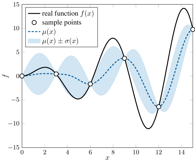
Figure 1: Gaussian process approximation of the function $f(x)=x\sin(x)$.

II-B Acquisition Function

The second major component of Bayesian optimization is the acquisition functions. After training the Gaussian process model, the following thing is to decide where to sample next in order to locate the global optimum of the original function as quickly as possible. This is done by maximizing a well-designed acquisition function in Bayesian optimization. To take a balance between global search and local search, the acquisition function should on one hand select points around current best observation and on the other hand select points around under-sample areas. Popular acquisition functions for Gaussian process models are the expected improvement [1], the probability of improvement [8], the lower confidence bound [9], the knowledge gradient [28, 29], and the entropy search [30, 31]. Among them, the expected improvement (EI) criterion is arguably the most widely used because of its mathematical tractability and good performance [26, 32]. Therefore, we focus on the EI acquisition function in this work.

Assume current minimum objective value among $n$ evaluated samples is $\min_{i=1}^{n}f(\bm{x}^{(i)})=f_{\min}$ and the corresponding best solution is $\arg\min_{i=1}^{n}f(\bm{x}^{(i)})=\bm{x}_{\min}$. According to the Gaussian process model, the objective value of an unknown point $\bm{x}$ can be interpreted as a random value following the normal distribution [2]

$$F(\bm{x})\sim N\left(\mu(\bm{x}),\sigma^{2}(\bm{x})\right)$$ (6)

where $\mu(\bm{x})$ and $\sigma^{2}(\bm{x})$ is the Gaussian process mean and variance in (4) and (5) respectively.

The EI function is the expectation of the improvement by comparing the random value $F(\bm{x})$ with $f_{\min}$ [2]

$$\text{EI}(\bm{x})=\mathbb{E}[\max(f_{\min}-F(\bm{x}),0)]$$ (7)

where $f_{\min}$ is current minimum objective value among all evaluated samples. Integrating this equation with the normal distribution in (6), we can get the closed-form expression [2]

$$\begin{split}\text{EI}(\bm{x})&=\left(f_{\min}-\mu(\bm{x})\right)\Phi\left(\frac{f_{\min}-\mu(\bm{x})}{\sigma(\bm{x})}\right)\\ &+\sigma(\bm{x})\phi\left(\frac{f_{\min}-\mu(\bm{x})}{\sigma(\bm{x})}\right)\end{split}$$ (8)

where $\Phi$ and $\phi$ are the standard normal cumulative and density functions respectively. As can be seen from the formula, the EI function is a nonlinear combination of the Gaussian process mean and variance.

The EI function of the one-dimensional example is shown in Fig. 2, where the solid line is the EI acquisition function and the open circles are the sample points. We can see that the EI function is zero at sampled points because sampling at these already evaluated points brings no improvement. We can also see that the EI function is high at places where the Gaussian process mean is low and the variance is high.

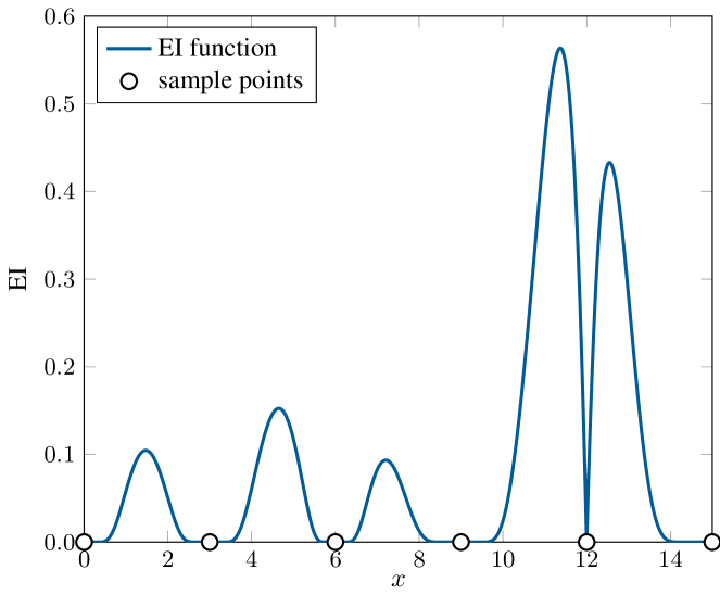
Figure 2: Expected improvement function of the function $f(x)=x\sin(x)$.

II-C Bayesian Optimization

Typically, Bayesian optimization works in a sequential way. Algorithm 1 shows the computational framework of Bayesian optimization. At the beginning of Bayesian optimization, a set of $n_{\text{init}}$ samples is drawn using some design of experiment method and evaluated with the expensive objective function. Then, Bayesian optimization works sequentially. In each iteration, the Gaussian process model is first trained using all the evaluated samples. Then, a new point is located by the acquisition function and evaluated with the expensive objective function. After that, Bayesian optimization goes to next iteration to query and evaluate another point. The sequential process stops when the maximum number of function evaluations $n_{\max}$ is reached. At the end, the algorithm outputs the best found solution $(\bm{x}_{\min},f_{\min})$.

Algorithm 1 Computational Framework of Bayesian optimization

0:  $n_{\text{init}}=$ number of initial samples; $n_{\max}=$ maximum number of objective evaluations.

0:  best found solution $(\bm{x}_{\min},f_{\min})$.

1:  Initial Design: generate $n_{\text{init}}$ samples $\bm{X}=[\bm{x}^{(1)},\bm{x}^{(2)},\cdots,\bm{x}^{(n_{\text{init}})}]$, evaluate them with the objective function $f(\bm{X})$, set current data set as $\mathcal{D}=(\bm{X},f(\bm{X}))$, set the best solution as $(\bm{x}_{\min},f_{\min})$ and set current number of evaluations $n=n_{\text{init}}$.

2:  while $n<n_{\max}$ do

3:     Model Training: train a GP model using the current data set $\mathcal{D}$.

4:     Acquisition Optimization: optimize the acquisition function to get next query point

$$\bm{x}^{(n+1)}={\underset{\bm{x}\in\mathcal{X}}{\arg\max}}~{}\text{EI}(\bm{x}).$$

5:     Expensive Evaluation: evaluate the query point to get $f(\bm{x}^{(n+1)})$.

6:     Best solution Update: update data set $\mathcal{D}=\{\mathcal{D},(\bm{x}^{(n+1)},f(\bm{x}^{(n+1)}))\}$, update current best solution as $(\bm{x}_{\min},f_{\min})$, and update current number of evaluations $n=n+1$.

7:  end while

III Proposed Approach

The standard Bayesian optimization selects one query point for expensive evaluation at each iteration. It can not utilize parallel computing techniques when multiple workers are available for doing the expensive evaluations. Current batch Bayesian optimization approaches are designed for small batch size. Their performances degenerate significantly when the batch size becomes large. In this work, we propose a novel batch Bayesian optimization that works well with large batch size. Different from ideas utilized by current batch approaches, our approach tries to select multiple query samples in multiple different subspaces. The new idea is easy to understand and the proposed algorithm is simple to implement.

III-A Expected Subspace Improvement

We propose a novel criterion named expected subspace improvement (ESSI) to select query points in subspaces. The proposed ESSI measures the improvement of a point in a specific subspace. Consider the original $d$-D design space

$$\mathcal{X}=\{[x_{1},x_{2},\cdots,x_{d}]\}\subseteq\mathbb{R}^{d},$$

an $s$-D ($1\leq s\leq d$) subspace can be expressed as

$$\mathcal{Y}=\{[y_{1},y_{2},\cdots,y_{s}]\}\subseteq\mathbb{R}^{s}$$

where $y_{i}\in\{x_{1},x_{2},\cdots,x_{d}\}$ for $i=1,2,\cdots,s$ and $y_{1}\neq y_{2}\neq\cdots,\neq y_{s}$. Assume the current best solution is $\bm{x}_{\min}=[x_{\min,1},x_{\min,2},\cdots,x_{\min,d}]$. The standard EI function measures the potential improvement a point can get beyond the current best solution $\bm{x}_{\min}$. From another point of view, the EI function can be seen as the measurement of the potential improvement as we move the current best solution $\bm{x}_{\min}$ in the original design space. Following this, we define the expected subspace improvement (ESSI) as the amount of expected improvement as we move the current best solution $\bm{x}_{\min}$ in a subspace

$$\begin{split}\text{ESSI}(\bm{y})&=\left(f_{\min}-\mu(\bm{z})\right)\Phi\left(\frac{f_{\min}-\mu(\bm{z})}{\sigma(\bm{z})}\right)\\ &+\sigma(\bm{z})\phi\left(\frac{f_{\min}-\mu(\bm{z})}{\sigma(\bm{z})}\right)\end{split}$$ (9)

where

$$\bm{z}=[x_{\min,1},\cdots,y_{1},\cdots,x_{\min,i}\cdots,y_{s},\cdots,x_{\min,d}]$$

is the $d$-D input of the Gaussian process model. In $\bm{z}$, the $y_{1},y_{2},\cdots,y_{d}$ are the coordinates of the subspace to be optimized and the remaining coordinates are fixed at the values of current best solution $\bm{x}_{\min}=[x_{\min,1},x_{\min,2},\cdots,x_{\min,d}]$.

We demonstrate the ESSI functions of the 3-D Rosenbrock problem in Fig. 3. We draw thirty random points in $[-2.048,2.048]^{3}$ and train a Gaussian process model using the sample points. We use the constant mean function and the squared exponential kernel function in the Gaussian process model, and search the best hyperparameter in the kernel function within $[0.01,100]$. The figure in the middle shows the scatter plots of the thirty samples in the original 3-D space. The red filled point is the current best solution among the thirty samples. On the left, we show the ESSI functions as we move the current best solution along coordinates $\bm{y}=x_{1}$, $\bm{y}=x_{2}$ and $\bm{y}=x_{3}$, respectively. On the right, we show the ESSI functions as we move the current best solution in subspaces $\bm{y}=[x_{1},x_{2}]$, $\bm{y}=[x_{1},x_{3}]$ and $\bm{y}=[x_{2},x_{3}]$, respectively. In other words, the left figures can be seen as the EI function in three 1-D subspaces while the right figures can be seen as the EI function in three 2-D subspaces.

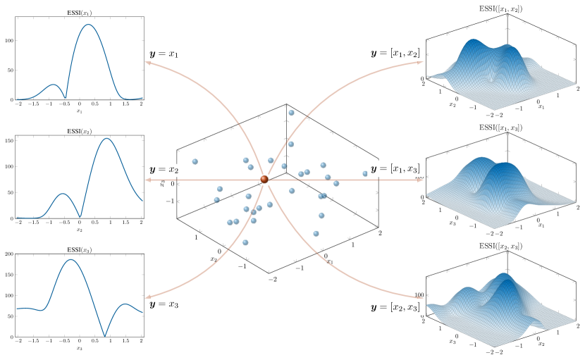
Figure 3: Six ESSI functions of a 3-D problem.

The dimension of the subspaces $s$ can vary from $1$ to $d$. When $s=d$, the proposed ESSI function is equal to the standard EI function [2]. And when $s=1$, the ESSI function degenerates to the expected coordinate improvement (ECI) function [33]. From this point of view, the proposed ESSI function can be seen as the more generalized measurement, and both the EI and ECI can be treated as especial cases of the ESSI function.

III-B Computational Framework

Algorithm 2 Computational Framework of the Proposed Batch Bayesian optimization

0:  $n_{\text{init}}=$ number of initial samples; $n_{\max}=$ maximum number of objective evaluations; $q=$ batch size.

0:  best found solution $(\bm{x}_{\min},f_{\min})$.

1:  Initial Design: generate $n_{\text{init}}$ samples $\bm{X}=[\bm{x}^{(1)},\bm{x}^{(2)},\cdots,\bm{x}^{(n_{\text{init}})}]$, evaluate them with the objective function $f(\bm{X})$, set current data set as $\mathcal{D}=(\bm{X},f(\bm{X}))$, set the best solution as $(\bm{x}_{\min},f_{\min})$ and set current number of evaluations $n=n_{\text{init}}$.

2:  while $n<n_{\max}$ do

3:     Model Training: train a GP model using the current data set $\mathcal{D}$.

4:     Subspace Selection: select $q$ subspaces randomly from all available subspaces

5:     for $i=1$ to $q$ do

6:        randomly draw an integer $s$ from 1 to $d$.

7:        randomly select $s$ variables from the original $d$ variables to get the subspace $\bm{y}^{(i)}$.

8:     end for

9:     Acquisition Optimization: optimize the $q$ ESSI functions to get $q$ query points

10:     for $i=1$ to $q$ do

11:        

$$\bm{y}_{\min}^{(i)}={\underset{\bm{y}^{(i)}\in\mathcal{Y}^{(i)}}{\arg\max}}~{}\text{ESSI}(\bm{y}^{(i)})$$

12:        replace coordinates in $\bm{x}_{\min}$ by $\bm{y}_{\min}^{(i)}$ to get $\bm{x}^{(n+i)}$.

13:     end for

14:     Expensive Evaluation: evaluate the $q$ query points in parallel to get $f(\bm{x}^{(n+1)}),\cdots,f(\bm{x}^{(n+q)})$.

15:     Best Solution Update: update data set $\mathcal{D}=\{\mathcal{D},(\bm{x}^{(n+1)},f(\bm{x}^{(n+1)})),\cdots,(\bm{x}^{(n+q)},f(\bm{x}^{(n+q)}))\}$, update current best solution as $(\bm{x}_{\min},f_{\min})$, and update current number of evaluations $n=n+q$.

16:  end while

Based on the proposed ESSI criterion, we propose a novel batch Bayesian optimization algorithm. The idea of the proposed approach is very simple. In each iteration, we locate a batch of $q$ points in $q$ different subspaces using the ESSI criterion, and then evaluate these $q$ query points in parallel. The computational framework of the proposed approach is given in Algorithm 2. The steps of the proposed algorithm are described as following.

1. Initial Design: The proposed batch Bayesian optimization algorithm also starts with an initial design. After getting the initial samples using some design of experiment method, we evaluate these samples with the real objective function. The current best solution $(\bm{x}_{\min},f_{\min})$ can be identified from the initial samples.

2. Model Training: Then the batch Bayesian optimization algorithm goes into the iteration process. At the beginning of each iteration, we first train a Gaussian process model using all evaluated samples. This step is the same as the standard Bayesian optimization algorithm.

3. Subspace Selection: Before locating a batch of query points in different subspaces, we should first determine the subspaces that we will select query points from. In this work, we use random selection approach to select a batch of subspaces.

4. Acquisition Optimization: After selecting a batch of subspaces, we can then locate one query point within one subspace by optimizing the corresponding ESSI function. Since these ESSI functions are independent from each other, we can solve these ESSI optimization problems in parallel.

5. Expensive Evaluation: Optimizing the $q$ ESSI functions delivers $q$ different query points. In this step, we can then evaluate these $q$ query points with the expensive objective function in parallel. Since the most time-consuming step of Bayesian optimization is often the expensive evaluation step, distributing the query points in different machines and evaluating them in parallel can save us a lot of wall-clock time.

6. Best Solution Update: At the end of the iteration, we need to update the data set by including the newly evaluated samples. We also need to update the best solution since it will be used in the next round of iterations. After the update, the algorithm goes back to the model training for a new iteration. The iteration process stops when the maximal number of function evaluations is reached.

The major difference between our proposed batch Bayesian optimization algorithm and the standard Bayesian optimization algorithm is that in each iteration the standard approach selects one query point in the original design space while our batch approach selects multiple query points in different subspaces. Therefore, the standard approach can only evaluate the query points one by one while the proposed batch approach can evaluate them in parallel. The subspace selection and acquisition optimization are the two key steps for our proposed batch Bayesian optimization algorithm, therefore are further discussed in the following in detail.

III-C Subspace Selection

In subspace selection, we employ the most straightforward method, that is selecting the subspaces randomly. This random selection strategy avoids setting the hyper-parameter $s$ (the dimension of the subspace) and turns out to be very efficient. The dimension of the subspace $s$ can vary from 1 to $d$. When $s=1$, the available subspaces are $\{[x_{1}],[x_{2}],\cdots,[x_{d}]\}$. Similarly, as $s=2$, the available subspaces are $\{[x_{1},x_{2}],[x_{1},x_{3}],\cdots,[x_{d-1},x_{d}]\}$. This goes on until $s$ reaches to $d$, in which case there is only one available subspace $\{[x_{1},x_{2},\cdots,x_{d}]\}$. The total number of subspaces of a $d$-D space can be calculated as

$$N=C_{1}^{d}+C_{2}^{d}+\cdots+C_{d}^{d}=2^{d}-1$$

where $C_{i}^{d}$ donates the number of combinations of selecting $i$ different variables from $d$ total variables. The number $N$ is very large when the dimension of the original space is not that small. For example, the total number of subspaces of a $10$-D space is $N=2^{10}-1=1023$, which is much larger than the batch size we commonly use. In the cases where $N$ is smaller than the batch size $q$, we can employ existing strategy such as Kriging Believer or Constant Liar [11] to select multiple points within one subspace.

Instead of directly drawing $q$ subspaces from all $N$ subspaces, we select the $q$ subspaces by first drawing a random integer and then drawing a random combination, as shown in the Step 6 and Step 7 in Algorithm 2. The reason is that the direct selection strategy is very computationally expensive to list all $N$ subspaces when $d$ is large. Our strategy is very fast but might select identical subspaces during the $q$ selections. One can eliminate this by checking whether the candidate subspace has been selected after each selection. If the candidate subspace has been selected, then we can reject the selection and start a new drawing. When the dimension of the problem $d$ is larger than 20, the probability of selecting identical subspace can be neglected.

III-D Acquisition Optimization

In the acquisition optimization process, we optimize the variables of $i$th subspace while holding the other variables fixed at the current best solution $\bm{x}_{\min}$. After the optimization, we replace the variables in $\bm{x}_{\min}$ by the optimized ones to get the $i$th query point

$$\begin{split}&\bm{x}^{(n+i)}=\\ &[x_{\min,1},\cdots,y^{(i)}_{\min,1},\cdots,x_{\min,i}\cdots,y^{(i)}_{\min,s},\cdots,x_{\min,d}].\end{split}$$

We demonstrate the acquisition optimization process also on a 3-D example in Fig. 4. Assume that the current best solution is $\bm{x}_{\min}=[x_{\min,1},x_{\min,2},x_{\min,3}]$, and the six subspaces we select are $\bm{y}^{(1)}=x_{1}$, $\bm{y}^{(2)}=x_{2}$, $\bm{y}^{(3)}=x_{3}$, $\bm{y}^{(4)}=[x_{1},x_{2}]$, $\bm{y}^{(5)}=[x_{1},x_{3}]$ and $\bm{y}^{(6)}=[x_{2},x_{3}]$.

For the first acquisition optimization problem, the optimizing variable is $x_{1}$. After the optimization process, we can get the result

$$y^{(1)}_{\min,1}={\underset{x_{1}\in[a_{1},b_{1}]}{\arg\max}}~{}\text{ESSI}(x_{1}).$$

Then we replace the $x_{1}$ coordinate of the current best solution by this optimized variable and get our first query point

$$\bm{x}^{(n+1)}=[y^{(1)}_{\min,1},x_{\min,2},x_{\min,3}].$$

Following the same procedure, we can get our second and third query points by optimizing $x_{2}$ and $x_{3}$ variables, respectively.

For the fourth acquisition optimization problem, the subspaces we select are $\bm{y}^{(4)}=[x_{1},x_{2}]$. After solving this two-variable optimization problem, we can get

$$[y^{(4)}_{\min,1},y^{(4)}_{\min,2}]={\underset{x_{1}\in[a_{1},b_{1}],x_{2}\in[a_{2},b_{2}]}{\arg\max}}~{}\text{ESSI}([x_{1},x_{2}]).$$

Then, we replace the $x_{1}$ and $x_{2}$ coordinates of the current best solution by the two optimized variables to get our fourth query point

$$\bm{x}^{(n+4)}=[y^{(4)}_{\min,1},y^{(4)}_{\min,2},x_{\min,3}].$$

Similarly, we can get our fifth and sixth query points by optimizing $[x_{1},x_{3}]$ and $[x_{2},x_{3}]$, respectively.

Figure 4: Acquisition optimization results on a 3-D problem.

From the above discussion, we can also find that these $q$ acquisition optimization problems are mutually independent. Therefore, we can solve them in parallel. This might be beneficial to the computational time when the batch size is large compared with batch approaches that optimize $q$ acquisition functions sequentially.

Since the dimension of the subspace $s$ is randomly drawn from 1 to $d$

$$S\sim U(1,d)$$

the expectation of $S$ is then $\mathbb{E}(S)=\frac{1+d}{2}$. Therefore, on average the dimension of our ESSI functions are near half of the dimension of the original problem. This might make our ESSI functions easier to solve compared with the original EI function.

IV Numerical Experiments

In this section, we conduct two sets of experiments to verify the effectiveness of our proposed ESSI approach. In the first set of experiments, we compare the proposed batch approach with the sequential approach to see the speedup of the proposed approach. In the second set of experiments, we compare the proposed ESSI approach with eight existing batch algorithms to see how well the proposed approach performs when compared with the state-of-the-art.

IV-A Experiment Settings

We use the CEC 2017 test suite [34] as the benchmark problems. All the 29 problems in the test suite are rotated and shifted. In the test suite, the $f_{1}$ and $f_{3}$ are unimodal functions, $f_{4}$ to $f_{10}$ are multimodal functions, $f_{11}$ to $f_{20}$ are hybrid functions, and $f_{21}$ to $f_{30}$ are composition functions [34]. The dimensions of all the test problems are set to $d=100$.

The Latin hypercube sampling is used to generate the initial samples for the compared algorithms. The number of initial samples is set to $n_{\text{init}}=200$. For the Gaussian process model, we use the constant mean function and the square exponential kernel function. We maximize the log-likelihood of the observed samples to estimate the parameters of the Gaussian process model.

For all experiments, the number of acquisition samples is set $1024$, therefore the maximum number of objective evaluations is $n_{\max}=200+1024=1224$. Since the acquisition functions are often highly multimodal, we employ a real-coded genetic algorithm to maximize the EI and ESSI functions. The population size of the genetic algorithm is set to twice as the dimension, and the maximal number of generation is set to $100$. We use simulated binary crossover and polynomial mutation in the genetic algorithm. The crossover rate is set to $0.9$ and the mutation rate is set to $1/d$. Both the distribution indices for the crossover and mutation are set to $20$.

All experiments are run $30$ times to deliver reliable results. The initial sample sets are different for $30$ runs, and are the same for different compared algorithms.

All experiments are run on a Window 10 machine which has two Intel Xeon Gold 6338 CPUs (a total of 64 physical cores) and 128 GB RAM. All experiments are conducted using MATLAB R2022b.

IV-B Comparison with Sequential BO Algorithm

We first compare the proposed ESSI with the standard EI to study the speedup of the proposed approach. We set $q$ to $2$, $4$, $8$, $16$, $32$ and $64$ respectively to test the performance of the proposed approach under different batch sizes. Since the number of acquisition samples is fixed as $1024$, the corresponding maximal iterations for the batch algorithm are then $512$, $256$, $128$, $64$, $32$ and $16$, respectively.

The final optimization results of the standard EI approach and the ESSI approach are presented in Table I, where the average values of 30 runs are given. We conduct the Wilcoxon signed rank test to find out whether the results obtained by the proposed ESSI have significantly difference from the results obtained by the standard EI. The significance level of the tests is set to $\alpha=0.05$. We use $+$, $-$ and $\approx$ to represent that our ESSI approach finds significantly better, significantly worse and similar results compared with the sequential EI approach, respectively.

From Table I we can see that the proposed batch ESSI approach finds significantly better results than the sequential EI approach on most of the test problems at the end of 1024 additional function evaluations. By locating new samples in lower-dimensional subspaces, the proposed ESSI approach reduces the difficulty of optimizing the acquisition function compared with the standard EI approach which finds new samples in the original space. The significant tests show that our proposed ESSI approach is able to achieve better results than the standard EI approach on twenty-six, twenty-six, twenty-four, twenty-five, twenty-five and twenty-five test problems as the batch size of $2$, $4$, $8$, $16$, $32$ and $64$ is utilized, respectively. The experiment results can empirically prove the effectiveness of the proposed ESSI approach.

TABLE I: Average results obtained by the compared EI and ESSI approaches on the test problems

$f$	EI	ESSI
		$q=2$	$q=4$	$q=8$	$q=16$	$q=32$	$q=64$
$f_{1}$	1.10E+10	3.71E+08 $+$	3.46E+08 $+$	3.58E+08 $+$	4.08E+08 $+$	6.26E+08 $+$	1.07E+09 $+$
$f_{3}$	1.13E+06	1.28E+06 $\approx$	1.29E+06 $\approx$	1.02E+06 $\approx$	1.21E+06 $\approx$	3.14E+06 $-$	1.29E+06 $\approx$
$f_{4}$	1.35E+04	4.05E+03 $+$	4.05E+03 $+$	4.08E+03 $+$	4.44E+03 $+$	4.82E+03 $+$	5.46E+03 $+$
$f_{5}$	1.60E+03	1.23E+03 $+$	1.26E+03 $+$	1.32E+03 $+$	1.41E+03 $+$	1.48E+03 $+$	1.55E+03 $+$
$f_{6}$	6.63E+02	6.56E+02 $+$	6.55E+02 $+$	6.54E+02 $+$	6.50E+02 $+$	6.48E+02 $+$	6.46E+02 $+$
$f_{7}$	2.23E+03	2.47E+03 $-$	2.44E+03 $-$	2.39E+03 $-$	2.32E+03 $-$	2.27E+03 $\approx$	2.29E+03 $-$
$f_{8}$	1.90E+03	1.59E+03 $+$	1.65E+03 $+$	1.71E+03 $+$	1.77E+03 $+$	1.79E+03 $+$	1.84E+03 $+$
$f_{9}$	4.07E+04	4.44E+04 $\approx$	4.14E+04 $\approx$	4.01E+04 $\approx$	4.00E+04 $\approx$	3.56E+04 $+$	3.66E+04 $+$
$f_{10}$	3.44E+04	2.15E+04 $+$	2.19E+04 $+$	2.16E+04 $+$	2.16E+04 $+$	2.19E+04 $+$	2.31E+04 $+$
$f_{11}$	4.64E+05	3.82E+05 $+$	3.73E+05 $+$	3.82E+05 $+$	3.65E+05 $+$	3.51E+05 $+$	3.59E+05 $+$
$f_{12}$	1.41E+10	1.92E+09 $+$	1.84E+09 $+$	1.85E+09 $+$	2.47E+09 $+$	2.20E+09 $+$	3.26E+09 $+$
$f_{13}$	3.81E+09	6.64E+08 $+$	6.66E+08 $+$	7.63E+08 $+$	9.54E+08 $+$	1.30E+09 $+$	1.08E+09 $+$
$f_{14}$	7.87E+07	6.38E+07 $+$	6.48E+07 $+$	7.01E+07 $\approx$	6.00E+07 $+$	7.48E+07 $\approx$	7.67E+07 $\approx$
$f_{15}$	3.61E+09	9.88E+08 $+$	8.01E+08 $+$	7.64E+08 $+$	1.02E+09 $+$	7.13E+08 $+$	7.46E+08 $+$
$f_{16}$	1.24E+04	1.14E+04 $+$	1.12E+04 $+$	1.15E+04 $+$	1.14E+04 $+$	1.15E+04 $+$	1.16E+04 $+$
$f_{17}$	5.80E+05	1.18E+05 $+$	1.57E+05 $+$	1.16E+05 $+$	1.40E+05 $+$	1.37E+05 $+$	2.02E+05 $+$
$f_{18}$	1.15E+08	7.39E+07 $+$	6.60E+07 $+$	7.63E+07 $+$	9.71E+07 $\approx$	9.18E+07 $+$	8.64E+07 $+$
$f_{19}$	2.95E+09	1.42E+09 $+$	1.22E+09 $+$	1.24E+09 $+$	1.14E+09 $+$	8.77E+08 $+$	8.49E+08 $+$
$f_{20}$	8.78E+03	6.86E+03 $+$	6.79E+03 $+$	6.62E+03 $+$	6.76E+03 $+$	6.79E+03 $+$	6.94E+03 $+$
$f_{21}$	3.56E+03	3.50E+03 $+$	3.50E+03 $+$	3.53E+03 $\approx$	3.52E+03 $+$	3.54E+03 $\approx$	3.57E+03 $\approx$
$f_{22}$	3.70E+04	2.41E+04 $+$	2.38E+04 $+$	2.41E+04 $+$	2.42E+04 $+$	2.40E+04 $+$	2.55E+04 $+$
$f_{23}$	4.14E+03	4.02E+03 $+$	3.98E+03 $+$	4.00E+03 $+$	4.00E+03 $+$	4.04E+03 $+$	4.07E+03 $+$
$f_{24}$	4.58E+03	4.52E+03 $+$	4.50E+03 $+$	4.49E+03 $+$	4.49E+03 $+$	4.49E+03 $+$	4.52E+03 $+$
$f_{25}$	1.17E+04	6.08E+03 $+$	6.17E+03 $+$	6.17E+03 $+$	6.35E+03 $+$	6.65E+03 $+$	7.16E+03 $+$
$f_{26}$	2.18E+04	1.98E+04 $+$	1.98E+04 $+$	1.97E+04 $+$	1.95E+04 $+$	1.96E+04 $+$	2.01E+04 $+$
$f_{27}$	4.52E+03	3.92E+03 $+$	3.89E+03 $+$	3.92E+03 $+$	3.96E+03 $+$	4.05E+03 $+$	4.15E+03 $+$
$f_{28}$	1.46E+04	6.54E+03 $+$	6.63E+03 $+$	6.89E+03 $+$	7.28E+03 $+$	8.23E+03 $+$	9.80E+03 $+$
$f_{29}$	3.97E+05	8.25E+04 $+$	1.29E+05 $+$	1.10E+05 $+$	1.07E+05 $+$	1.16E+05 $+$	1.67E+05 $+$
$f_{30}$	8.04E+09	3.54E+09 $+$	3.31E+09 $+$	3.00E+09 $+$	2.70E+09 $+$	2.12E+09 $+$	2.16E+09 $+$
$+$/$\approx$/$-$	N.A.	26/2/1	26/2/1	24/4/1	25/3/1	25/3/1	25/3/1

The convergence curves of the standard EI and the proposed ESSI approaches on the test problems are shown in Fig. 5, where the horizontal axis is the number of iterations and the vertical axis is the found minimal objective value. In these figures, we show the median, the first quartile, and the third quartile of the $30$ runs.

From the curves we can see that the proposed ESSI approach converges much faster than the standard EI approach on the tested problems. The batch approach evaluates $q$ points in each iteration, therefore it only needs $1024/q$ iterations to finish all the function evaluations. By distributing the evaluations on multiple cores or machines, the batch approach is able to reduce the wall-clock $q$ times compared with the sequential approach. We can also see that the convergence speed of the proposed ESSI approach can be further improved as we increase the batch size from $2$ to $64$, which shows the good scalability of the proposed ESSI approach with respect to the batch size. At the end of $1024$ additional function evaluations, the proposed ESSI approach even finds better solutions than the standard EI approach on most of the test problems. This means the proposed ESSI approach is able to reduce the wall-clock time and improve the optimization results at the same time.

() $f_{1}$

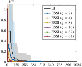
() $f_{3}$

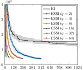
() $f_{4}$

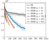
() $f_{5}$

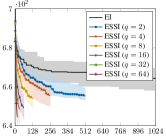
() $f_{6}$

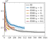
() $f_{7}$

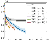
() $f_{8}$

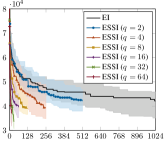
() $f_{9}$

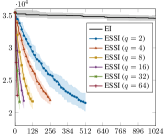
() $f_{10}$

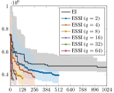
() $f_{11}$

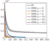
() $f_{12}$

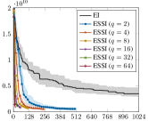
() $f_{13}$

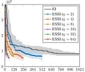
() $f_{14}$

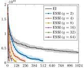
() $f_{15}$

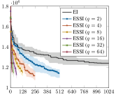
() $f_{16}$

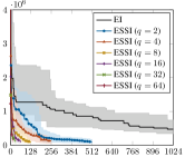
() $f_{17}$

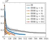
() $f_{18}$

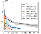
() $f_{19}$

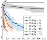
() $f_{20}$

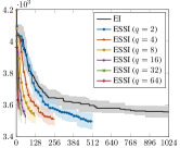
() $f_{21}$

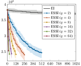
() $f_{22}$

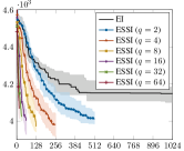
() $f_{23}$

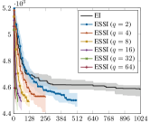
() $f_{24}$

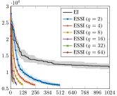
() $f_{25}$

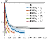
() $f_{26}$

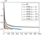
() $f_{27}$

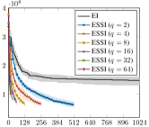
() $f_{28}$

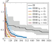
() $f_{29}$

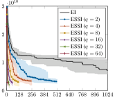
() $f_{30}$

Figure 5: Convergence plots of the standard EI and the proposed ESSI on the test problems.

Then, we compare the running time of the proposed ESSI approach and the standard EI approach. The running time of both the ESSI and the EI consists of the time of training the GP model, optimizing the acquisition functions and evaluating the new points. For the model training, the standard EI needs to train the GP model $1024$ times while the ESSI approach only needs to train the GP model $1024/q$ times as it evaluates $q$ query points at each iteration. For the acquisition optimization, the standard EI approach optimizes one EI function at a time while the ESSI approach optimizes $q$ ESSI functions within one iteration. For the function evaluation, the standard EI approach evaluates one new sample in each iteration while the ESSI approach evaluates $q$ new samples. Both the $q$ acquisition optimizations and function evaluations of the ESSI approach can be executed in parallel. In the experiments, we use MATLAB parfor to distribute the $q$ acquisition optimizations and function evaluations on $q$ CPU cores, and run them in parallel.

The running time comparison is presented in Fig. 6, where the vertical axis is the average running time of 30 runs and is shown in seconds. We can see that the proposed ESSI approach is able to reduce the running time significantly compared with the standard EI approach. As the batch size $q$ increases, the running time of ESSI decreases gradually. The speedup ratio of ESSI is around $1.86$, $3.04$, $5.04$, $8.69$, $14.32$ and $17.77$ for $q=2,4,8,16,32$ and $64$, respectively. This means the speedup of ESSI is under-linear. The reason that the ESSI approach is not able to achieve linear speedup is that the ESSI requires some computational time to select subspaces in each iteration. It should be noted that the time for training the GP model and optimizing the acquisition function can often be neglected when compared with evaluating expensive simulations. The ESSI approach should be able to achieve near linear speedup by evaluating the expensive simulations in parallel.

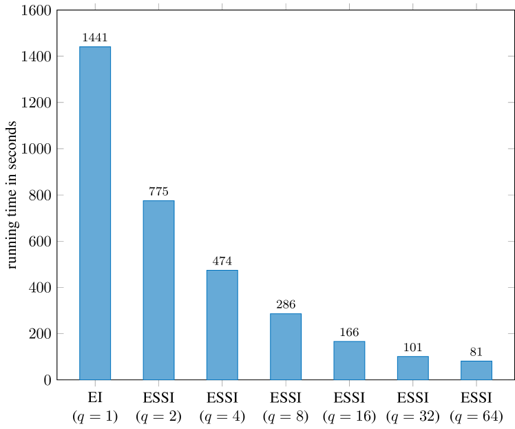
Figure 6: Running time of the standard EI and the proposed ESSI on the test problems.

IV-C Comparison with Batch Approaches

In the second set of experiments, we compare the proposed ESSI approach with eight batch approaches, which include four batch Bayesian optimization algorithms and four batch surrogate-assisted evolutionary algorithms (SAEAs). The four batch BOs are the Kriging believer (KB) [11], constant liar (CL) [11], expected improvement and mutual information (EIMI) [17], and fast multipoint expected improvement (F$q$-EI) [15]. The four compared batch SAEAs are Gaussian process-assisted differential evolution (GPDE), Gaussian process surrogate model assisted evolutionary algorithm for medium-scale computationally expensive optimization problems (GPEME) [35], incremental Kriging-assisted evolutionary algorithm (IKAEA) [36], and Kriging-assisted evolutionary algorithm based on anisotropic expected improvement (KAEA-AEI) [37]. All the compared algorithms use Gaussian process models as the surrogate models. Among the batch BOs, the KB, CL and EIMI approaches are sequential-batch approaches. This means they optimize the acquisition functions sequentially to get $q$ points and evaluate them in parallel. The F$q$-EI approach gets all the $q$ new points at once by optimizing a $q\times d$ acquisition function. The GPDE approach uses the GP model as the surrogate and the differential evolution algorithm as the base EA. It uses the EI function to measure the quality of the individuals and select the $q$ best individuals to do expensive evaluations. The GPEME uses the lower confidence bound (LCB) function to select the individuals for expensive evaluations. The IKAEA uses incremental learning approach to train the model and also uses the EI function to select individuals to do expensive evaluations. Finally, the KAEA-AEI uses the anisotropic expected improvement function to select individuals for expensive evaluations. The population size of all the four SAEAs is set $100$. We set the batch size to $q=4,16$ and $64$ to test the algorithms’ performances under small, medium and large batch sizes, respectively.

TABLE II: Average results obtained by the compared batch approaches with $q=4$ on the test problems

$f$	KB	CL	EIMI	F$q$-EI	GPDE	GPEME	IKAEA	KAEA-AEI	ESSI
$f_{1}$	1.13E+10 $+$	1.22E+10 $+$	1.10E+10 $+$	1.24E+10 $+$	2.04E+11 $+$	1.19E+11 $+$	1.20E+11 $+$	1.91E+11 $+$	3.46E+08
$f_{3}$	1.36E+06 $\approx$	9.29E+05 $\approx$	1.02E+06 $\approx$	1.08E+06 $\approx$	1.64E+06 $\approx$	4.25E+06 $\approx$	2.14E+06 $\approx$	2.86E+06 $\approx$	1.29E+06
$f_{4}$	1.32E+04 $+$	1.29E+04 $+$	1.34E+04 $+$	1.52E+04 $+$	4.79E+04 $+$	2.89E+04 $+$	2.95E+04 $+$	4.78E+04 $+$	4.05E+03
$f_{5}$	1.73E+03 $+$	1.62E+03 $+$	1.71E+03 $+$	1.65E+03 $+$	2.03E+03 $+$	1.86E+03 $+$	1.83E+03 $+$	1.98E+03 $+$	1.26E+03
$f_{6}$	6.64E+02 $+$	6.64E+02 $+$	6.65E+02 $+$	6.55E+02 $\approx$	7.02E+02 $+$	6.86E+02 $+$	6.86E+02 $+$	7.00E+02 $+$	6.55E+02
$f_{7}$	2.28E+03 $-$	2.30E+03 $-$	2.30E+03 $-$	2.13E+03 $-$	4.59E+03 $+$	3.37E+03 $+$	3.33E+03 $+$	4.39E+03 $+$	2.44E+03
$f_{8}$	2.00E+03 $+$	1.91E+03 $+$	2.01E+03 $+$	1.94E+03 $+$	2.38E+03 $+$	2.20E+03 $+$	2.19E+03 $+$	2.34E+03 $+$	1.65E+03
$f_{9}$	4.82E+04 $+$	4.18E+04 $\approx$	4.66E+04 $+$	3.57E+04 $-$	8.83E+04 $+$	7.00E+04 $+$	6.40E+04 $+$	8.48E+04 $+$	4.14E+04
$f_{10}$	3.43E+04 $+$	3.45E+04 $+$	3.45E+04 $+$	3.44E+04 $+$	3.43E+04 $+$	3.42E+04 $+$	3.42E+04 $+$	3.44E+04 $+$	2.19E+04
$f_{11}$	4.38E+05 $+$	4.90E+05 $+$	3.94E+05 $\approx$	4.78E+05 $+$	4.18E+05 $+$	3.86E+05 $\approx$	4.12E+05 $\approx$	4.23E+05 $+$	3.73E+05
$f_{12}$	1.36E+10 $+$	1.40E+10 $+$	1.41E+10 $+$	1.93E+10 $+$	8.53E+10 $+$	4.82E+10 $+$	4.65E+10 $+$	8.53E+10 $+$	1.84E+09
$f_{13}$	4.05E+09 $+$	3.69E+09 $+$	3.57E+09 $+$	5.80E+09 $+$	1.61E+10 $+$	7.31E+09 $+$	6.67E+09 $+$	1.42E+10 $+$	6.66E+08
$f_{14}$	8.18E+07 $+$	9.10E+07 $+$	7.90E+07 $+$	1.04E+08 $+$	1.87E+08 $+$	1.46E+08 $+$	1.51E+08 $+$	1.85E+08 $+$	6.48E+07
$f_{15}$	3.52E+09 $+$	3.20E+09 $+$	3.43E+09 $+$	4.67E+09 $+$	5.72E+09 $+$	2.90E+09 $+$	2.37E+09 $+$	5.78E+09 $+$	8.01E+08
$f_{16}$	1.23E+04 $+$	1.25E+04 $+$	1.24E+04 $+$	1.29E+04 $+$	1.55E+04 $+$	1.39E+04 $+$	1.36E+04 $+$	1.51E+04 $+$	1.12E+04
$f_{17}$	6.11E+05 $+$	6.37E+05 $+$	6.31E+05 $+$	7.92E+05 $+$	4.35E+05 $+$	2.94E+05 $+$	1.78E+05 $\approx$	4.51E+05 $+$	1.57E+05
$f_{18}$	1.18E+08 $+$	9.89E+07 $+$	1.11E+08 $+$	1.32E+08 $+$	2.88E+08 $+$	2.57E+08 $+$	2.46E+08 $+$	2.91E+08 $+$	6.60E+07
$f_{19}$	3.00E+09 $+$	2.89E+09 $+$	2.94E+09 $+$	3.80E+09 $+$	7.08E+09 $+$	3.02E+09 $+$	2.74E+09 $+$	5.87E+09 $+$	1.22E+09
$f_{20}$	8.78E+03 $+$	8.77E+03 $+$	8.85E+03 $+$	8.77E+03 $+$	8.48E+03 $+$	8.73E+03 $+$	8.52E+03 $+$	8.74E+03 $+$	6.79E+03
$f_{21}$	3.59E+03 $+$	3.60E+03 $+$	3.60E+03 $+$	3.56E+03 $+$	4.13E+03 $+$	3.88E+03 $+$	3.94E+03 $+$	4.10E+03 $+$	3.50E+03
$f_{22}$	3.69E+04 $+$	3.71E+04 $+$	3.71E+04 $+$	3.68E+04 $+$	3.65E+04 $+$	3.68E+04 $+$	3.66E+04 $+$	3.68E+04 $+$	2.38E+04
$f_{23}$	4.19E+03 $+$	4.17E+03 $+$	4.21E+03 $+$	4.22E+03 $+$	5.61E+03 $+$	5.38E+03 $+$	5.39E+03 $+$	5.53E+03 $+$	3.98E+03
$f_{24}$	4.61E+03 $+$	4.60E+03 $+$	4.64E+03 $+$	4.72E+03 $+$	8.23E+03 $+$	7.41E+03 $+$	7.31E+03 $+$	7.97E+03 $+$	4.50E+03
$f_{25}$	1.15E+04 $+$	1.16E+04 $+$	1.16E+04 $+$	1.27E+04 $+$	2.63E+04 $+$	1.60E+04 $+$	1.57E+04 $+$	2.32E+04 $+$	6.17E+03
$f_{26}$	2.19E+04 $+$	2.17E+04 $+$	2.19E+04 $+$	2.28E+04 $+$	4.12E+04 $+$	3.45E+04 $+$	3.33E+04 $+$	4.06E+04 $+$	1.98E+04
$f_{27}$	4.56E+03 $+$	4.56E+03 $+$	4.53E+03 $+$	4.68E+03 $+$	9.29E+03 $+$	8.63E+03 $+$	8.57E+03 $+$	9.21E+03 $+$	3.89E+03
$f_{28}$	1.45E+04 $+$	1.46E+04 $+$	1.47E+04 $+$	1.60E+04 $+$	2.99E+04 $+$	2.26E+04 $+$	2.19E+04 $+$	2.93E+04 $+$	6.63E+03
$f_{29}$	3.21E+05 $+$	3.42E+05 $+$	4.01E+05 $+$	3.92E+05 $+$	2.63E+05 $+$	1.22E+05 $\approx$	1.34E+05 $\approx$	2.90E+05 $+$	1.29E+05
$f_{30}$	7.51E+09 $+$	7.28E+09 $+$	7.59E+09 $+$	9.04E+09 $+$	1.32E+10 $+$	6.90E+09 $+$	6.09E+09 $+$	1.24E+10 $+$	3.31E+09
$+$/$\approx$/$-$	27/1/1	26/2/1	26/2/1	25/2/2	28/1/0	26/3/0	25/4/0	28/1/0	N.A.

TABLE III: Average results obtained by the compared batch approaches with $q=16$ on the test problems

$f$	KB	CL	EIMI	F$q$-EI	GPDE	GPEME	IKAEA	KAEA-AEI	ESSI
$f_{1}$	1.12E+10 $+$	1.31E+10 $+$	1.21E+10 $+$	1.40E+10 $+$	3.33E+11 $+$	3.18E+11 $+$	3.14E+11 $+$	3.44E+11 $+$	4.08E+08
$f_{3}$	9.38E+05 $\approx$	9.53E+05 $\approx$	9.33E+05 $-$	2.11E+06 $\approx$	1.95E+06 $\approx$	2.57E+06 $\approx$	1.61E+06 $\approx$	1.38E+07 $+$	1.21E+06
$f_{4}$	1.32E+04 $+$	1.34E+04 $+$	1.30E+04 $+$	1.76E+04 $+$	1.07E+05 $+$	1.01E+05 $+$	9.67E+04 $+$	1.09E+05 $+$	4.44E+03
$f_{5}$	1.88E+03 $+$	1.59E+03 $+$	1.88E+03 $+$	1.69E+03 $+$	2.37E+03 $+$	2.34E+03 $+$	2.32E+03 $+$	2.37E+03 $+$	1.41E+03
$f_{6}$	6.64E+02 $+$	6.61E+02 $+$	6.63E+02 $+$	6.58E+02 $+$	7.24E+02 $+$	7.21E+02 $+$	7.22E+02 $+$	7.23E+02 $+$	6.50E+02
$f_{7}$	2.31E+03 $\approx$	2.30E+03 $\approx$	2.37E+03 $+$	2.21E+03 $-$	7.47E+03 $+$	6.98E+03 $+$	6.93E+03 $+$	7.14E+03 $+$	2.32E+03
$f_{8}$	2.25E+03 $+$	1.89E+03 $+$	2.21E+03 $+$	1.99E+03 $+$	2.77E+03 $+$	2.68E+03 $+$	2.68E+03 $+$	2.73E+03 $+$	1.77E+03
$f_{9}$	4.85E+04 $+$	4.23E+04 $\approx$	4.77E+04 $+$	4.51E+04 $+$	1.37E+05 $+$	1.31E+05 $+$	1.25E+05 $+$	1.37E+05 $+$	4.00E+04
$f_{10}$	3.43E+04 $+$	3.46E+04 $+$	3.45E+04 $+$	3.44E+04 $+$	3.41E+04 $+$	3.44E+04 $+$	3.42E+04 $+$	3.41E+04 $+$	2.16E+04
$f_{11}$	3.48E+05 $\approx$	4.59E+05 $+$	4.09E+05 $+$	4.93E+05 $+$	4.26E+05 $+$	4.20E+05 $+$	4.34E+05 $+$	3.98E+05 $\approx$	3.65E+05
$f_{12}$	1.37E+10 $+$	1.29E+10 $+$	1.44E+10 $+$	1.89E+10 $+$	1.73E+11 $+$	1.50E+11 $+$	1.45E+11 $+$	1.63E+11 $+$	2.47E+09
$f_{13}$	3.41E+09 $+$	3.37E+09 $+$	3.39E+09 $+$	6.11E+09 $+$	3.73E+10 $+$	3.40E+10 $+$	3.27E+10 $+$	3.47E+10 $+$	9.54E+08
$f_{14}$	6.91E+07 $\approx$	8.39E+07 $+$	7.25E+07 $\approx$	1.06E+08 $+$	2.50E+08 $+$	2.51E+08 $+$	2.13E+08 $+$	2.21E+08 $+$	6.00E+07
$f_{15}$	2.97E+09 $+$	3.19E+09 $+$	2.60E+09 $+$	4.96E+09 $+$	1.51E+10 $+$	1.48E+10 $+$	1.39E+10 $+$	1.44E+10 $+$	1.02E+09
$f_{16}$	1.24E+04 $+$	1.25E+04 $+$	1.26E+04 $+$	1.29E+04 $+$	2.02E+04 $+$	1.94E+04 $+$	1.88E+04 $+$	1.94E+04 $+$	1.14E+04
$f_{17}$	6.83E+05 $+$	5.55E+05 $+$	6.18E+05 $+$	9.79E+05 $+$	1.86E+06 $+$	1.41E+06 $+$	9.47E+05 $+$	1.58E+06 $+$	1.40E+05
$f_{18}$	9.85E+07 $\approx$	1.12E+08 $\approx$	7.63E+07 $\approx$	1.36E+08 $+$	4.50E+08 $+$	4.73E+08 $+$	3.94E+08 $+$	4.36E+08 $+$	9.71E+07
$f_{19}$	2.51E+09 $+$	2.78E+09 $+$	2.61E+09 $+$	4.06E+09 $+$	1.53E+10 $+$	1.41E+10 $+$	1.42E+10 $+$	1.59E+10 $+$	1.14E+09
$f_{20}$	8.73E+03 $+$	8.78E+03 $+$	8.74E+03 $+$	8.82E+03 $+$	8.61E+03 $+$	8.70E+03 $+$	8.60E+03 $+$	8.78E+03 $+$	6.76E+03
$f_{21}$	3.67E+03 $+$	3.60E+03 $+$	3.72E+03 $+$	3.59E+03 $+$	4.58E+03 $+$	4.49E+03 $+$	4.50E+03 $+$	4.52E+03 $+$	3.52E+03
$f_{22}$	3.68E+04 $+$	3.70E+04 $+$	3.69E+04 $+$	3.70E+04 $+$	3.68E+04 $+$	3.67E+04 $+$	3.68E+04 $+$	3.69E+04 $+$	2.42E+04
$f_{23}$	4.30E+03 $+$	4.21E+03 $+$	4.31E+03 $+$	4.25E+03 $+$	6.29E+03 $+$	6.18E+03 $+$	6.24E+03 $+$	6.30E+03 $+$	4.00E+03
$f_{24}$	4.75E+03 $+$	4.62E+03 $+$	4.74E+03 $+$	4.79E+03 $+$	9.89E+03 $+$	9.55E+03 $+$	9.71E+03 $+$	9.85E+03 $+$	4.49E+03
$f_{25}$	1.16E+04 $+$	1.21E+04 $+$	1.17E+04 $+$	1.33E+04 $+$	5.07E+04 $+$	4.71E+04 $+$	4.69E+04 $+$	4.95E+04 $+$	6.35E+03
$f_{26}$	2.23E+04 $+$	2.20E+04 $+$	2.27E+04 $+$	2.37E+04 $+$	5.30E+04 $+$	5.30E+04 $+$	5.12E+04 $+$	5.44E+04 $+$	1.95E+04
$f_{27}$	4.52E+03 $+$	4.56E+03 $+$	4.56E+03 $+$	4.78E+03 $+$	1.11E+04 $+$	1.10E+04 $+$	1.11E+04 $+$	1.15E+04 $+$	3.96E+03
$f_{28}$	1.47E+04 $+$	1.50E+04 $+$	1.48E+04 $+$	1.61E+04 $+$	4.30E+04 $+$	4.13E+04 $+$	3.93E+04 $+$	4.27E+04 $+$	7.28E+03
$f_{29}$	3.29E+05 $+$	4.18E+05 $+$	3.46E+05 $+$	5.06E+05 $+$	5.41E+05 $+$	5.71E+05 $+$	3.39E+05 $+$	5.17E+05 $+$	1.07E+05
$f_{30}$	6.58E+09 $+$	6.22E+09 $+$	6.17E+09 $+$	8.12E+09 $+$	2.51E+10 $+$	2.49E+10 $+$	2.32E+10 $+$	2.83E+10 $+$	2.70E+09
$+$/$\approx$/$-$	24/5/0	25/4/0	26/2/1	27/1/1	28/1/0	28/1/0	28/1/0	28/1/0	N.A.

TABLE IV: Average results obtained by the compared batch approaches with $q=64$ on the test problems

$f$	KB	CL	EIMI	F$q$-EI	GPDE	GPEME	IKAEA	KAEA-AEI	ESSI
$f_{1}$	1.15E+10 $+$	1.17E+10 $+$	1.33E+10 $+$	1.59E+10 $+$	4.44E+11 $+$	4.30E+11 $+$	4.27E+11 $+$	4.36E+11 $+$	1.07E+09
$f_{3}$	6.47E+07 $+$	1.02E+06 $\approx$	2.36E+06 $\approx$	1.24E+06 $-$	8.24E+06 $\approx$	2.33E+07 $\approx$	3.30E+06 $\approx$	7.26E+06 $+$	1.29E+06
$f_{4}$	1.38E+04 $+$	1.41E+04 $+$	1.56E+04 $+$	1.90E+04 $+$	1.63E+05 $+$	1.49E+05 $+$	1.51E+05 $+$	1.59E+05 $+$	5.46E+03
$f_{5}$	1.91E+03 $+$	1.61E+03 $+$	1.95E+03 $+$	1.77E+03 $+$	2.63E+03 $+$	2.59E+03 $+$	2.61E+03 $+$	2.66E+03 $+$	1.55E+03
$f_{6}$	6.67E+02 $+$	6.58E+02 $+$	6.66E+02 $+$	6.67E+02 $+$	7.40E+02 $+$	7.36E+02 $+$	7.39E+02 $+$	7.40E+02 $+$	6.46E+02
$f_{7}$	2.60E+03 $+$	2.22E+03 $-$	2.68E+03 $+$	2.27E+03 $\approx$	9.39E+03 $+$	9.27E+03 $+$	9.03E+03 $+$	9.54E+03 $+$	2.29E+03
$f_{8}$	2.31E+03 $+$	1.93E+03 $+$	2.27E+03 $+$	2.08E+03 $+$	3.04E+03 $+$	3.00E+03 $+$	3.00E+03 $+$	3.02E+03 $+$	1.84E+03
$f_{9}$	4.92E+04 $+$	4.22E+04 $+$	4.89E+04 $+$	5.35E+04 $+$	1.65E+05 $+$	1.64E+05 $+$	1.62E+05 $+$	1.66E+05 $+$	3.66E+04
$f_{10}$	3.44E+04 $+$	3.44E+04 $+$	3.45E+04 $+$	3.41E+04 $+$	3.42E+04 $+$	3.45E+04 $+$	3.45E+04 $+$	3.44E+04 $+$	2.31E+04
$f_{11}$	2.65E+05 $-$	4.24E+05 $+$	2.55E+05 $-$	5.17E+05 $+$	4.34E+05 $+$	4.42E+05 $+$	4.47E+05 $+$	4.21E+05 $+$	3.59E+05
$f_{12}$	1.29E+10 $+$	1.29E+10 $+$	1.48E+10 $+$	1.99E+10 $+$	2.27E+11 $+$	2.21E+11 $+$	2.19E+11 $+$	2.34E+11 $+$	3.26E+09
$f_{13}$	2.97E+09 $+$	3.38E+09 $+$	3.44E+09 $+$	6.27E+09 $+$	5.38E+10 $+$	5.17E+10 $+$	5.09E+10 $+$	5.42E+10 $+$	1.08E+09
$f_{14}$	6.26E+07 $\approx$	7.96E+07 $\approx$	6.42E+07 $\approx$	9.51E+07 $+$	3.01E+08 $+$	3.27E+08 $+$	2.91E+08 $+$	2.81E+08 $+$	7.67E+07
$f_{15}$	1.63E+09 $+$	3.02E+09 $+$	2.49E+09 $+$	5.05E+09 $+$	2.51E+10 $+$	2.47E+10 $+$	2.31E+10 $+$	2.34E+10 $+$	7.46E+08
$f_{16}$	1.27E+04 $+$	1.24E+04 $+$	1.28E+04 $+$	1.30E+04 $+$	2.41E+04 $+$	2.42E+04 $+$	2.40E+04 $+$	2.42E+04 $+$	1.16E+04
$f_{17}$	9.37E+05 $+$	6.72E+05 $+$	1.19E+06 $+$	7.53E+05 $+$	5.58E+06 $+$	5.63E+06 $+$	4.49E+06 $+$	5.93E+06 $+$	2.02E+05
$f_{18}$	6.84E+07 $\approx$	1.06E+08 $+$	8.30E+07 $\approx$	1.33E+08 $+$	4.58E+08 $+$	5.85E+08 $+$	5.00E+08 $+$	5.07E+08 $+$	8.64E+07
$f_{19}$	1.89E+09 $+$	2.73E+09 $+$	2.32E+09 $+$	4.19E+09 $+$	2.43E+10 $+$	2.56E+10 $+$	2.33E+10 $+$	2.47E+10 $+$	8.49E+08
$f_{20}$	8.65E+03 $+$	8.63E+03 $+$	8.73E+03 $+$	8.68E+03 $+$	8.74E+03 $+$	8.77E+03 $+$	8.69E+03 $+$	8.84E+03 $+$	6.94E+03
$f_{21}$	3.86E+03 $+$	3.62E+03 $+$	3.88E+03 $+$	3.69E+03 $+$	4.82E+03 $+$	4.82E+03 $+$	4.82E+03 $+$	4.84E+03 $+$	3.57E+03
$f_{22}$	3.68E+04 $+$	3.66E+04 $+$	3.68E+04 $+$	3.64E+04 $+$	3.70E+04 $+$	3.70E+04 $+$	3.69E+04 $+$	3.68E+04 $+$	2.55E+04
$f_{23}$	4.40E+03 $+$	4.23E+03 $+$	4.42E+03 $+$	4.26E+03 $+$	6.66E+03 $+$	6.69E+03 $+$	6.67E+03 $+$	6.74E+03 $+$	4.07E+03
$f_{24}$	4.97E+03 $+$	4.65E+03 $+$	5.00E+03 $+$	4.83E+03 $+$	1.09E+04 $+$	1.06E+04 $+$	1.09E+04 $+$	1.09E+04 $+$	4.52E+03
$f_{25}$	1.24E+04 $+$	1.29E+04 $+$	1.32E+04 $+$	1.42E+04 $+$	7.57E+04 $+$	7.14E+04 $+$	7.13E+04 $+$	7.30E+04 $+$	7.16E+03
$f_{26}$	2.54E+04 $+$	2.21E+04 $+$	2.61E+04 $+$	2.48E+04 $+$	6.72E+04 $+$	6.41E+04 $+$	6.41E+04 $+$	6.45E+04 $+$	2.01E+04
$f_{27}$	4.63E+03 $+$	4.66E+03 $+$	4.62E+03 $+$	4.82E+03 $+$	1.27E+04 $+$	1.27E+04 $+$	1.27E+04 $+$	1.30E+04 $+$	4.15E+03
$f_{28}$	1.52E+04 $+$	1.52E+04 $+$	1.58E+04 $+$	1.69E+04 $+$	5.12E+04 $+$	5.15E+04 $+$	5.22E+04 $+$	5.21E+04 $+$	9.80E+03
$f_{29}$	5.70E+05 $+$	3.14E+05 $+$	5.56E+05 $+$	5.17E+05 $+$	1.21E+06 $+$	1.26E+06 $+$	1.10E+06 $+$	1.28E+06 $+$	1.67E+05
$f_{30}$	3.73E+09 $+$	4.67E+09 $+$	4.61E+09 $+$	8.03E+09 $+$	3.94E+10 $+$	3.92E+10 $+$	4.13E+10 $+$	4.02E+10 $+$	2.16E+09
$+$/$\approx$/$-$	26/2/1	26/2/1	25/3/1	27/1/1	28/1/0	28/1/0	28/1/0	29/0/0	N.A.

The final optimization results obtained by the nine compared algorithms are given in Table II, Table III and Table IV for $q=4$, $q=16$ and $q=64$, respectively. In these tables, the average results of $30$ runs are shown. We also conduct Wilcoxon signed rank tests and use $+$, $-$ and $\approx$ to represent that our ESSI approach finds significantly better, significantly worse and similar results compared with other batch approaches, respectively.

First, we compare these batch algorithms in small batch size. From Table II, we can find that the proposed ESSI approach finds significantly better results than the eight compared algorithms on most of the test problems when $q=4$. The KB and CL approaches use fake values to update the EI function for selecting multiple query points. The KB approach uses the Gaussian process prediction as the fake value while the CL approach use the current minimum objective as the fake value. As can be seen in the table, our proposed ESSI performs much better than the KB and CL approaches on the CEC 2017 test suite. On the unimodal problem $f_{1}$, the average results found by KB and CL are 1.13E+10 and 1.22E+10. In comparison, the average results found by the proposed ESSI is 3.46E+08. On the multimodal problem $f_{4}$, the average results found by KB and CL are 1.32E+04 and 1.29E+04, and is 4.05E+03 for the proposed ESSI. Overall, the proposed ESSI finds significantly better results than the KB and CL on twenty-seven and twenty-six problems respectively, and finds significantly worse results than them on only one problem. The EIMI approach uses the mutual information to keep different infill samples away from each other. By sequentially multiplying the mutual information function to the EI function, the formed EIMI function is able to produce multiple samples within one BO iteration. From Table II we can find the proposed ESSI approach outperforms the EIMI approach on twenty-six problems and is outperformed by it on only one test problem. The F$q$-EI searches the $q$ infill samples in the $(q\times d)$-dimensional space. Although the strategy is pretty straightforward, optimizing the $(q\times d)$-dimensional acquisition function is often very challenging. The experiment results show that our proposed ESSI is able to find significantly better results than the F$q$-EI approach on twenty-five test problems. The four compared SAEAs have different frameworks from the BOs. Instead of optimizing the acquisition functions to locate multiple candidate points for expensive evaluations, they directly select candidate points from the evolved population by using prescreening functions. The experiment results show that the results found by the proposed ESSI approach are significantly better than the results found by the SAEAs on most of test problems. The proposed ESSI does not perform worse than them on even one test problem.

When the batch size increases to $q=16$, we can find very similar results in Table III. Our proposed ESSI approach performs significantly better on twenty-four, twenty-five, twenty-six and twenty-seven problems than the KB, CL, EIMI and F$q$-EI, respectively. The proposed ESSI also outperforms the four SAEAs on twenty-eight out of the twenty-nine test problems as $q=16$. As the batch size further increases to $q=64$, we can find in Table IV that our proposed ESSI remains very competitive in terms of the final optimization results. It outperforms the eight compared batch algorithms on the majority of the test problems. These experiment results can empirically prove the effectiveness of the proposed ESSI approach in small, medium and large batch size settings. These results also show our proposed batch approach’s good scalability with respect to the batch size.

We plot the convergence curves of the nine compared algorithms with $q=64$ on the twenty-nine test problems in Fig. 7, where the median value of $30$ runs are shown. It is interesting to find that the batch BOs converge faster than the batch SAEAs on most of the shown problems. At the end of $1024$ additional evaluations, the batch BOs also can find much better results than the batch SAEAs. The batch BOs search the whole design space for locating the candidate points for expensive evaluations while the SAEAs select the candidate points from the population. Since the BOs put more computational resource in finding a better solution, the candidate points located by the BOs often have higher qualities than the candidate points selected by the SAEAs. This might be the reason why the batch BOs are more efficient than the batch SAEAs on the test problems.

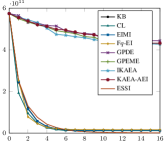
() $f_{1}$

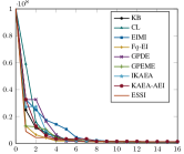
() $f_{3}$

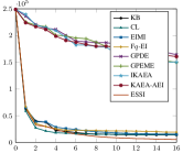
() $f_{4}$

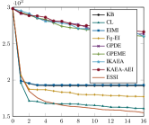
() $f_{5}$

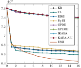
() $f_{6}$

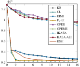
() $f_{7}$

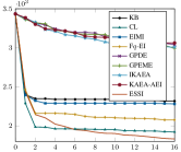
() $f_{8}$

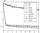
() $f_{9}$

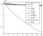
() $f_{10}$

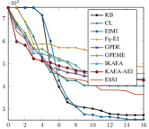
() $f_{11}$

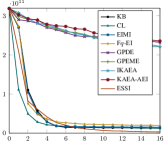
() $f_{12}$

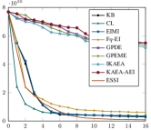
() $f_{13}$

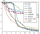
() $f_{14}$

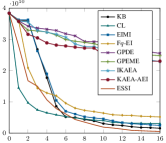
() $f_{15}$

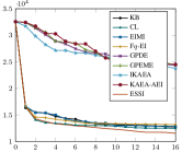
() $f_{16}$

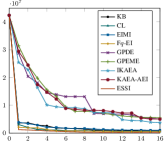
() $f_{17}$

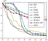
() $f_{18}$

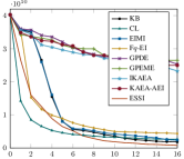
() $f_{19}$

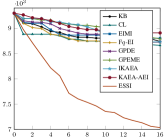
() $f_{20}$

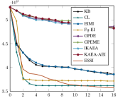
() $f_{21}$

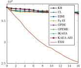
() $f_{22}$

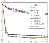
() $f_{23}$

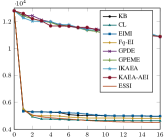
() $f_{24}$

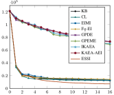
() $f_{25}$

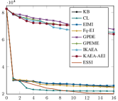
() $f_{26}$

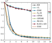
() $f_{27}$

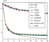
() $f_{28}$

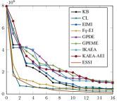
() $f_{29}$

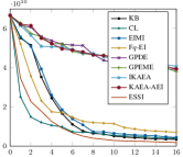
() $f_{30}$

Figure 7: Convergence plots of the compared batch approaches on the test problems as $q=64$.

Another interesting phenomenon can be seen from the convergence curves is that our ESSI converges slower than the four compared batch BOs at the beginning of iterations, but converges faster as the iteration goes on, and achieves better results at the end of iterations. The compared batch BO algorithms locate the acquisition samples in the original design space but our proposed ESSI algorithm finds acquisition samples in low-dimensional subspaces. Therefore, the compared batch BO algorithms are able to find better solutions at the beginning of iterations by searching over the whole design space. As the iteration goes on, most of the promising areas have been explored, further searching over the design space becomes less beneficial. In comparison, the proposed ESSI is able to continually find good solutions by searching in different low-dimensional subspaces. Therefore, it is able to find better solutions at the end of iterations.

At last, we compare the running time of these batch algorithms. The average running time of the compared algorithms is plotted in Fig. 8. Clearly, the four SAEAs are much faster than the five batch BOs. To select new points for expensive evaluations, the SAEAs only need to rank the individuals based on the acquisition function but the batch BOs need to optimize the acquisition function using the genetic algorithm. Therefore, the SAEAs need much fewer time to select individuals for expensive evaluation than the batch BOs. This is an advantage of SAEAs over batch BOs.

As the batch size $q$ increases, the computational time for selecting query points increases for the batch BO approaches, but the number of iterations decreases since the total function evaluations is fixed. Therefore, the total computational time for the batch BOs does not change much as $q$ increases from $4$ to $64$. Compared with the four batch BOs, our proposed ESSI approach is much faster. One reason is the our proposed approach selects query points in subspaces, therefore it is faster to solve the acquisition optimization problems. Another reason is that our proposed approach is able to solve the acquisition optimization problems simultaneously, therefore the computational time can be further reduced by using parallel computing.

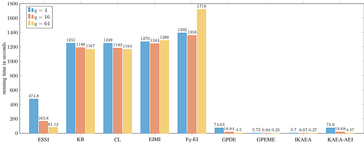
Figure 8: Running time of the compared batch approaches on the test problems.

V Conclusion

Extending Bayesian optimization to parallel computing is interesting and meaningful task. In this work, we propose a novel idea to develop batch Bayesian optimization algorithms. Different from existing methods, the newly proposed expected subspace improvement (ESSI) approach tries to select multiple query points in multiple subspaces. After getting a batch of points, we can then evaluate them in parallel. The proposed ESSI approach has no additional parameter, is easy to understand and simple to implement. The proposed ESSI approach has shown very competitive performances in both computational cost and optimization efficiency when compared with the standard Bayesian optimization and eight batch approaches through numerical experiments. However, our work does not consider expensive constraints and multiple expensive objective functions. Therefore, extending this idea to expensive constrained optimization and expensive multiobjective optimization might be interesting for future research.

References

- [1] J. Mockus, “Application of bayesian approach to numerical methods of global and stochastic optimization,” Journal of Global Optimization, vol. 4, no. 4, pp. 347–365, 1994.
- [2] D. R. Jones, M. Schonlau, and W. J. Welch, “Efficient global optimization of expensive black-box functions,” Journal of Global Optimization, vol. 13, no. 4, pp. 455–492, 1998.
- [3] J. Snoek, H. Larochelle, and R. P. Adams, “Practical bayesian optimization of machine learning algorithms,” in Advances in Neural Information Processing Systems, 2012, Conference Proceedings, pp. 2951–2959.
- [4] D. J. Lizotte, T. Wang, M. H. Bowling, and D. Schuurmans, “Automatic gait optimization with gaussian process regression,” in Proceedings of the 20th international joint conference on Artifical intelligence, vol. 7, 2007, Conference Proceedings, pp. 944–949.
- [5] R. Lam, M. Poloczek, P. Frazier, and K. E. Willcox, “Advances in bayesian optimization with applications in aerospace engineering,” in 2018 AIAA Non-Deterministic Approaches Conference, 2018, Conference Proceedings, p. 1656.
- [6] B. Shahriari, K. Swersky, Z. Wang, R. P. Adams, and N. d. Freitas, “Taking the human out of the loop: A review of bayesian optimization,” Proceedings of the IEEE, vol. 104, no. 1, pp. 148–175, 2016.
- [7] X. Wang, Y. Jin, S. Schmitt, and M. Olhofer, “Recent advances in bayesian optimization,” ACM Computing Surveys, vol. 55, no. 13s, p. Article 287, 2023.
- [8] H. Kushner, “A new method of locating the maximum point of an arbitrary multipeak curve in the presence of noise,” Journal of Basic Engineering, vol. 86, no. 1, pp. 97–106, 1964.
- [9] D. D. Cox and S. John, “A statistical method for global optimization,” in IEEE international conference on systems, man, and cybernetics, 1997, Conference Proceedings, pp. 1241–1246.
- [10] M. Schonlau, “Computer experiments and global optimization,” Thesis, University of Waterloo, 1997.
- [11] D. Ginsbourger, R. Le Riche, and L. Carraro, Kriging Is Well-Suited to Parallelize Optimization, ser. Adaptation Learning and Optimization. Springer Berlin Heidelberg, 2010, vol. 2, book section 6, pp. 131–162.
- [12] C. Chevalier and D. Ginsbourger, Fast Computation of the Multi-Points Expected Improvement with Applications in Batch Selection, ser. Lecture Notes in Computer Science. Springer Berlin Heidelberg, 2013, vol. 7997, book section 7, pp. 59–69.
- [13] S. Marmin, C. Chevalier, and D. Ginsbourger, “Differentiating the multipoint expected improvement for optimal batch design,” in International Workshop on Machine Learning, Optimization and Big Data, ser. Lecture Notes in Computer Science, P. Pardalos, M. Pavone, G. M. Farinella, and V. Cutello, Eds., vol. 9432. Springer International Publishing, 2015, Conference Proceedings, pp. 37–48.
- [14] J. Wang, S. C. Clark, E. Liu, and P. I. Frazier, “Parallel bayesian global optimization of expensive functions,” Operations Research, vol. 68, no. 6, pp. 1850–1865, 2020.
- [15] D. Zhan, Y. Meng, and H. Xing, “A fast multipoint expected improvement for parallel expensive optimization,” IEEE Transactions on Evolutionary Computation, vol. 27, no. 1, pp. 170–184, 2023.
- [16] J. Gonzalez, Z. Dai, P. Hennig, and N. Lawrence, “Batch bayesian optimization via local penalization,” in Artificial Intelligence and Statistics, 2016, Conference Proceedings, pp. 648–657.
- [17] Z. Li, S. Ruan, J. Gu, X. Wang, and C. Shen, “Investigation on parallel algorithms in efficient global optimization based on multiple points infill criterion and domain decomposition,” Structural and Multidisciplinary Optimization, vol. 54, no. 4, pp. 747–773, 2016.
- [18] D. Zhan, J. Qian, and Y. Cheng, “Pseudo expected improvement criterion for parallel ego algorithm,” Journal of Global Optimization, vol. 68, no. 3, pp. 641–662, 2017.
- [19] B. Bischl, S. Wessing, N. Bauer, K. Friedrichs, and C. Weihs, MOI-MBO: Multiobjective Infill for Parallel Model-Based Optimization, ser. Lecture Notes in Computer Science. Springer International Publishing, 2014, vol. 8426, book section 17, pp. 173–186.
- [20] Z. W. Feng, Q. B. Zhang, Q. F. Zhang, Q. G. Tang, T. Yang, and Y. Ma, “A multiobjective optimization based framework to balance the global exploration and local exploitation in expensive optimization,” Journal of Global Optimization, vol. 61, no. 4, pp. 677–694, 2015.
- [21] Q. Zhang and H. Li, “MOEA/D: A multiobjective evolutionary algorithm based on decomposition,” IEEE Transactions on Evolutionary Computation, vol. 11, no. 6, pp. 712–731, 2007.
- [22] W. Lyu, F. Yang, C. Yan, D. Zhou, and X. Zeng, “Batch bayesian optimization via multi-objective acquisition ensemble for automated analog circuit design,” in International Conference on Machine Learning, 2018, Conference Proceedings, pp. 3312–3320.
- [23] T. Robič and B. Filipič, “DEMO: Differential evolution for multiobjective optimization,” in International Conference on Evolutionary Multi-Criterion Optimization, 2005, Conference Proceedings, pp. 520–533.
- [24] J. Chen, F. Luo, G. Li, and Z. Wang, “Batch bayesian optimization with adaptive batch acquisition functions via multi-objective optimization,” Swarm and Evolutionary Computation, vol. 79, p. 101293, 2023.
- [25] Y. Jin, H. Wang, T. Chugh, D. Guo, and K. Miettinen, “Data-driven evolutionary optimization: An overview and case studies,” IEEE Transactions on Evolutionary Computation, vol. 23, no. 3, pp. 442–458, 2019.
- [26] P. I. Frazier, “A tutorial on bayesian optimization,” 2018. [Online]. Available: https://arxiv.org/abs/1807.02811
- [27] C. E. Rasmussen and C. K. Williams, Gaussian processes for machine learning. The MIT Press, Cambridge, MA, USA, 2006.
- [28] P. I. Frazier, W. B. Powell, and S. Dayanik, “A knowledge-gradient policy for sequential information collection,” SIAM Journal on Control and Optimization, vol. 47, no. 5, pp. 2410–2439, 2008.
- [29] P. Frazier, W. Powell, and S. Dayanik, “The knowledge-gradient policy for correlated normal beliefs,” INFORMS Journal on Computing, vol. 21, no. 4, pp. 599–613, 2009.
- [30] P. Hennig and C. J. Schuler, “Entropy search for information-efficient global optimization,” Journal of Machine Learning Research, vol. 13, no. Jun, pp. 1809–1837, 2012.
- [31] J. M. Hernández-Lobato, M. W. Hoffman, and Z. Ghahramani, “Predictive entropy search for efficient global optimization of black-box functions,” in Advances in neural information processing systems, vol. 27, 2014, Journal Article.
- [32] D. Zhan and H. Xing, “Expected improvement for expensive optimization: a review,” Journal of Global Optimization, vol. 78, no. 3, pp. 507–544, 2020.
- [33] D. Zhan, “Expected coordinate improvement for high-dimensional bayesian optimization,” Swarm and Evolutionary Computation, vol. 91, p. 101745, 2024.
- [34] N. Awad, M. Ali, J. Liang, B. Qu, and P. Suganthan, “Problem definitions and evaluation criteria for the CEC special session and competition on single objective real-parameter numerical optimization,” Nanyang Technological University, Singapore, Jordan University of Science and Technology, Jordan and Zhengzhou University, Zhengzhou China, Tech. Rep., 2017.
- [35] B. Liu, Q. Zhang, and G. G. E. Gielen, “A gaussian process surrogate model assisted evolutionary algorithm for medium scale expensive optimization problems,” IEEE Transactions on Evolutionary Computation, vol. 18, no. 2, pp. 180–192, 2014.
- [36] D. Zhan and H. Xing, “A fast kriging-assisted evolutionary algorithm based on incremental learning,” IEEE Transactions on Evolutionary Computation, vol. 25, no. 5, pp. 941–955, 2021.
- [37] D. Zhan, Y. Gui, and T. Li, “An anisotropic expected improvement criterion for kriging-assisted evolutionary computation,” in IEEE Congress on Evolutionary Computation, 2023, Conference Proceedings, pp. 1–8.