Phase Selection and Analysis for Multi-frequency Multi-user RIS Systems Employing Subsurfaces in Correlated Ricean and Rayleigh Environments
Abstract
We analyse the performance of a reconfigurable intelligent surface (RIS) aided system where the RIS is divided into subsurfaces. Each subsurface is designed specifically for one user, who is served on their own frequency band. The other subsurfaces (those not designed for this user) provide additional uncontrolled scattering. We derive the exact closed-form expression for the mean signal-to-noise ratio (SNR) of the subsurface design (SD) when all channels experience correlated Ricean fading. We simplify this to find the mean SNR for line-of-sight (LoS) channels and channels experiencing correlated Rayleigh fading. An iterative SD (ISD) process is proposed, where subsurfaces are designed sequentially, and the phases that are already set are used to enhance the design of the remaining subsurfaces. This is extended to a converged ISD (CISD), where the ISD process is repeated multiple times until the SNR increases by less than a specified tolerance. The ISD and CISD both provide a performance improvement over SD, which increases as the number of RIS elements (N) increases. The SD is significantly simpler than the lowest complexity multi-user (MU) method we know of, and despite each user having less bandwidth, the SD outperforms the existing method in some key scenarios. The SD is more robust to strongly LoS channels and clustered users, as it does not rely on spatial multiplexing like other MU methods. Combined with the complexity reduction, this makes the SD an attractive phase selection method.
Index Terms:
Reconfigurable Intelligent Surface (RIS), array signal processing, correlated Ricean and Rayleigh fadingI Introduction
Reconfigurable Intelligent Surfaces (RIS) are the focus of considerable research interest for next generation mobile communications, due to their ability to manipulate the wireless channel with minimal power consumption. RIS can enhance several aspects of system perfomance, including signal-to-noise-ratio (SNR), rank deficiency and blockage avoidance [1]. There is now a significant body of work on RIS, including design, testbeds, and performance analysis [2]. Standards development is also underway, with ETSI releasing its first report on RIS in 2023 [3].
Typical RIS implementations involve large numbers of elements, , in an array, where each element can be set to control the phase of the reflected signal. A key challenge is selecting the RIS element reflection coefficients to maximise the total SNR at the target receiver. An analytically determined optimal RIS design does not appear feasible for a multi user (MU) system. Iterative schemes have been designed [4, 5, 6, 7], but have high computational complexity. In order to keep power consumption low, limited processing can be done on the RIS itself. In addition, these methods demand significant amounts of channel state information (CSI) and necessitate complex receiver processing. Typically, the matrix operations required are similar to those for minimum mean squared error (MMSE) receivers. Therefore, while they may perform well, these methods would be challenging to implement.
Complexity reduction research in RIS design includes using statistical CSI, such as in the codebook designs in [8], and the study of the trade off between energy efficiency and spectral efficiency in [9]. In terms of using channel estimates, lower complexity has been achieved for both a double RIS system [10] and a discrete phase shift system [11]. While both considerably reduce overall computation, they target high performance. This necessitates iterative optimisation and repeated matrix operations (inversion or singular value decomposition (SVD)). In this paper, we take a different direction to these works, targeting useful (but not near-optimal) performance improvements for the RIS while keeping the RIS design and receiver processing remarkably simple.
In [12], we proposed a low complexity subsurface design (SD) where a RIS of elements is divided into subsurfaces with elements, respectively, where is the number of users. Each user operates on a different frequency, so that matched filtering (MF) can be used at the receiver, and one subsurface is designed per user. The elements designed for a specific user are selected using the optimal single user (SU) phase selection method proposed in [13]. The elements designed for other users provide uncontrolled scattering for this user. This may assist the user, particularly in higher frequency systems where there is little natural uncontrolled scattering in the environment. As elements are only being designed for one of users, channel estimation is reduced by a factor of . The use of MF ensures that the receiver processing is as simple as possible. Note that simple beamforming is more practical at higher frequencies and thus SU systems remain of strong interest in 5G [14].
In our preliminary work in [12], we only considered the performance of the SD for a line-of-sight (LoS) RIS-base station (BS) channel and correlated Rayleigh user equipment (UE)-BS and UE-RIS channels. In reality, it is likely that all channels will have both LoS and non-line-of-sight (NLoS) components. Therefore, we now significantly extend our work by investigating the performance of this simple and practical method for more general and realistic correlated Ricean fading channels. This versatile analytical tool can be simplified to more specific combinations of LoS and NLoS channels as desired. We also extend the subsurface design to a low complexity iterative subsurface design (ISD). The SD assumes that each subsurface is designed independently with no knowledge of phases set for other users. The ISD sets the subsurfaces sequentially from the weakest to strongest user, utilising the knowledge of all phases set for other users to improve the design. Thus, users with the largest impact on total SNR benefit from the most prior knowledge. The ISD sees this process performed once, but it can be performed repeatedly until it converges and the total SNR stops increasing. This is referred to as the converged ISD (CISD). The ISD and CISD offer performance improvements while still benefiting from relatively low computational complexity and a simple MF receiver.
Using analysis and simulations, we both verify the accuracy of our derivation and investigate the performance of the SD and ISD. The mean SNR of both methods is compared for a range of RIS dimensions. The mean sum rate supported by the SD is compared to a lowerbound benchmark equivalent to no channel knowledge (e.g. randomly selected RIS phases) and the MU method in [4]. This was selected for comparison as it is the lowest complexity existing full MU design that we are aware of, and while other methods may offer better performance, it is highly probable that they will require considerably higher system complexity. The impact of a range of system parameters is considered including Ricean K-factor, correlation and array dimensions.
Notation: Upper and lower boldface letters represent matrices and vectors, respectively. We define vector , where is the -th block of vector and is the -th element of the -th block. is a matrix comprising of submatrices, or blocks. is the -th element of the -th block across and -th block down. Matrices are indexed this way except where explicitly defined otherwise in the text. denotes a matrix relating to user . is the set of complex numbers. is the Real operator. represents a complex Gaussian distribution with mean and covariance matrix . represents statistical expectation. , and represent the transpose, conjugate and Hermitian transpose operators, respectively. The angle of a vector, , of length is denoted as and the exponent as . is the Euclidean norm. is the confluent hypergeometric function and is the Gaussian hypergeometric function. denotes a Laguerre function of non-integer degree . is the complete gamma function. is the probability density function (PDF) of a complex random variable , and is the joint PDF of complex random variables and . is the -th order Bessel function of the first kind and is the -th order modified Bessel function of the first kind.
II System Model
We consider an uplink RIS aided system, as shown in Fig. 1, consisting of a RIS panel with N elements and a BS with M antennas. K single-antenna users are located in the vicinity of the BS and RIS. A RIS link (UE - RIS - BS) and a direct link (UE - BS) connect the UE to the BS. The system bandwidth, , is split into bands of Hz, with one user per band. The phase response of the RIS, and therefore the phase shift in the reflected signal, is fixed across the frequency bands. The RIS elements are grouped into “subsurfaces” and each subsurface is designed for a different user.
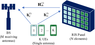
For user in band , let , and be the direct, UE-RIS and RIS-BS channels, respectively. is a diagonal matrix of reflection coefficients for the RIS which can be given in block diagonal form, where the -th block is designed to enhance the channel for user . , where . is the number of RIS elements chosen to support user and . The received signal in band at the BS is
| (1) |
where is the signal being sent from user , , and is additive white Gaussian noise. Using the block diagonal form of , (1) becomes
| (2) |
where , , and .
II-A Channel Model
For this work, we consider correlated Ricean channels consisting of a rank-1 LoS and correlated Rayleigh component for all links. The LoS components are comprised of steering vectors and the scattered components adopt the Kronecker correlation model. Therefore, the channels for user are
| (3) | ||||
| (4) | ||||
| (5) |
with
and where , and are the channel gains, , and are the Ricean K-factors, , and are the LoS channel components for the th user and , and are the scattered channel (SC) components for the th user. Here,
where is the steering vector of the LoS ray for the direct link at the BS, and are steering vectors for the LoS ray for the RIS-BS link at the BS and RIS, respectively, and is the steering vector of the LoS ray for the UE-RIS link at the RIS. , , and are the correlation matrices for the RIS-BS link at the BS and RIS ends, the UE-BS link and UE-RIS link, respectively, and and are all matrices and vectors containing independent and identically distributed entries.
III Phase Selection Methods
Partitioning the RIS elements into subsurfaces and independently designing each subsurface for one user allows for low complexity and effective RIS phase selection methods, which is especially important for the high frequency environments it is envisaged RIS will be used in. This section outlines three methods that utilise these principles: a simple approach that uses the SU optimal phase selection method for when is rank-1, a sub-optimal extension of this for when has a scattered component, and a higher-performing but more complex iterative version.
III-A LoS Phase Selection Method
As we first proposed in [12], the phases of a subsurface designed for the -th user can be set according to the SU method set out in [13], so that
| (12) |
where
| (13) |
The phases set for each user are optimal for that user when is purely LoS, and close to optimal when has a strong LoS component. This method leads to a -fold reduction in the required CSI compared to typical RIS designs, due to only requiring the estimation of rather than channel elements per user. There are no complex matrix operations required and a simple MF receiver can be used. These advantages make this approach a very attractive option for implementation.
III-B Extended Subsurface Design for NLoS Systems
The design in (12) and (13) works well for strongly LoS channels. However, if there is a strong scattered component, a different approach provides better results. As there is no optimal closed form SU phase selection method when is not rank 1, we propose the following adaptation to the method outlined in Sec. III-A. As we proposed in [12], we take the singular value decomposition of , so that , where , and the singular values are . The strongest rank 1 component of is , where and are the leading left and right singular vectors, respectively. This has the same structure as a pure LoS channel, so the same design can be used by considering just the strongest component, giving,
| (14) |
where
| (15) |
III-C Iterative Phase Alignment
The subsurface methods outlined in Secs. III-A and III-B select phases to maximise the norm of the subsurface’s RIS link, , and then rotate these phases to align with the non-RIS-controlled direct link, . It is assumed that each subsurface is designed independently, with no knowledge of any phases that have been set for other users. If we assume that the subsurfaces are set sequentially, we can improve these methods by treating previously set subsurfaces as fixed channels. After selecting phases to maximise the RIS link, they can be rotated to align with a combination of the direct path and the RIS paths that have already been set for other UEs. This is done by including this information into (LoS case) or (NLoS case). The subsurfaces are set from the weakest UE-RIS channel to the strongest, so that the most impactful channels can benefit from the most information. This process is detailed in Algorithm 1, where index refers to a function that returns the index of elements in a list and sort refers to a function that reorders elements of a list from smallest to largest.
This iterative method improves mean SNR as shown in Sec. V-A at the cost of a significant increase in CSI requirements at the BS. contains channel elements, with corresponding to those impacted by a specific subsurface. The iterative method requires the computation of the magnitude of a user’s UE-RIS link to rank channels based on their impact, so knowledge of the amplitude of all channel elements is required. In contrast, the methods in Secs. III-A and III-B only consider the impact on a user from each subsurface, so only the subsurface specific elements are required. The benefits of the iterative method vary depending on channel conditions such as correlation and link power, as will be shown in Section V-A.
IV Analysis
In this section, we focus on an analysis of the mean SNR as prior work [13, 12, 18] has shown it to be tractable, to provide tight rate bounds via and to deliver system insights. In particular, we derive the mean SNR for a correlated Ricean environment, where , and all consist of a rank-1 LoS and a scattered component. We consider the important case where has a strong, but not pure, LoS component. This leads to a stable, slow moving RIS-BS channel, allowing the SD to be used and achieve close to optimal performance for a given subsurface [19]. Therefore, in (12) is used in this section. This general case will then be simplified to two special cases where and are correlated Rayleigh channels; in the first is correlated Ricean, and in the second it is a rank-1 LoS channel.
IV-A Mean SNR for Correlated Ricean Systems
We now consider the mean value of each term in (19) to calculate for correlated Ricean systems. From [19],
| (20) |
and
| (23) |
All remaining terms are derived in Appendix A and their results are listed below.
| (26) |
where
| (29) |
| (30) |
where is given in (29), and, dropping subscripts for readability, and .
| (33) |
where
| (34) |
| (35) |
, , and .
IV-B Special Case 1: Mean SNR for Correlated Ricean with Correlated Rayleigh UE Channels
Now consider the subcase where is correlated Ricean and the UE channels are correlated Rayleigh.
Assuming and are correlated Rayleigh channels, then . As and are independent, and and are independent for , and contain zero-mean terms. Therefore, (19) simplifies to
| (39) |
The result for is the same as (20), while (23), (33) and (36) no longer rely on UE link K-factors and can be simplified to
| (40) |
| (43) |
| (46) |
IV-C Special Case 2: Mean SNR for LoS with Correlated Rayleigh UE Channels
Now consider the further simplification of for LoS and correlated Rayleigh UE links.
IV-D Insights from Analysis
From the analysis, the following insights are drawn. Equations (20) - (26), (30) (33) and (36) demonstrate the obvious properties that SNR improves with an increase in the number of RIS elements per user, BS elements and/or channel gain.
Both (33) and (36) include a Gaussian hypergeometric function, which increases monotonically with the final argument. The final arguments of both terms increase as the RIS spatial channel correlation increases, which occurs when RIS elements are placed closer together. In contrast, higher element spacing at the BS increases rate, due to the component of (23). If elements are spaced too close together at the BS, this term decreases, as is shown in [13]. However, as the terms in (33) and (36) are quadratic, and thus typically the largest, a change in spatial correlation at the RIS is more influential to the overall SNR than a change in spatial correlation at the BS.
Therefore, the mean SNR is improved by typical factors such as large system dimensions and channel gain, and by the less obvious channel features of an uncorrelated channel and a highly correlated channel.
V Numerical Results
Numerical results were generated to verify the analysis above and explore the performance of the subsurface design. The channel gain values are selected based on the distance based path loss model detailed in [15], where
| (52) |
is the reference distance of 1 m, is the pathloss at (-30 dB), is the link distance in metres and is the pathloss exponent (, and ).
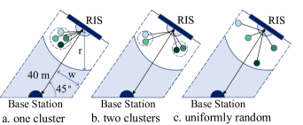
It is assumed that the RIS is fixed at 40 m away from the BS, at an angle of rad. Users are then dropped in a straight corridor of width between BS and RIS, at a maximum distance of from the RIS with an exclusion zone of 1 m around the RIS. This region ensures that the path from the UE through the RIS significantly contributes to the total channel, and the effects of the RIS can be clearly seen. User clusters are considered to investigate the effect of people naturally congregating. Three types of user grouping were used in simulations. As seen in Fig. 2, layout A places all users in one cluster, where they are all in the same area spaced 1 m apart and layout B creates 2 clusters of users, with users spaced 1 m apart. Cluster locations are drawn from a uniform distribution. Layout C places each user randomly within the corridor, again using a uniform distribution. To ensure that results are general and not tied to a specific UE location, random user drops are generated per layout, each with replicates.
For simulation purposes, we use the Rayleigh fading correlation model proposed in [21], where
| (53) |
, is the Euclidean distance between BS antennas/RIS elements and , measured in wavelength units, and is the number of BS antennas/RIS elements.
The steering vectors , , and correspond to the vertical uniform rectangular array (VURA) model and are given in [22]. Elements are arranged in a VURA at intervals of and wavelengths at the BS and RIS, respectively. and are the number of BS and RIS elements per row and and are the number of BS and RIS elements per column, such that and . and are the elevation and azimuth angles of departure (AoDs) at the RIS and and are the corresponding elevation and azimuth angles of arrival (AoAs) at the BS. We assume the RIS is on a rad angle with respect to the BS, so rad and rad. We also assume both are at the same height, so rad.
Without loss of generality we assume and is selected in Sec V-A so that the mean output SNR for one UE is 5 dB in a system using the SD where , , , and . In Sec V-B, we select so that the mean output SNR for one UE is 5 dB in a system using the SD where , , , , and the RIS-BS channel is purely LoS, an important special case. These parameter values and definitions do not change throughout the results, unless specified otherwise.
V-A Mean SNR Comparison of Subsurface Methods in Sec. III
Fig 3 verifies the analytical results in Sec IV-A by showing the equivalence of and the simulated mean SNR for the SD, and then compares this with the simulated mean SNR for the ISD. Two versions of the ISD were implemented. The first iterates through all subsurfaces once, as shown in Sec III-C. The second iterates through all subsurfaces and calculates the SNR of the system. It then repeats this process multiple times until the SNR of the system has converged, i.e. it increases by less than a specified tolerance from one iteration to the next. For these simulations, the tolerance was specified to be . We will refer to this method as the converged ISD (CISD).
The array parameters for Fig. 3 are , , , and all K-factors are 1. Larger spacings between the RIS elements ( rather than ) were used here to highlight the performance differences of the methods. Higher correlation leads to greater similarity in the SNR per user of the SD and CISD, as discussed below.
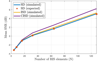
It can be seen that the simulated mean SNR for the method outlined in Sec III-A is virtually indistinguishable from the derived in Sec. IV-A, verifying that result. As expected, the mean SNR for all 3 methods increases with , however the rate of improvement decreases as increases. This is expected, as it is well known that the RIS SNR can grow quadratically with [13] so that the dB relationship is logarithmic. The quadratic behaviour can be seen in (33), (43), and (48) where the term contains the sum of positive terms, giving a contribution of . The ISD and converged ISD both provide more benefit at higher . At high , more improvement can be made by iterating, as there are more elements to vary and hence more opportunities to improve the performance of the system. This improvement is more pronounced when the correlation between RIS elements is lower, as discussed below. The mean SNR for a range of at both RIS element spacings of and is shown below in Table I. The ISD performs better when correlation is lower. This may be due to the fact that there is more variability in the previously set subsurfaces creating the fixed channels for the iterative design. Hence, less correlation causes increased variation in the fixed channels which the iterative design can make use of.
| N | Mean SNR (dB) | |||
|---|---|---|---|---|
| SD | CISD | SD | CISD | |
The increase in performance provided by the ISD and CISD also leads to an increase in required CSI. Both methods require the same amount of CSI as each needs to estimate channels between the RIS and the UE, as opposed to the required by the SD. This is due to the need to measure the impact of each subsurface on all users, rather than on just the user it is designed for. Gathering CSI is expected to be challenging for RIS systems, so the benefit from an iterative method would need to be weighed up against this additional CSI requirement.
Each iteration of the ISD is very simple. Additional complex multiplies are needed to compute channel norms to order subsurfaces by impact and to recalculate fixed channel components. For the CISD, the SNR also needs to be computed each iteration. Table II compares the complexity of the three subsurface methods if iterations are required.
| SD | ISD | CISD | |
|---|---|---|---|
| Multiplies | |||
| Divides | |||
| Mathematical Functions | None | 1 sort() | |
| 1 index() | 1 sort()
1 index() |
||
| Array | |||
| Functions | None | 1 sort() | |
| 1 index() | 1 sort()
1 index() |
The average number of iterations required for convergence for each is shown in Table III. The largest mean number of iterations for an , system occurs when and is 6.60. In this scenario, when the maximum number of iterations is fixed at 7, the resulting SNR averages to be 99.8% of the fully converged SNR. Hence, restricting the number of iterations to a fixed amount has little impact on performance.
| N | Mean number of iterations | |
|---|---|---|
| 2.40 | 2.35 | |
| 2.65 | 2.56 | |
| 2.96 | 2.96 | |
| 3.50 | 3.96 | |
| 4.12 | 5.04 | |
| 5.42 | 6.60 | |
V-B Mean Sum Rate of SD versus Non-Subsurface Methods
Many existing MU RIS phase selection methods, such as those in [5, 6, 7], focus on achieving near optimal performance. Necessarily, they have challenging computational complexity requirements. The lowest complexity MU method we are aware of is that first proposed in [4]. While other methods may offer better performance, the design in [4] is more likely to be considered for practical implementation. This method approximately minimises the total mean squared error (TMSE) of a MMSE receiver. All users are placed in one band, so each user has times the bandwidth (BW) when compared to users served by the SD. In [12], we compared the SD and TMSE method in terms of BW, complexity and fairness. The SD offers a reduction in complex multiplies by a factor of , requires no matrix operations, provides fairer results according to Jain’s fairness test, uses a much simpler receiver type (MF vs MMSE) and reduces CSI requirements by a factor of . Hence, even when compared to the simplest RIS designs, the SD approach offers substantial complexity savings.
In this section, the mean sum rates for the SD and TMSE methods are compared with the mean sum rate for randomly selected phases. The inclusion of random phases creates a lower bound to compare both methods against. For the random approach, the phase shift of each element is generated from a uniform distribution between 0 and . It is assumed that all users are in one frequency band like the TMSE example. We investigate the impact of important system features, such as K-factor levels, correlation, system size and user locations.
V-B1 K-Factors and Clustering
Figs. 4, 5 and 6 compare the mean sum rate for the SD with that of random phases and the TMSE design for varying levels of the UE-BS, RIS-BS and UE-RIS K-factor, respectively. , as defined in (LABEL:eq:etad), (LABEL:eq:etarb) and (LABEL:eq:etaur), rather than K-factor itself is plotted so the proportion of the link that is LoS can be easily observed.
The array parameters for Figs. 4, 5 and 6 are , , , , , , and . The two K-factors not being varied in each plot are set to 1 so that the LoS and NLoS component strengths are equal. The coloured lines designate the type of RIS design, while line types (given in black in the legend) designate the user locations.
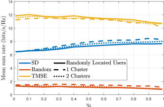
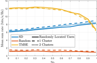
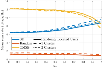
It can be seen in Figs. 4, 5 and 6 that despite the significant BW restriction on the SD, there are still operating scenarios where it achieves higher rates than the TMSE design for significantly lower complexity. It is also clear that a more dominant LoS link is beneficial for the SD, but negatively impacts the TMSE design. As the K-factor, and therefore (as defined in (LABEL:eq:etad), (LABEL:eq:etarb) and (LABEL:eq:etaur)) of a channel increases, the rank of that channel decreases until it reaches rank-1 when . This limits the spatial multiplexing ability of the channel by reducing diversity. Insufficient diversity leads to the inability to separate MU channels. As all users are in separate bands for the SD, a lack of channel diversity is not an issue. The SNR improves as channels can be aligned so that more power is directed towards the user as the rank decreases. However, for the TMSE design where all users are located in one frequency band, the inability to separate channels as the K-factor increases leads to a significant drop in rate. A slight exception to this trend can be seen in Fig. 5 between and . Note that the TMSE method assumes a LoS component in , so increasing the K-factor when is low helps slightly, as the channel becomes more similar to that which the framework was built upon. However, above this threshold, the reduction in diversity dominates and the overall rate reduces. The inability to separate channels also negatively impacts the random design, but this impact is lower as it is already operating at a low rate.
Varying the K-factors for the UE-RIS and RIS-BS channels results in similar mean sum rate behaviour. Data through the RIS must travel through both channels, so changing the diversity of one places limits on the other, and thus on the whole RIS link. This is particularly prominent when the LoS link is dominant - the mean sum rate for the TMSE method drops dramatically, due to the direct link providing the only diversity. The same can be observed for the random method, but to lesser extent. In comparison, when the UE-BS channel becomes strongly LoS, the mean sum rate for the TMSE design is less impacted. As discussed at the start of Sec. V, UEs are dropped in locations that ensure a strong RIS path, to ensure the effects of the RIS are visible. Therefore, the rate remains high in this case due to the strong RIS link being unaffected.
The impact of placing all 4 users in a cluster (layout A) is most noticeable in strongly LoS channels, where it improves the rate of the SD and lowers the rate of the TMSE method. Clustering users reduces channel diversity, and therefore negatively impacts the rate of the single frequency TMSE method. A key benefit of the SD is its robustness to clustered users, a realistic scenario in highly populated areas. As it does not rely on spatial multiplexing, clustered users improve its performance due to the similarity of the LoS paths, allowing those subsurfaces designed for other users to provide better signal enhancement. Interestingly, clustering also helps the random method. This is likely due to the fact that when the random phases happen to be beneficial for one user, they benefits all UEs in the cluster.
V-B2 Correlation
Fig. 7 compares the mean sum rate for the SD and TMSE designs for a range of element spacings at the RIS and BS. Elements located closer together result in higher correlation. The array parameters are the same as for Figs. 4-6, except for the varied element spacing.
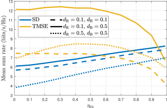
For the SD, it is observed that lower element spacing at the RIS increases rate. This verifies the analysis in Sec. IV-D, as (33) monotonically increases with correlation. In contrast, lower element spacing at the BS decreases rate. This also verifies findings in Sec. IV-D, as (23) decreases with correlation. The RIS element spacing is more influential than the BS element spacing to the rate of the SD. As expected, the rate is higher for the scenario where both spacings are than when both spacings are . This is due to RIS correlation predominantly affecting the typically larger quadratic term in (33), and BS correlation mostly affecting the typically smaller cross product in (23).
The TMSE method is designed for a RIS-BS channel with a strong LoS component, which is assisted by higher correlation and a higher . This is evidenced by smaller RIS element spacing increasing the mean sum rate of the TMSE design. However, as also becomes large, there is a substantial performance degradation. While the algorithm is more accurate for this scenario, strongly LoS channels are not ideal to support multiple users, as the MU channels cannot be separated within a single frequency band. Also, unlike the SD, the BS element spacing is more influential to the rate of the TMSE design. The TMSE method relies on channel separability to serve multiple users in one band. Decreasing the BS element spacing limits this in both the direct and RIS paths, significantly decreasing the performance of the TMSE method. The SD performs comparatively better when correlation is high at the BS, due to separability not being required for its operation.
V-B3 Array Dimensions
Fig. 8 compares the mean sum rate for 5 combinations of and values to investigate the impact of array dimensions. The array parameters are , , , and .
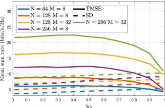
In the case of TMSE, it is observed that mean sum rate is influenced significantly more by than . The largest mean sum rates are for the cases, and then ordered by the size of . Comparatively, the cases give the smallest mean sum rates, with , performing the worst. The TMSE method needs sufficient to multiplex, as impacts both the direct and RIS links. While a higher is beneficial, it only affects the RIS link. Therefore, if is too low or is too high for efficient multiplexing in the RIS path, the direct path could still support it if is large enough. Table IV shows that the percentage decrease in the mean sum rate from to is greatest for the TMSE method when is large and is small.
| M | N | Mean sum rate decrease from to (%) |
| 8 | 256 | 56.2 |
| 32 | 256 | 49.6 |
| 8 | 128 | 45.6 |
| 32 | 128 | 40.0 |
| 8 | 64 | 29.4 |
In contrast, the mean sum rate of the SD increases slightly with and is much more robust in low scenarios, outperforming the TMSE method for all cases when . is the more influential parameter for the SD - the highest mean sum rates are from the highest scenarios, and ordered within these by the highest , which verifies the analysis in Sec. V. As the SD does not rely on multiplexing, is less important, and higher leads to more elements designed for each user and more scattering elements. A higher also leads to more power aligned in a specific direction and thus an increased mean sum rate. As percentage increase is a poor metric due to the small magnitude of the change, Table V shows the SD mean sum rate increase from to for each parameter set.
| M | N | Mean sum rate increase from to (bits/s/Hz) |
| 8 | 256 | 2.62 |
| 8 | 128 | 2.18 |
| 8 | 64 | 1.62 |
| 32 | 256 | 1.39 |
| 32 | 128 | 1.16 |
The mean sum rate increase for the SD is largest for small and large . Changing has no effect on the direct link. Therefore, when the direct link is weaker and the RIS link is stronger, a higher percentage of the total channel is being strengthened by the stronger LoS component in the RIS-BS channel. Therefore, the SD method has advantages at high and and low , where the TMSE method is weakest.
VI Conclusion
In this work, we extend the SD to a higher performing low complexity iterative method (ISD) by setting the subsurfaces sequentially from the weakest user to the strongest so that the users with the largest impact on total SNR benefit from the most prior knowledge. We then propose a converged ISD (CISD), where the ISD is repeated until the SNR increases by less than a specified threshold. We compared the performance of the SD, ISD and CISD, and found that the iterative methods outperform the SD. The most benefit from the CISD occurs at high where there are more elements that can be further improved with increased knowledge. We also derive the exact closed form expression for the mean SNR of the RIS SD where spatially correlated Ricean fading is assumed for all channels, leading to deeper insights into system performance. This is a very general analysis, and thus we show that the expression can be simplified to verify the results in [12] for correlated Rayleigh UE-BS and UE-RIS channels and a LoS RIS-BS channel. We showed that even while having significantly less BW per user, the SD outperformed the much more complex TMSE method for the realistic scenarios when a channel is strongly LoS or users are clustered together.
Appendix A Derivation of Mean SNR
We compute the mean SNR by taking the expectation of each term in (19). The first two terms, and , were derived in [19] with their results listed in (20) and (23). There are four remaining terms to derive. Term 1: As the scattered terms are uncorrelated and hence zero mean,
| Using the definitions for LoS terms in Sec. II-A, | ||||
| (91) | ||||
where is as given in 29 and derived in Appendix B. Term 2: Expanding out and gives
| (94) |
From (129) and (130) in Appendix B,
| (95) |
As is a correlated Ricean vector, we can write and , where and represent the LoS components, and represent the scaling of the scattered terms and . The Gaussian term of any element can be written as a scaled version of another with noise, so and , where represents noise and represents the spatial correlation between the elements. Returning to the standard channel definitions in (5) allows us to rewrite as
| (96) |
From (4.1) in [23],
| (97) |
Using the PDF for a complex random variable (RV) in (3.4) of [23] and letting , and ,
| (98) |
Using Euler’s formula and the difference of cosines relationship in (1.313.5) and then the integral result in (3.937.2) of [24], the inner integral can be evaluated to give
Rewriting the modified Bessel function as in (8.406.3) and integrating according to (6.631.1) in [24] gives
| (99) |
Therefore,
| (100) |
Expanding into the form seen in (4), taking the expectation of each term and removing zero mean cross products,
| (101) |
Finally, is defined in (29) and will be derived in Appendix B. Substituting (95), (100), (Appendix A Derivation of Mean SNR) and (29) into (94) gives (30). Term 3: Expanding out with split into LoS and scattered components (as seen in (4)) and taking the mean value leaves only the squared terms, due to the independence of the cross product terms. Hence,
| (102) |
Splitting into a sum of its terms, applying the same process as in (Appendix A Derivation of Mean SNR) for , replacing with its expanded form in (12) and simplifying gives
| (103) |
From [19],
| (104) |
where , , , , , and when as defined in [20].
can be found using the same process as for , giving
| (105) |
where
| (106) |
and the result from (104) is used for . Combining (103) and (105) gives (33).
Term 4: Splitting into two sums,
| (109) |
Rewriting as a sum of its terms and taking the expectation of each independent pair of terms gives
| (112) |
Following the procedure used for (Appendix A Derivation of Mean SNR),
| (113) |
Expanding out and simplifying the expression gives
| (114) |
where . Appendix C will derive , with the final result stated in (37). Expanding into the form seen in (5), taking the expectation of each term and removing the zero mean cross product terms gives
| (115) |
Combining (113), (114) and (115) gives (112). As for , rewriting as a sum of its terms and taking the expectation of each independent group gives
| (118) |
Again, from (Appendix A Derivation of Mean SNR),
| (119) |
As will be shown in Appendix B,
| (122) |
| (125) |
Finally, using the same process as for (115),
| (126) |
Therefore combining (119), (122), (125) and (126) gives (118), and combining (112) and (118) gives (109).
Appendix B Derivation of
Appendix C Derivation of
Let . Using the joint PDF for two complex RVs given in (24a) of [20],
Applying the variable transformations and ,
| (131) |
where , , , , , and .
We can now integrate with respect to both and . Rewriting and using Euler’s formula allows the double integral over the phases to be split into four smaller double integrals. Rewriting in the form seen in [24, 8.511.4] and the resulting in the form seen in [24, 1.313.5], removing periodic terms with zero-valued integrals, applying the product to sum formula found from [24, 1.313.5] and finally integrating each of the four double integrals using [24, 3.915.2], we get
| (132) |
where and when . To integrate with respect to and , we can rewrite the modified Bessel function as a Bessel function using [24, 8.406.3], expand that function to its series form using [24, 8.402] and integrate each integral using [24, 6.631.1], resulting in (37).
References
- [1] Q. Wu and R. Zhang, “Towards smart and reconfigurable environment: Intelligent reflecting surface aided wireless network,” IEEE Commun. Mag., vol. 58, no. 1, 2020.
- [2] Y. Liu et. al., “Reconfigurable intelligent surfaces: Principles and opportunities,” IEEE Commun. Surv. Tutor., vol. 23, no. 3, 2021.
- [3] European Telecommunications Standards Institute, “Reconfigurable intelligent surfaces (RIS); Communication models, channel models, channel estimation and evaluation methodology,” 2023. [Online]. Available: https://www.etsi.org
- [4] I. Singh et. al., “Efficient optimization techniques for RIS-aided wireless systems,” arXiv preprint, Sept. 2022.
- [5] S. Abeywickrama, R. Zhang, and C. Yuen, “Intelligent reflecting surface: Practical phase shift model and beamforming optimization,” IEEE ICC, 2020.
- [6] H. Gao et. al., “Robust beamforming for RIS-assisted wireless communications with discrete phase shifts,” IEEE Wireless Commun. Lett., vol. 10, no. 12, pp. 2619–2623, 2021.
- [7] S. Buzzi et. al., “RIS configuration, beamformer design, and power control in single-cell and multi-cell wireless networks,” IEEE Trans. Cogn. Commun. Netw., vol. 7, no. 2, pp. 398–411, 2021.
- [8] X. Jia et. al., “Environment-aware codebook for reconfigurable intelligent surface-aided MISO communications,” IEEE Wireless Commun. Lett., vol. 12, no. 7, pp. 1174–1178, 2023.
- [9] L. You et. al., “Energy efficiency and spectral efficiency tradeoff in RIS-aided multiuser MIMO uplink transmission,” IEEE Trans. Signal Process., vol. 69, pp. 1407–1421, 2021.
- [10] Q. Xue et. al., “Multi-user mmWave uplink communications based on collaborative double-RIS: Joint beamforming and power control,” IEEE Commun. Lett., vol. 27, no. 10, pp. 2702–2706, 2023.
- [11] J. An et. al., “Low-complexity channel estimation and passive beamforming for RIS-assisted MIMO systems relying on discrete phase shifts,” IEEE Trans. Commun., vol. 70, no. 2, pp. 1245–1260, 2022.
- [12] A. S. Inwood et. al., “Phase selection and analysis for multi-frequency multi-user RIS systems employing subsurfaces,” IEEE WCNC, 2023.
- [13] I. Singh, P. J. Smith, and P. A. Dmochowski, “Optimal SNR analysis for single-user RIS systems,” IEEE PIMRC, pp. 549–554, 2021.
- [14] D. Astely et. al., “Meeting 5G network requirements with massive MIMO,” Ericsson Technology Review, 2022.
- [15] Q. Wu and R. Zhang, “Intelligent reflecting surface enhanced wireless network via joint active and passive beamforming,” IEEE Trans. Wireless Commun., vol. 18, no. 11, pp. 5394–5409, 2019.
- [16] Q. U. A. Nadeem et. al., “Asymptotic max-min SINR analysis of reconfigurable intelligent surface assisted MISO systems,” IEEE Trans. Wireless Commun., vol. 19, no. 12, 2020.
- [17] M. A. Kishk and M. S. Alouini, “Exploiting randomly located blockages for large-scale deployment of intelligent surfaces,” IEEE J. Sel. Areas Commun., vol. 39, no. 4, 2021.
- [18] M. H. N. Shaikh et. al., “On the performance of dual RIS-assisted V2I communication under Nakagami-m fading,” in IEEE VTC2022-Fall, 2022.
- [19] I. Singh, P. J. Smith, and P. A. Dmochowski, “Optimal SNR analysis for single-user RIS systems in Ricean and Rayleigh environments,” IEEE Trans. Commun. Technol., pp. 9834–9849, 2022.
- [20] J. R. Mendes and M. D. Yacoub, “A general bivariate Ricean model and its statistics,” IEEE Trans. Veh. Technol., vol. 56, no. 2, pp. 404–415, 2007.
- [21] E. Björnson and L. Sanguinetti, “Rayleigh fading modeling and channel hardening for reconfigurable intelligent surfaces,” IEEE Wireless Commun. Lett., vol. 10, pp. 830–834, 2021.
- [22] C. Miller et. al., “Analytical framework for full-dimensional massive MIMO with ray-based channels,” IEEE J. Sel. Topics Signal Process., vol. 13, no. 5, pp. 1181–1195, 2019.
- [23] K. S. Miller, Complex Stochastic Processes: An Introduction to Theory and Application. Addison-Wesley, 1974, p. 76–100.
- [24] I. S. Gradshteyn and I. M. Ryzhik, Table of Integrals, Series and Products (Corrected and Enlarged Edition). Academic Press, 1980.
![[Uncaptioned image]](/html/2411.15965/assets/Amy.jpg) |
Amy S. Inwood (S’18) received the B.E (Hons.) degree in electrical and electronic engineering from Te Whare Wānanga o Waitaha University of Canterbury (UC), NZ, in 2021. She is pursuing her Ph.D. degree in electrical and electronic engineering, focusing on the statistical analysis of RIS-aided wireless communication systems. Her research interests include statistical analysis, 5G-6G wireless communications and RIS and other multi-antenna systems. She served as the Chairperson of the IEEE Student Branch (New Zealand South Section) in 2020 and the Postgraduate Representative 2021 - 2023. |
![[Uncaptioned image]](/html/2411.15965/assets/PSmith.jpg) |
Peter J. Smith (M’93-SM’01-F’15) received the B.Sc degree in Mathematics and the Ph.D degree in Statistics from the University of London, London, U.K., in 1983 and 1988, respectively. In 2015 he joined Victoria University of Wellington as Professor of Statistics. He is also an Adjunct Professor in Electrical and Computer Engineering at the University of Canterbury, New Zealand and an Honorary Professor in the School of Electronics, Electrical Engineering and Computer Science, Queens University Belfast. His research interests include the statistical aspects of design, modeling and analysis for communication systems, especially antenna arrays, MIMO, cognitive radio, massive MIMO, mmWave systems, reconfigurable intelligent surfaces and the fusion of radar sensing and communications. |
![[Uncaptioned image]](/html/2411.15965/assets/PhilippaMartinDec2022.jpg) |
Philippa A. Martin (S’95-M’01-SM’06) received the B.E. (Hons.) and Ph.D. degrees in electrical and electronic engineering from Te Whare Wānanga o Waitaha University of Canterbury, NZ, in 1997 and 2001, respectively. Since 2004, she has been an Academic there, and is now a Professor. She is a Fellow of Engineering New Zealand. Her research interests include error correction coding, detection, multi-antenna systems, channel modelling, and 5G-6G wireless communications. She served as an Editor of the IEEE Transactions on Wireless Communications 2005-08, 2014-16 and member of the IEEE Communication Society Board of Governors 2019-21. She currently serves on their Financial standing committee. |
![[Uncaptioned image]](/html/2411.15965/assets/GraemeWoodwardBio.jpg) |
Graeme K. Woodward (S’94-M’99-SM’05) received the B.Sc., B.E., and Ph.D. degrees from The University of Sydney, NSW, Australia, in 1990, 1992, and 1999, respectively. He has been the Research Leader with the Wireless Research Centre, Te Whare Wānanga o Waitaha University of Canterbury, NZ, since 2011, and previously the Research Manager of the Telecommunications Research Laboratory, Toshiba Research Europe, contributing to numerous large U.K. and EU projects. His extensive industrial research experience includes pioneering VLSI designs for multi-antenna 3G Packet Access (HSDPA) with Bell Labs Sydney. While holding positions at Agere Systems and LSI Logic, his focus moved to terminal-side algorithms for 3G and 4G (LTE), with an emphasis on low power design. |