Chemical Links between a Young M-type T Tauri Star and its Substellar Companion: Spectral Analysis and C/O Measurement of DH Tau A
Abstract
The chemical abundance measurements of host stars and their substellar companions provide a powerful tool to trace the formation mechanism of the planetary systems. We present a detailed high-resolution spectroscopic analysis of a young M-type star, DH Tau A, which is located in the Taurus molecular cloud belonging to the Taurus-Auriga star-forming region. This star is host to a low-mass companion, DH Tau b, and both star and the companion are still in their accreting phase. We apply our technique (Hejazi et al., 2024) to measure the abundances of carbon and oxygen using carbon- and oxygen-bearing molecules, such as CO and OH, respectively. We determine a near-solar carbon-to-oxygen abundance ratio of C/O= for the host star DH Tau A. We compare this stellar abundance ratio with that of the companion from our previous study (, Xuan et al. 2024), which also has a near-solar value. This confirms the chemical homogeneity in the DH Tau system, which suggests a formation scenario for the companion consistent with a direct and relatively fast gravitational collapse, rather than a slow core accretion process.
1 Introduction
Young, directly imaged planets and brown dwarf companions provide an excellent laboratory to study the initial conditions of planetary and stellar systems. In the past few years, the growing capabilities of high-contrast, high-resolution spectroscopy have provided us with increasingly robust atmospheric abundance measurements for dozens of substellar companions (e.g. Xuan et al., 2022; Wang et al., 2023a; Zhang et al., 2024; Hsu et al., 2024; Landman et al., 2024; Xuan et al., 2024). The James Webb Space Telescope (JWST) is also ushering in an era of precise atmospheric measurements for substellar companions (Miles et al., 2023; Gandhi et al., 2023) and isolated brown dwarfs (Hood et al., 2024).
The atmospheric compositions of planets, particularly the abundances of volatile elements, provide a fingerprint into their formation histories. Because of their influence on exoplanet ice and gas chemistry, the stellar abundances of volatile elements like H, C, N, O, S, and possibly isotopologue ratios such as 12C/13C make excellent planetary formation and evolution diagnostics (e.g. Fortney, 2012; Turrini et al., 2021; Crossfield, 2023; Ohno & Fortney, 2023; Zhang et al., 2021b, a; Chachan et al., 2023; Coria et al., 2024). To the first order, host-companion carbon and oxygen abundance ratio comparisons may be used to distinguish between brown dwarfs, which form top-down, vs. gas giant planets, which form bottom-up. Brown dwarfs form via gravitational instability (e.g. Offner et al., 2010; Bate, 2012; Kratter & Lodato, 2016; Ilee et al., 2017; Hawkins et al., 2020), a much faster (sub-Myr timescales) process than core accretion (Pollack et al., 1996). Giant planets form much slower via core accretion on Myr-timescales which allow protoplanets to incorporate varying quantities of gas and solids into their atmospheres, potentially resulting in a wide range of atmospheric metallicities, C/O ratios, and 12C/13C ratios (e.g. Pollack et al., 1996; Öberg et al., 2011; Alibert et al., 2013; Alibert, 2017; Bergin et al., 2024).
Several studies have already identified emerging trends that could delineate different formation pathways. For example, Xuan et al. (2024) showed that a sample of eight widely-separated, companions have broadly solar carbon and oxygen abundances, which could point towards these companions forming via top-down gravitational collapse and representing the tail end of binary star formation (see also Hoch et al. 2023). This conclusion depends on the carbon and oxygen compositions of the host stars, which Xuan et al. (2024) argued to most likely be solar given the measured solar abundances of other stars in the same star forming regions (e.g. Santos et al., 2008; D’Orazi et al., 2011; Biazzo et al., 2017). In contrast, giant planets with appear to have atmospheres that are enriched in metals compared to their stars (Mollière et al., 2020; Wang et al., 2023a; Zhang et al., 2023; Nasedkin et al., 2024).
As we obtain improved compositional measurements for imaged planets and brown dwarfs, it is crucial to also advance our knowledge of their host star abundances. The exoplanet systems most amenable to direct host-companion abundance comparisons typically consist of a well-characterized, field-age, Sun-like star; however, a large subset of host stars to directly imaged companions have late K or M spectral types. Traditional stellar abundance measurements calibrated to work with optical data are often insufficient for these cooler stars because of the overwhelming metal absorption lines present in their spectra. This means that spectral information on their carbon and oxygen content is most accessible using molecular absorption features in the near-infrared (NIR). There are several studies that successfully measure elemental abundances for older K/M dwarf stars (e.g. Souto et al., 2017, 2018, 2022; Hejazi et al., 2023, 2024); however, there are numerous challenges involved deriving abundances for host stars of directly imaged companions, which are predominantly young ( Myr). For example, rapid rotation of young stars causes significant line blending (e.g. Zhang et al., 2023), magnetic fields alter the line profiles of many atomic lines (e.g. Cristofari et al., 2023), and veiling effects complicate abundance measurements from absorption lines by adding an extra layer of continuum emission (e.g. López-Valdivia et al., 2021). In this paper, we present a near-infrared spectral analysis for one such young, challenging, cool dwarf star host to a high-priority directly imaged companion: DH Tau A.
DH Tau A is a young, accreting M2.3 dwarf (Roccatagliata et al., 2020) located at a distance of 133.4 pc (Gaia Collaboration et al., 2021) from the Sun. DH Tau A forms an ultrawide binary system with DI Tau at a projected separation of 15 (e.g. Kraus & Hillenbrand, 2009). DH Tau is also host to a possibly accreting (Zhou et al., 2014; Bonnefoy et al., 2014; Holstein et al., 2021; Martinez & Kraus, 2021), widely separated ( AU), low-mass companion DH Tau Ab (or for simplicity, DH Tau b), which was first discovered by Itoh et al. (2005). Previous SPHERE observations related to immediate surroundings of substellar objects including DH Tau b hinted at the existence of a point source close to DH Tau b with an estimated mass of , which if confirmed, it would be the first of its kind, leading to profound insights into the formation, evolution, and occurrence of such giant pairs. Recently, Xuan et al. (2024) has inferred a mass of for DH Tau b based on its bolometric luminosity and a system age of Myr. Using band high-resolution spectra from m collected by Keck/KPIC, which show clear CO and H2O absorption lines in the companion, Xuan et al. (2024) also performed atmospheric retrieval analyses using petitRADTRANS (Mollière et al., 2020) to constrain C and O abundances, and measured a near-solar ratio and for DH Tau b. Here, we measure the C/O ratio of the host star DH Tau A to provide a direct comparison to that of DH Tau b. To do so, we update the methodology presented in Hejazi et al. (2024) to account for the effects of rotation and veiling.
This paper is organized as follows. In Section 2, we summarize the spectroscopic observations of the host star DH Tau A and the data reduction technique as well as the pre-processing needed to prepare the spectra for the abundance analysis. The physical parameter determination of the host star is presented in Section 3. The measurements of the elemental C and O abundances and C/O abundance ratio of the host star along with their error analysis are detailed in Section 4. We discuss the chemical connection between the host star and companion in DH Tau system in Section 5. The summary of this study is presented in Section 6.
2 Observations
The Immersion GRating Infared Spectrograph (IGRINS; Yuk et al. 2010; Wang et al. 2010; Gully-Santiago et al. 2012; Han et al. 2012; Moon et al. 2012; Jeong et al. 2014; Oh et al. 2014; Park et al. 2014) is a cross-dispersed high-resolution (R45,000) spectrograph providing simultaneous spectra in both the and band (1.45 to 2.48 m) in a single exposure. IGRINS observations of DH Tau A were taken on November 6, 2015 using the 2.7m Harlan J. Smith Telescope at McDonald Observatory (Mace et al., 2016) and obtained using the public Raw & Reduced IGRINS Spectral Archive (RRISA; Sawczynec et al. 2023; 2024, in preparation). The observations of DH Tau A were paired with observations of a nearby A0V standard star, k Tau, to allow for correction of telluric features in the spectra. Both DH Tau A and k Tau were observed using a single ABBA nod sequence along the slit, using a standard slit position angle of 90∘ east of north which avoids flux contamination from nearby companion DH Tau b for the science spectra. Each individual frame for DH Tau A had an exposure time of 250 seconds resulting in a 1D reduced spectral signal-to-noise ratio (SNR) of 120 and 140 per resolution element in the and band, respectively111Through our spectroscopic analyses of cool dwarfs using IGRINS spectra, we have determined a minimum SNR of 200 per resolution element required for simultaneously measuring the abundances of different elements with sufficient accuracy (Hejazi et al., 2023, 2024). Fortunately, OH lines are slightly affected by spectral noise, due to the numerous well-shaped lines that reside in the band (Melo et al., 2024). Prominent CO lines in the band, however, are relatively more influenced by noise, which is why we have identified fewer CO lines appropriate for this analysis (see Table 2).
The observations were reduced using a beta version of the IGRINS Pipeline Package (IGRINS PLP v3; Kaplan et al. 2024), which performs standard echelle spectroscopy reduction techniques tuned for IGRINS data. Data reduced using the IGRINS PLP v3 is cosmic ray and instrumental flexure corrected (Sawczynec et al. 2024, in preparation) before the individual exposures for each slit position (A/B) are stacked. The stacked A nod is then subtracted from the stacked B nod, removing any background contributions from the sky, thermal emission, stray light, or hot pixels. The detector readout pattern is removed before the echellogram is flat fielded and the individual 2D echelle orders are rectified. The 1D spectra are generated using a modified version of the optimal extraction described in Horne (1986) for each order. The wavelength solution for the spectra are calculated using 2D polynomial fitting of the known OH emission lines locations in the echellogram of the sky frames for the night to convert detector position to wavelength. Finally, the 1D reduced DH Tau A spectra were divided by the 1D reduced k Tau spectra (airmass difference 0.004) and multiplied by a model of Vega from Kurucz (1979) to produce the final relative flux calibrated and telluric corrected science spectra for DH Tau A.
We further processed the spectra using the SpeXTool pipeline’s xtellcor_basic routine (Cushing et al., 2004) to account for any small wavelength offset between the spectra of DH Tau A and A0V standard star, and then using xmergeorders routine to trim out wavelength areas with large telluric residuals and combine the individual echelle orders into a single, 1D spectrum. We then flattened the observed 1D spectra using the method described in Hejazi et al. (2023, 2024). We note that the resulting flattened spectra do not present continuum-normalized spectra, but these are (pre)processed spectra that will be used for continuum/pseudocontinuum normalization and abundance measurements (see Section 4.1).
3 Physical Parameters Of the Host Star DH Tau A
Physical parameters of DH Tau A have been measured by various studies. However, many of these analyses have not taken into account the effects of magnetic field and veiling that are of importance in the atmosphere of young stellar objects (e.g. López-Valdivia et al., 2021). The splitting of spectral lines into multiple components by magnetic field (Zeeman effect) can change the shape of spectral lines (e.g. Reiners & Basri, 2007). Veiling (R) is a nonstellar continuum emission as a result of several physical processes such as chromospheric activity (e.g. Calvet et al., 1984), emission from accretion flow onto the star or in the vicinity of the stellar surface (e.g. Kenyon & Hartmann, 1987), and emission from gas and dust in the surrounding disk (e.g. Natta et al., 2001; Fischer et al., 2011). The effect of veiling emerges as an additional continuum superimposed on the stellar spectrum, which decreases the depth and, and in turn, the equivalent width of the spectral lines (e.g. Joy, 1949; Stempels & Piskunov, 2003). As a result, the physical parameters of young stars derived from methods that do not include these two effects may not be reliable.
We find a significant degeneracy between veiling R and metallicity [M/H]; a decrease in [M/H] causes a decrease in the depth of spectral lines, which can be mostly compensated with a decrease in R, and vice versa. As a result, a spectrum may be well fit with multiple synthetic models having different pairs of [M/H] and R. Simultaneous variations of these two parameters during the model fitting process thus may give rise to a false best-fit model. To overcome this problem, we opt to use a metallicity value obtained from an independent study and keep this parameter fixed in our synthetic spectral fitting. However, there is no unique and reliable determined metallicity for DH Tau A in the literature among the reported metallicity values ranging from near solar metallicities ([M/H]0, e.g., Jönsson et al. 2020; Sprague et al. 2022) into the low-metallicity regime ([M/H]1, e.g., Abdurro’uf et al. 2022; Wang et al. 2023b). Furthermore, current photometric metallicity relations have been calibrated using field (and mostly old) M dwarfs and may not be applied to young, accreting M-dwarf stars. Thus, we have employed photometric calibrations of M-dwarf metallicity from Duque-Arribas et al. (2023) but found unrealistic values for DH Tau A. We have also used the photometric calibrations from Mann et al. (2015, 2019) to derive the effective temperature as well as mass and radius that can be converted to surface gravity (e.g. Hejazi et al., 2022) and again found the parameter values for DH Tau A far beyond the ranges valid for M-type stars. This prompted us to search for yet another metallicity proxy for DH Tau.
DH Tau A belongs to the Taurus-Auriga star-forming region that encompasses the Taurus molecular cloud containing hundreds of newly formed stars. Using seven low-mass members of the Taurus-Auriga region, including both classical T Tauri (similar to DH Tau A) and weak-lined stars, D’Orazi et al. (2011) obtained a mean metallicity of [M/H]=0.010.05 and the solar abundances for the element Si and the Fe-peak element Ni. Accordingly, the derived metallicity values of DH Tau A found in the literature that are significantly different from the solar metallicity likely suffer from large biases. For this reason, we assume a solar metallicity with a typical uncertainty of 0.10 dex (e.g. Hejazi et al., 2024) for DH Tau A. In Section 4.2, we explain that even a larger uncertainty for metallicity (as well as other physical parameters) would not change the uncertainty of C/O ratio noticeably.
We obtain the physical parameters of DH Tau A using the method described in Cristofari et al. (2023), where a new code ZeeTurbo was introduced by incorporating the Zeeman effect and polarized radiative transfer capabilities to the widely-used radiative transfer code Turbospectrum (Alvarez & Plez, 1998; Plez, 2012). We implement a Markov chain Monte Carlo (MCMC) analysis based on the emcee package (Foreman-Mackey et al., 2013) to simultaneously estimate the physical parameters along with the average surface magnetic flux as well as their corresponding uncertainties for DH Tau A as follows: effective temperature 30 K, surface gravity log 0.05 dex, projected rotational velocity V 0.1 km s-1 (which is higher than typical rotational velocities of old M dwarfs), veiling in band R 0.03, veiling in band R 0.03222We treat the veiling parameter following Eq. 1 in López-Valdivia et al. (2021), which was first suggested by Basri & Batalha (1990). Two best-fit veiling values have been determined for all the wavelengths in band and band, separately., and the average magnetic field B = 2.8 0.1 kG. The errors bars are estimated from the posterior distributions and account for both photon noise and systematics, following the detailed approach from Cristofari et al. (2022, 2023). We use these parameters as input in our abundance analysis. The inclusion of magnetic field in the MCMC process certainly results in more accurate values for other parameters, in general. However, we find that the molecular OH and CO lines, that are used to measure the O and C abundances, respectively (see Section 4), are not considerably sensitive to magnetic field, and the magnetic effect on these lines can be ignored. For this reason, we do not take this effect into account for our abundance measurements. The physical parameters of DH Tau A inferred from several studies are listed in Table 1 for comparison. By visual inspection, we find the synthetic model associated with the parameters obtained from this study shows the best match with the observed spectrum, as compared to the models constructed using the parameters derived from other studies.
| Host | López-Valdivia et al. (2021) | Abdurro’uf et al. (2022) | Yu et al. (2023) | Wang et al. (2024) | This work |
|---|---|---|---|---|---|
| (K) | 3477125 | 3594.77.8 | 3594.70106.00 | 3751.50… | 372630 |
| log g | 3.890.22 | 3.5600.026 | 3.5600.100 | 4.00102997… | 4.000.05 |
| (km s-1) | 8.42.1 | 10.58766… | … | … | 7.10.1 |
| B (kG) | 2.210.32 | … | … | … | 2.80.1 |
| C/O | … | … | … | … | 0.5550.063 |
| Companion | Itoh et al. (2005) | Patience et al. (2012) | Zhou et al. (2014) | van Holstein et al. (2021) | Xuan et al. (2024) |
| Mass () | 30-50 | 113 | |||
| Radius () | … | … | 2.70.8 | … | |
| (K) | 2700-2800 | 2350150 | 2200 | ||
| (km s-1) | … | … | … | … | |
| C/O | … | … | … | … | |
| 12C/13C | … | … | … | … |
Note. — The companion parameters reported in this table from Xuan et al. (2024) are from atmospheres retrievals assuming a clear atmosphere. Xuan et al. (2024) noted that the evolutionary models predict a higher of K instead. No number has been shown if there is not any inferred value for a specific parameter from a particular paper.
4 Chemical Abundance Analysis of the Host Star DH Tau A
4.1 Elemental Abundance Measurements
The atomic lines of light elements such as O and C are too weak and blended to be identified in the NIR spectra of M dwarfs. On the other hand, there are a significant number of prominent OH lines (in the band) and CO lines (in the band), which can be used to measure the abundances of these two elements. We therefore measure the elemental carbon and oxygen abundances using molecular CO and OH lines, respectively, through a self-consistent, iterative approach. Our abundance analysis is based on the method described in Hejazi et al. (2023, 2024) using an automatic code, “AutoSpecFit”, which, in conjunction with the Turbospectrum code (Alvarez & Plez, 1998; Plez, 2012), MARCS model atmospheres (Gustafsson et al., 2008) and a set of atomic and molecular line lists, carries out an iterative, line-by-line minimization over a set of selected spectral lines to measure the abundances of individual elements, simultaneously.
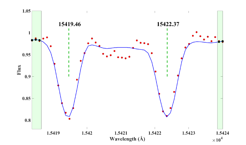
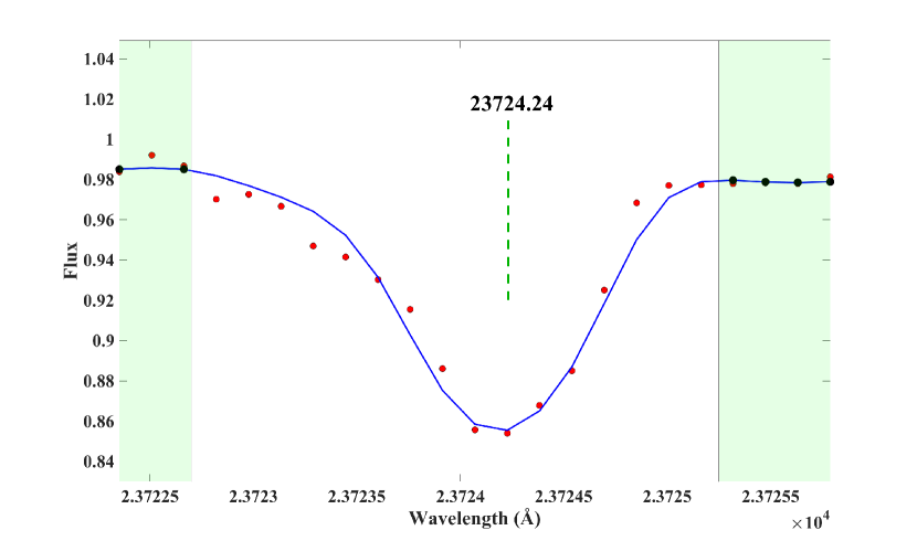
We identify the OH and CO lines that are nearly isolated from other species and have a well-defined shape (e.g., not distorted by noise or bad pixels, for example, due to artifacts or incomplete data reduction) and are also strong enough to be distinguished from the prevalent background H2O opacities common in M-dwarf spectra. In order to select the best lines for our study, the observed spectrum is first normalized relative to an initial guess of best-fit model over each line candidate. We generate a synthetic model (hereafter, Mod) associated with the star’s physical parameters (Section 3) and the solar absolute abundances for all elements333An estimate of the star’s best-fit model is associated with an absolute abundance equal to the solar absolute abundance plus metallicity [M/H], i.e., A(X)=A(X)☉+[M/H], for each element X, where A(X) is absolute abundance (Eq. 2). However, for this study, the metallicity of DH Tau A is assumed to be zero., which is an approximation of the star’s best-fit model. The most appropriate “normalizing” data points within the neighboring continuum/pseudocontinuum regions around each line candidate are specified through a linear fit to the residual, R=obs/syn, as a function of wavelength, where “obs” is the observed flux and “syn” is the synthetic flux, usually along with two iterative -clippings (2 and 1.5). This requires a trial-and-error inspection where different wavelength intervals in the continuum/pseudocontinuum around the line of interest are examined until at least one or two data points on each side of line are determined. On occasion, a couple of lines are close to one another, and the same normalizing regions around, and in some cases, also between these lines are chosen. The observed spectrum over each specific line is normalized after dividing the spectrum by the linear fit to the residuals at the determined normalizing data points. In Figures 1 and 2, we illustrate the selected normalizing regions and the corresponding normalizing data points for OH and CO lines, respectively. The blue line shows the synthetic model Mod and the red dots show the observed data normalized to this model using the normalizing points. The pseudocontinuum around spectral lines is dominated by prevailing, weak H2O lines, many of which are not well modeled due to incomplete H2O line lists. This generally results in a discrepancy between the observed and model spectrum within some pseudocontinuum regions (while these weak H2O lines have a negligible effect on the prominent analyzed lines), which makes it challenging to find appropriate data points for normalization. For many of the analyzed lines, we have therefore been able to determine only a few normalizing data points on each side within narrow intervals in the pseudocontinuum, though are sufficient for the normalization process. We select the OH and CO lines that show a reasonable consistency between the normalized observed spectrum and the synthetic model Mod. We exclude any line for which there is a significant discrepancy in depth and/or shape between the normalized observed spectrum and the estimated best-fit model. Our selected lines, including 24 OH and 8 CO lines are listed in Table 2. The oscillator strengths of these lines are also shown in the fourth column of this table.
The above-determined normalizing continuum/pseudocontinuum regions corresponding to each selected line are recorded and will then be used as input in the next step. In addition, for each analyzed line, we manually select a fitting or window, mostly far from the outermost part of the wings as another input to perform the minimization process, which is shown in the third column of Table 2. There are a variety of sources that may give rise to noise in stellar spectra such as photon noise or random fluctuations of the star light, stellar variability, sky background, the Earth’s atmospheric turbulence, and instrumental noise from telescope and detector. We find some spectral regions with relatively lower SNR values compared to other wavelength intervals, which are notably perturbed by noise, resulting in a substantial mismatch between the observed and model spectrum. Nevertheless, even within these regions, there is still a good agreement between the observed spectrum and synthetic model inside most of these strong absorption lines around their cores. Our choice of fitting windows also considers the minor effect of the dominant, weak H2O lines on the inner region of the prominent analyzed lines. Together with the previously inferred atmospheric parameters of the star (Section 3), we run AutoSpecFit to measure the abundances of oxygen and carbon. We show our results in Table 3; the number of analyzed lines, N, is shown in the second column, and the abundance [X/H] is presented in the third column, which is defined by
| (1) |
where denotes the number density of element X, indicates the number density of hydrogen, and A(X) shows the absolute abundance, i.e.,
| (2) |
These results show slightly supersolar carbon and oxygen abundances for DH Tau A.
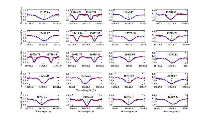
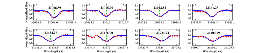
Figures 3 and 4 show the comparison between the resulting best-fit synthetic model and the target’s observed spectrum (normalized to the best-fit model) over all selected OH and CO lines, respectively. The best-fit model is associated with the star’s physical parameters and the O and C abundances inferred from this analysis. The O and C abundances are the weighted average abundances of all the analyzed OH and CO lines, respectively (see Hejazi et al. 2023, 2024 for more details), and the best-fit model does not necessarily show a perfect match to all these lines. Nevertheless, there is an excellent consistency between the observed spectrum and the determined best-fit model for most of the lines as seen in these figures by eye and confirmed by AutoSpecFit’s minimization process.
4.2 Abundance errors
To obtain the uncertainties of the inferred abundances, we first determine the random (statistical) errors using the standard error of the mean, i.e., =std/, where std is the standard deviation of the abundances from different lines of each species, as shown in the 9th column of Table 4. We also derive the systematic errors by determining the sensitivity of abundances to physical parameters. We deviate each parameter by its uncertainty (Section 3) in both positive and negative direction one at a time (Tables 3 and 4). We then carry out AutoSpecFit ten times, in each of which only one parameter is deviated in a specific direction while the other parameters are kept the same as the target’s parameters, and the abundances of carbon and oxygen are inferred from each run. The columns 4-12 of Table 3 and the columns 2-7 of Table 4 show the abundance (or absolute abundance)444Based on Eq. 1, since the Solar absolute abundance, A(X)☉, is constant, . variations due to the deviated parameters in both positive and negative directions relative to the inferred C and O abundances (i.e., [X/H], the third column of Table 3) as well as the average of absolute values of these variations () related to each parameter.
The above variations, in general, depend on the specific deviated parameter and the direction of deviation, i.e., positive or negative, as well as the particular element, i.e., carbon or oxygen. For example, the oxygen abundance is more sensitive to [M/H], as compared to the carbon abundance. On the other hand, the carbon abundance is more sensitive to , log(), and V, as compared to the oxygen abundance. The abundances of the two elements show roughly similar sensitivity to the veiling factor R with small differences depending on the direction in which this parameter is deviated. The systematic abundance error, , of each element is determined by the quadrature sum of the values from all parameters (the column 8 of Table 4):
| (3) |
where the index S takes the sequence T, M, G, V, and R corresponding to the deviated parameters , [M/H], log(), V, and R, respectively (Tables 3 and 4). The total abundance error, , is obtained by the quadrature sum of the random and systematic errors:
| (4) |
as shown in the last column of Table 4 for each element.
4.3 Carbon-to-Oxygen Abundance Ratio
We determine the star’s C/O abundance ratio using the equation:
| (5) |
where and indicate the number densities and A(C) and A(O) indicate the absolute abundances of elements C and O, respectively. We find a nearly solar C/O=0.555 for DH Tau A. For reference, the solar ratio is (C/O)☉=0.540 based on the solar abundances from Grevesse et al. (2007) (which we also use for our abundance analysis, see Hejazi et al. 2023, 2024 for additional information).
We employ the C and O abundance errors (Section 4.2) to calculate the uncertainty of the inferred C/O. Since the abundance ratio of the elements C and O depends on the subtraction of their absolute abundances (Eq. 5), their (correlated) systematic uncertainties related to the variation of each parameter largely cancel, making the contribution of all parameters (after adding in quadrature) to the total systematic error of C/O (Eq. 9) relatively small. It should be noted that the increase of the parameter uncertainties (even by 100) would not significantly change the total error of C/O ratio. This is because the increase in the uncertainty of each parameter will change the abundances of C and O in the same direction (positive or negative) such that the change in the subtraction of A(C)-A(O) would remain small. In contrast, the (uncorrelated) random (statistical) errors of the two elements are added together in quadrature, though the overall contribution of the random error to the total uncertainty is also small. The systematic error of C/O ratio is calculated as follows. We first determine the difference in the values between the two elements C and O for each parameter:
| (6) |
where S indicates the same parameter sequence as described for Eq. 3. These values show how the variation of a given parameter would change the difference between the abundances (or absolute abundances) of carbon and oxygen. Following the derivative equation:
| (7) |
and using Eq. 5, we derive the variation of C/O ratio due to the variation of for each parameter S (Eq. 6), as the systematic errors:
| (8) |
The total systematic error is obtained by the quadrature sum of all systematic errors:
| (9) |
The random error is calculated in the same way:
| (10) |
but is the quadrature sum of the random errors of C and O abundances (the 9th column of Table 4). Similar to Eq. 4, we derive a total uncertainty of 0.063 for the C/O ratio of the host star DH Tau A.
| Species | Central wavelength (Å) | window (Å) | log() | Comments |
|---|---|---|---|---|
| CO | 23006.89 | 23005.80-23007.70 | 5.457 | Blended with one CO line: 23006.56, log()=4.994 |
| CO | 23015.00 | 23014.10-23015.85 | 5.474 | Blended with one CO line: 23014.87, log()=4.985 |
| CO | 23023.52 | 23022.75-23024.45 | 5.491 | Blended with one CO line: 23023.61, log()=4.976 |
| CO | 23341.23 | 23340.55-23342.00 | 5.065 | Blended with one CO line: 23341.14, log()=4.481 |
| CO | 23434.27 | 23433.45-23435.15 | 5.239 | |
| CO | 23476.00 | 23475.20-23476.85 | 5.322 | Blended with two CO lines: |
| 23475.40, log()=4.743 and 23476.80, log()=5.075 | ||||
| CO | 23724.24 | 23722.90-23725.20 | 6.037 | Blended with one CO line: 23723.77, log()=5.865 |
| CO | 24104.19 | 24103.45-24105.10 | 5.456 | Blended with two CO lines: |
| 24104.25, log()=4.590 and 24104.62, log()=4.690 | ||||
| OH | 15129.66 | 15129.15-15130.15 | 5.499 | |
| OH | 15145.77 | 15145.20-15146.25 | 5.447 | |
| OH | 15147.94 | 15147.55-15148.40 | 5.447 | |
| OH | 15266.17 | 15265.70-15266.65 | 5.429 | |
| OH | 15278.52 | 15278.10-15278.95 | 5.382 | |
| OH | 15409.17 | 15408.60-15409.70 | 5.365 | Blended with one OH line: 15409.09, log()=6.605 |
| OH | 15419.46 | 15418.85-15420.00 | 5.323 | |
| OH | 15422.37 | 15421.85-15422.90 | 5.323 | |
| OH | 15572.08 | 15571.60-15572.60 | 5.269 | |
| OH | 15719.70 | 15719.20-15720.20 | 5.254 | |
| OH | 15726.72 | 15726.20-15727.25 | 5.219 | |
| OH | 15730.44 | 15729.90-15731.00 | 5.219 | |
| OH | 16052.77 | 16052.30-16053.25 | 4.910 | |
| OH | 16055.46 | 16054.95-16056.00 | 4.910 | |
| OH | 16065.05 | 16064.50-16065.50 | 5.159 | |
| OH | 16190.13 | 16189.70-16190.65 | 4.893 | Blended with one OH line: 16190.26, log()=5.145 |
| OH | 16260.16 | 16259.65-16260.65 | 5.087 | |
| OH | 16352.22 | 16351.60-16352.80 | 4.835 | |
| OH | 16534.58 | 16534.00-16535.15 | 4.746 | |
| OH | 16538.59 | 16538.00-16539.20 | 4.746 | |
| OH | 16704.36 | 16703.80-16705.00 | 4.732 | Blended with two OH lines: |
| 16703.88, log()=5.383 and 16704.70, log()=5.383 | ||||
| OH | 16872.28 | 16871.35-16872.80 | 4.975 | Blended with one OH line: 16871.90, log()=4.999 |
| OH | 16895.18 | 16894.60-16895.80 | 4.685 | |
| OH | 16909.29 | 16908.70-16909.95 | 4.654 |
| Species | N | [X/H] | [M/H] | log() | |||||||
|---|---|---|---|---|---|---|---|---|---|---|---|
| 30 | +30 | 0.10 | +0.10 | 0.05 | +0.05 | ||||||
| (K) | (K) | (K) | (dex) | (dex) | (dex) | (dex) | (dex) | (dex) | |||
| C (CO) | 8 | +0.064 | +0.011 | 0.011 | 0.011 | 0.003 | +0.005 | 0.004 | 0.040 | +0.047 | 0.044 |
| O (OH) | 24 | +0.050 | +0.007 | 0.001 | 0.004 | 0.015 | +0.033 | 0.024 | 0.028 | +0.041 | 0.035 |
Note. — The units are associated with the respective deviated parameters shown in the first row.
| Species | R | ||||||||
|---|---|---|---|---|---|---|---|---|---|
| 0.1 | +0.1 | 0.03 | +0.03 | ||||||
| km s-1 | km s-1 | km s-1 | |||||||
| C (CO) | 0.056 | +0.008 | 0.032 | 0.037 | +0.036 | 0.037 | 0.067 | 0.041 | 0.079 |
| O (OH) | 0.040 | +0.010 | 0.025 | 0.030 | +0.040 | 0.035 | 0.061 | 0.012 | 0.062 |
Note. — The units are associated with the respective deviated parameters shown in the first row.
5 Discussion: Host-Companion Connection
Our measurement of for DH Tau A is fully consistent with the value for the companion DH TAu b, (Xuan et al., 2024). This directly validates the chemical homogeneity in this system, which was already suggested in Xuan et al. (2024) based on previous measurements of Fe abundances for other stars in the Taurus star-forming region (Santos et al., 2008; D’Orazi et al., 2011). Our results indicate that the companion is compatible with forming via direct gravitational collapse, either from a disk or a molecular cloud. While formation via core accretion beyond the CO ice line also results in stellar C/O and metallicity as long as the companion accreted more solids than gas (Chachan et al., 2023; Xuan et al., 2024), this scenario is unlikely for DH Tau b due to various reasons. First, core accretion is expected to take several Myr to complete, but the DH Tau system is extremely young with an estimated age of Myr from isochrone fitting (Xuan et al., 2024). Second, the mass ratio between DH Tau b and DH Tau A is , which implies that a massive disk is required to form the companion. Massive disks with large host-to-companion mass ratios are prone to gravitational instability, which again makes the core accretion formation scenario unlikely.
We note that Xuan et al. (2024) also detected 13CO in DH Tau b, and found . In addition to the abundance ratio C/O, future studies should attempt to measure for the host stars of giant exoplanets (e.g. Coria et al., 2024; Xuan et al., 2024), which will allow a direct comparison with the abundance profiles of their companions. However, the fast rotation and veiling of these young host stars may obscure minor isotopologue signatures from carbon- and oxygen-bearing molecules (e.g. HO, 18OH, 13CO, C18O).
Nevertheless, there are other elemental abundance ratios in addition to C/O that may act as indicators of core accretion formation in sub-stellar companions. Certain volatile abundance ratios in the atmospheres of these sub-stellar objects, when comparable to their host star values, would be indicative of their formation via gravitational instability. When C/N, N/O, S/N, C/S, or O/S ratios deviate significantly from that of their host star, this is a counter-indication of formation via core accretion and subsequent gas/pebble accretion as the planet migrates throughout the disk (Turrini et al., 2021; Pacetti et al., 2022; Crossfield, 2023). With recent detections of H2O, CO, CO2, SO2, H2S, CH4, and NH3 in brown dwarfs and gas giant exoplanets (Schlawin et al., 2024; Hsu et al., 2024; Fu et al., 2024; Rafi et al., 2024; Yang et al., 2024; Powell et al., 2024; Nasedkin et al., 2024; Barrado et al., 2023), these volatile abundance ratios may be used for direct comparisons when measured in both the host star and in the sub-stellar companion and provide a better insight into their formation scenarios.
6 Summary
We measure the O and C abundances as well as the C/O abundance ratio of the young M-type star DH Tau A using its high-resolution IGRINS spectra ( 45000) in both the and band. We determine the star’s physical parameters (Table 1), which are then used as input for our abundance measurements. By a careful visual inspection, we select 24 OH (in the band) and 8 CO (in the band) lines (Table 2) to infer the elemental abundances of O and H, respectively. We briefly describe our approach to normalize the observed spectrum by illustrating two examples (Figures 1 and 2). We finally apply our automatic code, AutoSpecFit, which performs an iterative, line-by-line minimization over all the selected lines until the final abundances of O and C are reached simultaneously (Table 3).
We find a near-solar for the host star, which is completely consistent with that of the companion DH Tau b, . This confirms that the two components are chemically homogeneous, which suggests direct gravitational collapse (with a timescale of 1 Myr) as a more probable mechanism for the formation of the companion. Given the very young age of the system ( Myr), it is unlikely that the companion was formed through a core accretion process (with a typical time scale of several Myr).
The comparison between the chemical abundances of planets and substellar objects with those of their host stars can provide essential clues on the formation pathways of host-companion systems. With the advent of space-based telescopes such as JWST, chemical composition measurements for substellar companions have become possible. While the chemical abundances of many hotter JWST FGK-dwarf hosts have already been measured (e.g. Kolecki & Wang, 2022; Polanski et al., 2022), due to the complexity of M-dwarf spectra, only a small number of cooler JWST M-dwarf hosts have reported abundances (e.g. Hejazi et al., 2024; Melo et al., 2024). Spectroscopic analyses of M-type host stars, such as the one presented in this paper, are paramount to understanding the condition of protoplanetary disks and the subsequent formation of planets or low-mass substellar companions. This work has demonstrated successful near-infrared spectral fitting of an actively accreting M-dwarf star and will allow for the derivation of high-precision, multi-element abundances of several high-priority JWST M-dwarf exoplanet hosts and hosts to young, directly imaged exoplanets and brown dwarfs including the targets in Xuan et al. (2024) and many others.
Acknowledgements: We wish to thank the anonymous referee for their insightful comments and suggestions, which improved our manuscript. We express our appreciation to Justin Cantrell for his technical support with the high-performance computing system of the physics and astronomy department, Georgia State University, which was used for this study. N.H. and I.J.M.C. acknowledge support from NSF AAG grant No. 2108686 and from NASA ICAR grant No. NNH19ZDA001N. J.X. is supported by the NASA Future Investigators in NASA Earth and Space Science and Technology (FINESST) award #80NSSC23K1434.
This work used The Immersion Grating Infrared Spectrometer (IGRINS) was developed under a collaboration between the University of Texas at Austin and the Korea Astronomy and Space Science Institute (KASI) with the financial support of the US National Science Foundation under grants AST-1229522, AST-1702267 and AST-1908892, McDonald Observatory of the University of Texas at Austin, the Korean GMT Project of KASI, the Mt. Cuba Astronomical Foundation and Gemini Observatory. This paper includes data taken at The McDonald Observatory of The University of Texas at Austin.
References
- Abdurro’uf et al. (2022) Abdurro’uf, Accetta, Katherineand Aerts, C., Silva Aguirre, V., et al. 2022, ApJS, 259, 35, doi:10.3847/1538-4365/ac4414
- Alibert (2017) Alibert, Y. 2017, A&A, 606, A69, doi:10.1051/0004-6361/201630051
- Alibert et al. (2013) Alibert, Y., Carron, F., Fortier, A., et al. 2013, A&A, 558, A109, doi:10.1051/0004-6361/201321690
- Alvarez & Plez (1998) Alvarez, R., & Plez, B. 1998, A&A, 330, 1109, doi:10.48550/arXiv.astro-ph/9710157
- Barrado et al. (2023) Barrado, D., Mollière, P., Patapis, P., et al. 2023, Nature, 624, 263, doi:10.1038/s41586-023-06813-y
- Basri & Batalha (1990) Basri, G., & Batalha, C. 1990, ApJ, 363, 654, doi:10.1086/169374
- Bate (2012) Bate, M. R. 2012, MNRAS, 419, 3115, doi:10.1111/j.1365-2966.2011.19955.x
- Bergin et al. (2024) Bergin, E. A., Booth, R. A., Colmenares, M. J., & Ilee, J. D. 2024, ApJ, 969, L21, doi:10.3847/2041-8213/ad5839
- Biazzo et al. (2017) Biazzo, K., Frasca, A., Alcalá, J. M., et al. 2017, A&A, 605, doi:10.1051/0004-6361/201730850
- Bonnefoy et al. (2014) Bonnefoy, M., Chauvin, G., Lagrange, A.-M., et al. 2014, A&A, 562, A127, doi:10.1051/0004-6361/201118270
- Calvet et al. (1984) Calvet, N., Basri, G., & Kuhi, L. V. 1984, ApJ, 277, 725, doi:10.1086/161744
- Chachan et al. (2023) Chachan, Y., Knutson, H. A., Lothringer, J., & Blake, G. A. 2023, ApJ, 943, 112, doi:10.3847/1538-4357/aca614
- Coria et al. (2024) Coria, D. R., Hejazi, N., J.M., C. I., & Rhem, M. 2024, arXiv, 952, doi:10.48550/arXiv.2409.02286
- Cristofari et al. (2022) Cristofari, P. I., Donati, J. F., Masseron, T., et al. 2022, MNRAS, 511, 1893, doi:10.1093/mnras/stab3679
- Cristofari et al. (2023) Cristofari, P. I., Donati, J. F., Folsom, C. P., et al. 2023, MNRAS, 522, 1342, doi:10.1093/mnras/stad865
- Crossfield (2023) Crossfield, I. J. M. 2023, ApJ, 952, L18, doi:10.3847/2041-8213/ace35f
- Cushing et al. (2004) Cushing, M. C., Vacca, W. D., & Rayner, J. T. 2004, PASP, 116, 362, doi:10.1086/382907
- D’Orazi et al. (2011) D’Orazi, V., Biazzo, K., & Randich, S. 2011, A&A, 526, doi:10.1051/0004-6361/201015616
- Duque-Arribas et al. (2023) Duque-Arribas, C., Montes, D., Tabernero, H. M., et al. 2023, ApJ, 944, 106, doi:10.3847/1538-4357/acacf6
- Fischer et al. (2011) Fischer, W., Edwards, S., Hillenbrand, L., & Kwan, J. 2011, ApJ, 730, 73, doi:10.1088/0004-637X/730/2/73
- Foreman-Mackey et al. (2013) Foreman-Mackey, D., Hogg, D. W., & Lang, Dustin a d Goodman, J. 2013, Publications of the Astronomical Society of the Pacific, 125, 925, doi:10.1086/670067
- Fortney (2012) Fortney, J. J. 2012, ApJ, 747, L27, doi:10.1088/2041-8205/747/2/L27
- Fu et al. (2024) Fu, G., Welbanks, L., Deming, D., et al. 2024, Nature, 632, 752, doi:10.1038/s41586-024-07760-y
- Gaia Collaboration et al. (2021) Gaia Collaboration, G., Brown, A. G. A., Vallenari, A., et al. 2021, A&A, 649, 20, doi:10.1051/0004-6361/202039657
- Gandhi et al. (2023) Gandhi, S., de Regt, S., Snellen, I., et al. 2023, ApJ, 957, L36, doi:10.3847/2041-8213/ad07e2
- Grevesse et al. (2007) Grevesse, N., Asplund, M., & Sauval, A. J. 2007, Space Sci. Rev., 130, 105, doi:10.1007/s11214-007-9173-7
- Gully-Santiago et al. (2012) Gully-Santiago, M., Wang, W., Deen, C., & Jaffe, D. 2012, in Society of Photo-Optical Instrumentation Engineers (SPIE) Conference Series, Vol. 8450, Modern Technologies in Space- and Ground-based Telescopes and Instrumentation II, ed. R. Navarro, C. R. Cunningham, & E. Prieto, 84502S, doi:10.1117/12.926434
- Gustafsson et al. (2008) Gustafsson, B., Edvardsson, B., Eriksson, K., et al. 2008, A&A, 486, 951, doi:10.1051/0004-6361:200809724
- Han et al. (2012) Han, J.-Y., Yuk, I.-S., Ko, K., et al. 2012, in Society of Photo-Optical Instrumentation Engineers (SPIE) Conference Series, Vol. 8550, Optical Systems Design 2012, ed. D. G. Smith, J.-L. M. Tissot, L. Mazuray, T. E. Kidger, F. Wyrowski, J. M. Raynor, R. Wartmann, S. David, A. Erdmann, A. P. Wood, P. Benítez, & M. C. de la Fuente, 85501B, doi:10.1117/12.981169
- Hawkins et al. (2020) Hawkins, K., Lucey, M., Ting, Y.-S., et al. 2020, MNRAS, 492, 1164, doi:10.1093/mnras/stz3132
- Hejazi et al. (2022) Hejazi, N., Lépine, S., & Nordlander, T. 2022, ApJ, 927, 122, doi:10.3847/1538-4357/ac4e16
- Hejazi et al. (2023) Hejazi, N., Crossfield, I. J. M., Nordlander, T., et al. 2023, The Astrophysical Journal, 949, 79, doi:10.3847/1538-4357/accb97
- Hejazi et al. (2024) Hejazi, N., Crossfield, I. J. M., Souto, D., et al. 2024, ApJ, 973, 31, doi:10.3847/1538-4357/ad61dc
- Hoch et al. (2023) Hoch, K. K. W., Konopacky, Q. M., Theissen, C. A., et al. 2023, AJ, 166, 85, doi:10.3847/1538-3881/ace442
- Holstein et al. (2021) Holstein, R. G. V., Stolker, T., Jensen-Clem, R., et al. 2021, Astronomy and Astrophysics, 647, doi:10.1051/0004-6361/202039290
- Hood et al. (2024) Hood, C. E., Mukherjee, S., Fortney, J. J., et al. 2024, arXiv e-prints, arXiv:2402.05345, doi:10.48550/arXiv.2402.05345
- Horne (1986) Horne, K. 1986, PASP, 98, 609, doi:10.1086/131801
- Hsu et al. (2024) Hsu, C.-C., Wang, J. J., Xuan, J. W., et al. 2024, ApJ, 971, 9, doi:10.3847/1538-4357/ad58d3
- Ilee et al. (2017) Ilee, J. D., Forgan, D. H., Evans, M. G., et al. 2017, MNRAS, 472, 189, doi:10.1093/mnras/stx1966
- Itoh et al. (2005) Itoh, Y., Hayashi, M., Tamura, M., et al. 2005, ApJ, 620, 984, doi:arXiv:astro-ph/0411177
- Jeong et al. (2014) Jeong, U., Chun, M.-Y., Oh, J. S., et al. 2014, in Society of Photo-Optical Instrumentation Engineers (SPIE) Conference Series, Vol. 9154, High Energy, Optical, and Infrared Detectors for Astronomy VI, ed. A. D. Holland & J. Beletic, 91541X, doi:10.1117/12.2055589
- Jönsson et al. (2020) Jönsson, H., Holtzman, J. A., Allende Prieto, C., et al. 2020, AJ, 160, 120, doi:10.3847/1538-3881/aba592
- Joy (1949) Joy, A. H. 1949, ApJ, 110, 424, doi:10.1086/145217
- Kaplan et al. (2024) Kaplan, K., Lee, J.-J., Sawczynec, E., & Kim, H.-J. 2024, igrins/plp, 3.0.0, Zenodo, doi:10.5281/zenodo.11080095
- Kenyon & Hartmann (1987) Kenyon, S. J., & Hartmann, L. 1987, ApJ, 323, 714, doi:10.1086/165866
- Kolecki & Wang (2022) Kolecki, J. R., & Wang, J. 2022, AJ, 164, 87, doi:10.3847/1538-3881/ac7de3
- Kratter & Lodato (2016) Kratter, K., & Lodato, G. 2016, Annual Review of Astronomy and Astrophysics, 54, 271, doi:10.1146/annurev-astro-081915-023307
- Kraus & Hillenbrand (2009) Kraus, A. L., & Hillenbrand, L. A. 2009, ApJ, 703, 1511, doi:10.1088/0004-637X/703/2/1511
- Kurucz (1979) Kurucz, R. L. 1979, ApJS, 40, 1, doi:10.1086/190589
- Landman et al. (2024) Landman, R., Stolker, T., Snellen, I. A. G., et al. 2024, A&A, 682, A48, doi:10.1051/0004-6361/202347846
- López-Valdivia et al. (2021) López-Valdivia, R., Sokal, K. R., Mace, G. N., et al. 2021, ApJ, 921, 53, doi:10.3847/1538-4357/ac1a7b
- Mace et al. (2016) Mace, G., Kim, H., Jaffe, D. T., et al. 2016, in Society of Photo-Optical Instrumentation Engineers (SPIE) Conference Series, Vol. 9908, Ground-based and Airborne Instrumentation for Astronomy VI, ed. C. J. Evans, L. Simard, & H. Takami, 99080C, doi:10.1117/12.2232780
- Mann et al. (2015) Mann, A. W., Feiden, G. A., Gaidos, E., Boyajian, T., & von Braun, K. 2015, ApJ, 804, 64, doi:10.1088/0004-637X/804/1/64
- Mann et al. (2019) Mann, A. W., Dupuy, T., Kraus, A. L., et al. 2019, ApJ, 871, 63, doi:10.3847/1538-4357/aaf3bc
- Martinez & Kraus (2021) Martinez, R. A., & Kraus, A. L. 2021, The Astronomical Journal, 163, 36, doi:10.3847/1538-3881/ac3745
- Melo et al. (2024) Melo, E., Souto, D., Cunha, K., et al. 2024, doi:10.48550/arXiv.2406.00111
- Miles et al. (2023) Miles, B. E., Biller, B. A., Patapis, P., et al. 2023, ApJ, 946, L6, doi:10.3847/2041-8213/acb04a
- Mollière et al. (2020) Mollière, P., Stolker, T., Lacour, S., et al. 2020, Astronomy and Astrophysics, 640, A131, doi:10.1051/0004-6361/202038325
- Moon et al. (2012) Moon, B., Wang, W., Park, C., et al. 2012, in Society of Photo-Optical Instrumentation Engineers (SPIE) Conference Series, Vol. 8450, Modern Technologies in Space- and Ground-based Telescopes and Instrumentation II, ed. R. Navarro, C. R. Cunningham, & E. Prieto, 845048, doi:10.1117/12.925702
- Nasedkin et al. (2024) Nasedkin, E., Mollière, P., Lacour, S., et al. 2024, A&A, 687, A298, doi:10.1051/0004-6361/202449328
- Natta et al. (2001) Natta, A., Prusti, T., Neri, R., et al. 2001, A&A, 371, 186, doi:10.1051/0004-6361:20010334
- Offner et al. (2010) Offner, S. S. R., Kratter, K. M., Matzner, C. D., Krumholz, M. R., & Klein, R. I. 2010, ApJ, 725, 1485, doi:10.1088/0004-637X/725/2/1485
- Oh et al. (2014) Oh, J. S., Park, C., Cha, S.-M., et al. 2014, in Society of Photo-Optical Instrumentation Engineers (SPIE) Conference Series, Vol. 9147, Ground-based and Airborne Instrumentation for Astronomy V, ed. S. K. Ramsay, I. S. McLean, & H. Takami, 914739, doi:10.1117/12.2055651
- Ohno & Fortney (2023) Ohno, K., & Fortney, J. J. 2023, The Astrophysical Journal, 946, 18, doi:10.3847/1538-4357/acafed
- Pacetti et al. (2022) Pacetti, E., Turrini, D., Schisano, E., et al. 2022, ApJ, 937, 36, doi:10.3847/1538-4357/ac8b11
- Park et al. (2014) Park, C., Jaffe, D. T., Yuk, I.-S., et al. 2014, in Society of Photo-Optical Instrumentation Engineers (SPIE) Conference Series, Vol. 9147, Ground-based and Airborne Instrumentation for Astronomy V, ed. S. K. Ramsay, I. S. McLean, & H. Takami, 91471D, doi:10.1117/12.2056431
- Patience et al. (2012) Patience, J., King, R. R., De Rosa, R. J., et al. 2012, A&A, 540, A85, doi:10.1051/0004-6361/201118058
- Plez (2012) Plez, B. 2012, Turbospectrum: Code for spectral synthesis, Astrophysics Source Code Library, record ascl:1205.004
- Polanski et al. (2022) Polanski, A. S., Crossfield, I. J. M., Howard, A. W., Isaacson, H., & Rice, M. 2022, Research Notes of the AAS, 6, 155, doi:10.3847/2515-5172/ac8676
- Pollack et al. (1996) Pollack, J. B., Hubickyj, O., Bodenheimer, P., et al. 1996, Icarus, 124, 62, doi:10.1006/icar.1996.0190
- Powell et al. (2024) Powell, D., Feinstein, A. D., Lee, E. K. H., et al. 2024, Nature, 626, 979, doi:10.1038/s41586-024-07040-9
- Rafi et al. (2024) Rafi, S. A., Nugroho, S. K., Tamura, M., Nortmann, L., & Sánchez-López, A. 2024, AJ, 168, 106, doi:10.3847/1538-3881/ad5be9
- Reiners & Basri (2007) Reiners, A., & Basri, G. 2007, ApJ, 656, 1121, doi:10.1086/510304
- Roccatagliata et al. (2020) Roccatagliata, V., Franciosini, E., Sacco, G. G., Randich, S., & Sicilia-Aguilar, A. 2020, A&A, 638, A85, doi:10.1051/0004-6361/201936401
- Santos et al. (2008) Santos, N. C., Melo, C., James, D. J., et al. 2008, A&A, 480, 889, doi:10.1051/0004-6361:20079083
- Sawczynec et al. (2023) Sawczynec, E., Mace, G., Gully-Santiago, M., & Jaffe, D. 2023, in American Astronomical Society Meeting Abstracts, Vol. 241, American Astronomical Society Meeting Abstracts, 207.14
- Schlawin et al. (2024) Schlawin, E., Mukherjee, S., Ohno, K., et al. 2024, AJ, 168, 104, doi:10.3847/1538-3881/ad58e0
- Souto et al. (2017) Souto, D., Cunha, K., García-Hernández, D. A., et al. 2017, ApJ, 835, 239, doi:10.3847/1538-4357/835/2/239
- Souto et al. (2018) Souto, D., Unterborn, C. T., Smith, V. V., et al. 2018, ApJ, 860, L15, doi:10.3847/2041-8213/aac896
- Souto et al. (2022) Souto, D., Cunha, K., Smith, V. V., et al. 2022, ApJ, 927, 123, doi:10.3847/1538-4357/ac4891
- Sprague et al. (2022) Sprague, D., Culhane, C., Kounkel, M., et al. 2022, AJ, 163, 152, doi:10.3847/1538-3881/ac4de7
- Stempels & Piskunov (2003) Stempels, H. C., & Piskunov, N. 2003, A&A, 408, 693, doi:10.1051/0004-6361:20030637
- Turrini et al. (2021) Turrini, D., Schisano, E., Fonte, S., et al. 2021, The Astrophysical Journal, 909, 40, doi:10.3847/1538-4357/abd6e5
- van Holstein et al. (2021) van Holstein, R. G., Stolker, T., Jensen-Clem, R., et al. 2021, A&A, 647, A21, doi:10.1051/0004-6361/202039290
- Wang et al. (2023a) Wang, J., Wang, J. J., Ruffio, J.-B., et al. 2023a, The Astronomical Journal, 165, 4, doi:10.3847/1538-3881/ac9f19
- Wang et al. (2023b) Wang, R., Luo, A. L., Zhang, S., et al. 2023b, ApJS, 266, 40, doi:10.3847/1538-4365/acce36
- Wang et al. (2010) Wang, W., Gully-Santiago, M., Deen, C., Mar, D. J., & Jaffe, D. T. 2010, in Society of Photo-Optical Instrumentation Engineers (SPIE) Conference Series, Vol. 7739, Modern Technologies in Space- and Ground-based Telescopes and Instrumentation, ed. E. Atad-Ettedgui & D. Lemke, 77394L, doi:10.1117/12.857164
- Wang et al. (2024) Wang, Y., Zhang, L., Su, T., Han, X. L., & Misra, P. 2024, A&A, 686, A164, doi:10.1051/0004-6361/202348342
- Xuan et al. (2022) Xuan, J. W., Wang, J., Ruffio, J.-B., et al. 2022, The Astrophysical Journal, 937, 54, doi:10.3847/1538-4357/ac8673
- Xuan et al. (2024) Xuan, J. W., Hsu, C.-C., Finnerty, L., et al. 2024, ApJ, 970, 71, doi:10.3847/1538-4357/ad4796
- Xuan et al. (2024) Xuan, J. W., Wang, J., Finnerty, L., et al. 2024, The Astrophysical Journal, 962, 10, doi:10.3847/1538-4357/ad1243
- Yang et al. (2024) Yang, J., Hammond, M., Piette, A. A. A., et al. 2024, MNRAS, 532, 460, doi:10.1093/mnras/stae1427
- Yu et al. (2023) Yu, J., Khanna, S., Themessl, N., et al. 2023, ApJS, 264, 41, doi:10.3847/1538-4365/acabc8
- Yuk et al. (2010) Yuk, I.-S., Jaffe, D. T., Barnes, S., et al. 2010, in Society of Photo-Optical Instrumentation Engineers (SPIE) Conference Series, Vol. 7735, Ground-based and Airborne Instrumentation for Astronomy III, ed. I. S. McLean, S. K. Ramsay, & H. Takami, 77351M, doi:10.1117/12.856864
- Zhang et al. (2021a) Zhang, Y., Snellen, I. A. G., & Mollière, P. 2021a, A&A, 656, A76, doi:10.1051/0004-6361/202141502
- Zhang et al. (2021b) Zhang, Y., Snellen, I. A. G., Bohn, A. J., et al. 2021b, Nature, 595, 370, doi:10.1038/s41586-021-03616-x
- Zhang et al. (2024) Zhang, Y., Xuan, J. W., Mawet, D., et al. 2024, arXiv e-prints, arXiv:2407.20952, doi:10.48550/arXiv.2407.20952
- Zhang et al. (2023) Zhang, Z., Mollière, P., Hawkins, K., et al. 2023, AJ, 166, 198, doi:10.3847/1538-3881/acf768
- Zhou et al. (2014) Zhou, Y., Herczeg, G. J., Kraus, A. L., Metchev, S., & Cruz, K. L. 2014, ApJ, 783, L17, doi:10.1088/2041-8205/783/1/L17
- Öberg et al. (2011) Öberg, K. I., Murray-Clay, R., & Bergin, E. A. 2011, ApJ, 743, L16, doi:10.1088/2041-8205/743/1/L16