Decay of amplitude of a harmonic oscillator with weak nonlinear damping

Abstract

We demonstrate how to derive approximate expressions for the amplitude decay of a weakly damped harmonic oscillator in case of a damping force with constant magnitude (sliding friction) and in case of a damping force quadratic in velocity (air resistance), without solving the associated equations of motion. This is achieved using a basic understanding of the undamped harmonic oscillator and the connection between the damping force’s power and the energy dissipation rate. Our approach is based on adapting the trick of adding the energy dissipation rates corresponding to two specific pairs of initial conditions, which was recently used to derive the exponential decay of the amplitude in case of viscous damping, to these two types of damping. We obtain two first-order differential equations from which we get the time-dependent amplitudes corresponding to both damping forces. By comparing our approximate solutions with the exact solutions in the case of sliding friction and with the approximate solutions given by a another well-known method in the case of air resistance, we find that our solutions describe well the dynamics of the oscillator in the regime of weak damping with these two forces. The physical concepts and mathematical techniques we employ are well-known to first-year undergraduates.

I Introduction

The damped harmonic oscillator with damping force linear in velocity, i.e. with viscous damping, is regularly covered in physics textbooks for the first year of undergraduate studies, e.g., see Cutnell8 ; Resnick10 ; Young2020university . In these same books, motions under the influence of sliding friction Cutnell8 ; Resnick10 ; Young2020university and air resistance (drag force) Resnick10 ; Young2020university are also covered, but only in the context of unidirectional motions such as, e.g., sliding down an inclined plane and a free fall in the air, while the analysis of the influence of these forces on the dynamics of the harmonic oscillator is omitted. Furthermore, even in physics textbooks that give a more thorough analysis of vibrations at a more advanced undergraduate level, the influence of sliding friction and air resistance on the dynamics of oscillating systems is not considered, e.g., see Waves . The reason for this is that sliding friction, i.e. damping of constant magnitude, and air resistance, i.e. damping quadratic in velocity, require a mathematical treatment that is demanding for first-year undergraduates, while on the other hand, the dynamics of a viscously damped harmonic oscillator can be analyzed in a fashion known to students at that level. The main pedagogical advantage in the case of viscous damping is that the solution of the corresponding equation of motion can be written analytically in a closed form valid for all times, and such a solution is easy to analyze. But even in that case, textbooks Cutnell8 ; Resnick10 ; Young2020university ; Waves avoid the formal derivation of the solution, and usually just state the solution without derivation.

In case of harmonic oscillator damped with sliding friction (often called Coulomb damping, e.g. see Coulomb ) the corresponding equation of motion can be solved exactly by splitting the motion into left and right moving segments Lapidus ; AviAJP ; Grk2 , i.e. it can be solved in a straightforward albeit cumbersome manner, since the motion needs to be analyzed over half-cycles. Furthermore, the solution thus obtained cannot be put into a closed form that is valid for all times Lapidus ; Grk2 ; Kamela . In the case of a harmonic oscillator damped with air resistance, the treatment is even more demanding, since the corresponding equation of motion is a nonlinear differential equation that cannot be solved analytically and approximate or numerical methods must be used Smith ; Mungan ; Wang ; Grk2 .

All three types of damping were investigated in the regime of weak damping, both experimentally and theoretically, in Wang . On the theoretical side, amplitude decay for all three types of damping has been derived using the approximation that the amplitude remains constant over time intervals of one period in length and using the energy dissipation rate averaged over these time intervals, and the validity of the approximate solutions thus obtained was confirmed by experiments Wang . In case of viscous damping, approach used in Wang gives exponential amplitude decay, and purely exponential approximation of the energy decay. In a recent paper LelasPezer viscous damping was considered and the exponential amplitude decay of a weakly damped harmonic oscillator was derived, using only basic knowledge about the undamped harmonic oscillator and the connection between the power of the damping force and the energy dissipation rate. The trick is in adding the dissipation rates corresponding to two specific pairs of initial conditions LelasPezer . In this approach there is no need for time averaging over a period which is used in Wang . There are two variants of the approach used in LelasPezer , i.e. the authors focus on the variant that gives the exponential amplitude decay and an excellent approximation of full behaviour of the energy decay, and briefly comment on a somewhat simpler version of the same approach that also gives an exponential amplitude decay, but only an exponential approximation of the energy decay. It was pointed out that the trick of adding energy dissipation rates does not work in the case of sliding friction and air resistance, i.e. it does not lead to a simple first order differential equation for the amplitude, as in the case of viscous damping LelasPezer .

The aim of this paper is to adapt the reasoning and the trick introduced in LelasPezer to study harmonic oscillators weakly damped by sliding friction or air resistance. This paper is organized into six sections. In section II, we present the theory and approximations needed in our approach, comment on the case of viscous damping and state the problem we are dealing with. In section III, we derive the linear amplitude decay in case of sliding friction. In section IV, we derive the amplitude decay in case of air resistance. In section V, we compare our results in case of sliding friction with the results obtained by method introduced in Wang and exact results Grk2 . In section VI, we compare our results in case of air resistance with the results obtained by method introduced in Wang . In section VII, we comment on some issues with the choices of initial conditions in our derivations, and summarize important findings of the paper.

II Basic theory, approximations we use, damping linear in velocity, and posing of the problems that we address

As an example of a damped harmonic oscillator, we consider a block of mass $m$ that oscillates under the influence of the restoring force of an ideal spring of stiffness $k$ and the damping force $F_{d}(t)$. The equation of motion of this system is

$$ma(t)=F_{d}(t)-kx(t)\,,$$ (1)

where $x(t)$ is the block’s displacement from the equilibrium position, and $a(t)=d^{2}x(t)/dt^{2}$ is its acceleration. We consider three types of damping in this paper. Viscous damping, described with the force

$$F_{d}(t)=-b\,v(t)\,,$$ (2)

where $b>0$ is the damping constant and $v(t)=dx(t)/dt$ is the velocity of the block Young2020university ; Resnick10 . Sliding friction

$$F_{d}(t)=-\text{sgn}[v(t)]\,\mu mg\,,$$ (3)

where $\mu>0$ is the coefficient of sliding friction Young2020university ; Resnick10 , and we use the sign function

$$\text{sgn}\left[v(t)\right]=\begin{cases}\begin{tabular}[]{@{}cl@{}}$1$&if\, $v(t)$ $>$ $0$\\ $0$&if\, $v(t)$ $=$ $0$\\ $-1$&if\, $v(t)$ $<$ $0$\end{tabular}\end{cases}$$ (4)

to take into account that damping force always has a direction opposite to the direction of the velocity. The third case is the air resistance, described with the force of the form

$$F_{d}(t)=-\text{sgn}[v(t)]\,Cv^{2}(t)\,,$$ (5)

where $C>0$ is a constant Young2020university ; Resnick10 . In the context of air resistance, we can imagine that we have a sphere of mass $m$ attached to a spring, rather than the block, since usually air resistance of spherical objects is considered in the physics textbooks Young2020university ; Resnick10 , and in that case $C=c\rho A/2$, where $c$ is experimentally determined drag coefficient, $\rho$ is the air density, and $A$ is the cross sectional area of the sphere Resnick10 .

The energy (potential plus kinetic) of the block-spring system is given by

$$E(t)=\frac{kx^{2}(t)}{2}+\frac{mv^{2}(t)}{2}\,.$$ (6)

If we put $F_{d}(t)=0$ in (1) we get the equation of the undamped harmonic oscillator Resnick10 , with general solution $x(t)=A_{0}\cos(\omega_{0}t+\phi_{0})$, where $\omega_{0}=\sqrt{k/m}$ is the angular frequency of the undamped system, while $A_{0}$ and $\phi_{0}$ are constants (amplitude and initial phase) that are determined from a pair of initial conditions $\left(x(0)=x_{0},v(0)=v_{0}\right)$. The undamped system oscillates with conserved, i.e. constant, energy Resnick10 . For the damped systems, i.e. for $F_{d}(t)\neq 0$, the energy is not conserved due to the power of the damping force $P_{d}(t)=F_{d}(t)v(t)$, and the energy dissipation rate is given by Young2020university

$$\frac{dE(t)}{dt}=F_{d}(t)v(t)\,.$$ (7)

Equation (7) is valid for all three types of damping, i.e for (2), (3) and (5). Since the direction of the damping force is opposite to the direction of the velocity at all times, $F_{d}(t)v(t)\leq 0$ is valid $\forall t$. Thus, equation (7) tells us that the energy of the damped system decreases monotonically with time, i.e. $\frac{dE(t)}{dt}\leq 0$ for all $t\geq 0$, and $\frac{dE(t)}{dt}=0$ holds at the turning points, i.e. at instants when $v(t)=0$.

In a recent paper LelasPezer , damping linear in velocity, i.e. (2), was considered and the exponential amplitude decay and the full behaviour of the energy decay in the weak damping regime were derived using a simple trick of adding the energy dissipation rates (7) corresponding to two specific pairs of initial conditions. In addition, the authors briefly commented on a somewhat simpler version of the approach used, which also leads to an exponential decay of amplitude, but gives only a purely exponential decay of energy (see section V in LelasPezer ). Here we will recapitulate this simpler version of the approach introduced in LelasPezer , and we show how to adapt it for the other two types of damping in the following sections. Thus, in what follows we first consider $F_{d}(t)=-bv(t)$, with the power of the damping force $P_{d}(t)=-bv^{2}(t)$.

Two pairs of initial conditions, i.e. $(x_{1}(0)=x_{0},v_{1}(0)=0)$ and $(x_{2}(0)=0,v_{2}(0)=\omega_{0}x_{0})$, were considered in LelasPezer . The first pair has purely potential initial energy, and the second pair has purely kinetic initial energy, and, due to the chosen value of $v_{2}(0)$, both pairs have the same initial energy $E_{0}=m\omega_{0}^{2}x_{0}^{2}/2$. The solutions of equation (1) in the undamped case, corresponding to these initial conditions, are $x_{1}(t)=x_{0}\cos(\omega_{0}t)$ and $x_{2}(t)=x_{0}\sin(\omega_{0}t)$. It is argued in LelasPezer that it can be easily explained to students, based on analysis of graphical representations of experimental data or exact solutions, without giving them any insight into the analytical form of the exact solutions, that the defining characteristics of the weak damping regime are that the frequency and the initial phase remain approximately the same as in the undamped case, while the amplitude of the oscillations decreases very slowly over time, i.e. it decrease only slightly during one full oscillation (one period) of the system. Furthermore, it can be argued, also based only on analysis of graphical representations of experimental data or exact solutions, that the amplitude decreases in the same fashion for both pairs of considered initial conditions LelasPezer . Thus, in the case of weak damping linear in velocity we can take that the solutions of the equation (1), for the chosen initial conditions, are approximately of the form

$$x_{1}(t)=x_{0}f(t)\cos(\omega_{0}t)$$ (8)

and

$$x_{2}(t)=x_{0}f(t)\sin(\omega_{0}t)\,,$$ (9)

where $f(t)$ is the unknown function that describes the amplitude decrease in time. The corresponding velocities are

$$v_{1}(t)=\frac{dx_{1}(t)}{dt}=-\omega_{0}\left(x_{0}f(t)\sin(\omega_{0}t)+x_{0}\frac{\dot{f}(t)}{\omega_{0}}\cos(\omega_{0}t)\right)\,$$ (10)

and

$$v_{2}(t)=\frac{dx_{2}(t)}{dt}=\omega_{0}\left(x_{0}f(t)\cos(\omega_{0}t)+x_{0}\frac{\dot{f}(t)}{\omega_{0}}\sin(\omega_{0}t)\right)\,.$$ (11)

Since the amplitude changes very slowly in comparison to the oscillating part of (8) and (9), the rate of change of function $f(t)$ over time has to be much slower than the rate of change of $\cos(\omega_{0}t)$ and $\sin(\omega_{0}t)$, which is of the order $\omega_{0}$. We can conclude that $|\dot{f}(t)|\ll\omega_{0}$ holds for weak damping for all time, i.e., for $t\geq 0$ (we have put absolute value because we can expect the negative derivative of $f(t)$ since the amplitude decreases with time). Thus, due to $|\dot{f}(t)|/\omega_{0}\ll 1$, we can take that the velocities, corresponding to considered initial conditions, are approximately of the form

$$v_{1}(t)=-\omega_{0}x_{0}f(t)\sin(\omega_{0}t)\,$$ (12)

and

$$v_{2}(t)=\omega_{0}x_{0}f(t)\cos(\omega_{0}t)\,.$$ (13)

It is easy to see that $f(0)=1$ must hold, for the functions (8) and (13) to satisfy the initial conditions $x_{1}(0)=x_{0}$ and $v_{2}(0)=\omega_{0}x_{0}$. Since $f(0)=1$ holds, and the function monotonically decreases, we can easily conclude that $f(t)\geq 0$ must also hold, for all $t\geq 0$.

By using displacements (8) and (9), and velocities (12) and (13), in (6), we get the corresponding energies

$$E_{1}(t)=E_{2}(t)=\frac{m\omega_{0}^{2}x_{0}^{2}f^{2}(t)}{2}\,.$$ (14)

The first derivatives of energies $E_{1}(t)$ and $E_{2}(t)$ are

$$\frac{dE_{1}(t)}{dt}=\frac{dE_{2}(t)}{dt}=m\omega_{0}^{2}x_{0}^{2}f(t)\frac{df(t)}{dt}\,.$$ (15)

Using velocities (12) and (13) in $P_{d}(t)=-bv^{2}(t)$ we get approximate expressions for the power of the damping force, corresponding to each pair of considered initial conditions, i.e.

$$P_{d1}(t)=-b\omega_{0}^{2}x_{0}^{2}f^{2}(t)\sin^{2}(\omega_{0}t)\,$$ (16)

and

$$P_{d2}(t)=-b\omega_{0}^{2}x_{0}^{2}f^{2}(t)\cos^{2}(\omega_{0}t)\,.$$ (17)

By using (15) to approximate the left hand side of the energy dissipation rate (7), and relations (16) and (17) to approximate the right hand side of (7), i.e. by approximating the energy dissipation rate $dE(t)/dt=P_{d}(t)$ for both pairs of initial conditions, we get

$$\frac{df(t)}{dt}=-\frac{b}{m}f(t)\sin^{2}(\omega_{0}t)\,.$$ (18)

and

$$\frac{df(t)}{dt}=-\frac{b}{m}f(t)\cos^{2}(\omega_{0}t)\,.$$ (19)

We can easily see that by adding (18) and (19) we get

$$\frac{df(t)}{dt}=-\frac{b}{2m}f(t)\,,$$ (20)

where we used the simple trigonometric identity $\sin^{2}(\omega_{0}t)+\cos^{2}(\omega_{0}t)=1$. Using substitution $\alpha=-b/(2m)$, (20) becomes $df(t)/dt=\alpha f(t)$, and both first year undergraduates and high school students know that the function $f(t)=e^{\alpha t}$ satisfies this differential equation. Thus, we get the exponential decay of amplitude in case of weak damping linear in velocity, i.e. $f(t)=e^{-\frac{b}{2m}t}$, without formally solving differential equation (1) and without any prior insight in the analytical form of its solutions. Furthermore, it was shown in LelasPezer how to derive the weak damping condition

$$b\ll 2\sqrt{km}$$ (21)

once we found $f(t)$.

Now we return to the analysis of the other two types of damping. All three types of damping have been experimentally investigated in the weak damping regime, e.g., see Wang . By considering the figures with the results of these experiments, even without any prior knowledge of damped systems with the other two types of damping, students can easily conclude that the defining characteristics of a weak damping regime in the other two cases are qualitatively the same as for the damping linear in velocity, i.e. the frequency and the initial phase remain approximately the same as in the undamped case, while the amplitude of the oscillations decreases very slowly over time. Thus, the approximate form of the solutions of equation (1), i.e. (8) and (9), and the corresponding velocities, i.e. (12) and (13), can be taken in case of weak damping with (3) and (5) as well. Of course, the function $f(t)$ is expected to be specific for each type of damping, since each type of damping has the corresponding power of the damping force different than the other two.

It is noted in LelasPezer that the trick of adding the dissipation rates does not work for the other two types of damping. The reason for this is that the power of the damping force is not proportional to the square of the velocity for the other two types of damping, i.e. if the same approach is applied directly to the other two types of damping, one does not obtain expressions that can be simplified using simple trigonometric identities. In this paper, we deal with the following problems. How to adapt the approach used in LelasPezer to obtain the amplitude decay, i.e. the function $f(t)$, in case of weak damping with damping forces (3) and (5)? What conditions must $\mu$ and $C$ satisfy, in relation to other parameters of the system, for the dynamics of the harmonic oscillator to be weakly damped?

III Amplitude decay in case of weak sliding friction

As we commented in the previous section, in case of weak damping with $F_{d}(t)=-\text{sgn}(v(t))\mu mg$ we can also take (8) and (9) for the approximate form of the solutions of equation (1), and (12) and (13) as the corresponding approximate velocities. Thus, the approximate energies $E_{1}(t)$ and $E_{2}(t)$, corresponding to considered pairs of initial conditions, and their first derivatives are again given by relations (14) and (15). The difference is in the expressions for the the power of the damping force, which are now

$$P_{d1}(t)=-\text{sgn}[v_{1}(t)]\mu mg\,v_{1}(t)\,$$ (22)

and

$$P_{d2}(t)=-\text{sgn}[v_{2}(t)]\mu mg\,v_{2}(t)\,.$$ (23)

It is easy to show that $\text{sgn}[v(t)]v(t)=|v(t)|$ is valid. We take (12) and (13) for velocities $v_{1}(t)$ and $v_{2}(t)$. Thus, we can approximate (22) and (23) with

$$P_{d1}(t)=-\mu mg\omega_{0}x_{0}f(t)|\sin(\omega_{0}t)|\,$$ (24)

and

$$P_{d2}(t)=-\mu mg\omega_{0}x_{0}f(t)|\cos(\omega_{0}t)|\,.$$ (25)

By using (15) to approximate the left hand side of the energy dissipation rate (7), and relations (24) and (25) to approximate the right hand side of (7), i.e. by approximating the energy dissipation rate $dE(t)/dt=P_{d}(t)$ for both pairs of initial conditions, we get

$$\frac{df(t)}{dt}=-\frac{\mu g}{\omega_{0}x_{0}}\,|\sin(\omega_{0}t)|\,$$ (26)

and

$$\frac{df(t)}{dt}=-\frac{\mu g}{\omega_{0}x_{0}}\,|\cos(\omega_{0}t)|\,$$ (27)

We can now take the square of relations (26) and (27), we get

$$\left(\frac{df(t)}{dt}\right)^{2}=\left(\frac{\mu g}{\omega_{0}x_{0}}\right)^{2}\,|\sin(\omega_{0}t)|^{2}\,$$ (28)

and

$$\left(\frac{df(t)}{dt}\right)^{2}=\left(\frac{\mu g}{\omega_{0}x_{0}}\right)^{2}\,|\cos(\omega_{0}t)|^{2}\,$$ (29)

By adding (28) and (29) we get

$$\left(\frac{df(t)}{dt}\right)^{2}=\frac{1}{2}\left(\frac{\mu g}{\omega_{0}x_{0}}\right)^{2}\,,$$ (30)

since identity $|\sin(\omega_{0}t)|^{2}+|\cos(\omega_{0}t)|^{2}=1$ is valid. By taking the square root of (30) we obtain

$$\frac{df(t)}{dt}=-\frac{\mu g}{\sqrt{2}\,\omega_{0}x_{0}}\,.$$ (31)

We took the negative value of the square root in (31), since $f(t)$ has to be monotonically decreasing function. The solution of (31) is $f(t)=-\frac{\mu g}{\sqrt{2}\,\omega_{0}x_{0}}t+const$. The constant term is determined from the condition $f(0)=1$. Thus, final expression for the amplitude decay is

$$f(t)=1-\frac{\mu g}{\sqrt{2}\,\omega_{0}x_{0}}t\,.$$ (32)

Thus, our approximate solutions and energies, in case of sliding friction, are obtained by inserting (32) in (8), (9) and (14). Relation (32) tells us that the system stops in the equilibrium position at instant $\tau=\sqrt{2}\omega_{0}x_{0}/(\mu g)$, because at that moment both displacements (8) and (9), and velocities (12) and (13), are equal to zero, and for $t>\tau$ our approximate solutions are no longer physical, i.e. the amplitude starts to increase in magnitude for $t>\tau$.

In addition, we can now easily find what condition must be satisfied in order to quantify that we are in the regime of weak damping with sliding friction. As we stated before, for weak damping condition $|\dot{f}(t)|\ll\omega_{0}$ holds. In case of (32) we have $|\dot{f}(t)|=\frac{\mu g}{\sqrt{2}\,\omega_{0}x_{0}}$ for all $t\geq 0$. Thus, if we use $\omega_{0}=\sqrt{k/m}$ we get

$$\mu\ll\frac{\sqrt{2}\,kx_{0}}{mg}\,.$$ (33)

as the condition of weak damping in case of sliding friction.

IV Amplitude decay in case of weak air resistance

In case of weak damping with $F_{d}(t)=-\text{sgn}[v(t)]\,Cv^{2}(t)$, the expressions for the power of the damping force are

$$P_{d1}(t)=-\text{sgn}[v_{1}(t)]Cv_{1}^{3}(t)\,$$ (34)

and

$$P_{d2}(t)=-\text{sgn}[v_{2}(t)]Cv_{2}^{3}(t)\,.$$ (35)

It is easy to show that $\text{sgn}[v(t)]v^{3}(t)=|v^{3}(t)|$ is valid. We take (12) and (13) for velocities $v_{1}(t)$ and $v_{2}(t)$, and use the fact that $|v^{3}(t)|=|v(t)|^{3}$ (since $v(t)$ is a real number for any $t$). Thus, we can approximate (34) and (35) with

$$P_{d1}(t)=-C\left(\omega_{0}x_{0}f(t)\right)^{3}|\sin(\omega_{0}t)|^{3}\,$$ (36)

and

$$P_{d2}(t)=-C\left(\omega_{0}x_{0}f(t)\right)^{3}|\cos(\omega_{0}t)|^{3}\,$$ (37)

By using (15) to approximate the left hand side of the energy dissipation rate (7), and relations (36) and (37) to approximate the right hand side of (7), i.e. by approximating the energy dissipation rate $dE(t)/dt=P_{d}(t)$ for both pairs of initial conditions, we get

$$-\frac{df(t)}{dt}=\frac{C\omega_{0}x_{0}}{m}f^{2}(t)|\sin(\omega_{0}t)|^{3}\,$$ (38)

and

$$-\frac{df(t)}{dt}=\frac{C\omega_{0}x_{0}}{m}f^{2}(t)|\cos(\omega_{0}t)|^{3}\,$$ (39)

Both left and right hand side of (38) and (39) are positive for any $t$. We raise relations (38) and (39) to the power of $2/3$ and get

$$\left(-\frac{df(t)}{dt}\right)^{\frac{2}{3}}=\left(\frac{C\omega_{0}x_{0}}{m}\right)^{\frac{2}{3}}f^{\frac{4}{3}}(t)|\sin(\omega_{0}t)|^{2}\,$$ (40)

and

$$\left(-\frac{df(t)}{dt}\right)^{\frac{2}{3}}=\left(\frac{C\omega_{0}x_{0}}{m}\right)^{\frac{2}{3}}f^{\frac{4}{3}}(t)|\cos(\omega_{0}t)|^{2}\,$$ (41)

We add (40) and (41) and get

$$\left(-\frac{df(t)}{dt}\right)^{\frac{2}{3}}=\frac{1}{2}\left(\frac{C\omega_{0}x_{0}}{m}\right)^{\frac{2}{3}}f^{\frac{4}{3}}(t)\,.$$ (42)

We raise relation (42) to the power of $3/2$ and get

$$\frac{df(t)}{dt}=-\left(\frac{C\omega_{0}x_{0}}{2^{\frac{3}{2}}m}\right)f^{2}(t)\,.$$ (43)

We perform integration

$$\int_{0}^{t}f^{-2}(t^{\prime})df(t^{\prime})=-\frac{C\omega_{0}x_{0}}{2^{\frac{3}{2}}m}\int_{0}^{t}dt^{\prime}$$ (44)

and finally obtain

$$f(t)=\left(1+\frac{C\omega_{0}x_{0}}{2^{\frac{3}{2}}m}t\right)^{-1}\,.$$ (45)

We note here that integrals of the form (44) are known to first year undergraduates Young2020university ; Resnick10 . Thus, our approximate solutions and energies, in case of air resistance, are obtained by inserting (45) in (8), (9) and (14).

We can now easily find what condition $C$ must satisfy for the system to be weakly damped. As we stated before, for weak damping condition $|\dot{f}(t)|\ll\omega_{0}$ holds. This condition holds for all $t$, thus, if we consider $t=0$, for which $\dot{f}(0)=-C\omega_{0}x_{0}/(2^{\frac{3}{2}}m)$, we get

$$C\ll\frac{2^{\frac{3}{2}}m}{x_{0}}$$ (46)

as the condition of weak damping in case of air resistance.

V Sliding friction: Comparison of our results with the results of a known method and exact results

In this section we deal with the dynamics that started with initial conditions $(x(0)=x_{0},v(0)=0)$. In that case, our approximate solution of equation (1), with damping force (2), is

$$x(t)=x_{0}\left(1-\frac{\mu g}{\sqrt{2}\,\omega_{0}x_{0}}t\right)\cos(\omega_{0}t)\,.$$ (47)

In Wang , amplitude decay of weakly damped harmonic oscillator with sliding friction is derived using the approximation that the amplitude remains constant over time intervals of one period in length and using the energy dissipation rate averaged over these time intervals. The method introduced in Wang leads to approximate solution

$$\tilde{x}(t)=x_{0}\left(1-\frac{2\mu g}{\pi\,\omega_{0}x_{0}}t\right)\cos(\omega_{0}t)\,$$ (48)

if applied to the system we consider here. On the other hand, equation of motion (1), with damping force (3), can be solved exactly Grk2 , but the derivation of the solution is quite demanding for first year undergraduates. The exact solution is, see e.g. Grk2 ; Kamela ,

$$x_{ex}(t)=\left(x_{0}-(2n-1)\frac{\mu mg}{k}\right)\cos(\omega_{0}t)-(-1)^{n}\frac{\mu mg}{k}\,$$ (49)

where $n\geq 1$ is an integer that represents the number of half periods, i.e. for $0\leq t\leq T_{0}/2$ we take $n=1$, for $T_{0}/2\leq t\leq T_{0}$ we take $n=2$, etc., where $T_{0}=2\pi/\omega_{0}$. For simplicity, we assume here that the static and dynamic coefficients of friction are the same, i.e. both equal to $\mu$. Our goal here is only to quantify the validity of our method, so we will not engage in a detail discussion of the case when these coefficients are different and in detail discussions about where and when will the exact solution (49) come to a halt, it has already been thoroughly covered elsewhere, see for example Lapidus ; AviAJP ; Coulomb ; Grk2 .

In Fig. 1 we show the approximate solutions (47) (solid red curve) and (48) (solid blue curve), and the exact solution (49) (dashed black curve). In both Fig. 1(a) and (b), we consider block-spring system with mass $m=1.5\,kg$, spring stiffness $k=30\,N/m$, initial displacement $x_{0}=0.2\,m$ and we use $g=9.81\,m/s^{2}$. For the chosen values, condition (33) becomes

$$\mu\ll 0.58\,.$$ (50)

In Fig. 1(a) we show the dynamics with $\mu=0.01$, and in Fig. 1(b) with $\mu=0.03$.

Figure 1: Solutions (47) (solid red curve), (48) (solid blue curve) and (49) (dashed black curve), for (a) $\mu=0.01$ and (b) $\mu=0.03$. See text for details.

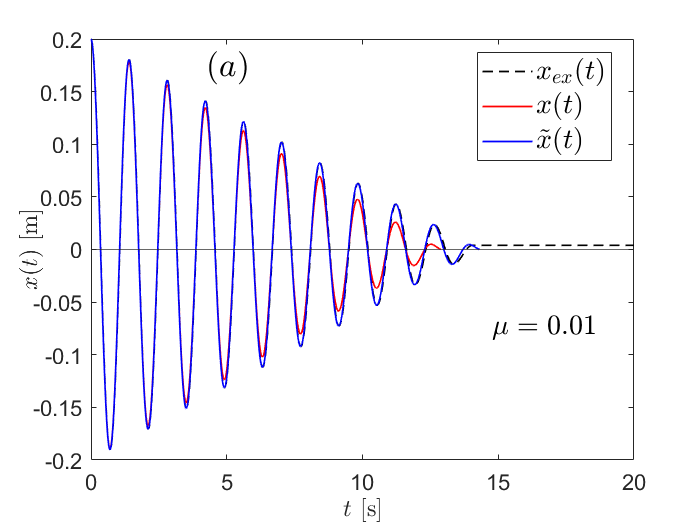
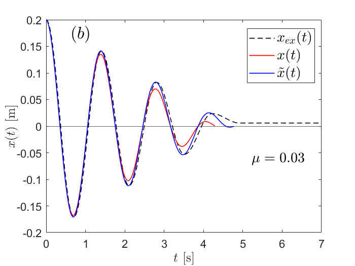
As we noted earlier, solution (47) comes to a stop in equilibrium position at $\tau=\sqrt{2}\omega_{0}x_{0}/(\mu g)$, which in this case amounts to $\tau=12.9\,s$ for $\mu=0.01$, and to $\tau=4.3\,s$ for $\mu=0.03$. In that respect, solution (48) behaves qualitatively the same, i.e. it comes to a stop in equilibrium position at $\tilde{\tau}=\pi\omega_{0}x_{0}/(2\mu g)$, which amounts to $\tilde{\tau}=14.33\,s$ for $\mu=0.01$, and to $\tilde{\tau}=4.78\,s$ for $\mu=0.03$. We read directly from the graph that the exact solution stops at time $\tau_{ex}=14.05\,s$ at displacement $+0.02x_{0}$ for $\mu=0.01$, and at time $\tau_{ex}=4.93\,s$ at displacement $+0.03x_{0}$ for $\mu=0.03$.

We see in Fig. 1 that the solution (48) is a better approximation of the exact solution than our solution (47), especially as the dynamics approaches to a halt. Nevertheless, our solution also describes very well the dynamics of the systems if condition (50) is valid, i.e. our solution shows a linear decay of the amplitude and provides a solid estimate of the duration of the motion. The benefit of our approach is in a less demanding derivation compared to the approach presented in Wang , i.e. even students who have not studied integral calculus can understand it.

VI Air resistance: Comparison of our results with the results of a known method

As in previous section, here we deal with the dynamics that started with initial conditions $(x(0)=x_{0},v(0)=0)$. In that case, our approximate solution of equation (1), with damping force (5), is

$$x(t)=x_{0}\left(1+\frac{C\omega_{0}x_{0}}{2^{\frac{3}{2}}m}t\right)^{-1}\cos(\omega_{0}t)\,.$$ (51)

Equation of motion (1) with damping force (5) is a nonlinear differential equation that cannot be solved analytically. In Wang , amplitude decay in case of weak damping with damping force quadratic in velocity is derived using the approximation that the amplitude remains constant over time intervals of one period in length and using the energy dissipation rate averaged (integrated) over these time intervals. In Wang , it was also shown that the approximate solution thus obtained agrees very well with the experimental data. Therefore, to check the quality of our approach in case of damping quadratic in velocity, we will compare solution (51) with the solution given by the approach introduced in Wang when applied to the system described by equation (1) with damping force (5), i.e. compare (51) with

$$\tilde{x}(t)=x_{0}\left(1+\frac{4C\omega_{0}x_{0}}{3\pi m}t\right)^{-1}\cos(\omega_{0}t)\,.$$ (52)

In Fig. 2 we show the approximate solutions (51) (solid red curve) and (52) (solid blue curve). In both Fig. 1(a) and (b), we use the same values of $m$, $k$, $x_{0}$ and $g$ as in previous section. For the chosen values, condition (46) becomes

$$C\ll 21.21\frac{Ns^{2}}{m^{2}}\,.$$ (53)

In Fig. 2(a) we show the dynamics with $C=0.2\,Ns^{2}/m^{2}$, and in Fig. 2(b) with $C=2\,Ns^{2}/m^{2}$.

Figure 2: Solutions (51) (solid red curve), (52) (solid blue curve), for (a) $C=0.2\,Ns^{2}/m^{2}$ and (b) $C=2\,Ns^{2}/m^{2}$. See text for details.

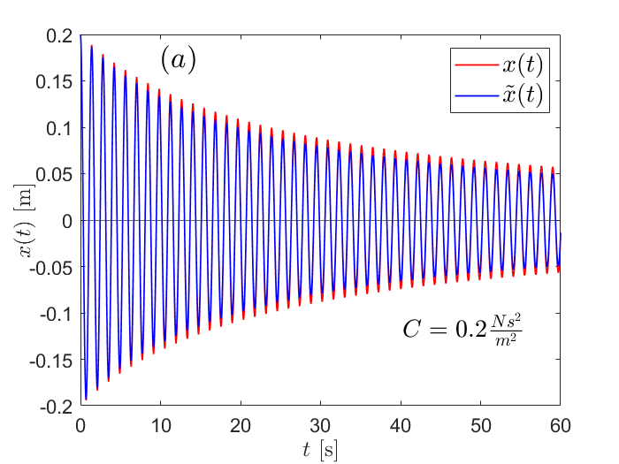
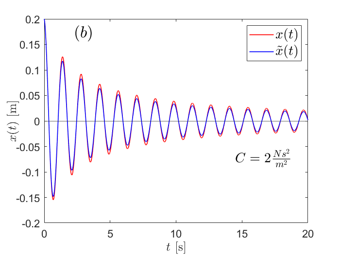
We see in Fig. 2 that our solution (51) agrees well with the solution (52), i.e. it gives only a slightly slower amplitude decay compared to the solution (52). Therefore, along with the approach presented in Wang , our approach can also be used to introduce undergraduate students with the damping quadratic in velocity. In terms of mathematical complexity, a small advantage of our approach, compared to the approach in Wang , is that students don’t need to calculate two integrals, but only one, the one they are typically familiar with in the first year of undergraduate studies. More precisely, for damping quadratic in velocity the approach used in Wang requires solving integrals $\int_{0}^{T_{0}}\sin^{3}(\omega_{0}t)dt$ and $\int_{0}^{t}f^{-2}(t^{\prime})df(t^{\prime})$, while in our approach we don’t need to calculate the first of those two integrals.

VII Discussion and conclusion

In the case of weak damping, for all three damping forces (i.e. for (2), (3) and (5)) we can take $x(t)=A_{0}f(t)\cos(\omega_{0}t+\phi_{0})$ and $v(t)=-\omega_{0}A_{0}f(t)\sin(\omega_{0}t+\phi_{0})$ as approximate forms of displacements and velocities, where $A_{0}$ and $\phi_{0}$ can be determined from initial conditions. If we insert these approximate forms of solutions and $F_{d}(t)\propto v^{n}(t)$, with $n=\{0,1,2\}$, in energy dissipation rate $dE(t)/dt=F_{d}(t)v(t)$ we get

$$m\omega_{0}^{2}A_{0}^{2}f(t)\frac{df(t)}{dt}\propto\omega_{0}^{n+1}A_{0}^{n+1}f^{n+1}(t)\sin^{n+1}(\omega_{0}t+\phi_{0})\,.$$ (54)

From equation (54) we see that in case $n=1$ (damping linear in velocity) amplitude $A_{0}$ can be eliminated (crossed out) from the equation. Thus, we would like to note here that in case $n=1$ our procedure of adding two equations, obtained from energy dissipation rates, can work if we use any two pairs of initial conditions that are phase shifted by $\pi/2$, i.e. if we get equation (54) for the first pair, and the other pair has approximate solution of the form $B_{0}f(t)\cos(\omega_{0}t+\beta_{0})$, the only necessary condition for our procedure to work is that $\beta_{0}=\phi_{0}\pm\pi/2$, but $A_{0}$ and $B_{0}$ may be different. However, when students encounter this topic for the first time, in our opinion it is better to explain the entire procedure to them using two pairs of initial conditions that have the same initial energy, i.e. with $A_{0}=B_{0}$ and $\beta_{0}-\phi_{0}=\pm\pi/2$, for simplicity, as is done in LelasPezer .

For other two types of damping ($n=0$ and $n=2$) the amplitude $A_{0}$ can not be eliminated from equation (54) and our procedure works only if we consider pairs of initial conditions with $A_{0}=B_{0}$ and $\beta_{0}-\phi_{0}=\pm\pi/2$. This is evident from the weak damping conditions (33) and (46) which both depend on initial displacement $x_{0}$, thus initial conditions play an important role in overall dynamics in these cases, while initial conditions do not appear in the weak damping condition (21), i.e. in the case of viscous damping. However, we note here that initial conditions can play an important role also in the case of viscous damping if all values of the damping constant $b$ have to be considered, and not only the weak regime, as is the case in the context of the optimal damping problems Lelas2023 ; Lelas2024 .

If the instructor wants to avoid introducing the sign function (4), the alternative is to use $F_{d}(t)\propto-v^{n+1}(t)/|v(t)|$, with $n=\{0,2\}$, in (3) and (5). In that case $P_{d}(t)\propto-v^{n+2}(t)/|v(t)|$, and it is easy to argue that relations $-v^{2}(t)/|v(t)|=-|v(t)|$ and $-v^{4}(t)/|v(t)|=-|v(t)|^{3}$ are valid. Thus, we get easily the same expressions as by using the sign function in our derivations of approximate amplitudes $f(t)$.

In conclusion, we showed how to obtain a fairly good approximation of the amplitude decay, i.e., of the solutions that describe the dynamics of harmonic oscillator damped with sliding friction and with air resistance. In case of sliding friction, we arrive at the final expression for the amplitude decay using simpler mathematics than is required for the exact solution, and there is no need for integral calculus as in Wang . Thus, for this type of damping our approach is suitable for both first year undergraduates and for high school students. In case of air resistance, we arrive at the final expression for the amplitude decay without the need for averaging over time, i.e. in our approach, we use one integration less compared to the approach in Wang . In this sense, our approach is somewhat easier from the mathematical side than the approach in Wang . We believe that our approach can be useful in teaching first year undergraduates about oscillations with damping quadratic in velocity.

VIII Acknowledgments

This work was supported by the QuantiXLie Center of Excellence, a project co-financed by the Croatian Government and European Union through the European Regional Development Fund, the Competitiveness and Cohesion Operational Programme (Grant No. KK.01.1.1.01.0004).

References

- [1] J.D. Cutnell and K.W. Johnson. Physics. John Wiley & Sons, 2009.
- [2] David Halliday, Robert Resnick, and Jearl Walker. Fundamentals of Physics. John Wiley & Sons, 2013.
- [3] Hugh D. Young and Roger A. Freedman. University Physics with Modern Physics. Pearson, 2020.
- [4] Frank S. Crawford. Waves: Berkeley Physics Course. volume 3. McGraw-Hill, New York, 1968.
- [5] J. A. Rizcallah. Revisiting the coulomb-damped harmonic oscillator. European Journal of Physics, 40(5), aug 2019.
- [6] I. R. Lapidus. Motion of a harmonic oscillator with sliding friction. American Journal of Physics, 38(11):1360––1361, nov 1970.
- [7] A. Marchewka, David. S. Abbott, and R. J. BeichnerKamela. Oscillator damped by a constant-magnitude friction force. American Journal of Physics, 72(4):477––483, apr 2004.
- [8] A. Anastasios Adamopoulosa and N. Adamopoulos. Constant and quadratic damping of free oscillations: easy solutions. International Journal of Mathematical Education in Science and Technology, 53(11):3151–3161, jan 2022.
- [9] M. Kamela. An oscillating system with sliding friction. The Physics Teacher, 45(2):110–113, feb 2007.
- [10] B. R. Jr. Smith. The quadratically damped oscillator: A case study of a non-linear equation of motion. American Journal of Physics, 80(9), sep 2012.
- [11] C. E. Mungan and T. C. Lipscombe. Oscillations of a quadratically damped pendulum. European Journal of Physics, 34(5):1243–1253, jul 2013.
- [12] X. Wang, C. Schmitt, and M. Payne. Oscillations with three damping effects. European Journal of Physics, 23(2):155–164, jan 2002.
- [13] K. Lelas and R. Pezer. Modeling the amplitude and energy decay of a weakly damped harmonic oscillator using the energy dissipation rate and a simple trick. European Journal of Physics, 2024.
- [14] Karlo Lelas, Nikola Poljak, and Dario Jukić. Damped harmonic oscillator revisited: The fastest route to equilibrium. American Journal of Physics, 91(10):767–775, 10 2023.
- [15] K. Lelas and I. Nakić. Optimal damping of vibrating systems: Dependence on initial conditions. Journal of Sound and Vibration, 576:118303, 2024.