Single Antenna Tracking and Localization of RIS-enabled Vehicular Users

Abstract

Reconfigurable Intelligent Surfaces are envisioned to be employed in next generation wireless networks to enhance the communication and radio localization services. In this paper, we propose novel localization and tracking algorithms exploiting reflections through RISs at multiple receivers. We utilize a single antenna transmitter (Tx) and multiple single antenna receivers to estimate the position and the velocity of users (e.g. vehicles) equipped with RISs. Then, we design the RIS phase shifts to separate the signals from different users. The proposed algorithms exploit the geometry information of the signal at the RISs to localize and track the users. We also conduct a comprehensive analysis of the Cramer-Rao lower bound (CRLB) of the localization system. Compared to the time of arrival (ToA)-based localization approach, the proposed method reduces the localization error by a factor up to three. Also, the simulation results show the accuracy of the proposed tracking approach.

I Introduction

With the progress of technology over the last decades, localization and tracking have become one of the necessities in human life. Applications of localization are in navigation of vehicles and robots, emergency services, location-based services in wireless networks, security, etc. Due to the inherent limitations of Global Positioning System (GPS) in indoor environments and outdoor environments with tall buildings, the attention of the researchers has been turned to the radio localization, motivating a huge interest in the integration of localization, sensing and communication (ISAC) in future wireless systems [1, 2, 3, 4, 5]. The main challenge of radio localization systems is to simultaneously achieve wide coverage and high accuracy, while using the minimum number of Txs/Rxs [6, 7]. A promising technology to help overcome this challenge is RIS.

An RIS is a planner array composed of passive reflecting elements with dynamically configurable phase shifts. RISs have been used not only to enhance wireless communication performance [8, 9, 10, 11], but also to boost radio localization capabilities [12, 13]. In many of the localization researches the RISs are considered as anchor nodes with known location. The deployment of RISs to improve the accuracy is one of the initial problems explored in this context. In this regard, enhancing the localization accuracy in a system equipped by a single antenna Tx/Rx and multi-antenna Rx/Tx has been examined in [14, 15, 16, 17]. Also, in [18, 19, 20], this problem is investigated in a system equipped with multi-antenna Tx and Rx. Moreover, the authors in [21, 22, 23, 24] investigated the problem of localizing a single antenna user equipment (UE) employing a single antenna Tx. Another challenge is employing RISs to localize the UEs without any access point [25, 26]. Also, the problem of localizing unknown location Txs and Rxs has been investigated in [27, 28]. The enhancement of the tracking accuracy is another role for the RISs, which is studied in [29, 30].

However, all of these works assume that the location of the RIS is known and use it as anchor. But, what if the RISs are deployed on vehicles and we are uncertain about their precise location? In such situations, we need to estimate the location of the RIS itself. There are a limited number of studies that address the RIS localization problem [31, 32, 33, 34, 35]. In [31], localization of RIS-equipped UEs using a Tx and multiple Rxs is considered, where, for each RIS the time difference of arrival (TDoA) of the path including the RIS and each Rx and the direct path between the Tx and Rx is measured and the location of the RIS is estimated by minimizing the maximum likelihood (ML) for the TDoAs. Thus, at least three Rxs are required to localize the RISs in this work. In [32], the problem of localizing an RIS in the near field is investigated. In this article, a ML estimation problem is defined to localize the RIS using one Tx and one Rx. In [33, 34, 35], a multiple-input multiple-output (MIMO) Rx is employed to estimate the location of the RIS and the Tx (user). To do this, in [33] a prior information about the locations is utilized, while in [34, 35] active and hybrid RISs are employed, respectively.

However, these works mostly consider static scenarios which is not suitable for mobile RIS such as vehicles equipped with RIS in smart transportation systems where the mobility features such as Doppler effect can not be ignored.To the best of our knowledge, this paper is the first study of the RIS tracking problem.

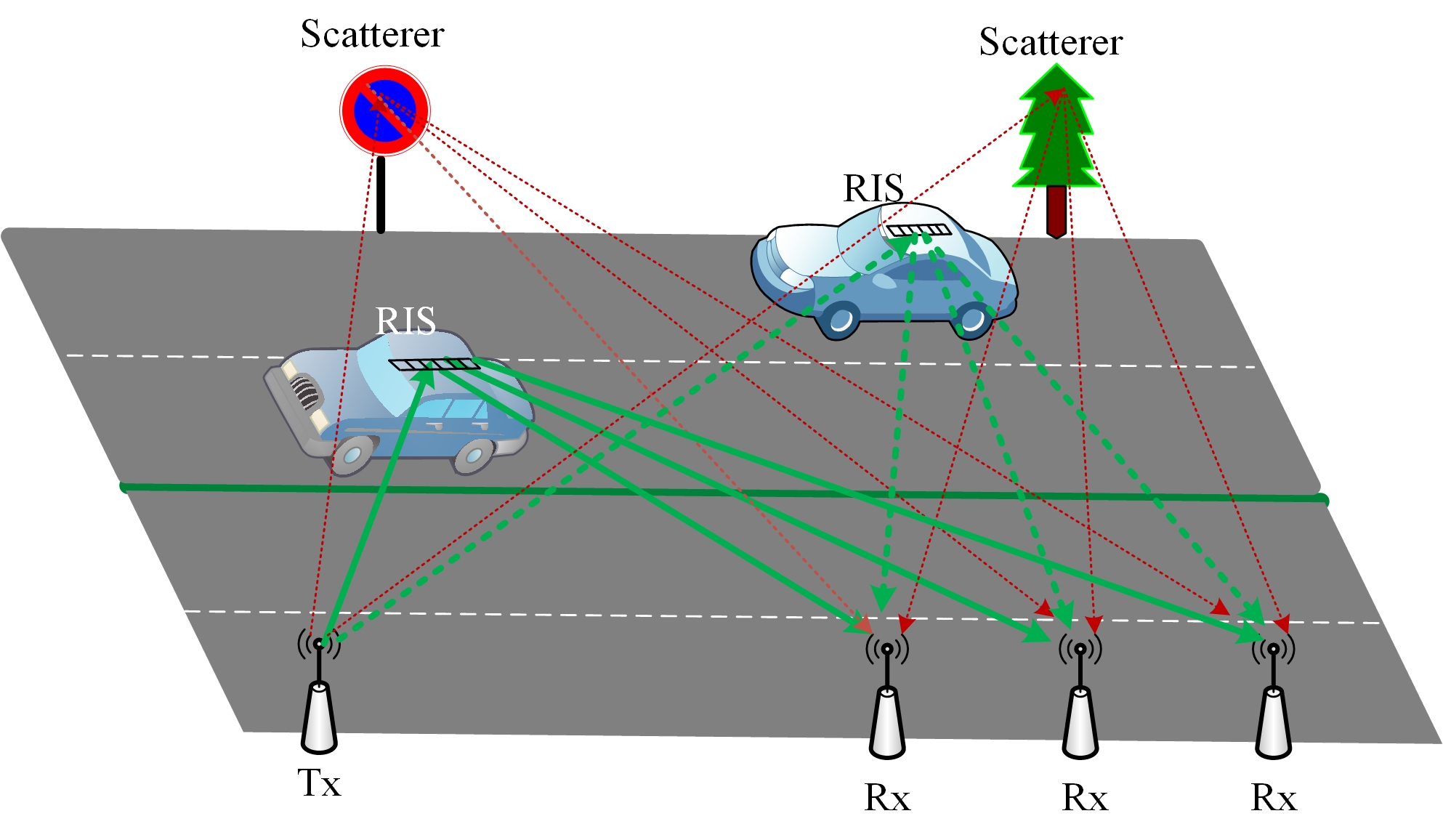
Figure 1: A capture of the considered scenario, as $N_{\mathrm{r}}=3$, $K=2$ and $L=2$.

TABLE I: The Key Differences Between This Work and the Literature

	Tracking	Single Antenna Tx and Rx	Doppler Effect	Simultaneous Tracking /Localization of Multiple Targets	CRLB Analysis	Scatterers	Unknown Location RIS	Unknown Location Tx/Rx
[14]	N	N	N	N	Y	N	N	Y
[36]	N	N	N	Y	N	Y	N	Y
[20]	N	N	N	N	Y	Y	N	Y
[30]	Y	N	N	Y	Y	N	N	Y
[32]	N	Y	N	N	Y	N	Y	N
[31]	N	Y	N	Y	Y	N	Y	N
[33]	N	N	N	Y	Y	N	Y	Y
[34]	N	N	N	N	Y	N	Y	Y
[35]	N	N	N	N	Y	N	Y	Y
This work	Y	Y	Y	Y	Y	Y	Y	N

In this paper, we study the problem of tracking the trajectory and speed of multiple UEs (e.g., vehicles) each equipped with an RIS, in the presence of the scatters, employing a single antenna Tx and multiple single antenna Rxs. In this regard, first we propose a novel localization algorithm to estimate the initial location of the RISs. Then, we propose an efficient algorithm for simultaneous tracking of multiple RISs. Table I summarizes the key differences between this work and the literature. The contributions of this paper are summarized as follows.

• We propose an algorithm to simultaneously track the trajectory and speed of multiple RISs based on extended Kalman filtering (EKF). The proposed approach leverages the ToA of the paths and information about the geometry of the reflected signals at the RIS.

• By estimating the ToAs and sum cosines of the angle of arrival (AoA) and angle of departure (AoD) at each RIS as the measurement parameters, we also propose an RIS localization algorithm to initialize the tracking. To do so, we design the phase shifts to extract the signals reflected by various RISs and discriminate them from those reflected by scatterers at each Rx. Thanks to the exploited geometric information, the proposed localization approach works even with a single Rx.

• We derive the CRLB and demonstrate the behaviour of Position Error Bound (PEB) in terms of the distance between the RIS and the line between the Tx and Rx.

The rest of the paper is organized as follows. In Section II, we present the system model. In Section III, the phase shifts design approach, measurement parameters and the proposed localization approach are introduced. Section IV provides the proposed tracking approach. The CRLB of the localization system is derived in Section V. Section VI presents the simulation results, and Section VII concludes the paper.

Notations. The vectors and the matrices are denoted with boldface letters and boldface capital letters, respectively. For matrix $\bf A$, $\mathrm{tr}\{\mathbf{A}\}$ denotes the trace of the matrix and $\mathbf{A}^{T}$, $\mathbf{A}^{H}$, $\mathbf{A}^{*}$, and $[\bf A]_{i,j}$ are the transpose, Hermitian, conjugate and element $(i,j)$ of the matrix, respectively. Also, for vector $\mathbf{u}$, $[\mathbf{u}]_{i}$ shows the $i^{\mathrm{th}}$ element of this vector, and for vectors $\mathbf{u}$ and $\mathbf{v}$, $\mathbf{u}\odot\mathbf{v}$ represents the element-wise multiplication of the vectors. Moreover, operators $|.|$ and $\parallel.\parallel$ return the absolute value of scalars and the norm of vectors, respectively.

II System Model

We consider a localization system comprising a single antenna Tx and $N_{\mathrm{r}}$ single antenna Rxs deployed in an environment with $L$ scatterers (as in Fig. 1). We consider $K$ users (e.g., vehicles) with unknown locations, each equipped with a linear RIS[37, 38, 39, 40], whose locations trajectory and speed are to be estimated. We denote the location of the Tx, the $n_{\mathrm{r}}^{\mathrm{th}}$ Rx and $k^{\mathrm{th}}$ RIS with $\mathbf{p}_{{}_{\rm t}}$, $\mathbf{p}_{{}_{\mathrm{r},n_{r}}}$, and $\mathbf{p}_{{}_{k}}$, respectively, as shown in Fig. 2. Moreover, $\phi_{k}$, $\theta_{k,n_{\mathrm{r}}}$ and $\psi_{k,n_{\mathrm{r}}}$ represent the AoA of the path between the Tx and the $k^{\mathrm{th}}$ RIS and the AoD of the path between the $k^{\mathrm{th}}$ RIS and the $n_{\mathrm{r}}^{\mathrm{th}}$ Rx, and the orientation of the $k^{\mathrm{th}}$ RIS with respect to the line between the Tx and the $n_{\mathrm{r}}^{\mathrm{th}}$ Rx, respectively. Furthermore, the steering vectors of the AoA and AoDs of the $k^{\mathrm{th}}$ RIS are denoted as $\mathbf{a}(\phi_{k})$ and $\mathbf{a}(\theta_{k,n_{\mathrm{r}}})$ for $n_{\mathrm{r}}\in\mathcal{N}_{\mathrm{r}}\triangleq\{1,\dots,n_{\mathrm{r}}\}$, where

$$\mathbf{a}(\psi)=[1,e^{j\frac{2\pi}{\lambda}d\cos\psi},\dots,e^{j\frac{2\pi}{\lambda}(M-1)d\cos\psi}]^{T},$$ (1)

in which $M$ is the number of the RIS elements.

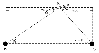
Figure 2: Representation of locations and AoA and AoD in a scenario including the Tx, the $n^{\mathrm{th}}$ Rx, and the $k^{\mathrm{th}}$ RIS.

The Tx sends an orthogonal frequency-division multiplexing (OFDM) signal with $N$ sub-carriers for $\bar{T}$ times. At the $n_{\mathrm{r}}^{\mathrm{th}}$ Rx, after removing the Cyclic Prefix (CP) and applying fast Fourier transform (FFT), the received signal can be written as

$$\mathbf{y}_{n_{\mathrm{r}},\bar{t}}= \sqrt{E_{s}}\sum\limits_{k=1}^{K}g_{k,n_{\mathrm{r}}}\mathbf{d}(\tau_{k,n_{\mathrm{r}}})\mathbf{a}(\theta_{k,n_{\mathrm{r}}})^{T}\mbox{\boldmath{$\Phi$}}_{k}(\bar{t})\mathbf{a}(\phi_{k})$$

$$\times e^{j2\pi f_{{}_{\mathrm{d},k,n_{\mathrm{r}}}}T_{\mathrm{d}}(\bar{t}-1)}+\sqrt{E_{s}}\sum\limits_{\ell=0}^{L}{g}^{\prime}_{\ell,n_{\mathrm{r}}}\mathbf{d}({\tau}^{\prime}_{\ell,n_{\mathrm{r}}})+\mathbf{w}_{n_{\mathrm{r}},\bar{t}},$$

$$\forall\bar{t}\in\{1,2,\cdots,\bar{T}\},$$ (2)

where $E_{s}$ is the energy of the transmit signal,

$$\mathbf{d}(\tau)=[1,e^{j2\pi\Delta_{f}\tau},\dots,e^{j2\pi(N-1)\Delta_{f}\tau}]^{T},$$

$\mbox{\boldmath{$\Phi$}}_{k}(\bar{t})\in\mathbb{C}^{M\times M}$ is the phase profile matrix of the $k^{\mathrm{th}}$ RIS at the $\bar{t}^{\mathrm{th}}$ transmission, and $\mathbf{w}_{n_{\mathrm{r}},\bar{t}}$ is the additive white Gaussian noise (AWGN) vector at the $n_{\mathrm{r}}^{\mathrm{th}}$ Rx with power spectral density $N_{0}$. Also, $g_{k,n_{\mathrm{r}}}$ and $\tau_{k,n_{\mathrm{r}}}$ are the channel amplitude and the delay of the path between the Tx and the $n_{\mathrm{r}}^{\mathrm{th}}$ Rx including the $k^{\mathrm{th}}$ RIS, respectively, and ${g}^{\prime}_{\ell,n_{\mathrm{r}}}$ and ${\tau}^{\prime}_{\ell,n_{\mathrm{r}}}$ are the channel amplitude and the delay of the path between the Tx and the $n_{\mathrm{r}}^{\mathrm{th}}$ Rx including the $\ell^{th\rm}$ scatterer, respectively ($\ell=0$ is corresponding to the direct paths between the Tx and Rxs). Additionally, $f_{{}_{\mathrm{d},k,n_{\mathrm{r}}}}=v_{k}(\cos\phi_{k,n_{\mathrm{r}}}+\cos\theta_{k,n_{\mathrm{r}}})f_{c}/c$ is the Doppler frequency of the signal reflected by the $k^{\mathrm{th}}$ RIS and received by the $n_{\mathrm{r}}^{\mathrm{th}}$ Rx in which $v_{k}$ is the velocity of the $k^{\mathrm{th}}$ RIS, $f_{c}$ is the carrier frequency, $c$ is the speed of light, and $T_{d}$ is the symbol duration of the OFDM signal plus duration of the CP.

III Proposed Localization Approach

In order to investigate the tracking problem, first we need to consider measurement parameters and also design a localization approach to estimate the initial location of the RISs. In this regard, in this section, we propose a phase shift design approach and estimate the ToA and the Doppler frequency of the paths between the Tx and Rxs including the $k^{\mathrm{th}}$ RIS as well as parameter $\alpha_{k,n_{\mathrm{r}}}\triangleq\cos\phi_{k}+\cos\theta_{k,n_{\mathrm{r}}}$, for $k\in\mathcal{K}\triangleq\{1,\dots,K\}$ and $n_{\mathrm{r}}\in\mathcal{N}_{\mathrm{r}}$. Then, using these parameters we define a least square (LS) problem to localize the $k^{\mathrm{th}}$ RIS. We also will employ the ToAs and $\alpha_{k,n_{\mathrm{r}}}$s as the measurement parameters to propose the tracking algorithm in the next section.

III-A Phase shift and observation vector design

We have three purposes in the design of RIS phase shifts: (i) Be able to eliminate the effect of scatterers. (ii) Be able to separate the signals of different RISs. (iii) Be able to estimate the value of $\alpha_{k,n_{\mathrm{r}}}$. In this part, we design the phase shifts of the RISs in order to separate the signals reflected by various RISs at the Rxs and discriminate them from the scatterers. This enables simultaneous localization and tracking of multiple RISs from the received signals. To do this, we divide $\bar{T}$ into $N_{T}$ intervals each including $T$ slots (i.e., $\bar{T}=N_{T}T$) and for $n_{T}\in\mathcal{N}_{T}\triangleq\{1,\dots,N_{T}\}$ consider $\mathbf{Y}_{n_{\mathrm{r}},n_{T}}\in\mathbb{C}^{N\times T}$ as the matrix form of the signals received by the $n_{\mathrm{r}}^{\mathrm{th}}$ Rx at the slots of this interval. Thus,

$$\mathbf{Y}_{n_{\mathrm{r}},n_{T}}= \sqrt{E_{s}}\sum\limits_{k=1}^{K}g_{k,n_{\mathrm{r}}}e^{j2\pi f_{{}_{\mathrm{d},k,n_{\mathrm{r}}}}(n_{T}-1)T_{\mathrm{d}}T}$$

$$\times\mathbf{d}(\tau_{k,n_{\mathrm{r}}})[\mathbf{u}_{n_{T}}(\theta_{k,n_{\mathrm{r}}},\phi_{k})\odot\mathbf{d}_{\mathrm{d}}(f_{{}_{\mathrm{d},k,n_{\mathrm{r}}}})]^{T}$$

$$+\sqrt{E_{s}}\sum\limits_{\ell=0}^{L}g_{\ell,n_{\mathrm{r}}}^{\prime}\mathbf{d}(\tau_{\ell,n_{\mathrm{r}}}^{\prime})1_{T}^{T}+\mathbf{W}_{n_{\mathrm{r}},n_{T}},$$ (3)

in which $[\mathbf{u}_{n_{T}}(\theta_{k,n_{\mathrm{r}}},\phi_{k})]_{t}=\mathbf{a}(\theta_{k,n_{\mathrm{r}}})^{T}\mbox{\boldmath{$\Omega$}}_{k}(t,n_{T})\mathbf{a}(\phi_{k})$, where $\mbox{\boldmath{$\Omega$}}_{k}(t,n_{T})=\mbox{\boldmath{$\Phi$}}_{k}((n_{T}-1)T+t)$ for $t\in\mathcal{T}\triangleq\{1,\dots,T\}$, $\mathbf{d}_{\mathrm{d}}(f_{{}_{\mathrm{d},k,n_{\mathrm{r}}}})=[1\ e^{j2\pi f_{{}_{\mathrm{d},k,n_{\mathrm{r}}}}T_{\mathrm{d}}}\dots e^{j2\pi f_{{}_{\mathrm{d},k,n_{\mathrm{r}}}}T_{\mathrm{d}}(T-1)}]^{T}$, and $\mathbf{W}_{n_{\mathrm{r}},n_{T}}$ is the AWGN matrix with variance $\sigma^{2}_{\mathbf{W}}=\Delta_{f}N_{0}$ in which $N_{0}$ is the power spectral density.

We design the phase profile matrix of the $k^{\mathrm{th}}$ RIS as $\mbox{\boldmath{$\Omega$}}_{k}(t,n_{T})=\omega_{k,t}\mbox{\boldmath{$\Omega$}}_{k}^{(n_{T})}$ for $t\in\mathcal{T}$ and $n_{T}\in\mathcal{N}_{T}$, where matrix $\mbox{\boldmath{$\Omega$}}_{k}^{(n_{T})}$ is constant during each $T$ transmissions. We set vectors $\mbox{\boldmath{$\omega$}}_{k}=[\omega_{k,1},\dots,\omega_{k,T}]^{T}$, $k\in\mathcal{K}$, such that $\forall\ t\in\{1,...,T/2\}$, $\omega_{k,2t}=-\omega_{k,2t-1}$ and vectors $\mbox{\boldmath{$\gamma$}}_{k}=[\omega_{k,1},\omega_{k,3},\dots,\omega_{k,T-1}]^{T}$, for $k\in\mathcal{K}$ be orthogonal to each other. To satisfy the orthogonality, vectors $\mbox{\boldmath{$\gamma$}}_{k}$ can be chosen from the set of the columns of the FFT matrix with dimensions $T/2$. In practice, to not to be have to update the dimensions of the FFT matrix when the number of the RISs increases, we consider a maximum number for the RISs and set the dimensions of the FFT matrix by this number.

Now, let us separate matrix $\mathbf{Y}_{n_{\mathrm{r}},n_{T}}$ into sub-matrices $\mathbf{Y}_{n_{\mathrm{r}},n_{T},o}$ and $\mathbf{Y}_{n_{\mathrm{r}},n_{T},e}$ that contain the odd and even columns, respectively. Considering that the scatterers are fixed during transmissions and thus the terms of the scatterers are the same in the odd and even columns, while by designing $\omega_{k,2t}=-\omega_{k,2t-1}$ for $t\in\{1,...,T/2\}$, the terms corresponding to the RISs are opposite, we can remove the contributions of the scatterers by computing

$$\mathbf{Y}_{n_{\mathrm{r}},n_{T}}^{\prime}=\frac{1}{2}(\mathbf{Y}_{n_{\mathrm{r}},n_{T},o}-\mathbf{Y}_{n_{\mathrm{r}},n_{T},e}).$$ (4)

III-B Joint Estimation of $\tau_{k,n_{\mathrm{r}}}$ and $f_{{}_{\mathrm{d},k,n_{\mathrm{r}}}}$

To estimate $\tau_{k,n_{\mathrm{r}}}$ and $f_{{}_{\mathrm{d},k,n_{\mathrm{r}}}}$, we first extract the signal of the $k^{\mathrm{th}}$ RIS. Neglecting the effect of the Doppler shifts, considering the orthogonality of $\mbox{\boldmath{$\gamma$}}_{k}$s, we extract the $n_{T}^{\mathrm{th}}$ signal vector received through the path including the $k^{\mathrm{th}}$ RIS, by computing $\mathbf{r}_{k,n_{\mathrm{r}},n_{T}}=\frac{2}{T}\mathbf{Y}_{n_{\mathrm{r}},n_{T}}^{\prime}\mbox{\boldmath{$\gamma$}}_{k}^{*}$. Thus,

$$\mathbf{r}_{k,n_{\mathrm{r}},n_{T}}=\sqrt{E}_{s}\ g_{k,n_{\mathrm{r}}}\mathbf{d}(\tau_{k,n_{\mathrm{r}}})\mathbf{a}(\theta_{k,n_{\mathrm{r}}})^{T}\mbox{\boldmath{$\Omega$}}_{k}^{(n_{T})}\mathbf{a}(\phi_{k})\times$$

$$e^{j2\pi f_{{}_{\mathrm{d},k,n_{\mathrm{r}}}}(n_{T}-1)T_{\mathrm{d}}T}\sum_{t=1}^{T/2}\left(1+e^{j2\pi f_{{}_{\mathrm{d},k,n_{\mathrm{r}}}}T_{\mathrm{d}}(t-1)}\right)+\mathbf{z}_{k,n_{\mathrm{r}},n_{T}},$$ (5)

in which $\mathbf{z}_{k,n_{\mathrm{r}},n_{T}}=\frac{2}{T}\mathbf{W}_{n_{\mathrm{r}},n_{T}}^{\prime}\mbox{\boldmath{$\gamma$}}_{k}^{*}+\mathcal{I}_{k,n_{\mathrm{r}},n_{T}}$, where $\mathcal{I}_{k,n_{\mathrm{r}},n_{T}}$ is the leakage of the signals corresponding to the other RISs. We must note that neglecting the Doppler shifts to be able to exactly extract the signal reflected by each RIS as (5), $T$ should satisfy $K\leq T/2$.

Now, considering the design of matrix $\mbox{\boldmath{$\Omega$}}_{k}^{(n_{T})}$ in which for $n_{T}\in\{1,\dots,N_{T}/2\}$ and $m\neq 2$, $\Omega_{k,m,m}^{(2n_{T}-1)}=\Omega_{k,m,m}^{(2n_{T})}$ and $\Omega_{k,2,2}^{(2n_{T}-1)}\neq\Omega_{k,2,2}^{(2n_{T})}$ (See Section III-C), we subtract the consecutive vectors i.e., $\mathbf{r}_{k,n_{\mathrm{r}},2n_{T}-1}$ and $\mathbf{r}_{k,n_{\mathrm{r}},2n_{T}}$ for $n_{T}\in\{1,\dots,N_{T}/2\}$ to obtain a set of vectors that their phase shifts compared to each other is just the Doppler shift as blow

$$\mathbf{r}^{\prime}_{k,n_{\mathrm{r}},n_{T}}=\mathbf{r}_{k,n_{\mathrm{r}},2n_{T}-1}-\mathbf{r}_{k,n_{\mathrm{r}},2n_{T}},\forall n_{T}\in\{1,\dots,N_{T}/2\}.$$ (6)

Then, we construct matrix $\mathbf{R}_{k,n_{\mathrm{r}}}=[\mathbf{r}^{\prime}_{k,n_{\mathrm{r}},1}\dots\mathbf{r}^{\prime}_{k,n_{\mathrm{r}},N_{T}/2}]\in\mathcal{C}^{N\times N_{T}/2}$ in which the difference of the phase shifts of the consecutive elements on each column is $2\pi\Delta_{f}\tau_{k,n_{\mathrm{r}}}$ and the difference of the phase shifts the consecutive elements on each row is equal to $4\pi f_{{}_{\mathrm{d},k,n_{\mathrm{r}}}}T_{\mathrm{d}}T$. We aim to employ 2DFFT of signal $\mathbf{r}_{k,n_{\mathrm{r}},n_{T}}$ to jointly estimate $\tau{k,n_{\mathrm{r}}}$ and $f_{{}_{\mathrm{d},k,n_{\mathrm{r}}}}$. But, the challenge is that the sign of $f_{{}_{\mathrm{d},k,n_{\mathrm{r}}}}$ is unknown. To solve this problem, assuming that $|4\pi f_{{}_{\mathrm{d},k,n_{\mathrm{r}}}}T_{\mathrm{d}}T|<2\pi-|4\pi f_{{}_{\mathrm{d},k,n_{\mathrm{r}}}}T_{\mathrm{d}}T|$, we propose algorithm 1 to jointly estimate $\tau_{k,n_{\mathrm{r}}}$ and $f_{{}_{\mathrm{d},k,n_{\mathrm{r}}}}$. In this algorithm, $\mathbf{F}_{\tau}\in\mathcal{C}^{N_{f,\tau}\times N}$ and $\mathbf{F}_{f_{{}_{\mathrm{d}}},1}\in\mathcal{C}^{N_{f,f_{{}_{\mathrm{d}}}}\times N_{T}/2}$ are FFT matrices, and $\mathbf{F}_{f_{{}_{\mathrm{d}}},2}\in\mathcal{C}^{N_{f,f_{{}_{\mathrm{d}}}}\times N_{T}/2}$ is an IFFT matrix. In this algorithm, we use this subject that if we one time estimate $f_{{}_{\mathrm{d},k,n_{\mathrm{r}}}}$ employing the FFT matrix and one time with IFFT matrix, the estimated values satisfy

$$|4\pi\hat{f}_{{}_{\mathrm{d},k,n_{\mathrm{r}},1}}T_{\mathrm{d}}T|=2\pi-|4\pi\hat{f}_{{}_{\mathrm{d},k,n_{\mathrm{r}},2}}T_{\mathrm{d}}T|.$$

Algorithm 1 Proposed Doppler frequency and ToA Estimation Scheme

1:  for $n_{\mathrm{r}}=1$ to $N_{\mathrm{r}}$ do

2:     for $k=1$ to $K$ do

3:        Set

$$[n_{1,\tau}^{*},n_{1,f_{{}_{\mathrm{d}}}}^{*}]=\arg\max\left|\left[\mathbf{F}_{\tau}\mathbf{R}_{k,n_{\mathrm{r}}}\mathbf{F}_{f_{{}_{\mathrm{d}}},1}^{T}\right]_{n_{1,\tau},n_{1,f_{{}_{\mathrm{d}}}}}\right|.$$

4:        Compute $\hat{\tau}_{k,n_{\mathrm{r}}}=(n_{1,\tau}^{*}-1)/(N_{F_{\tau}}\Delta_{f})$ and $\hat{f}_{{}_{\mathrm{d},k,n_{\mathrm{r}},1}}=(2n_{1,f_{{}_{\mathrm{d}}}}^{*}-1)c/(2TT_{\mathrm{d}}f_{c})$.

5:        Set

$$[n_{2,\tau}^{*},n_{2,f_{{}_{\mathrm{d}}}}^{*}]=\arg\max\left|\left[\mathbf{F}_{\tau}\mathbf{R}_{k,n_{\mathrm{r}}}\mathbf{F}_{f_{{}_{\mathrm{d}}},2}^{T}\right]_{n_{2,\tau},n_{1,f_{{}_{\mathrm{d}}}}}\right|.$$

6:        Compute $\hat{f}_{{}_{\mathrm{d},k,n_{\mathrm{r}},2}}=-(2n_{2,f_{{}_{\mathrm{d}}}}^{*}-1)c/(2TT_{\mathrm{d}}f_{c})$.

7:        if $|\hat{f}_{{}_{\mathrm{d},k,n_{\mathrm{r}},1}}|<|\hat{f}_{{}_{\mathrm{d},k,n_{\mathrm{r}},2}}|$ then

8:           $\hat{f}_{{}_{\mathrm{d},k,n_{\mathrm{r}}}}=\hat{f}_{{}_{\mathrm{d},k,n_{\mathrm{r}},1}}$.

9:        else

10:           $\hat{f}_{{}_{\mathrm{d},k,n_{\mathrm{r}}}}=\hat{f}_{{}_{\mathrm{d},k,n_{\mathrm{r}},2}}$.

11:        end if

12:     end for

13:  end for

III-C Estimation of $\alpha_{k,n_{\mathrm{r}}}$

In order to estimate $\alpha_{k,n_{\mathrm{r}}}$, we first remove the effect of ${f}_{d,k,n_{\mathrm{r}}}$ and $\tau_{k,n_{\mathrm{r}}}$. To eliminate the effect of Doppler shifts, for each $k\in\mathcal{K}$, $n_{T}\in\mathcal{N}_{T}$ and $n_{\mathrm{r}}\in\mathcal{N}_{\mathrm{r}}$, we construct semi-orthogonal vectors $\mbox{\boldmath{$\gamma$}}_{k,n_{\mathrm{r}},n_{T}}$, by pointwise multiplication of vectors $\mbox{\boldmath{$\gamma$}}_{k}$s and vectors

$$e^{j2\pi\hat{f}_{{}_{\mathrm{d},k,n_{\mathrm{r}}}}T_{\mathrm{d}}T(n_{T}-1)}\times\left[(1+e^{j2\pi\hat{f}_{{}_{\mathrm{d},k,n_{\mathrm{r}}}}T_{\mathrm{d}}}),\dots,\right.$$

$$\left.(e^{j2\pi\hat{f}_{{}_{\mathrm{d},k,n_{\mathrm{r}}}}T_{\mathrm{d}}(T/2-1)}+e^{j2\pi\hat{f}_{{}_{\mathrm{d},k,n_{\mathrm{r}}}}T_{\mathrm{d}}T/2})\right]^{T},$$

for $k\in\mathcal{K}$ . Then, we simultaneously extract the signal of the $k^{\mathrm{th}}$ RIS and remove the effect of the Doppler shift and $\tau_{k,n_{\mathrm{r}}}$ by obtaining

$$\mathrm{r}_{k,n_{\mathrm{r}},n_{T}}^{\prime\prime} =\frac{2}{T}(\mathbf{Y}_{n_{\mathrm{r}},n_{T}}^{\prime}\mbox{\boldmath{$\gamma$}}_{k,n_{\mathrm{r}},n_{T}})\odot\mathbf{d}(\hat{\tau}_{k,n_{\mathrm{r}}})$$ (7)

$$\simeq s_{k,n_{\mathrm{r}},n_{T}}1_{N}+\mathbf{z}_{k,n_{\mathrm{r}},n_{T}}^{\prime},$$

in which $s_{k,n_{\mathrm{r}},n_{T}}\triangleq\sum_{m=1}^{M}\sqrt{E}_{s}g_{k,n_{\mathrm{r}}}\Omega_{k,m,m}^{(n_{T})}e^{j\frac{2\pi}{\lambda}(m-1)d\alpha_{k,n_{\mathrm{r}}}}$ and $\mathbf{z}_{k,n_{\mathrm{r}},n_{T}}^{\prime}$ the AWGN vector.

Regarding invariance property of the ML estimation approach, we first estimate $s_{k,n_{\mathrm{r}},n_{T}}$, and then use it to obtain the estimated value of $\alpha_{k,n_{\mathrm{r}}}$. The ML estimation of $s_{k,n_{\mathrm{r}},n_{T}}$ for $n_{T}\in\mathcal{N}_{T}$ and $n_{\mathrm{r}}\in\mathcal{N}_{\mathrm{r}}$ is

$$\hat{s}_{k,n_{\mathrm{r}},n_{T}}=\frac{1}{N}\sum_{n=1}^{N}[\mathbf{r}_{k,n_{\mathrm{r}},n_{T}}^{\prime\prime}]_{n}.$$ (8)

Now, for $n_{\mathrm{r}}\in\mathcal{N}_{\mathrm{r}}$ we can obtain $\hat{\alpha}_{k,n_{\mathrm{r}}}$, by solving the following system of non-linear equations

$$\sum_{m=1}^{M}\sqrt{E}_{s}g_{k,n_{\mathrm{r}}}\Omega_{k,m,m}^{(N_{T})}e^{j\frac{2\pi}{\lambda}(m-1)d\alpha_{k,n_{\mathrm{r}}}}=\hat{s}_{k,n_{\mathrm{r}},n_{T}},\forall n_{T}\in\mathcal{N}_{T}.$$ (9)

Regarding the degree of each equation in terms of $e^{j\frac{2\pi}{\lambda}d\alpha_{k,n_{\mathrm{r}}}}$, there exist up to $M-1$ distinct values for $\alpha_{k,n_{\mathrm{r}}}$ in each interval of length $\frac{\lambda}{d}$ satisfying this equation system. Consequently, we generally have ambiguity to estimate the correct value of $\alpha_{k,n_{\mathrm{r}}}$. To address this challenge, we design $\Omega_{k,m,m}^{(n_{T})}$ for $n_{T}\in\mathcal{N}_{T}$ and $m\in\{2,\dots,M\}$ and employ the elimination approach such that the correct value of $\alpha_{k,n_{\mathrm{r}}}$ is distinguishable. For simplicity, we perform this task in such a way that only one of the powers of $e^{j\frac{2\pi}{\lambda}d\alpha_{k,n_{\mathrm{r}}}}$ remains.

Considering that the RISs can have orientation generally $-2<\alpha_{k,n_{\mathrm{r}}}<2$. Thus, assuming that $d=\frac{\lambda}{L}$, the value of $\frac{2\pi}{\lambda}(m-1)d\alpha_{k,n_{\mathrm{r}}}$ is in the range $[-(m-1)\frac{\pi}{L},(m-1)\frac{\pi}{L}]$. Therefore, the remained exponent of $e^{j\frac{2\pi}{\lambda}d\alpha_{k,n_{\mathrm{r}}}}$ ($M^{\prime}$) should be equal or less than $L$, where $L\geq 4$ to ensure that $\frac{2\pi}{\lambda}M^{\prime}d\alpha_{k,n_{\mathrm{r}}}$ is in $(-\pi,\pi)$ and thus the correct value of $\alpha_{k,n_{\mathrm{r}}}$ is distinguishable. To ensure that our system works for all values of $L$ that satisfy this constraint, we design the phase shifts such that for $n_{T}\in\{1,\dots,N_{T}/2\}$ and $m\neq 2$, $\Omega_{k,m,m}^{(2n_{T}-1)}=\Omega_{k,m,m}^{(2n_{T})}$ and $\Omega_{k,2,2}^{(2n_{T}-1)}\neq\Omega_{k,2,2}^{(2n_{T})}$. Thus, subtracting the consecutive equations in (9), we obtain the following system of equations

$$g_{k,n_{\mathrm{r}}}e^{j\frac{2\pi d}{\lambda}\alpha_{k,n_{\mathrm{r}}}}=\frac{1}{\Omega_{k,2,2}^{(N_{T}-1)}-\Omega_{k,2,2}^{(N_{T})}}(\hat{s}_{k,n_{\mathrm{r}},n_{T}-1}-\hat{s}_{k,n_{\mathrm{r}},n_{T}}),$$

$$\ n_{T}\in\{2,\dots,N_{T}\}.$$ (10)

Then, we formulate the following LS problem to estimate $\alpha_{k,n_{\mathrm{r}}}$

$$\min_{\alpha_{k,n_{\mathrm{r}}}\in\mathbb{R}}\sum_{n_{T}=1}^{N_{T}/2}\left|g_{k,n_{\mathrm{r}}}e^{j\frac{2\pi d}{\lambda}\alpha_{k,n_{\mathrm{r}}}}-\frac{\hat{s}_{k,n_{\mathrm{r}},2n_{T}-1}-\hat{s}_{k,n_{\mathrm{r}},2n_{T}}}{\Omega_{k,2,2}^{(2n_{T}-1)}-\Omega_{k,2,2}^{(2n_{T})}}\right|^{2},$$ (11)

and thus, the optimal value of $\alpha_{k,n_{\mathrm{r}}}$ can be derived as

$$\hat{\alpha}_{k,n_{\mathrm{r}}}=\frac{\lambda}{2\pi d}\arg\left(\frac{1}{N_{T}}\sum_{n_{T}=1}^{N_{T}/2}\frac{\hat{s}_{k,n_{\mathrm{r}},2n_{T}-1}-\hat{s}_{k,n_{\mathrm{r}},2n_{T}}}{\Omega_{k,2,2}^{(2n_{T}-1)}-\Omega_{k,2,2}^{(2n_{T})}}\right).$$ (12)

Algorithm 2 Proposed RIS Localization Approach

1:  The transmitter sends the signal for $\bar{T}$ times.

2:  for $n_{\mathrm{r}}=1$ to $N_{\mathrm{r}}$ do

3:     for $n_{T}=1$ to $N_{T}$ do

4:        Construct matrix $\mathbf{Y}_{n_{\mathrm{r}},n_{T}}$ and calculate $\mathbf{Y}_{n_{\mathrm{r}},n_{T}}^{\prime}=\frac{1}{2}(\mathbf{Y}_{n_{\mathrm{r}},n_{T},o}-\mathbf{Y}_{n_{\mathrm{r}},n_{T},e})$ to remove the effect of the scatters.

5:        for $k=1$ to $K$ do

6:           Extracts the signal reflected by the $k^{\mathrm{th}}$ RIS by computing $\mathbf{r}_{k,n_{\mathrm{r}},n_{T}}=\frac{2}{T}\mathbf{Y}_{n_{\mathrm{r}},n_{T}}^{\prime}\mbox{\boldmath{$\gamma$}}_{k}^{*}$.

7:        end for

8:     end for

9:     for $k=1$ to $K$ do

10:        for $n_{T}=1$ to $N_{T}$ do

11:           Obtain signal $\mathbf{r}_{k,n_{\mathrm{r}},n_{T}}^{\prime}$ using 6.

12:        end for

13:        Estimate ${\tau}_{k,n_{\mathrm{r}}}$ and $f_{{}_{\mathrm{d},k,n_{\mathrm{r}}}}$ using algorithm 1.

14:        Remove the effect of ${\tau}_{k,n_{\mathrm{r}}}$ using (7).

15:        for $n_{T}=1$ to $N_{T}$ do

16:           Estimate ${s}_{k,n_{\mathrm{r}},n_{T}}$ using (8).

17:        end for

18:        Estimate ${\alpha}_{k,n_{\mathrm{r}}}$ using (12).

19:     end for

20:  end for

21:  for $k=1$ to $K$ do

22:     Define problem (15) by substituting $\hat{{\tau}}_{k,n_{\mathrm{r}}}$ and $\hat{{\alpha}}_{k,n_{\mathrm{r}}}$ and solve it to estimate the location of the $k^{\mathrm{th}}$ RIS.

23:  end for

Algorithm 3 Proposed EKF-based RIS Tracking Approach

1:  Initialization: For $k\in\mathcal{K}$, estimate ${\bf x}_{k}[0|0]$ employing algorithm 2. Set $n=1$.

2:  while Tracking the RISs do

3:     for $k=1$ to $K$ do

4:        Predict the location and velocity of the $k^{\mathrm{th}}$ RIS as follows:

$${\bf x}_{k}[n|n-1]={\bf A}~{}{\bf x}_{k}[n-1|n-1]+{\bf B}~{}{\bf a}_{k}.$$

5:        Obtain the minimum prediction mean square error (MSE) matrix:

$${\bf M}_{k}[n|n-1]={\bf A}{\bf M}_{k}[n-1|n-1]{\bf A}^{T}+{\bf Q}_{k}[n].$$

6:        Construct vector ${\bf h}({\bf x}_{k}[n])$ as

$${\bf h}({\bf x}_{k}[n])=\begin{bmatrix}\left\|\mathbf{p}_{{}_{k}}[n]-\mathbf{p}_{{}_{\rm t}}\right\|+\left\|\mathbf{p}_{{}_{k}}[n]-\mathbf{p}_{{}_{\mathrm{r},1}}\right\|\\ \vdots\\ \left\|\mathbf{p}_{{}_{k}}[n]-\mathbf{p}_{{}_{\rm t}}\right\|+\left\|\mathbf{p}_{{}_{k}}[n]-\mathbf{p}_{{}_{\mathrm{r},N_{r}}}\right\|\\ \\ \frac{\left|p_{{}_{k,1}}[n]-p_{{}_{\rm t,1}}\right|}{\left\|{\bf p}_{{}_{k}}[n]-{\bf p}_{{}_{\rm t}}\right\|}-\frac{\left|p_{{}_{k,1}}[n]-{p}_{{}_{{\rm r},1,1}}\right|}{\left\|{\bf p}_{{}_{k}}[n]-{\bf p}_{{}_{{\rm r},1}}\right\|}\\ \vdots\\ \frac{\left|p_{{}_{k,1}}[n]-p_{{}_{\rm t,1}}\right|}{\left\|{\bf p}_{{}_{k}}[n]-{\bf p}_{{}_{\rm t}}\right\|}-\frac{\left|p_{{}_{k,1}}[n]-{p}_{{}_{{\rm r},N_{\mathrm{r}},1}}\right|}{\left\|{\bf p}_{{}_{k}}[n]-{\bf p}_{{}_{{\rm r},N_{\mathrm{r}}}}\right\|}\end{bmatrix}.$$

7:        Obtain matrix ${\bf H}_{k}[n]$ as

$${\bf H}_{k}[n|n-1]=\dfrac{\partial{\bf h}({\bf x}_{k}[n])}{\partial{\bf x}_{k}[n]}\Big{|}_{{\bf x}_{k}[n]={{\bf x}}_{k}[n|n-1]}.$$

8:        Calculate the Kalman gain matrix as

$${\bf K}_{k}[n]={\bf M}_{k}[n|n-1]{\bf H}_{k}^{H}[n]$$

$$\times\left({\bf C}_{k}[n]+{\bf H}_{k}[n]{\bf M}_{k}[n|n-1]{\bf H}_{k}^{H}[n]\right)^{-1}.$$

9:        for $n_{\mathrm{r}}=1$ to $N_{\mathrm{r}}$ do

10:           Estimate $\tau_{k,n_{\mathrm{r}}}$ using algorithm 1.

11:           Estimate $\alpha_{k,n_{\mathrm{r}}}$ as follows:

$$\hat{\alpha}_{k,n_{\mathrm{r}}}=\frac{\lambda}{2\pi d}\arg\left(\frac{1}{N_{T}}\sum_{n_{T}=1}^{N_{T}/2}\frac{\hat{s}_{k,n_{\mathrm{r}},2n_{T}-1}-\hat{s}_{k,n_{\mathrm{r}},2n_{T}}}{\Omega_{k,2,2}^{(2n_{T}-1)}-\Omega_{k,2,2}^{(2n_{T})}}\right).$$

12:        end for

13:        Construct the measurement vector ${\bf\mbox{\boldmath{$\nu$}}}_{k}[n]$ using $\hat{\tau}_{k,n_{\mathrm{r}}}$ and $\hat{\alpha}_{k,n_{\mathrm{r}}}$, $n_{\mathrm{r}}\in\mathcal{N}_{\mathrm{r}}$.

14:        Correct the estimation of position and velocity of the RIS as

$${\bf x}_{k}[n|n]={\bf x}_{k}[n|n-1]+{\bf K}_{k}[n]\left({\bf\mbox{\boldmath{$\nu$}}}_{k}[n]-{\bf h}(\hat{\bf x}_{k}[n|n-1])\right).$$

15:        Obtain the minimum MSE matrix

$${\bf M}_{k}[n|n]=\left({\bf I}-{\bf K}_{k}[n]{\bf H}_{k}[n]\right){{\bf M}_{k}[n|n-1]}.$$

16:     end for

17:     Set $n=n+1$.

18:  end while

III-D The Localization Approach

Now, we aim to define an LS problem considering the estimated values of $\tau_{k,n_{\mathrm{r}}}$ and $\alpha_{k,n_{\mathrm{r}}}$ for $n_{\mathrm{r}}\in\mathcal{N}_{\mathrm{r}}$, to localize the $k^{\mathrm{th}}$ RIS. In this regard, we first derive the equation of $\tau_{k,n_{\mathrm{r}}}$ and $\alpha_{k,n_{\mathrm{r}}}$ in terms of the location of the RIS.

Defining $c$ as the speed of light, we have

$$\left\|\mathbf{p}_{{}_{k}}-\mathbf{p}_{{}_{\rm t}}\right\|+\left\|\mathbf{p}_{{}_{k}}-\mathbf{p}_{{}_{\mathrm{r},n_{r}}}\right\|=c\tau_{k,n_{\mathrm{r}}}.$$ (13)

Also, defining $\phi_{k,n_{\mathrm{r}}}^{\prime}$ and $\theta_{k,n_{\mathrm{r}}}^{\prime}$ as shown in Fig. 2, we have $\phi_{k,n_{\mathrm{r}}}=\phi_{k,n_{\mathrm{r}}}^{\prime}-\psi_{k,n_{\mathrm{r}}}$ and $\theta_{k,n_{\mathrm{r}}}=\theta_{k,n_{\mathrm{r}}}^{\prime}-\psi_{k,n_{\mathrm{r}}}$, and using it the value of $\alpha_{k,n_{\mathrm{r}}}$ would be equal to

$$\alpha_{k,n_{\mathrm{r}}}= \cos\psi_{k,n_{\mathrm{r}}}\left(\frac{\left|p_{{}_{k,1}}-p_{{}_{\mathrm{t},1}}\right|}{\left\|{\mathbf{p}}_{{}_{k}}-{\mathbf{p}}_{{}_{\mathrm{t}}}\right\|}-\frac{\left|p_{{}_{k,1}}-{p}_{{}_{{\mathrm{r}},n_{\mathrm{r}},1}}\right|}{\left\|{\mathbf{p}}_{{}_{k}}-{\mathbf{p}}_{{}_{{\mathrm{r}},n_{\mathrm{r}}}}\right\|}\right)+$$

$$\sin\psi_{k,n_{\mathrm{r}}}\left(\frac{\left|p_{{}_{k,2}}-p_{{}_{\mathrm{t},2}}\right|}{\left\|{\mathbf{p}}_{{}_{k}}-{\mathbf{p}}_{{}_{\mathrm{t}}}\right\|}+\frac{\left|p_{{}_{k,2}}-{p}_{{}_{{\mathrm{r}},n_{\mathrm{r}},2}}\right|}{\left\|{\mathbf{p}}_{{}_{k}}-{\mathbf{p}}_{{}_{{\mathrm{r}},n_{\mathrm{r}}}}\right\|}\right),$$ (14)

where $p_{k,1}=[\mathbf{p}_{{}_{k}}]_{1}$, $p_{k,2}=[\mathbf{p}_{{}_{k}}]_{2}$, $p_{{\rm t},1}=[\mathbf{p}_{{}_{\rm t}}]_{1}$, $p_{{\rm t},2}=[\mathbf{p}_{{}_{\rm t}}]_{2}$, $p_{{\rm r},n_{r},1}=[\mathbf{p}_{{}_{\mathrm{r},n_{r}}}]_{1}$, and $p_{{\rm r},n_{r},2}=[\mathbf{p}_{{}_{\mathrm{r},n_{r}}}]_{2}$. Now, considering the estimated values of $\tau_{k,n_{\mathrm{r}}}$ and $\alpha_{k,n_{\mathrm{r}}}$ and equations (13) and (14), we define the following LS problem to localize the $k^{\mathrm{th}}$ RIS

$$\min_{\mathbf{p}_{{}_{k}}} \sum_{n_{\mathrm{r}}=1}^{N_{\mathrm{r}}}\Big{(}\left|\hskip 1.42271pt\left\|{\mathbf{p}}_{{}_{k}}-{\mathbf{p}}_{{}_{\mathrm{t}}}\right\|+\left\|{\mathbf{p}}_{{}_{k}}-{\mathbf{p}}_{{}_{{\mathrm{r}},n_{\mathrm{r}}}}\right\|-c\hat{\tau}_{k,n_{\mathrm{r}}}\right|^{2}+$$

$$\left|\cos\psi_{k,n_{\mathrm{r}}}\left(\frac{\left|p_{{}_{k,1}}-p_{{}_{\mathrm{t},1}}\right|}{\left\|{\mathbf{p}}_{{}_{k}}-{\mathbf{p}}_{{}_{\mathrm{t}}}\right\|}-\frac{\left|p_{{}_{k,1}}-{p}_{{}_{{\mathrm{r}},n_{\mathrm{r}},1}}\right|}{\left\|{\mathbf{p}}_{{}_{k}}-{\mathbf{p}}_{{}_{{\mathrm{r}},n_{\mathrm{r}}}}\right\|}\right)+\right.$$ (15)

$$\left.\sin\psi_{k,n_{\mathrm{r}}}\left(\frac{\left|p_{{}_{k,2}}-p_{{}_{\mathrm{t},2}}\right|}{\left\|{\mathbf{p}}_{{}_{k}}-{\mathbf{p}}_{{}_{\mathrm{t}}}\right\|}+\frac{\left|p_{{}_{k,2}}-{p}_{{}_{{\mathrm{r}},n_{\mathrm{r}},2}}\right|}{\left\|{\mathbf{p}}_{{}_{k}}-{\mathbf{p}}_{{}_{{\mathrm{r}},n_{\mathrm{r}}}}\right\|}\right)-\hat{\alpha}_{k,n_{\mathrm{r}}}\right|^{2}\Big{)},$$

which can be solved by quasi-Newton approaches.

Algorithm 2 summarizes the proposed localization approach. Considering the number of multiplications in extracting signal $\mathbf{r}_{k,n_{\mathrm{r}},n_{T}}$, the number of multiplications in algorithm 2, the number of multiplications in obtaining signal $\mathbf{r}_{k,n_{\mathrm{r}},n_{T}}^{\prime\prime}$ and the order of complexity of finding $n_{f,f_{{}_{\mathrm{d}}}}$ and $n_{f,\tau}$ in algorithm 1, the computational complexity of this localization approach is of the order of $\mathcal{O}\left(KN_{\mathrm{r}}(NN_{T}+N_{T}N_{f,\tau}N_{f,f_{{}_{\mathrm{d}}}}+N_{f,\tau}N_{f,f_{{}_{\mathrm{d}}}}\log(N_{f,\tau}N_{f,f_{{}_{\mathrm{d}}}})\right)$.

Figure 3: The localization error of the proposed approach for different number of Rxs in terms of (a): Subcarrier bandwidth. (b): Number of subcarriers. (c): Total transmit power ($NE_{s}$). The RIS location is $[7,7]$.

Figure 4: The localization error of the proposed approach in terms of (a): $N_{T}$ (b): $T$. The RIS location is $[7,7]$.

Figure 5: The localization error in terms of (a): Subcarrier bandwidth. (b): Number of subcarriers. (c): Total transmit power ($NE_{s}$). The RIS location is $[7,7]$.

IV Proposed Tracking Approach

We propose an EKF-based approach for tracking the RISs. In this regard, let us define $\mathbf{a}_{k}$ as the acceleration vector of the $k^{\mathrm{th}}$ RIS. We consider the fixed acceleration state model for the location and velocity of the RIS as follows

$${\bf x}_{k}[n]=\begin{bmatrix}\mathbf{p}_{{}_{k}}[n]\\ {\bf v}_{k}[n]\end{bmatrix}=\begin{bmatrix}\mathbf{p}_{{}_{k}}[n-1]+T_{s}{\bf v}_{k}[n-1]+\frac{1}{2}T_{s}^{2}{\bf a}_{k}\\ \mathbf{v}_{k}[n-1]+T_{s}{\bf a}_{k}\\ \end{bmatrix}+{\bf u}_{k,1}[n],$$ (16)

in which ${\bf v}_{k}[n]$ is the velocity of the RIS at the $n^{\mathrm{th}}$ step, $T_{s}$ is the tracking step time, and ${\bf u}_{k,1}[n]$ is AWGN. We must note that in the fixed acceleration model, actually the variation of the direction of the RISs is assumed to be fixed. But, the tracking system can adapt itself for the cases that the variation of the direction is not fixed, by updating the value of acceleration. Thus, the considered model can support paths with different velocities and directions. Let, define ${\bf A}=\begin{bmatrix}1&0&T_{s}&0\\ 0&1&0&T_{s}\\ 0&0&1&0\\ 0&0&0&1\end{bmatrix}$ and ${\bf B}=\begin{bmatrix}\frac{T_{s}^{2}}{2}&0&T_{s}&0\\ 0&\frac{T_{s}^{2}}{2}&0&T_{s}\end{bmatrix}^{T}$, the state model can be rewritten as

$${\bf x}_{k}[n]={\bf A}~{}{\bf x}_{k}[n-1]+{\bf B}~{}{\bf a}_{k}+{\bf u}_{k,1}[n].$$ (17)

Additionally, defining $\xi_{k,n_{\mathrm{r}}}$ as the length of the path between the transmitter and the $n_{\mathrm{r}}^{\mathrm{th}}$ Rx including the $k^{\mathrm{th}}$ RIS, we consider the vector $\mbox{\boldmath{$\nu$}}_{k}[n]=\left[\hat{\xi}_{k,1}[n],\dots,\hat{\xi}_{k,N_{\mathrm{r}}}[n],\hat{\alpha}_{k,1}[n],\dots,\hat{\alpha}_{k,N_{\mathrm{r}}}[n]\right]^{T}$ as the measurement vector and model it as

$$\mbox{\boldmath{$\nu$}}_{k}[n]=\underbrace{\begin{bmatrix}\left\|\mathbf{p}_{{}_{k}}[n]-\mathbf{p}_{{}_{\rm t}}\right\|+\left\|\mathbf{p}_{{}_{k}}[n]-\mathbf{p}_{{}_{\mathrm{r},1}}\right\|\\ \vdots\\ \left\|\mathbf{p}_{{}_{k}}[n]-\mathbf{p}_{{}_{\rm t}}\right\|+\left\|\mathbf{p}_{{}_{k}}[n]-\mathbf{p}_{{}_{\mathrm{r},N_{r}}}\right\|\\ \\ \frac{\left|p_{{}_{k,1}}[n]-p_{{}_{\rm t,1}}\right|}{\left\|{\bf p}_{{}_{k}}[n]-{\bf p}_{{}_{\rm t}}\right\|}-\frac{\left|p_{{}_{k,1}}[n]-{p}_{{}_{{\rm r},1,1}}\right|}{\left\|{\bf p}_{{}_{k}}[n]-{\bf p}_{{}_{{\rm r},1}}\right\|}\\ \vdots\\ \frac{\left|p_{{}_{k,1}}[n]-p_{{}_{\rm t,1}}\right|}{\left\|{\bf p}_{{}_{k}}[n]-{\bf p}_{{}_{\rm t}}\right\|}-\frac{\left|p_{{}_{k,1}}[n]-{p}_{{}_{{\rm r},N_{\mathrm{r}},1}}\right|}{\left\|{\bf p}_{{}_{k}}[n]-{\bf p}_{{}_{{\rm r},N_{\mathrm{r}}}}\right\|}\end{bmatrix}}_{{\bf h}({\bf x}_{k}[n])}+{\bf u}_{k,2}[n],$$ (18)

in which ${\bf u}_{k,2}[n]$ is AWGN.

It is noticeable that the measurement vector is not linear. Hence, we first linearise the equation of the measurement vector, by defining

$${\bf H}_{k}[n|n-1]=\dfrac{\partial{\bf h}({\bf x}_{k}[n])}{\partial{\bf x}_{k}[n]}\Big{|}_{{\bf x}_{k}[n]={{\bf x}}_{k}[n|n-1]},$$ (19)

which is obtained in Appendix A.

Subsequently, defining ${\bf Q}_{k}[n]=\mathbb{E}\{{\bf u}_{k,1}[n]{\bf u}_{k,1}[n]^{H}\}$ and ${\bf C}_{k}[n]=\mathbb{E}\{{\bf u}_{k,2}[n]{\bf u}_{k,2}[n]^{H}\}$ and regarding the EKF approach [41], we propose Algorithm 3 to track the location of the RISs. Let, ${\bf M}_{k}[n|n-1]$, ${\bf K}_{k}[n]$, and ${\bf M}_{k}[n|n]$ represent the minimum prediction MSE, the Kalman gain, and the minimum MSE matrices at the $n^{\mathrm{th}}$ step of the tracking process, respectively. In this algorithm, at the first step, we estimate ${\bf x}_{k}[0|0]$, the initial location of the $k^{\mathrm{th}}$ RIS, using Algorithm 2. Then, at each tracking process, we first predict the location of the RIS conditioned on the previous measurements. Next, we obtain the minimum prediction MSE matrix and use it to calculate the Kalman gain matrix. Then, we correct the location of the RIS employing the Kalman matrix gain and matrix ${\bf H}_{k}[n]$. Finally, we obtain the minimum MSE matrix to be used for the next tracking process.

We can notice that the computational complexity of algorithm 3 considering the number multiplications in estimating the measurement parameters, and the complexity of Kalman filtering, which is of the order of number of the measurement parameters to the power of $2.4$[41], is of the order of $\mathcal{O}(KN_{\mathrm{r}}(NN_{T}+N_{T}N_{f,\tau}N_{f,f_{{}_{\mathrm{d}}}}+N_{f,\tau}N_{f,f_{{}_{\mathrm{d}}}}\log(N_{f,\tau}N_{f,f_{{}_{\mathrm{d}}}})+2^{2.4}N_{\mathrm{r}}^{1.4})$.

Figure 6: The localization error as the total bandwidth is fixed in terms of (a): Subcarrier bandwidth. (b): Number of subcarriers. The RIS location is $[7,7]$.

V Cramer-Rao Lower Bounds

In this section, we obtain the CRLB of the location of the $k^{\mathrm{th}}$ RIS. Since our approach relies on the ToA and geometric parameters, we also derive the CRLBs of the ToA between the transmitter and the $n_{\mathrm{r}}^{\mathrm{th}}$ receiver through the $k^{\mathrm{th}}$ RIS, i.e., $\tau_{k,n_{\mathrm{r}}}$, along with the geometric parameters $\alpha_{k,n_{\mathrm{r}}}$, for $n_{\mathrm{r}}\in\mathcal{N}_{\mathrm{r}}$. Considering the original received signal as the observation vector, we define vector $\mathbf{\bar{y}}\in\mathcal{C}^{N\bar{T}N_{\mathrm{r}}\times 1}$, such that $\left[\mathbf{\bar{y}}\right]_{\gamma_{1}(n,\bar{t},n_{\mathrm{r}})}=\left[\mathbf{y}_{n_{\mathrm{r}},\bar{t}}\right]_{n}$, where $\mathbf{y}_{n_{\mathrm{r}},\bar{t}}$ is defined in (2) and $\gamma_{1}(n,\bar{t},n_{\mathrm{r}})={n+N(\bar{t}-1)+N\bar{T}(n_{\mathrm{r}}-1)}$.

V-A CRLB of $\mathbf{p}_{{}_{k}}$

To calculate this, we define

$$\mbox{\boldmath{$\eta$}}= [p_{1,1},p_{1,2},g_{1,1},f_{{}_{\mathrm{d},1,1}},\dots,g_{k,N_{\mathrm{r}}},f_{{}_{\mathrm{d},1,N_{\mathrm{r}}}},\dots,$$

$$p_{K,1},p_{K,2},g_{K,1},f_{{}_{\mathrm{d},K,1}},\dots,g_{K,N_{\mathrm{r}}},f_{{}_{\mathrm{d},K,N_{\mathrm{r}}}}]^{T}.$$

The vector $\mathbf{\bar{y}}$ can be represented as $\mathbf{\bar{y}}=\mathbf{f}+\mathbf{z}$ where

$$\left[\mathbf{f}\right]_{\gamma_{1}(n,\bar{t},n_{\mathrm{r}})}=\sum_{k=1}^{K}\sqrt{E}_{s}\ g_{k,n_{\mathrm{r}}}e^{j2\pi(n-1)\Delta f\tau_{k,n_{\mathrm{r}}}}$$

$$\times e^{j2\pi f_{{}_{\mathrm{d},k,n_{\mathrm{r}}}}T_{\mathrm{d}}(\bar{t}-1)}\sum\limits_{m=1}^{M}[\mbox{\boldmath{$\Phi$}}_{k}(\bar{t})]_{m.m}e^{j\frac{2\pi}{\lambda}(m-1)d\alpha_{k,n_{\mathrm{r}}}}.$$ (20)

Therefore, the $(i,j)^{\mathrm{th}}$ component of $\mathbf{I}_{\mbox{\boldmath{$\eta$}}}$, the information matrix of $\eta$, is equal to [41]

$$\left[\mathbf{I}_{\mbox{\boldmath{$\eta$}}}\right]_{i,j}=2\mathcal{R}\left\{\left[\frac{\partial\mathbf{f}}{\partial\eta_{i}}\right]^{H}\mathbf{Q}_{\mathbf{z}}^{-1}\left[\frac{\partial\mathbf{f}}{\partial\eta_{j}}\right]\right\},$$

in which $\mathbf{Q}_{\mathbf{z}}$ is the covariance matrix of vector $\mathbf{z}$. Now, define $\gamma_{2}(k,n_{\mathrm{r}})=(k-1)n_{\mathrm{r}}$ and

$$\!\mu(n,k,n_{\mathrm{r}},m)\!\!=\!e^{j2\pi((n-1)\Delta f\tau_{k,n_{\mathrm{r}}}+f_{{}_{\mathrm{d},k,n_{\mathrm{r}}}}T_{\mathrm{d}}(\bar{t}-1)+\frac{1}{\lambda}(m-1)d\alpha_{k,n_{\mathrm{r}}})}.$$

For $k\in\mathcal{K}$, $n_{\mathrm{r}}\in\mathcal{N}_{\mathrm{r}}$, and $i^{\prime}\in\{1,2\}$ the element $\gamma_{1}(n,\bar{t},n_{r})$ of $\frac{\partial\mathbf{f}}{\partial\eta_{i}}$ for $i=2\gamma_{2}(k,N_{\mathrm{r}}+1)+1$ and $i=2\gamma_{2}(k,N_{\mathrm{r}}+1)+2$ is as (21), in which the partial derivatives of $\alpha_{k,n_{\mathrm{r}}}$ and $\tau_{k,n_{\mathrm{r}}}$, are given as obtained in appendix A.

$$\left[\frac{\partial\mathbf{f}}{\partial\eta_{2\gamma_{2}(k,N_{\mathrm{r}}+1)+i^{\prime}}}\right]_{\gamma_{1}(n,\bar{t},n_{\mathrm{r}})}\!\!\!\!\!\!\!\!\!\!\!\!\!\!\!\!\!\!\!\!=\sqrt{E_{s}}g_{k,n_{\mathrm{r}}}\sum\limits_{m=1}^{M}\left[\mbox{\boldmath{$\Phi$}}_{k}(\bar{t})\right]_{m,m}\mu(n,k,n_{\mathrm{r}},m)\left(j2\pi(n-1)\Delta f\frac{\partial\tau_{k,n_{\mathrm{r}}}}{\partial p_{k,i^{\prime}}}+j\frac{2\pi}{\lambda}(m-1)d\frac{\partial\alpha_{k,n_{\mathrm{r}}}}{\partial p_{k,i^{\prime}}}\right),\ i^{\prime}=1,2.$$ (21)

Also, for $i=2\gamma_{2}(k,N_{\mathrm{r}}+1)+2n_{\mathrm{r}}+1$ the elements of the vector $\frac{\partial\mathbf{f}}{\partial\eta_{i}}$ are equal to

$$\!\left[\frac{\partial\mathbf{f}}{\partial\eta_{2\gamma_{2}(k,N_{\mathrm{r}}+1)+2n_{\mathrm{r}}+1}}\right]_{\!\gamma_{1}(n,\bar{t},n_{\mathrm{r}})}\!\!\!\!\!\!\!\!\!\!\!\!\!\!\!\!\!\!\!=\sqrt{E_{s}}\sum\limits_{m=1}^{M}\!\!\left[\mbox{\boldmath{$\Phi$}}_{k}(\bar{t})\right]_{m,m}\!\mu(n,k,n_{\mathrm{r}},m),$$ (22)

and for $i=2\gamma_{2}(k,N_{\mathrm{r}}+1)+2n_{\mathrm{r}}+2$ the elements of this vector are as

$$\left[\frac{\partial\mathbf{f}}{\partial\eta_{2\gamma_{2}(k,N_{\mathrm{r}}+1)+2n_{\mathrm{r}}+2}}\right]_{\gamma_{1}(n,\bar{t},n_{\mathrm{r}})}=$$ (23)

$$\sqrt{E_{s}}g_{k,n_{\mathrm{r}}}(j2\pi T_{\mathrm{d}}(\bar{t}-1))\sum\limits_{m=1}^{M}\left[\mbox{\boldmath{$\Phi$}}_{k}(\bar{t})\right]_{m,m}\mu(n,k,n_{\mathrm{r}},m).$$

The CRLB of $\mathbf{p}_{{}_{k}}$ is equal to ${\rm tr}\left\{\mathbf{J}_{\mbox{\boldmath{$\eta$}},2\gamma_{2}(k,N_{\mathrm{r}}+1)+1:2\gamma_{2}(k,N_{\mathrm{r}}+1)+2}\right\}$, in which $\mathbf{J}_{\mbox{\boldmath{$\eta$}}}=\mathbf{I}_{\mbox{\boldmath{$\eta$}}}^{-1}$ and we have

$$\mathbf{J}_{\mbox{\boldmath{$\eta$}},2\gamma_{2}(k,N_{\mathrm{r}}+1)+1:2\gamma_{2}(k,N_{\mathrm{r}}+1)+2}$$

$$=\scriptsize{\begin{bmatrix}J_{\mbox{\boldmath{$\eta$}},2\gamma_{2}(k,N_{\mathrm{r}}+1)+1,2\gamma_{2}(k,N_{\mathrm{r}}+1)+1}&J_{\mbox{\boldmath{$\eta$}},2\gamma_{2}(k,N_{\mathrm{r}}+1)+1,2\gamma_{2}(k,N_{\mathrm{r}}+1)+2}\\ J_{\mbox{\boldmath{$\eta$}},2\gamma_{2}(k,N_{\mathrm{r}}+1)+2,2\gamma_{2}(k,N_{\mathrm{r}}+1)+1}&J_{\mbox{\boldmath{$\eta$}},2\gamma_{2}(k,N_{\mathrm{r}}+1)+2,2\gamma_{2}(k,N_{\mathrm{r}}+1)+2}\end{bmatrix}}.$$

V-B CRLB of $\tau_{k,n_{\mathrm{r}}}$ and $\alpha_{k,n_{\mathrm{r}}}$

Figure 7: Localization error in terms of coordinates of the RIS (a): $y$. (b): $x$.

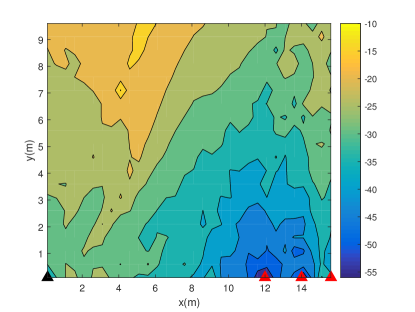
Figure 8: PEB (dB) of RIS localization using the Tx and Rxs.

Figure 9: Investigation of tracking accuracy over path 1 (a): For different values of the transmit power. (b): For different values of $T$ (c): Tracking error over the path. $\|\mathbf{v}[0]\|=10$m$/$s, $\|\mathbf{a}\|=2$m$/{\mathrm{s}}^{2}$.

Figure 10: Average of the CDFs of error over path 1 for different variances of initial localization error. $\|\mathbf{v}[0]\|=10$m$/$s, $\|\mathbf{a}\|=2$m$/{\rm s}^{2}$. The values of the average error over the path for $\sigma_{0}=0$, $\sigma_{0}=0.05$ and $\sigma_{0}=0.2$ are equal to $8.48\times 10^{-4}$, $4.38\times 10^{-2}$ and $0.18$, respectively.

To calculate this, let us define

$$\mbox{\boldmath{$\beta$}}= [\tau_{1,1},\alpha_{1,1},g_{1,1},f_{{}_{\mathrm{d},1,1}},\dots\tau_{1,N_{\mathrm{r}}},\alpha_{1,N_{\mathrm{r}}},g_{1,N_{\mathrm{r}}},f_{{}_{\mathrm{d},1,N_{\mathrm{r}}}},\dots$$

$$\tau_{K,1},\alpha_{K,1},g_{K,1},f_{{}_{\mathrm{d},K,1}},\dots,\tau_{K,N_{\mathrm{r}}},\alpha_{K,N_{\mathrm{r}}},g_{K,N_{\mathrm{r}}},f_{{}_{\mathrm{d},K,N_{\mathrm{r}}}}].$$

The $(i,j)^{\mathrm{th}}$ component of $\mathbf{I}_{\mbox{\boldmath{$\beta$}}}$, the information matrix of vector $\beta$, is equal to $\left[\mathbf{I}_{\mbox{\boldmath{$\beta$}}}\right]_{i,j}=\mathcal{R}\left\{\left[\frac{\partial\mathbf{f}}{\partial\beta_{i}}\right]^{H}\mathbf{Q}_{\mathbf{z}}\left[\frac{\partial\mathbf{f}}{\partial\beta_{j}}\right]\right\}$. For $k\in\mathcal{K}$, and $n_{\mathrm{r}}\in\mathcal{N}_{\mathrm{r}}$, the elements of the derivative of vector $\mathbf{f}$ with respect to $\beta_{i}$ for $i=4\gamma_{2}(k,N_{\mathrm{r}})+4n_{\mathrm{r}}-3$ are as

$$\!\!\!\!\left[\frac{\partial\mathbf{f}}{\partial\beta_{4\gamma_{2}(k,N_{\mathrm{r}})+4n_{\mathrm{r}}-3}}\right]_{\gamma_{1}(n,\bar{t},n_{\mathrm{r}})}=$$ (24)

$$\sqrt{E_{s}}g_{k,n_{\mathrm{r}}}(j2\pi(n-1)\Delta f)\sum\limits_{m=1}^{M}\left[\mbox{\boldmath{$\Phi$}}_{k}(\bar{t})\right]_{m,m}\mu(n,k,n_{\mathrm{r}},m).$$

Moreover, the elements of $\frac{\partial\mathbf{f}}{\partial\beta_{i}}$ for $i=4\gamma_{2}(k,N_{\mathrm{r}})+4n_{\mathrm{r}}-2$ are equal to

$$\left[\frac{\partial\mathbf{f}}{\partial\beta_{4\gamma_{2}(k,N_{\mathrm{r}})+4n_{\mathrm{r}}-2}}\right]_{\gamma_{1}(n,\bar{t},n_{\mathrm{r}})}=$$ (25)

$$j\frac{2\pi}{\lambda}d\sqrt{E_{s}}g_{k,n_{\mathrm{r}}}\sum\limits_{m=1}^{M}(m-1)\left[\mbox{\boldmath{$\Phi$}}_{k}(\bar{t})\right]_{m,m}\mu(n,k,n_{\mathrm{r}},m),$$

and for $i=4\gamma_{2}(k,N_{\mathrm{r}})+4n_{\mathrm{r}}-1$ and $i=4\gamma_{2}(k,N_{\mathrm{r}})+4n_{\mathrm{r}}$ are given by (26) and (27), respectively.

$$\left[\frac{\partial\mathbf{f}}{\partial\beta_{4\gamma_{2}(k,N_{\mathrm{r}})+4n_{\mathrm{r}}-1}}\right]_{\gamma_{1}(n,\bar{t},n_{\mathrm{r}})}\!\!\!\!\!\!\!\!\!\!\!\!\!\!\!\!\!\!\!\!=\sqrt{E_{s}}\sum\limits_{m=1}^{M}\!\!\left[\mbox{\boldmath{$\Phi$}}_{k}(\bar{t})\right]_{m,m}\mu(n,k,n_{\mathrm{r}},m),$$ (26)

$$\left[\frac{\partial\mathbf{f}}{\partial\beta_{4\gamma_{2}(k,N_{\mathrm{r}})+4n_{\mathrm{r}}}}\right]_{\gamma_{1}(n,\bar{t},n_{\mathrm{r}})}=$$ (27)

$$\sqrt{E_{s}}g_{k,n_{\mathrm{r}}}(j2\pi T_{\mathrm{d}}(\bar{t}-1))\sum\limits_{m=1}^{M}\left[\mbox{\boldmath{$\Phi$}}_{k}(\bar{t})\right]_{m,m}\mu(n,k,n_{\mathrm{r}},m).$$

The CRLBs of $\tau_{k,n_{\mathrm{r}}}$ and $\alpha_{k,n_{\mathrm{r}}}$ are respectively equal to $[\mathbf{J}_{\mbox{\boldmath{$\beta$}}}]_{4\gamma_{2}(k,N_{\mathrm{r}})+4n_{\mathrm{r}}-3,4\gamma_{2}(k,N_{\mathrm{r}})+4n_{\mathrm{r}}-3}$ and $[\mathbf{J}_{\mbox{\boldmath{$\beta$}}}]_{4\gamma_{2}(k,N_{\mathrm{r}})+4n_{\mathrm{r}}-2,4\gamma_{2}(k,N_{\mathrm{r}})+4n_{\mathrm{r}}-2}$ in which $\mathbf{J}_{\mbox{\boldmath{$\beta$}}}=\mathbf{I}_{\mbox{\boldmath{$\beta$}}}^{-1}$.

VI Simulation Results

In this Section, we provide the simulation results to demonstrate the performance of the proposed localization and tracking approaches. We consider a Tx located at $\mathbf{p}_{{}_{\rm t}}=[0,0]$ and three Rxs located at $\mathbf{p}_{{}_{\mathrm{r},1}}=[12,0]$, $\mathbf{p}_{{}_{\mathrm{r},2}}=[14,0]$ and $\mathbf{p}_{{}_{\mathrm{r},3}}=[16,0]$, respectively. In each simulation two RISs are considered such that the location of one of them is as explained in the caption of the figures, while the location of the other RIS is random and the results are averaged on this location. The other simulation settings are as shown in Table II. In the following, we present the simulations of the localization and tracking approaches, each in an individual subsection. For the localization performance we use the approach of [31] as a benchmark. To have a fair comparison, our proposed phase shift design approach is used for both the localization approaches and the number of the transmissions are the same.

TABLE II: Simulation parameters

Parameter	Value
Carrier Frequency ($f_{c}$)	$6$GHz
RIS element spacing ($d$)	$\lambda/4$
Total Transmit power ($NE_{s}$)	$30$dBm
Number of subcarriers ($N$)	$512$
Subcarrier bandwidth ($\Delta_{f}$)	$120$ kHz
$T$	$32$
$N_{T}$	$2$
FFT dimensions ($N_{f,\tau}$)	$8192$
FFT dimensions ($N_{f,f_{{}_{\mathrm{d}}}}$)	$1024$
The angle of orientation of the RIS ($\psi_{k,n_{\mathrm{r}}}$)	$\pi/6$
$N_{0}$	$-174\ \text{dBm/Hz}$

VI-A Localization Performance

In this Section, we investigate the performance of the proposed localization approach.

VI-A1 Effect of Number of Rxs

We explore the effect of the number of Rxs on the performance of the proposed localization approach as depicted in Fig. 3. In this figure, we compare the localization error of the systems with three, five, and nine Rxs in terms of $\Delta_{f}$, $N$ and total transmit power. As expected, we observe that increasing the number of Rxs enhances the localization accuracy. Obviously, this improvement is resulted by leveraging a larger set of measurements made available by larger number of Rxs.

VI-A2 Effect of Parameters $N_{T}$ and $T$

In Fig. 4, we verify the impact of the parameters $N_{T}$ and $T$ on the localization error of the proposed approach and PEB. In Fig. 4, we observe that increasing the number of transmissions by increasing $N_{T}$ reduces the error of the localization approach as well as the value of PEB. It is noticeable that increasing $N_{T}$ actually improves the accuracy of the estimation of $\alpha_{k}$ (see (11)). In Fig. 4, we notice that increasing $T$ also improves the accuracy of the localization approach and the PEB, which is due to the effect of increasing $T$ on the variance of the noise of the observation vector. However, we must note that enhancing the performance of the localization approach by increasing values of $N_{T}$ and $T$ will be at the cost of increasing the delay and power consumption for localization. Also, it is notable that the discrepancy between the PEB and the localization error stems from the fact that the CRLB does not consider the available resolution and cares more about the accuracy relying the assumption that the problem is resolvable. However, in the proposed localization approach we utilize the FFT method as a practical estimator for the ToA and the Doppler shift, which is constrained by the resolution of the FFT operation, which depends on the bandwidth.

VI-A3 Effect of Parameters $\Delta_{f}$, $N$ and Total Transmit Power

In Fig. 5, we investigate the effect of subcarrier bandwidth ($\Delta_{f}$), number of subcarriers ($N$) and total transmit power on the performance of the proposed localization approach and compare the results with [31]. In Fig. 5, we illustrate the localization error in terms of $\Delta_{f}$ for different values of $N$. We observe that increasing the subcarrier bandwidth, enhances the accuracy of both the localization approaches. Indeed, by increasing the value of $\Delta_{f}$ the accuracy of ToAs estimation is improved, leading to better localization results. Also, we can note that the proposed approach has significantly enhanced the localization accuracy in comparison with [31]. Specifically, in this case, our approach achieves the same localization accuracy, but at a half number of subcarriers. In Fig. 5, we plot the localization error in terms of $N$. We observe that increasing the number of subcarriers leads to a reduction in the localization error for both the proposed approaches. We can note that in the case of the proposed localization approach, increasing the number of subcarriers actually enhances the estimation of $\alpha_{k,n_{\mathrm{r}}}$ as well as the estimation of $\tau_{k,n_{\mathrm{r}}}$ (see (8) and Algorithm 1). In Fig.5, we depict the localization error in terms of total transmit power for different subcarrier bandwidths. We observe that as expected, increasing the transmit power reduces the error of both the localization approaches due to the improvement of the signal-to-noise ratio (SNR) of the received signals. Moreover, for a localization accuracy of $0.1$m, our proposed localization approach reduces the transmit power roughly by 20$\%$.

In Fig. 6, we investigate the effect of $\Delta_{f}$ and $N$ as the total bandwidth is fixed. We depict the localization error in terms of $\Delta_{f}$ and $N$, for different bandwidth values BW$=256\times 120$kHz and BW$=512\times 120$kHz. We observe that for both the localization approaches, there is a optimal value for $\Delta_{f}$ and $N$.

VI-A4 Effect of the Position of the RIS

To further investigate the performance of the proposed approach, in Fig. 7, we examine its performance in terms of the $x$-coordinate and $y$-coordinate of the RIS location. In Fig. 7, it is evident that as the distance between the RIS and the line between the Tx and Rx increases, the superiority of the proposed approach over [31] becomes more pronounced. Also, Fig. 7 shows the improvement of the accuracy by the proposed approach for different values of $x$. The behaviour of the curves in terms of $x$ and $y$ can be attributed to the PEB of the localization in various points of the region. In this regard, we plot the heat map of the PEB in Fig. 8. We observe that as the distance between the RIS and the line between the Tx and Rx increases, the PEB tends to increase. Moreover, the minimum PEB occurs near the Rxs, while near the Tx the error is higher.

Figure 11: Investigation of tracking accuracy, (a): Tracked paths. (b): Average CDF of the error of the proposed tracking and localization approach over the paths. For paths 1 and 2 $\|\mathbf{v}[0]\|=10$m$/$s, for paths 3 and 4 $\|\mathbf{v}[0]\|=20$m$/$s, and for all paths $\|\mathbf{a}\|=2$m$/{\mathrm{s}}^{2}$. The values of the average error of the tracking approach over the paths are equal to $0.14$, $0.26$, $0.16$ and $0.43$, respectively. Also, the values of the average error of the localization approach over the paths are equal to $0.21$, $0.32$, $0.42$ and $0.66$, respectively.

VI-B Tracking Performance

Now, we investigate the performance of the proposed tracking approach. In this regard, we examine the tracking of path 1 in Fig. 9. In Fig. 9 and Fig. 9, we plot the tracked path using different values of $T$ and transmit power, and also using the proposed localization approach. We observe that both increasing $T$ and the transmit power could improve the accuracy of the tracking approach. Also, comparing the tracking and localization approach we can observe that in most points the accuracy of the tracking approach is higher. Moreover, the benefit of the tracking approach compared to the localization is that in tracking the error at each point is less compared to the previous points. In Fig. 9, we illustrate the error of the tracking approach over path 1. We observe that as expected, for different values of $T$ and transmit power the tracking approach reduces the error of the localization over the time.

In Fig. 10, we investigate the effect of the initial localization error on the error of tracking over the path. In this Fig., we illustrate the average CDF of the error over the path for different values of standard deviation of the initial localization error and also obtain the average error over the path. We observe that as expected the accuracy of the tracking error is affected by the variance of the initial error, but for each variance the tracking error reduces the average error compared to the error of the initial point.

To further investigate the performance of the tracking approach, in Fig. 11, we examine the tracking approach for two different initial velocities, and also compare the accuracy of the tracking over each path with accuracy of the localization approach. The initial velocity of the RIS on paths 1 and 2 is $10{\rm m/s}$, while its initial velocity on paths 3 and 4 is $20{\rm m/s}$. In Fig. 11, we observe that in all the cases the tracking approach compensates the initial error along the path. In Fig. 11, we compare the average CDFs of the error of the tracking and the localization approaches over the paths. We observe that on average over each path the tracking approach could increase the probability of having less error, for different values of $e$, compared to the localization approach.

VII Conclusion

In this paper, we investigated the problem of tracking RISs employing a single antenna transmitter and multiple single antenna receivers. In this regard, we proposed a phase shift design approach to eliminate the effects of scatters and extract the signal passed through each RIS. Then, we proposed a localization approach to estimate the initial location of the RISs. The simulation results demonstrate that this approach outperforms the previously proposed ToA-based approach. Finally, based on the EKF approach we proposed a tracking algorithm. The simulation results confirm the accuracy of the proposed tracking approach.

$$[{\bf H}_{k}[n|n-1]]_{N_{\mathrm{r}}+n_{\mathrm{r}},1}=\cos\psi_{k,n_{\mathrm{r}}}\Big{(}\frac{\left(p_{k,1}[n|n-1]-p_{{\rm t},1}\right)}{\left|p_{k,1}[n|n-1]-p_{{\rm t},1}\right|\left\|\mathbf{p}_{{}_{k}}[n|n-1]-\mathbf{p}_{{}_{\rm t}}\right\|}-\frac{\left(p_{k,1}[n|n-1]-p_{{\rm t},1}\right)\left|p_{k,1}[n|n-1]-p_{{\rm t},1}\right|}{\left\|\mathbf{p}_{{}_{k}}[n|n-1]-\mathbf{p}_{{}_{\rm t}}\right\|^{3}}\vspace{1mm}$$

$$-\frac{\left(p_{k,1}[n|n-1]-p_{{\rm r},n_{r},1}\right)}{\left|p_{k,1}[n|n-1]-p_{{\rm r},n_{r},1}\right|\left\|\mathbf{p}_{{}_{k}}[n|n-1]-\mathbf{p}_{{}_{\mathrm{r},n_{r}}}\right\|}+\frac{\left(p_{k,1}[n|n-1]-p_{{\rm r},n_{r},1}\right)\left|p_{k,1}[n|n-1]-p_{{\rm r},n_{r},1}\right|}{\left\|\mathbf{p}_{{}_{k}}[n|n-1]-\mathbf{p}_{{}_{\mathrm{r},n_{r}}}\right\|^{3}}\Big{)}+$$

$$\sin\psi_{k,n_{\mathrm{r}}}\Big{(}-\frac{\left|p_{k,2}[n|n-1]-p_{{\rm t},2}\right|\left(p_{k,1}[n|n-1]-p_{{\rm t},1}\right)}{\left\|\mathbf{p}_{{}_{k}}[n|n-1]-\mathbf{p}_{{}_{\rm t}}\right\|^{3}}-\frac{\left|p_{k,2}[n|n-1]-p_{{\rm r},n_{r},2}\right|\left(p_{k,1}[n|n-1]-p_{{\rm r},n_{r},1}\right)}{\left\|\mathbf{p}_{{}_{k}}[n|n-1]-\mathbf{p}_{{}_{\mathrm{r},n_{r}}}\right\|^{3}}\Big{)}.$$ (35)

$$[{\bf H}_{k}[n|n-1]]_{N_{\mathrm{r}}+n_{\mathrm{r}},2}=\cos\psi_{k,n_{\mathrm{r}}}\Big{(}-\frac{\left|p_{k,1}[n|n-1]-p_{{\rm t},1}\right|\left(p_{k,2}[n|n-1]-p_{{\rm t},2}\right)}{\left\|\mathbf{p}_{{}_{k}}[n|n-1]-\mathbf{p}_{{}_{\rm t}}\right\|^{3}}+$$

$$\frac{\left|p_{k,1}[n|n-1]-p_{{\rm r},n_{r},1}\right|\left(p_{k,2}[n|n-1]-p_{{\rm r},n_{r},2}\right)}{\left\|\mathbf{p}_{{}_{k}}[n|n-1]-\mathbf{p}_{{}_{\mathrm{r},n_{r}}}\right\|^{3}}\Big{)}+\sin\psi_{k,n_{\mathrm{r}}}\Big{(}\frac{\left(p_{k,2}[n|n-1]-p_{{\rm t},2}\right)}{\left|p_{k,2}[n|n-1]-p_{{\rm t},2}\right|\left\|\mathbf{p}_{{}_{k}}[n|n-1]-\mathbf{p}_{{}_{\rm t}}\right\|}$$

$$-\frac{\left(p_{k,2}[n|n-1]-p_{{\rm t},2}\right)\left|p_{k,2}[n|n-1]-p_{{\rm t},2}\right|}{\left\|\mathbf{p}_{{}_{k}}[n|n-1]-\mathbf{p}_{{}_{\rm t}}\right\|^{3}}\vspace{1mm}+\frac{\left(p_{k,2}[n|n-1]-p_{{\rm r},n_{r},2}\right)}{\left|p_{k,2}[n|n-1]-p_{{\rm r},n_{r},2}\right|\left\|\mathbf{p}_{{}_{k}}[n|n-1]-\mathbf{p}_{{}_{\mathrm{r},n_{r}}}\right\|}$$

$$-\frac{\left(p_{k,2}[n|n-1]-p_{{\rm r},n_{r},2}\right)\left|p_{k,2}[n|n-1]-p_{{\rm r},n_{r},2}\right|}{\left\|\mathbf{p}_{{}_{k}}[n|n-1]-\mathbf{p}_{{}_{\mathrm{r},n_{r}}}\right\|^{3}}\Big{)}.$$ (36)

Appendix A

In this appendix, we derive the partial derivatives of $\tau_{k,n_{\mathrm{r}}}$ and $\alpha_{k,n_{\mathrm{r}}}$, and using them obtain the elements of matrix ${\bf H}_{k}[n|n-1]$. The partial derivative of $\tau_{k,n_{\mathrm{r}}}$ with respect to $p_{k,i}$ for $i=1,2$ is equal to

$$\frac{\partial\tau_{k,n_{\mathrm{r}}}}{\partial p_{k,i}}=\frac{p_{k,i}-p_{{\rm t},i}}{c\left\|\mathbf{p}_{{}_{k}}-\mathbf{p}_{{}_{\rm t}}\right\|}+\frac{p_{k,i}-p_{{\rm r},n_{\mathrm{r}},i}}{c\left\|\mathbf{p}_{{}_{k}}-\mathbf{p}_{{}_{\mathrm{r},n_{r}}}\right\|},\ i=1,2,$$ (28)

and the partial derivatives of $\alpha_{k,n_{\mathrm{r}}}$ with respect to $p_{k,1}$ and $p_{k,2}$ are respectively given as

$$\frac{\partial\alpha_{k,n_{\mathrm{r}}}}{\partial p_{k,1}}=\cos\psi_{k,n_{\mathrm{r}}}\left(\frac{\left(p_{k,1}-p_{{\rm t},1}\right)}{\left|p_{k,1}-p_{{\rm t},1}\right|\left\|\mathbf{p}_{{}_{k}}-\mathbf{p}_{{}_{\rm t}}\right\|}\right.$$

$$-\frac{\left(p_{k,1}-p_{{\rm t},1}\right)\left|p_{k,1}-p_{{\rm t},1}\right|}{\left\|\mathbf{p}_{{}_{k}}-\mathbf{p}_{{}_{\rm t}}\right\|^{3}}-\frac{\left(p_{k,1}-p_{{\rm r},n_{r},1}\right)}{\left|p_{k,1}-p_{{\rm r},n_{r},1}\right|\left\|\mathbf{p}_{{}_{k}}-\mathbf{p}_{{}_{\mathrm{r},n_{r}}}\right\|}+$$

$$\left.\frac{\left(p_{k,1}-p_{{\rm r},n_{r},1}\right)\left|p_{k,1}-p_{{\rm r},n_{r},1}\right|}{\left\|\mathbf{p}_{{}_{k}}-\mathbf{p}_{{}_{\mathrm{r},n_{r}}}\right\|^{3}}\right)+$$

$$\sin\psi_{k,n_{\mathrm{r}}}\left(\frac{\left(p_{k,2}-p_{{\rm t},2}\right)}{\left|p_{k,2}-p_{{\rm t},2}\right|\left\|\mathbf{p}_{{}_{k}}-\mathbf{p}_{{}_{\rm t}}\right\|}-\right.$$

$$\frac{\left(p_{k,2}-p_{{\rm t},2}\right)\left|p_{k,2}-p_{{\rm t},2}\right|}{\left\|\mathbf{p}_{{}_{k}}-\mathbf{p}_{{}_{\rm t}}\right\|^{3}}+\frac{\left(p_{k,2}-p_{{\rm r},n_{r},2}\right)}{\left|p_{k,2}-p_{{\rm r},n_{r},2}\right|\left\|\mathbf{p}_{{}_{k}}-\mathbf{p}_{{}_{\mathrm{r},n_{r}}}\right\|}$$

$$\left.-\frac{\left(p_{k,2}-p_{{\rm r},n_{r},2}\right)\left|p_{k,2}-p_{{\rm r},n_{r},2}\right|}{\left\|\mathbf{p}_{{}_{k}}-\mathbf{p}_{{}_{\mathrm{r},n_{r}}}\right\|^{3}}\right),$$ (29)

and

$$\frac{\partial\alpha_{k,n_{\mathrm{r}}}}{\partial p_{k,2}}=-\frac{\left|p_{k,2}-p_{{\rm t},2}\right|\left(p_{k,1}-p_{{\rm t},1}\right)}{\left\|\mathbf{p}_{{}_{k}}-\mathbf{p}_{{}_{\rm t}}\right\|^{3}}$$

$$-\frac{\left|p_{k,2}-p_{{\rm r},n_{r},2}\right|\left(p_{k,1}-p_{{\rm r},n_{r},1}\right)}{\left\|\mathbf{p}_{{}_{k}}-\mathbf{p}_{{}_{\mathrm{r},n_{r}}}\right\|^{3}}.$$ (30)

Thus, considering (19), the elements $(n_{\mathrm{r}},i)$ of ${\bf H}_{k}[n|n-1]$ for $n_{\mathrm{r}}\in\mathcal{N}_{\mathrm{r}}$ and $i=1,\dots,4$ would be as follows

$$[{\bf H}_{k}[n|n-1]]_{n_{\mathrm{r}},1}=\frac{p_{k,1}[n|n-1]-p_{{\rm t},1}}{\left\|\mathbf{p}_{{}_{k}}[n|n-1]-\mathbf{p}_{{}_{\rm t}}\right\|}$$ (31)

$$+\frac{p_{k,1}[n|n-1]-p_{{\rm r},n_{r},1}}{\left\|\mathbf{p}_{{}_{k}}[n|n-1]-\mathbf{p}_{{}_{\mathrm{r},n_{r}}}\right\|},$$

$$[{\bf H}_{k}[n|n-1]]_{n_{\mathrm{r}},2}=\frac{p_{k,2}[n|n-1]-p_{{\rm t},2}}{\left\|\mathbf{p}_{{}_{k}}[n|n-1]-\mathbf{p}_{{}_{\rm t}}\right\|}$$ (32)

$$+\frac{p_{k,2}[n|n-1]-p_{{\rm r},n_{r},2}}{\left\|\mathbf{p}_{{}_{k}}[n|n-1]-\mathbf{p}_{{}_{\mathrm{r},n_{r}}}\right\|},$$

$$[{\bf H}_{k}[n|n-1]]_{n_{\mathrm{r}},3}=T_{s}\frac{p_{k,1}[n|n-1]-p_{{\rm t},1}}{\left\|\mathbf{p}_{{}_{k}}[n|n-1]-\mathbf{p}_{{}_{\rm t}}\right\|}$$ (33)

$$+T_{s}\frac{p_{k,1}[n|n-1]-p_{{\rm r},n_{r},1}}{\left\|\mathbf{p}_{{}_{k}}[n|n-1]-\mathbf{p}_{{}_{\mathrm{r},n_{r}}}\right\|},$$

$$[{\bf H}_{k}[n|n-1]]_{n_{\mathrm{r}},4}=T_{s}\frac{p_{k,2}[n|n-1]-p_{{\rm t},2}}{\left\|\mathbf{p}_{{}_{k}}[n|n-1]-\mathbf{p}_{{}_{\rm t}}\right\|}$$ (34)

$$+T_{s}\frac{p_{k,2}[n|n-1]-p_{{\rm r},n_{r},2}}{\left\|\mathbf{p}_{{}_{k}}[n|n-1]-\mathbf{p}_{{}_{\mathrm{r},n_{r}}}\right\|}.$$

Additionally, the elements $(n_{\mathrm{r}}+N_{\mathrm{r}},i)$ of ${\bf H}_{k}[n|n-1]$ for $n_{\mathrm{r}}\in\mathcal{N}_{\mathrm{r}}$ and $i=1,\dots,4$ are as (35), (36), (37) and (38).

$$[{\bf H}_{k}[n|n-1]]_{N_{\mathrm{r}}+n_{\mathrm{r}},3}=T_{s}[{\bf H}_{k}[n|n-1]]_{N_{\mathrm{r}}+n_{\mathrm{r}},1}.$$ (37)

$$[{\bf H}_{k}[n|n-1]]_{N_{\mathrm{r}}+n_{\mathrm{r}},4}=T_{s}[{\bf H}_{k}[n|n-1]]_{N_{\mathrm{r}}+n_{\mathrm{r}},2}.$$ (38)

Somayeh Aghashahi (S’16) received the B.Sc. degree in pure mathematics from Shahid Bahonar University of Kerman, Kerman, Iran, in 2013, and received the M.Sc. degree in communication systems engineering from Yazd Unversity, Yazd, Iran, in 2018, where she is currently pursuing the Ph.D degree in communication systems engineering. Her research interests include wireless communication and statistical signal processing with a particular emphasis on MIMO communications, RIS and reconfigurable antennas assisted communication and localization.

Zolfa Zeinalpour-Yazdi received the B.S., M.S., and Ph.D. degrees in electrical engineering from the Sharif University of Technology, Tehran, Iran, in 2002, 2004, and 2010, respectively. She was a Visiting Researcher with ftw. Telecommunication Research Center, Vienna, Austria, in 2006. She joined Yazd University in 2010, where she is currently an Associate Professor with the Department of Electrical Engineering. Her research interest includes the broad area of wireless communications and currently, she is working towards next generation of wireless networks and mathematical treatment of the problems in these areas with a particular emphasis on stochastic analysis of heterogeneous networks, vehicular communications, RIS-empowered transmissions and also interference management and caching strategy in these networks.

Aliakbar Tadaion (S’ 05-M’ 07-SM’ 13) was born in Iran in 1976. He received the B.Sc. degree in electronics, the M.Sc. and Ph.D. degrees in communication systems all from Sharif University of Technology, Tehran, Iran, in 1998, 2000 and 2006, respectively. From August 2004 to June 2005, he was with the Department of Electrical and Computer Engineering, Queen’s University, Kingston, ON, Canada, as the visiting researcher. He joined the department of electrical Engineering, Yazd University, Yazd, Iran in Sep. 2005, where he is now a Professor. He is also the founder and director of Cell Lab. Now he is a senior member of the Institute of Electrical and Electronics Engineers (IEEE) and also since Jan. 2013, he has been a member of the excom committee of IEEE Iran Section and the newsletter editor of the Iran Section. He has been the technical program committee member of some conferences, such as WOSSPA 2011, IWCIT 2013-2024 and has served as an organizing committee member of some conferences such as ISCC 2012.

Mahdi Boloursaz Mashhadi (S’15-M’19-SM’23) is a Lecturer at the 5G/6G Innovation Centre (5G/6GIC) at the Institute for Communication Systems (ICS), University of Surrey (UoS), and a Surrey AI fellow. His research is focused at the intersection of AI/ML with wireless communication, learning and communication co-design, generative AI for telecommunications, and collaborative machine learning. He received B.S., M.S., and Ph.D. degrees in mobile telecommunications from the Sharif University of Technology (SUT), Tehran, Iran. He has more than 40 peer reviewed publications and patents in the areas of wireless communications, machine learning, and signal processing. He is a PI/Co-PI for various government and industry funded projects including the UKTIN/DSIT 12M£ national project TUDOR. He received the Best Paper Award from the IEEE EWDTS conference, and the Exemplary Reviewer Award from the IEEE ComSoc in 2021 and 2022. He served as a panel judge for the International Telecommunication Union (ITU) on the “AI/ML in 5G” challenge 2021-2022. He is an associate editor for the Springer Nature Wireless Personal Communications Journal.

Ahmed Elzanaty (S’13-M’18-SM’22) received his PhD degree (cum laude) in electronics, telecommunications, and information technology from the University of Bologna, Italy, in 2018. Currently, he is a Lecturer (Assistant Professor) with the Institute for Communication Systems, University of Surrey, U.K. Before that, he was a Postdoctoral Fellow at the King Abdullah University of Science and Technology (KAUST), Saudi Arabia. He has participated in several national and European projects, such as TUDOR, CHEDDAR, and EuroCPS. His research interests include the design and performance analysis of wireless communications and localization systems.

References

• [1] F. Liu, Y. Cui, C. Masouros, J. Xu, T. X. Han, Y. C. Eldar, and S. Buzzi, “Integrated sensing and communications: Toward dual-functional wireless networks for 6G and beyond,” IEEE journal on selected areas in commun., vol. 40, no. 6, pp. 1728–1767, 2022.
• [2] Z. Wei, H. Qu, Y. Wang, X. Yuan, H. Wu, Y. Du, K. Han, N. Zhang, and Z. Feng, “Integrated sensing and communication signals towards 5G-A and 6G: A survey,” IEEE Internet of Things Journal, 2023.
• [3] C. De Lima, D. Belot, R. Berkvens, A. Bourdoux, D. Dardari, M. Guillaud, M. Isomursu, E.-S. Lohan, Y. Miao, A. N. Barreto, M. R. K. Aziz, J. Saloranta, T. Sanguanpuak, H. Sarieddeen, G. Seco-Granados, J. Suutala, T. Svensson, M. Valkama, B. Van Liempd, and H. Wymeersch, “Convergent communication, sensing and localization in 6G systems: An overview of technologies, opportunities and challenges,” IEEE Access, vol. 9, pp. 26 902–26 925, 2021.
• [4] A. Adhikary, M. S. Munir, A. D. Raha, Y. Qiao, Z. Han, and C. S. Hong, “Integrated sensing, localization, and communication in holographic MIMO-enabled wireless network: A deep learning approach,” IEEE trans. on Network and Service Management, pp. 1–1, 2023.
• [5] T. Wu, C. Pan, Y. Pan, S. Hong, H. Ren, M. Elkashlan, F. Shu, and J. Wang, “Joint angle estimation error analysis and 3-D positioning algorithm design for mmwave positioning system,” IEEE Internet of Things Journal, vol. 11, no. 2, pp. 2181–2197, 2024.
• [6] J. A. del Peral-Rosado, R. Raulefs, J. A. López-Salcedo, and G. Seco-Granados, “Survey of cellular mobile radio localization methods: From 1G to 5G,” IEEE commun. Surveys & Tutorials, vol. 20, no. 2, pp. 1124–1148, 2017.
• [7] A. Elzanaty, A. Guerra, F. Guidi, D. Dardari, and M.-S. Alouini, “Towards 6G holographic localization: Enabling technologies and perspectives,” IEEE Internet of Things Magazine, 2023.
• [8] Q. Wu and R. Zhang, “Towards smart and reconfigurable environment: Intelligent reflecting surface aided wireless network,” IEEE Commun. Mag., vol. 58, no. 1, pp. 106–112, Nov. 2019.
• [9] Y. Liu, X. Liu, X. Mu, T. Hou, J. Xu, M. Di Renzo, and N. Al-Dhahir, “Reconfigurable intelligent surfaces: Principles and opportunities,” IEEE commun. surveys & tutorials, vol. 23, no. 3, pp. 1546–1577, 2021.
• [10] S. Aghashahi, A. Tadaion, Z. Zeinalpour-Yazdi, M. B. Mashhadi, and A. Elzanaty, “EMF-aware energy efficient MU-SIMO systems with multiple RISs,” IEEE trans. on Vehicular Technology, pp. 1–6, 2023.
• [11] S. Aghashahi, Z. Zeinalpour-Yazdi, A. Tadaion, M. B. Mashhadi, and A. Elzanaty, “MU-massive MIMO with multiple RISs: SINR maximization and asymptotic analysis,” IEEE Wireless commun. Letters, vol. 12, no. 6, pp. 997–1001, 2023.
• [12] H. Wymeersch, J. He, B. Denis, A. Clemente, and M. Juntti, “Radio localization and mapping with reconfigurable intelligent surfaces: Challenges, opportunities, and research directions,” IEEE Vehicular Technology Magazine, vol. 15, no. 4, pp. 52–61, Dec. 2020.
• [13] K. Keykhosravi, B. Denis, G. C. Alexandropoulos, Z. S. He, A. Albanese, V. Sciancalepore, and H. Wymeersch, “Leveraging RIS-enabled smart signal propagation for solving infeasible localization problems: Scenarios, key research directions, and open challenges,” IEEE Vehicular Technology Magazine, vol. 18, no. 2, pp. 20–28, 2023.
• [14] T. Ma, Y. Xiao, X. Lei, W. Xiong, and Y. Ding, “Indoor localization with reconfigurable intelligent surface,” IEEE commun. Letters, vol. 25, no. 1, pp. 161–165, 2021.
• [15] T. Wu, C. Pan, Y. Pan, H. Ren, M. Elkashlan, and C.-X. Wang, “Fingerprint-based mmwave positioning system aided by reconfigurable intelligent surface,” IEEE Wireless Commun. Letters, vol. 12, no. 8, pp. 1379–1383, 2023.
• [16] T. Wu, C. Pan, K. Zhi, H. Ren, M. Elkashlan, C.-X. Wang, R. Schober, and X. You, “Exploit high-dimensional ris information to localization: What is the impact of faulty element?” IEEE Journal on Selected Areas in Communications, pp. 1–1, 2024.
• [17] T. Wu, C. Pan, K. Zhi, H. Ren, M. Elkashlan, J. Wang, and C. Yuen, “Employing high-dimensional RIS information for RIS-aided localization systems,” IEEE Commun. Letters, 2024.
• [18] A. Elzanaty, A. Guerra, F. Guidi, and M.-S. Alouini, “Reconfigurable intelligent surfaces for localization: Position and orientation error bounds,” IEEE trans. on Signal Processing, vol. 69, pp. 5386–5402, 2021.
• [19] O. Rinchi, A. Elzanaty, and M.-S. Alouini, “Compressive near-field localization for multipath RIS-aided environments,” IEEE commun. Letters, vol. 26, no. 6, pp. 1268–1272, 2022.
• [20] W. Wang and W. Zhang, “Joint beam training and positioning for intelligent reflecting surfaces assisted millimeter wave communications,” IEEE trans. on Wireless commun., vol. 20, no. 10, pp. 6282–6297, 2021.
• [21] K. Keykhosravi, M. F. Keskin, G. Seco-Granados, and H. Wymeersch, “SISO RIS-enabled joint 3D downlink localization and synchronization,” in ICC 2021 - IEEE International Conference on commun., 2021, pp. 1–6.
• [22] D. Dardari, N. Decarli, A. Guerra, and F. Guidi, “LOS/NLOS near-field localization with a large reconfigurable intelligent surface,” IEEE trans. on Wireless commun., 2021.
• [23] M. Luan, B. Wang, Y. Zhao, Z. Feng, and F. Hu, “Phase design and near-field target localization for RIS-assisted regional localization system,” IEEE trans. on Vehicular Technology, vol. 71, no. 2, pp. 1766–1777, 2022.
• [24] H. Zhang, H. Zhang, B. Di, K. Bian, Z. Han, and L. Song, “Towards ubiquitous positioning by leveraging reconfigurable intelligent surface,” IEEE commun. Letters, vol. 25, no. 1, pp. 284–288, 2020.
• [25] K. Keykhosravi, G. Seco-Granados, G. C. Alexandropoulos, and H. Wymeersch, “RIS-enabled self-localization: Leveraging controllable reflections with zero access points,” in ICC 2022-IEEE International Conference on Communications.   IEEE, 2022, pp. 2852–2857.
• [26] H. Kim, H. Chen, M. F. Keskin, Y. Ge, K. Keykhosravi, G. C. Alexandropoulos, S. Kim, and H. Wymeersch, “RIS-enabled and access-point-free simultaneous radio localization and mapping,” IEEE trans. on Wireless commun., pp. 1–1, 2023.
• [27] H. Chen, P. Zheng, M. F. Keskin, T. Al-Naffouri, and H. Wymeersch, “Multi-RIS-enabled 3D sidelink positioning,” IEEE Trans. on Wireless Commun., 2024.
• [28] M. Ammous, H. Chen, H. Wymeersch, and S. Valaee, “Zero access points 3D cooperative positioning via RIS and sidelink communications,” arXiv preprint arXiv:2305.08287, 2023.
• [29] M. Ammous and S. Valaee, “Positioning and tracking using reconfigurable intelligent surfaces and extended Kalman filter,” in 2022 IEEE 95th Vehicular Technology Conference: (VTC2022-Spring), 2022, pp. 1–6.
• [30] Y. Chen, Y. Wang, X. Guo, Z. Han, and P. Zhang, “Location tracking for reconfigurable intelligent surfaces aided vehicle platoons: Diverse sparsities inspired approaches,” IEEE Journal on Selected Areas in commun., pp. 1–1, 2023.
• [31] K. Keykhosravi, M. F. Keskin, S. Dwivedi, G. Seco-Granados, and H. Wymeersch, “Semi-passive 3D positioning of multiple RIS-enabled users,” IEEE trans. on Vehicular Technology, vol. 70, no. 10, pp. 11 073–11 077, 2021.
• [32] R. Ghazalian, K. Keykhosravi, H. Chen, H. Wymeersch, and R. Jäntti, “Bi-static sensing for near-field RIS localization,” in GLOBECOM 2022-2022 IEEE Global commun. Conference.   IEEE, 2022, pp. 6457–6462.
• [33] Y. Lu, H. Chen, J. Talvitie, H. Wymeersch, and M. Valkama, “Joint RIS calibration and multi-user positioning,” in 2022 IEEE 96th Vehicular Technology Conference (VTC2022-Fall).   IEEE, 2022, pp. 1–6.
• [34] P. Zheng, H. Chen, T. Ballal, M. Valkama, H. Wymeersch, and T. Y. Al-Naffouri, “JrCUP: Joint RIS calibration and user positioning for 6G wireless systems,” IEEE Trans. on Wireless Commun., 2023.
• [35] R. Ghazalian, H. Chen, G. C. Alexandropoulos, G. Seco-Granados, H. Wymeersch, and R. Jäntti, “Joint user localization and location calibration of a hybrid reconfigurable intelligent surface,” IEEE Trans. on Vehicular Technology, 2023.
• [36] T. Wu, C. Pan, Y. Pan, H. Ren, M. Elkashlan, and C.-X. Wang, “Fingerprint based mmwave positioning system aided by reconfigurable intelligent surface,” IEEE Wireless commun. Letters, pp. 1–1, 2023.
• [37] H. Chen, M. F. Keskin, A. Sakhnini, N. Decarli, S. Pollin, D. Dardari, and H. Wymeersch, “6g localization and sensing in the near field: Features, opportunities, and challenges,” IEEE Wireless Commun., 2024.
• [38] A. Fascista, M. F. Keskin, A. Coluccia, H. Wymeersch, and G. Seco-Granados, “RIS-aided joint localization and synchronization with a single-antenna receiver: Beamforming design and low-complexity estimation,” IEEE Journal of Selected Topics in Signal Processing, vol. 16, no. 5, pp. 1141–1156, 2022.
• [39] J. C. B. Garcia, A. Sibille, and M. Kamoun, “Reconfigurable intelligent surfaces: Bridging the gap between scattering and reflection,” IEEE Journal on Selected Areas in Commun., vol. 38, no. 11, pp. 2538–2547, 2020.
• [40] C. Zhang, W. Yi, Y. Liu, K. Yang, and Z. Ding, “Reconfigurable intelligent surfaces aided multi-cell NOMA networks: A stochastic geometry model,” IEEE Trans. on Commun., vol. 70, no. 2, pp. 951–966, 2021.
• [41] S. M. Kay, Fundamentals of statistical signal processing: estimation theory.   Prentice-Hall, Inc., 1993.