Gradient Mittag-Leffler and strong stabilizability
of time fractional diffusion processes

Abstract

This paper deals with the gradient stability and the gradient stabilizability of Caputo time fractional diffusion linear systems. First, we give sufficient conditions that allow the gradient Mittag-Leffler and strong stability, where we use a direct method based essentially on the spectral properties of the system dynamic. Moreover, we consider a class of linear and distributed feedback controls that Mittag-Leffler and strongly stabilize the state gradient. The proposed results lead to an algorithm that allows us to gradient stabilize the state of the fractional systems under consideration. Finally, we illustrate the effectiveness of the developed algorithm by a numerical example and simulations.

Keywords: decomposition approach, fractional diffusion systems, gradient stabilization, gradient stability, partial differential equations, distributed controls.

2020 Mathematics Subject Classification: 26A33, 35R11, 93C05, 93D15, 93D20.

1 Introduction

Fractional systems with Caputo derivative have gained significant attention in various fields, due to their physical meaning and wide applications, such as in epidemics [20, 22], porous and fractured media [17], population dynamics [2], etc. The class of fractional diffusion systems (FDSs) has been especially widely investigated in chemistry, physics (particle diffusion), biology, economics (diffusion of price values) and sociology (diffusion of people). Indeed, based on the continuous-time random walks theory, it is worth noting that FDSs can be used to efficiently describe anomalous diffusion processes with a highly heterogeneous aquifer, and offer better performance than using conventional diffusion systems [1]. For example, FDSs may modelize the relaxation phenomena in complex viscoelastic materials [10], the movement of plasma under high temperature and high pressure, and the power law decay of prime number distributions [3].

Stability is among the most extensively studied concepts in control theory since an unstable dynamical system is of no interest as it can explode anywhere and at any instant. It signifies that the system remains in a constant state unless affected by an external action and returns to its equilibrium state when the external action is detached. Also one of the challenging problems related to the stability analysis is stabilizability, which means that if a dynamical system is not stable by itself, then the question arises whether it may be stabilized by selecting suitable controller inputs.

In recent years, the analysis of the stability, stabilizability, and related problems of FDSs have been tackled in many works: see, e.g., [6, 9, 12, 23, 24]. For instance, in [23, 24] the authors consider different degrees of the state stability and stabilization: the strong and the exponential ones of fractional distributed systems involving both Caputo and Riemann–Liouville time derivatives of order $q\in(0,1]$. Furthermore, the decomposition approach is applied to conceive the state stabilizing feedback law. Moreover, in [9], the authors investigate the regional stabilization concept, where they present some results about the regional Mittag-Leffler and asymptotic stabilization of FDSs on a sub-region of the geometrical domain, while in [12], the boundary controller design and stability analysis for a time-space fractional diffusion equation are presented. Among other interesting concepts concerning the control theory of fractional diffusion systems one can find the gradient controllability [8] and gradient observability [7] in a sub-region of the geometrical domain of the Caputo and Riemann–Liouville time FDSs.

After analyzing the existing literature, it is evident that the gradient stability and stabilizability of FDSs are still untreated subjects in the literature and this fact is the motivation of the present work. Thus, the purpose of this paper is to derive some sufficient conditions that allow the gradient stability of Caputo fractional time systems of order $q\in(0,1]$ and also to design a control law that ensures the gradient stabilization of a class of fractional diffusion systems, defined on a bounded and connected subset $\Omega\subset\mathbb{R}^{n}$, $n=1,2,3,\ldots$ (with smooth boundary $\partial\Omega$) and described by

$$\left\{\begin{array}[]{ll}{}^{C}D_{t}^{q}y(x,t)=Ay(x,t)+Lv(x,t),&t\in]0,+\infty[,\\ y(\eta,t)=0,&\eta\in\partial\Omega,t\in]0,+\infty[,\\ y(x,0)=y_{0}(x),&y_{0}\in Y,\end{array}\right.$$ (1)

where the state space is $Y=H^{1}(\Omega)$, the operator $A:D(A)\subset Y\longrightarrow Y$ is linear and generates a $C_{0}$-semi-group $(T(t))_{t\geq 0}$ on $Y$ [5], $-A$ is a uniformly elliptic operator and $L$ is a linear bounded operator from $V_{ad}$ (the space of controls) into $Y$ with $v(t)$ a scalar input. Let ${}^{C}D_{t}^{q}$ be the left-sided Caputo fractional derivative [15] of order $q\in(0,1]$ with respect to time $t$, defined by

$${}^{C}D_{t}^{q}y(x,t)=\dfrac{1}{\Gamma(1-q)}\int_{0}^{t}(t-s)^{-q}\dfrac{d}{ds}y(x,s)\,\mathrm{d}s.$$

Moreover, we consider the gradient operator $\nabla$, which is defined by

$$\begin{array}[]{llcll}\nabla&:&Y&\mapsto&(L^{2}(\Omega))^{n}\\ &&y&\mapsto&\nabla y:=\left(\dfrac{\partial y}{\partial x_{1}},\dfrac{\partial y}{\partial x_{2}},\ldots,\dfrac{\partial y}{\partial x_{n}}\right).\end{array}$$

In particular, when $q=1$, the gradient stabilizability of the system (1) reduces to the gradient stabilizability of a classical integer order diffusion system, which is investigated in [21, 25]. It is worthy to mention that there are various applications of the gradient modeling. For instance, it is the exchange of the energy problem between a casting plasma on a plane target, which is perpendicular to the direction of the flow sub-diffusion process from measurements carried out by internal thermocouples. Another example is the concentration regulation of a substrate at the upper bottom of a biological reactor sub-diffusion process, which is observed between two levels [7]. For a richer background on gradient models, we refer the reader to [4, 14]. Indeed, gradient stabilization plays an important role in enhancing the reliability and efficiency of different engineering and physical systems. In particular, gradient stabilization methods can be applied to various real-world problems. For instance, in aerospace engineering, when simulating airflow around aircraft, the presence of shock waves can introduce instabilities. Gradient stabilization helps to maintain numerical stability, enabling engineers to accurately predict lift and drag forces, which are vital for optimizing aircraft performance and fuel efficiency. Moreover, in structural engineering, maintaining the stability of structures under varying loads is crucial. Therefore, gradient stabilization methods can be applied to optimize the design of beams, bridges, and buildings [16].

The remainder contents of this paper are structured as follows. In Section 2, we examine the state gradient Mittag-Leffler and strong stability. In Section 3, under sufficient conditions, we present a class of distributed feedback controls that ensure the state gradient Mittag-Leffler and strong stabilization of fractional time diffusion systems using two approaches: the first one concerns the decomposition method and the second one is based on the completely monotonic property of Mittag-Leffler functions and also on the spectrum properties of the operator $A$. In Section 4, we illustrate our theoretical results by a numerical example and simulations. In the last section, Section 5, we give a conclusion and some possible directions of future research.

2 Gradient stability

Throughout this paper, the spaces $Y$ and $L^{2}(\Omega)^{n}$ are endowed with the usual inner products $\langle\cdot,\cdot\rangle$ and $<\cdot,\cdot>_{n}$ and the associated norms $\Arrowvert\cdot\Arrowvert$ and $\Arrowvert\cdot\Arrowvert_{L^{2}(\Omega)^{n}}$, respectively. By $\nabla^{*}$ we denote the adjoint operator of the gradient operator $\nabla$. Moreover, to avoid confusion, we shall sometimes denote $y(\cdot,t):=y(t)$.

In this section, we explore some sufficient conditions for the gradient Mittag-Leffler and strong stability of the fractional linear diffusion system (1) with the control operator $L=0$.

We first give the following gradient stability definitions.

Definition 1.

Let $y_{0}\in Y$. The system (1) is said to be

• Gradient Mittag-Leffler stable, if there exist $C>0$, $\xi>0$, $b>0$ such that

  $$\Arrowvert\nabla y(t)\Arrowvert_{L^{2}(\Omega)}\leq C\{E_{q}(-\xi t^{q})\}^{b}\Arrowvert y_{0}\Arrowvert.$$

• Gradient strongly stable, if the corresponding solution $y(\cdot)$ of (1) satisfies

  $$\underset{t\longrightarrow+\infty}{\lim}~{}\Arrowvert\nabla y(t)\Arrowvert_{L^{2}(\Omega)}=0.$$

Now, let us consider the sets

$$\omega_{1}(A)=\left\{\lambda~{}\in~{}\omega(A):\lambda\geq 0,N(A-\lambda I)\nsubseteq N(\nabla^{*}\nabla)\right\},$$

$$\omega_{2}(A)=\left\{\lambda~{}\in~{}\omega(A):\lambda<0,N(A-\lambda I)\nsubseteq N(\nabla^{*}\nabla)\right\},$$

where $\omega(A)$ is the spectrum of $A$ and $N(*)$ is the kernel of operator $*$.

Theorem 1.

Let $(\lambda_{n})_{n\geq 1}$ and $(\phi_{n})_{n\geq 1}$ be the eigenvalues and the corresponding eigenfunctions of the operator $A$ on $Y$. If

i)

$\omega_{1}(A)=\emptyset$;

ii)

for all $\lambda_{n}\in\omega_{2}(A)$, $n=1,2,\ldots$, there exists $\xi>0$ such that $\lambda_{n}\leq-\xi$;

then, the system (1) is gradient Mittag-Leffler (respectively gradient strongly) stable in $\Omega$.

Proof.

We present the proof of the gradient Mittag-Leffler stability. The proof of the gradient strong stability is similar and is left to the reader. The system (1) admits a unique weak solution $y\in C(0,T,Y)$ [19] defined by

$$y(t)=\sum_{n=1}^{+\infty}E_{q}(\lambda_{n}t^{q})\langle y_{0},\phi_{n}\rangle\phi_{n},~{}\forall y_{0}\in Y,$$ (2)

where $E_{q}(\lambda_{n}t^{q})$ is the Mittag-Leffler function in one parameter [11], given by

$$E_{q}(\lambda_{n}t^{q})=\sum_{k=0}^{+\infty}\frac{(\lambda_{n}t^{q})^{k}}{\Gamma(qk+1)}.$$

One has

$$\nabla y(t)=\sum_{n=1}^{+\infty}E_{q}(\lambda_{n}t^{q})\langle y_{0},\phi_{n}\rangle\nabla\phi_{n},$$ (3)

which yields

$$\Arrowvert\nabla y(t)\Arrowvert_{L^{2}(\Omega)}^{2}=\displaystyle\sum\limits_{{n=1}}^{+\infty}(E_{q}(\lambda_{n}t^{q}))^{2}\langle y_{0},\phi_{n}\rangle^{2}\Arrowvert\nabla\phi_{n}\Arrowvert_{L^{2}(\Omega)}^{2}.$$

By virtue of assumption (ii) and by using the fact that $\dfrac{d}{dt}E_{q}(-t^{q})\leq 0$, for $q\in(0,1)$ and $t>0$ [18], it follows that

$$(-\lambda_{n})^{\frac{1}{q}}>\xi^{\frac{1}{q}}>0$$

and

$$E_{q}(\lambda_{n}t^{q})=E_{q}(-((-\lambda_{n})^{\frac{1}{q}}t)^{q})\leq E_{q}(-\xi t^{q}),\lambda_{n}\in\omega_{2}(A).$$

Furthermore, from the previous relation and conditions (i) and (ii), one gets

$$\Arrowvert\nabla y(t)\Arrowvert_{L^{2}(\Omega)}^{2}\leq(E_{q}(-\xi t^{q}))^{2}\displaystyle\sum\limits_{{n=1}}^{+\infty}\langle y_{0},\phi_{n}\rangle^{2}\Arrowvert\nabla\phi_{n}\Arrowvert_{L^{2}(\Omega)}^{2},$$

which implies that there exists $C>0$ such that

$$\Arrowvert\nabla y(t)\Arrowvert_{L^{2}(\Omega)}\leq CE_{q}(-\xi t^{q})\Arrowvert y_{0}\Arrowvert.$$

The proof is complete. ∎

To highlight the previous result, we consider the following example.

Example 1.

Let us consider $\Omega=]0,1[\times]0,1[\subset\mathbb{R}^{2}$ and the following sub-diffusion system:

$$\left\{\begin{array}[]{lll}{}^{C}D_{t}^{0.6}y(x_{1},x_{2},t)=(\dfrac{\partial^{2}y}{\partial x_{1}^{2}}+\dfrac{\partial^{2}y}{\partial x_{2}^{2}})(x_{1},x_{2},t),&(x_{1},x_{2})\in\Omega,t\in]0,+\infty[,\\ y(\eta_{1},\eta_{2},t)=0,&(\eta_{1},\eta_{2})\in\partial\Omega,t\in]0,+\infty[,\\ y(x_{1},x_{2},0)=z_{0}(x_{1},x_{2}),&(x_{1},x_{2})\in\Omega,\end{array}\right.$$ (4)

where the dynamic $A=(\dfrac{\partial^{2}}{\partial x_{1}^{2}}+\dfrac{\partial^{2}}{\partial x_{2}^{2}})$, the eigenvalues are

$$\lambda_{nm}=-(n+m)^{2}\pi^{2},~{}n,m\geq 1$$ (5)

with the corresponding eigenfunctions

$$\phi_{nm}(x_{1},x_{2})=\sqrt{2}\sin(n\pi x_{1})\sin(m\pi x_{2}),~{}n,m\geq 1.$$

The state of system (4) is defined by

$$z(x_{1},x_{2},t)=\sum_{n=1}^{+\infty}\sum_{m=1}^{+\infty}E_{0.6}(\lambda_{nm}t^{0.6})\langle z_{0},\phi_{nm}\rangle\phi_{nm}(x_{1},x_{2}),$$

and the state gradient of system (4) is given by

$$\nabla z(x_{1},x_{2},t)=\sum_{n=1}^{+\infty}\sum_{m=1}^{+\infty}E_{0.6}(\lambda_{nm}t^{0.6})\langle z_{0},\phi_{nm}\rangle\nabla\phi_{nm}(x_{1},x_{2}).$$ (6)

By virtue of (5), it follows that

$$\lambda_{nm}\leq-4\pi^{2},~{}\text{ for all }n,~{}m\geq 1,$$

which means that $\omega_{1}(A)=\varnothing$. Hence, from Theorem 1, we conclude with the Mittag-Leffler stability of the state gradient (6) of system (4).

3 Gradient stabilizability characterizations

Consider the system (1) with the same conditions.

Definition 2.

The system (1) is said to be gradient Mittag-Leffler (respectively gradient strongly) stabilizable if, for any $y_{0}\in Y$, there exists a bounded operator $D\in\mathcal{L}(Y,V_{ad})$ such that the closed-loop system

$$\left\{\begin{array}[]{ll}{}^{C}D_{t}^{q}y(x,t)=(A+LD)y(x,t),&t\in]0,+\infty[,\\ y(\eta,t)=0,&\eta\in\partial\Omega,t\in]0,+\infty[,\\ y(x,0)=y_{0}(x),&y_{0}\in Y,\end{array}\right.$$ (7)

is gradient Mittag-Leffler (respectively gradient strongly) stable.

Remark 1.

1. The state gradient stabilization is a special case of the output stabilization with the output operator being the gradient $\nabla$.

2. The gradient Mittag-Leffler stabilization implies the gradient strong stabilization.

3. The gradient state stabilization is cheaper than the state stabilization. Indeed, if we consider the functional cost

   $$J(v)=\displaystyle\int_{0}^{+\infty}\Arrowvert v(t)\Arrowvert^{2}\,\mathrm{d}t$$

   and the feedback spaces

   $$V^{1}_{ad}=\left\{v\in L^{2}(0,+\infty;V_{ad})|v~{}\text{ stabilizes~{} the~{} gradient~{} state~{} of}~{}\eqref{system0}\right\},$$

   and

   $$V^{2}_{ad}=\left\{v\in L^{2}(0,+\infty;V_{ad})|v~{}\text{ stabilizes~{} the~{} state~{} of}~{}\eqref{system0}\right\},$$

   then one has that

   $$V^{2}_{ad}\subset V^{1}_{ad}.$$

   Hence,

   $$\underset{u\in V^{1}_{ad}}{\min}J(v)\leq\underset{v\in V^{2}_{ad}}{\min}J(v).$$

Next, we shall characterize the gradient stabilizing control of system (1) using the decomposition method, which can be described as follows:

Consider a fixed $\beta>0$ and suppose that the operator $A$ is self-adjoint with compact resolvent, which means that there are at most finitely many nonnegative eigenvalues of $A$ and each with finite dimensional eigenspace, i.e., there exists $l\in\mathbb{N}$ such that

$$\omega(A)=\omega_{u}(A)\cup\omega_{s}(A),$$ (8)

where

$$\omega_{u}(A)=\left\{\lambda_{n}\in\omega(A),~{}~{}~{}n=1,2,\ldots,l\right\}$$

and

$$\omega_{s}(A)=\{\lambda_{n}\in\omega(A),~{}~{}~{}n=l+1,l+2\ldots\}$$

with $\lambda_{l}\geq 0$ and $\lambda_{l+1}\leq-\beta$. Since the sequence $(\phi_{n})_{n\geq 1}$ forms a complete and orthonormal basis in $Y$, it follows that the state space $Y$ can be decomposed according to

$$Y=Y_{u}\oplus Y_{s},$$ (9)

where

$$Y_{u}=PY=span\{\phi_{1},\phi_{2},\ldots,\phi_{l}\},~{}Y_{s}=(I-P)Y=span\{\phi_{l+1},\phi_{l+2},\ldots\},$$

with $P\in L(Y)$ being the projection operator, defined by

$$P=\frac{1}{2\pi}\int_{\varGamma}(\lambda I-A)^{-1}\,\mathrm{d}\lambda,$$

with $\varGamma$ being a curve surrounding $\omega(A)$ [13].

As a consequence, system (1) may be decomposed into the following two sub-systems:

$$\begin{cases}{}^{c}D_{t}^{q}y_{u}(x,t)=A_{u}y_{u}(x,t)+PLv(x,t),\\ y_{u}(\eta,t)=0\\ y_{0u}=Py_{0},\\ y_{u}=Py,\end{cases}$$ (10)

and

$$\begin{cases}{}^{c}D_{t}^{q}y_{s}(t)=A_{s}y_{s}(x,t)+(I-P)Lv(x,t),\\ y_{s}(\eta,t)=0\\ y_{0s}=(I-P)y_{0},\\ y_{s}=Py,\end{cases}$$ (11)

where $A_{s}$ and $A_{u}$ are the restrictions of $A$ on $Y_{s}$ and $Y_{u}$, respectively, with $A_{u}$ bounded on $Y_{u}$, $\omega(A_{u})=\omega_{u}(A)$ and $\omega(A_{s})=\omega_{s}(A)$.

The following theorem shows that the gradient stabilization of system (1) is equivalent to the gradient stabilization of system (10).

Theorem 2.

Assume that the spectrum $\omega(A)$ of $A$ admits the decomposition assumption (8) for some $\beta>0$. If there exists a bounded operator $D_{u}\in L(Y_{u},V_{ad})$ such that the control

$$v(t)=D_{u}y_{u}(t)$$ (12)

gradient Mittag–Leffler stabilizes system (10), then the system (1) is gradient Mittag-Leffler stabilizable by the feedback control (12).

Proof.

Since system (10) is gradient Mittag-Leffler stabilizable on $\Omega$, it follows that there exists $C>0$ such that

$$\Arrowvert\nabla y_{u}(t)\Arrowvert_{L^{2}(\Omega)}\leq CE_{q}(-\beta t^{q})\Arrowvert y_{0u}\Arrowvert,$$

for some $\beta>0$. Moreover, from the relation (see [18])

$$\frac{1}{1+\Gamma(1-q)t^{q}}\leq E_{q}(-t^{q})\leq\frac{1}{1+\Gamma(1+q)^{-1}t^{q}},$$

it follows that

$$\Arrowvert\nabla y_{u}(t)\Arrowvert_{L^{2}(\Omega)}\leq C_{\beta}t^{-q}\Arrowvert y_{0u}\Arrowvert,$$ (13)

and

$$\Arrowvert y_{u}(t)\Arrowvert_{L^{2}(\Omega)}\leq h_{\beta}t^{-q}\Arrowvert y_{0u}\Arrowvert,$$ (14)

for some $h_{\beta}>0$ and $C_{\beta}=C\Gamma(1+q)\beta^{-1}$. Furthermore, by virtue of inequality (14), one obtains that (12) implies

$$\Arrowvert v(t)\Arrowvert\leq h_{\beta}t^{-q}\Arrowvert D_{u}\Arrowvert\Arrowvert y_{0u}\Arrowvert.$$ (15)

On the other hand, the unique mild solution of system (1) [19] can be written as

$$y_{s}(t)=\sum_{n=l+1}^{+\infty}E_{q}(\lambda_{n}t^{q})\langle y_{0s},\phi_{n}\rangle\phi_{n}+\sum_{n=l+1}^{+\infty}\displaystyle\int_{0}^{t}(t-s)^{q-1}E_{q,q}(\lambda_{n}(t-s)^{q})\langle(I-P)Lv(s),\phi_{n}\rangle\phi_{n}\,\mathrm{d}s,$$ (16)

with $E_{q,\alpha}(\lambda_{n}t^{q})$ being the two parameter Mittag-Leffler function [11], given by

$$E_{q,\alpha}(z)=\sum_{k=1}^{+\infty}\frac{z^{k}}{\Gamma(qk+\alpha)},\quad Re(q)>0,~{}\alpha>0,\quad z\in\mathbb{C}.$$

Therefore, formula (16) leads to

$$\nabla y_{s}(t)=\sum_{n=l+1}^{+\infty}E_{q}(\lambda_{n}t^{q})\langle y_{0s},\phi_{n}\rangle\nabla\phi_{n}+\sum_{n=l+1}^{+\infty}\displaystyle\int_{0}^{t}(t-s)^{q-1}E_{q,q}(\lambda_{n}(t-s)^{q})\langle(I-P)Lv(s),\phi_{n}\rangle\nabla\phi_{n}\,\mathrm{d}s.$$

Now, feeding system  (11) by the same control $v(t)=D_{u}y_{u}(t)$, it follows, by using (15), assumption (8), and the monotonic property of the Mittag-Leffler function [18], that

$$\Arrowvert\nabla y_{s}(t)\Arrowvert$$

One obtains that

$$\Arrowvert\nabla y_{s}(t)\Arrowvert\leq G(1+h_{\beta}\Arrowvert D_{u}\Arrowvert\Arrowvert I-P\Arrowvert\Arrowvert L\Arrowvert)E_{q}(-\beta t^{q})\Arrowvert y_{0s}\Arrowvert.$$ (17)

Hence, by replacing (13) and (17) in the inequality

$$\Arrowvert\nabla y(t)\Arrowvert\leq\Arrowvert\nabla y_{s}(t)\Arrowvert+\Arrowvert\nabla y_{u}(t)\Arrowvert,$$ (18)

one gets the Mittag-Leffler stabilization of system (1) by the control law $(D_{u}y_{u}(t),0)$. ∎

Corollary 1.

Under the same assumptions of Theorem 2, if system (10) is strongly stabilizable using the control (12), then system (1) is gradient strongly stabilizable by the feedback control (12) on $\Omega$.

The following result is a generalization of Theorem 1, where the spectral properties of the operator $A+LD$ are used to examine the gradient stabilization.

Theorem 3.

Let $(\gamma_{n})_{n\geq 1}$ and $(\varphi_{n})_{n\geq 1}$ be the eigenvalues and the corresponding eigenfunctions of the operator $A+LD$ on $Y$. If

i)

$\omega_{1}(A+LD)=\emptyset$;

ii)

for all $\gamma_{n}\in\omega_{2}(A+LD)$, $n=1,2,\ldots$, there exists $\xi>0$ satisfying $\gamma_{n}\leq-\xi$;

then, system (1) is gradient Mittag-Leffler (gradient strongly, respectively) stabilizable by the following feedback control:

$$v(t)=Dy(t).$$ (19)

Proof.

It is an immediate consequence of the proof of Theorem 1. ∎

The above results lead to the following algorithm for the stabilization of the state gradient of system (1) by the feedback control (19).

Algorithm

$\odot$

Initialization:

$\triangleright$

Threshold accuracy $\epsilon>0$.

$\triangleright$

Initial condition $y_{0}$.

$\triangleright$

Fractional order $q$.

$\odot$

Repeat:

$\triangleright$

Apply the feedback control $u(\cdot)$, given by (19), to system (1);

$\triangleright$

Solve system (1) using formula

$$y(\cdot)=\sum_{n=1}^{+\infty}E_{q}(\gamma_{n}t^{q})\langle y_{0},\varphi_{n}\rangle\varphi_{n}.$$

$\triangleright$

Compute the state gradient $\nabla y(\cdot)$ of system (1);

until $\Arrowvert\nabla y(\cdot)\Arrowvert<\epsilon$.

4 Application and numerical simulations

In this section, we shall present some numerical illustrations of the developed algorithm.

Let $\Omega=]0,1[$ and consider the fractional diffusion controlled system of order $q\in(0,1)$ given by

$$\left\{\begin{array}[]{lll}{}^{C}D_{t}^{q}y(x,t)=\dfrac{\partial^{2}y}{\partial x^{2}}(x,t)+\pi^{2}y(x,t)+Lv(t),&x\in\Omega,t\in]0,+\infty[,\\ y(0,t)=y(1,t)=0,&t\in]0,+\infty[,\\ y(x,0)=y_{0},&x\in\Omega,\end{array}\right.$$ (20)

where operator $A=\dfrac{\partial^{2}}{\partial x^{2}}+\pi^{2}$ with the domain

$$D(A)=\left\{y\in H^{1}(\Omega),y(0,t)=y(1,t)=0,(\forall~{}t>0)\right\}.$$

The eigenvalues of $A$ are given by $\lambda_{n}=-n^{2}\pi^{2}+\pi^{2}$, $n\geq 1$, associated to the eigenfunctions $\phi_{n}(x)=\sqrt{2}\sin((n\pi x))$, $n\geq 1$.

We now take the control operator $L=\pi I$. Then the feedback control (19) with $D=-\pi I_{Y}$ ($I_{Y}$ is the identity operator of $Y=H^{1}(\Omega)$), which yields

$$v(t)=-\pi^{2}y(t).$$ (21)

Furthermore, the state and the gradient state of system (20) are given respectively by

$$y(x,t)=\sum_{n=1}^{+\infty}E_{q}(\gamma_{n}t^{q})\langle y_{0},\varphi_{n}\rangle\varphi_{n}(x),$$

and it follows that

$$\nabla y(x,t)=\sum_{n=1}^{+\infty}E_{q}(\gamma_{n}t^{q})\langle y_{0},\varphi_{n}\rangle\nabla\varphi_{n}(x),$$ (22)

with

$$\gamma_{n}\in\omega(A+LD)=\left\{-n^{2}\pi^{2},~{}n\geq 1\right\},$$

which implies that

$$\omega_{1}(A+LD)=\emptyset$$

and there exists $\xi=\pi^{2}>0$ such that, for all $\gamma_{n}\in\omega_{2}(A+LD)$, we have

$$\gamma_{n}\leq-\pi^{2},~{}n\geq 1.$$

Therefore, from Theorem 3, the state gradient (22) of system (20) is Mittag-Leffler stabilizable on $\Omega=]0,1[$.

We first give the simulations for the case $q=0.9$ and take the initial state $y_{0}=x^{2}(x-1)$.

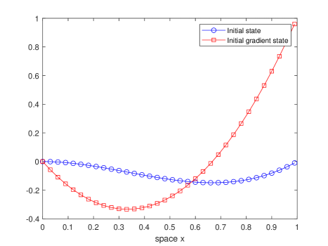
Figure 1: The initial state and initial gradient state of system (20) behavior, for $q=0.9$.

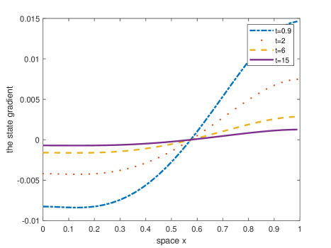
Figure 2: The gradient state of system (20) evolution, with $q=0.9$, for instants $t=0.9$, $t=2$, $t=6$, and $t=15$.

From Figure 1, we note that the state gradient is unstable at the initial instant $t=0$. However, Figure 2 shows that the state gradient of system (20) evolves close to zero when time $t$ increases. Moreover, it is stabilized by the feedback law (21), from the instant $t=15$, with the gradient stabilization error equal to $4.1\times 10^{-3}$.

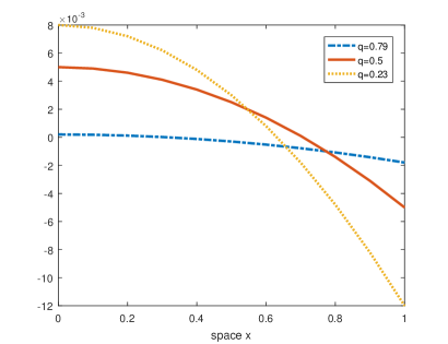
Figure 3: The gradient state of system (20) evolution, at the instant $t=20$, for $q=0.79$, $q=0.5$ and $q=0.23$.

Fractional order $q$	Gradient stabilization error
$q=0.1$	$1.9142$
$q=0.23$	$8.718\times 10^{-1}$
$q=0.5$	$1.428\times 10^{-1}$
$q=0.65$	$4.49\times 10^{-2}$
$q=0.79$	$1.25\times 10^{-2}$
$q=0.9$	$3.2\times 10^{-3}$

Table 1: The gradient stabilization error of system (20) for some value of the fractional order $q$ at $t=20$.

Table 1 presents the variation effect of the fractional order $q$ of system (20) on the state gradient stabilization error at a fixed instant $t=20$. We see that the gradient stabilization error decreases when the value of the fractional order $q$ increases. This is also illustrated by Figure 3 in the case of the fractional orders $q=0.79$, $q=0.5$ and $q=0.23$.

5 Conclusion

In this paper, the state gradient stability and stabilization of Caputo fractional diffusion systems are introduced. Sufficient conditions to obtain the gradient Mittag-Leffler and strong stability are investigated. Also, according to the conditions verified by the state space and those verified by the dynamic of the fractional linear system, the decomposition method is applied to characterize the state gradient stabilizing feedback law. Furthermore, in order to validate our developed results, a numerical example with simulations is provided.

Several questions are still open and deserve further investigations. This is the case, for example, of studying the gradient stabilization of fractional diffusion systems involving other kinds of fractional derivatives with singular and nonsingular kernels, including the Riemann–Liouville fractional derivative, the Caputo–Fabrizio fractional derivative, the weighted Atangana–Baleanu fractional derivative, the power and tempered fractional derivatives, etc. It would be also interesting to extend our Mittag-Leffler and strong gradient stabilization results to nonlinear fractional distributed systems. This is under investigation and will be addressed elsewhere.

Declarations

Conflict of interest

The authors declare no conflict of interest.

Data availability

The manuscript has no associated data.

Acknowledgements

Zitane and Torres are supported by The Center for Research and Development in Mathematics and Applications (CIDMA) through the Portuguese Foundation for Science and Technology (FCT – Fundação para a Ciência e a Tecnologia), projects UIDB/04106/2020 (https://doi.org/10.54499/UIDB/04106/2020) and UIDP/04106/2020 (https://doi.org/10.54499/UIDP/04106/2020).

References

• [1] E. E. Adams  and L. W. Gelhar, Field study of dispersion in a heterogeneous aquife: 2, Water Resources Res. 28 (1992), 3293–3307.
• [2] H. Berestycki, J. M. Roquejoffre  and L. Rossi, The periodic patch model for population dynamics with fractional diffusion, Discrete Contin. Dyn. Syst. Ser. S. 4 (2011), no. 1, 1–13.
• [3] W. Chen, Y. Liang, S. Hu  and H. Sun, Fractional derivative anomalous diffusion equation modeling prime number distribution, Fract. Calc. Appl. Anal. 18 (2015), no. 3, 789–798.
• [4] J. Cortés, A. V. D. Schaft  and P. E. Crouch, Characterization of gradient control systems, SIAM J. Control Optim. 44 (2005), no. 4, 1192–1214.
• [5] K. J. Engel and R. Nagel, One-parameter semigroups for linear evolution equation, Graduate Texts in Mathematics 194, Springer-Verlag New York, 2000.
• [6] F. Gao and H. Zhan, Boundedness and exponential stabilization for time–space fractional parabolic–elliptic Keller–Segel model in higher dimensions, Applied Mathematics Letters 144, (2023).
• [7] F. Ge, Y. Chen  and C. Kou, On the regional gradient observability of time fractional diffusion processes, Automatica 74 (2016), 1–9.
• [8] F. Ge, Y. Chen  and  C. Kou, Regional gradient controllability of sub-diffusion processes, J. Math. Anal. Appl. 440 (2016), no. 2, 865–884.
• [9] F. Ge, Y . Chen  and C. Kou, Regional Analysis of Time-Fractional Diffusion Processes, Springer: Cham, Switzerland, 2018.
• [10] M. Ginoa, S. Cerbelli  and  H. E. Roman, Fractional diffusion equation and relaxation in complex viscoelastic materials, Phys. A. 191 (1992), 449–453.
• [11] R. Gorenflo, A. A. Kilbas, F. Mainardi  and  S.V. Rogosin, Mittag-Leffler functions, related topics and applications, Springer, Berlin, 2014.
• [12] J. Huang  and   H. Zhou, Boundary stabilization for time-space fractional diffusion equation, European Journal of Control 65, (2022).
• [13] T. Kato, Perturbation Theory for Linear Operators, New York: Springer-Verlag, 1980.
• [14] S. R. Kessell, Gradient modelling: resource and fire management, Springer Science & Business Media, 2012.
• [15] A. A. Kilbas, H. M. Srivastava  and  J. J. Trujillo, Theory and applications of fractional differential equations, Elsevier Science Limited, 2006.
• [16] U. Kirsch, Structural Optimization: Fundamentals and Applications, Springer-Verlag Berlin Heidelberg, 1993.
• [17] F. List, K. Kumar, I.S. Pop  and F. A. Radu, Rigorous upscaling of unsaturated flow in fractured porous media, SIAM J. Math. Anal. 52 (2020), no. 1, 239–276
• [18] F. Mainardi, On some properties of the Mittag-Leffler function $E_{q}(-t^{q})$, completely monotonic for $t>0$ with $0<q<1$, Discret. Contin. Dyn. Syst. Ser. B. 19 (2014), no. 7, 2267–2278.
• [19] K. Sakamoto  and  M. Yamamoto, Initial value/boundary value problems for fractional diffusion-wave equations and applications to some inverse problems, J. Math. Anal. Appl. 382 (2011), no. 1, 426–447.
• [20] X.Y. Ye  and  C.J. Xu, A fractional order epidemic model and simulation for avian influenza dynamics, Math. Methods Appl. Sci. 42 (2019), no. 14, 4765–4779.
• [21] E. Zerrik  and  Y. Benslimane, An output gradient stabilization of distributed linear systems approaches and simulations, Intell. Control Autom. 3 (2012), no. 2, 159–167.
• [22] M. A. Zaitri, H. Zitane  and D. F. M. Torres, Pharmacokinetic/Pharmacodynamic anesthesia model incorporating psi-Caputo fractional derivatives, Comput. Biol. Med. 167 (2023), Paper No. 107679. arXiv:2311.05715
• [23] H. Zitane, A. Boutoulout  and  D.F.M. Torres, The stability and stabilization of infinite dimensional Caputo-time fractional differential linear systems, Mathematics 8 (2020), no. 3, Art. 353, 1–14. arXiv:2003.03085
• [24] H. Zitane, F.Z. El Alaoui  and  A. Boutoulout, Stability analysis of fractional differential systems involving Riemann-Liouville derivative, In: Nonlinear Analysis: Problems, Applications and Computational Methods, pp. 179–193, 2021.
• [25] H. Zitane, R. Larhrissi  and  A. Boutoulout, On the fractional output stabilization for a class of infinite dimensional linear systems. In: Recent Advances in Modeling, Analysis and Systems Control: Theoretical Aspects and Applications, pp. 241–259, 2020.