Continuous Design and Reprogramming of Totimorphic Structures for Space Applications

Abstract

Recently, a class of mechanical lattices with reconfigurable, zero-stiffness structures has been proposed, called Totimorphic structures. In this work, we introduce a computational framework that allows continuous reprogramming of a Totimorphic lattice’s effective properties, such as mechanical and optical properties, via continuous geometric changes alone. Our approach is differentiable and guarantees valid Totimorphic lattice configurations throughout the optimisation process, thus providing not only specific configurations with desired properties but also trajectories through configuration space connecting them. It enables re-programmable structures where actuators are controlled via automatic differentiation on an objective-dependent cost function, altering the lattice structure at all times to achieve a given objective – which is interchangeable to achieve different functionalities. Our main interest lies in deep space applications where harsh, extreme, and resource-constrained environments demand solutions that offer flexibility, resource efficiency, and autonomy. We illustrate our framework through two proofs of concept: a re-programmable metamaterial as well as a space telescope mirror with adjustable focal length, both made from Totimorphic structures. The introduced framework is easily adjustable to a variety of Totimorphic designs and objectives, providing a light-weight model for endowing physical prototypes of Totimorphic structures with autonomous self-configuration and self-repair capabilities.

Keywords morphing structure  $\cdot$ deployable structure  $\cdot$ multi-functional metamaterial  $\cdot$ totimorphic  $\cdot$ programmable material  $\cdot$ inverse design  $\cdot$ automatic differentiation  $\cdot$ in-orbit deployment  $\cdot$ space infrastructure  $\cdot$ telescope

1 Introduction

Throughout nature, the intricate and disordered lattice structures that are observed in bones, plant stems, dragonfly wings, coral, radiolarians [1], amongst many other examples, demonstrate how powerful geometry is for designing structures with extreme mechanical properties from a very limited selection of base materials [2]. Metamaterials [3] are a recent example of human-engineered lattice structures that utilise the geometric design space of unit cells to change the properties of the lattice obtained by tiling this motive, often producing structures with different properties than those of the underlying lattice material – for instance, having a soft and compressible lattice made of a very brittle material such as ceramic [4]. In addition to metamaterials that follow a periodic design philosophy, there is a growing interest in (inversely) designing disordered lattice materials and structures [5, 6, 7, 8, 9, 10, 11, 12], allowing us to fully tap into the functional design space explored by nature. Since lattices can be constructed using additive manufacturing, they combine ease of manufacturing with a highly expressive design space that only requires a small amount of building materials. It is not surprising that lattices have found applications on a variety of scales, ranging from nano- and mesoscale materials to large-scale structures such as space habitats [13, 14, 15, 16]. The static nature of lattices also means that once they have been constructed, their properties are fixed – unless physically stimulating the lattice changes the properties of its base materials or allows switching between different shapes (e.g., magnetically [17, 18, 19]), therefore enabling a certain degree of reprogrammability of the lattice’s properties; also known as active metamaterials [20, 21].

Recently, a type of reconfigureable lattice called a Totimorphic structure has been proposed and demonstrated in a physical prototype [22]. The Totimorphic property of these lattice structures enables the continuous alteration of effective properties of the lattice through mechanically induced continuous geometric changes alone. Totimorphic lattices are made of a triangle-shaped unit cell composed of a beam (Fig. 1.A, points $\mathrm{A}$ to $\mathrm{B}$), a lever that connects via a ball joint to the middle of the beam (Fig. 1.A, points $\mathrm{P}$ to $\mathrm{C}$), and two zero-length springs that connect the two ends of the beam with the other end of the lever (Fig. 1.A, $\mathrm{A}$ to $\mathrm{C}$ and $\mathrm{B}$ to $\mathrm{C}$). Due to the zero-length property of the springs, the Totimorphic unit cell implements a mechanical version of Thales’s theorem: in any given lever position (lying on a half-circle), the forces from the springs pulling at the lever combine such that the total force is parallel to the lever orientation, resulting in no torque on the lever. Consequently, the unit cell in this state is neutrally stable: it is completely compliant to reconfiguration but will not move in the absence of external forces.

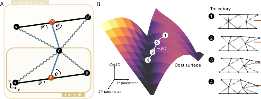
Figure 1: Illustration of Totimorphic lattices. (A) Totimorphic unit cell and elementary cell used for the tile, as defined in this work. (B) Actuation of angles (or lattice dynamics) are defined as gradient descent on an objective-dependent cost function. This way, both a lattice configuration with a desired property is found as well as the trajectory connecting it to the initial configuration. The surface plot represents the cost for different configurations. An example trajectory following the gradient $-\nabla C$ is shown in white, and the corresponding lattice configurations to the right. For illustration purposes, the task here is to move the upper right corner of the lattice (blue dot) to the height of the red line. In more realistic scenarios, the landscape might contain insurmountable barriers, because the lattice needs to break in order to move between certain configurations.

Mathematically, the Totimorphic unit cell is characterised by a set of three geometric constraints, which we call Totimorphic condition in the remainder of the paper. The three constraints are as follows:

1. The beam has a fixed length $l_{\text{b}}$.

2. The lever has a fixed length $\frac{1}{2}l_{\text{b}}$.

3. The lever is connected at one end to the midpoint of the beam.

A Totimorphic unit cell is only allowed to transform through configurations that satisfy these constraints. When assembling unit cells into a lattice structure, it can morph into different shapes by adjusting beam and lever orientations as long as each unit cell satisfies the Totimorphic condition and unit cells stay connected, i.e., the lattice does not break.

In previous work [22], the lattice is usually initialised as a flat surface. A desired surface shape is then found by optimising the lattice point positions using an objective-dependent, quadratic cost function, with the Totimorphic condition being accounted for as non-linear constraints. However, this comes with two limitations: firstly, the Totimorphic condition is never satisfied exactly, but only up to a certain error. Secondly, this approach only provides the final configuration with the desired shape, not the trajectory through configuration space to get there – or more simply put, we do not know how to morph from the initial to the found configuration without breaking the lattice. In the introduced approach, we avoid these problems by formulating the reconfiguration of Totimorphic lattices as an unconstrained optimisation problem. This is achieved by choosing a new set of parameters $\mathcal{P}$ to describe the lattice, from which the physical coordinates $\mathcal{R}$ (beam and lever ends, i.e., points $\mathrm{A}$, $\mathrm{B}$, $\mathrm{P}$, $\mathrm{C}$, and primed variants) of the lattice are calculated analytically, $\mathcal{R}=f_{\mathrm{T}}(\mathcal{P})$. These new parameters are chosen such that the map $f_{\mathrm{T}}$ from new to physical lattice coordinates always satisfies the Totimorphic condition. We derive new parametrisations and suitable maps both for lattices in two and three-dimensional space. Although this can be easily applied to any Totimorphic lattice, we illustrate it for a specific tiling used in [22] where the lattice is formed from hour-glass shaped cells (made from two Totimorphic unit cells), see Fig. 1.A. We call these cells elementary cells in the remainder to distinguish them from unit cells.

The utilized approach is known in analytical mechanics as generalized coordinates, which is often used to describe mechanical systems with constraints, or as the substitution method in mathematical optimisation. In our case, the chosen generalized coordinates are all real-valued and, different from the physical lattice coordinates, bounded. Additionally, we find that the map $f_{\mathrm{T}}$ is differentiable, and hence automatic differentiation (i.e. gradient descent) can be used to optimize cost functions written in terms of lattice and generalized coordinates. Consequently, performing gradient descent on the cost function is equivalent to following a trajectory through configuration space that morphs the lattice into a configuration exhibiting a desired mechanical or optical property without breaking it (Fig. 1.B); which can be efficiently and robustly realised using modern automatic differentiation libraries such as pyTorch. In other terms: when interpreting a Totimorphic lattice as a dynamic system that reconfigures continuously, its dynamics (or actuations) are given by the gradient of the cost function. Thus, our approach provides not only a target lattice configuration with desired properties, but also the trajectory connecting the initial lattice configuration with the target one.

We use the introduced framework to explore new application areas for Totimorphic lattices. Different from previous work which only focused on shape shifting [22], we optimise the topology of Totimorphic lattices to continuously change its effective material properties. Specifically, we propose Totimorphic structures as deployable and reconfigurable meso - and macro-scale space infrastructure, where the focus lies on adapting the functionality of the structure through autonomous reconfiguration.

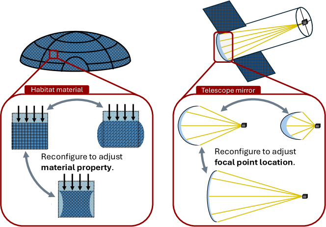
Figure 2: Totimorphic structures as building blocks of, e.g., space habitats, spacecraft components, and tools with reprogrammable properties. In this work, we specifically look into lattice structures that can alter their mechanical properties, i.e., how they behave under stress. In addition, we explore the concept of using Totimorphic structures as the backbone of large-scale space infrastructures such as space telescopes – not only to ease their deployment, but to equip them with reprogrammable properties as well. For example, we demonstrate a mirror element that can adjust its surface shape to alter the location of its focal point.

Several designs of reprogrammable materials have recently been proposed and verified in the aerospace field, with related examples being Mechanical Neural Networks [23] – lattices with programmable stiffness of each beam elements – and the Trimorph origami pattern [24] – an origami structure with triclinic symmetry that can transition between multiple discrete stable states with different mechanical properties such as Poisson’s ratios with opposite signs. As a first use case, we demonstrate Totimorphic lattices with continuous mechanical properties (Fig. 2, left), meaning that effective properties such as Poisson’s ratio or stiffness can be adjusted continuously through continuous changes in the configuration of the Totimorphic lattice, i.e., lever and beam orientations obtained via gradient descent.

As a second use case, we apply our framework to large scale space structures and spacecraft such as space telescopes, antennas, and habitats. A variety of futuristic concepts have recently been proposed to reduce the costs and risks of launching and deploying large space infrastructure. Particularly prominent ones are the use of formation flight [25, 26], CubeSat swarms that assemble and reconfigure by docking into static formations, e.g., to form space telescope mirrors [27], autonomously assembling tiles for in-orbit habitat construction [26, 28], Origami techniques to unfold spacecraft components [29, 30], as well as robotic systems for ground-based habitat construction on other celestial bodies [15]. Since a major constraint for the possible size and structure of spacecraft is the launcher used for deployment in orbit or deep space, such concepts are in action already, e.g., the James Webb Space Telescope was folded together for launch and subsequently unfolded. However, most concepts focus only on deployment, restricting (or at least severely limiting) any further reconfiguration of the spacecraft after deployment to adapt to changing mission parameters or changes in the environment the spacecraft is operating in. Here, we propose that Totimorphic lattices represent an intriguing candidate to form the backbone of deployable and reconfigurable large-scale space infrastructure. As a proof of concept, we use our framework to construct a Totimorphic mirror with reconfigurable focal length as well as self-repair capabilities (Fig. 2, right).

In summary, we introduce a computational framework for autonomously reconfiguring Totimorphic structures for different functional tasks, focusing on adapting the effective properties of lattices by changing only their geometric structure. Reconfiguration is realized as gradient descent minimizing an objective-dependent cost function, therefore enabling continuous movement through the configuration space of Totimorphic lattices to adjust their properties. We further highlight and validate in simulation the applicability of this framework in the space domain, adding to the growing number of concepts of self-constructing and reconfigurable designs crucial for future uncrewed deep space exploration.

2 Results

In the following, we first introduce how the generalised coordinates of a Totimorphic lattice are chosen and how they are used to analytically calculate the physical coordinates of the lattice elements. After introducing the model, we present the results of two proofs of concept: a meso-scale lattice material with continuously programmable material properties, as well as a large-scale space telescope with continuously adjustable optical properties. Mathematical details on all models can be found in Section 4. Simulation details are in the supplemental information.

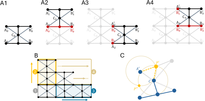
Figure 3: Parametrizing Totimorphic lattices. (A) When connecting elementary cells to an existing lattice, overlapping elements are shared with already existing cells (shown in red). Thus, the number of degrees of freedom of the newly added cell is reduced. (B) Iterative construction of a lattice made of Totimorphic cells. (C) If all points except one in an elementary cell are predetermined (shown in blue), the remaining point is obtained from the Totimorphic condition. This is illustrated here for the case where $\mathrm{A^{\prime}}$ and $\mathrm{C}$ are given. Since $\mathrm{P^{\prime}}$ is connected via a beam and lever to these points, it has to be a distance of $\frac{1}{2}l_{\text{b}}$ away from both. The solution to this problem is given by the intersection points of two circles, or equivalently, by a quadratic equation. Two points $\mathrm{P^{\prime}}$ and $\mathrm{P}^{\prime\prime}$ satisfy the Totimorphic condition, however, the latter would reverse the order of $\mathrm{A^{\prime}}$ and $\mathrm{B^{\prime}}$ and is therefore not a valid physical solution.

2.1 Degrees of freedom in Totimorphic lattices

To model Totimorphic lattices, we absorb the Totimorphic condition into the parameters used to describe the lattice’s configuration. The minimum number of parameters needed to uniquely capture the lattice is given by its degrees of freedom $df$. In general, the degrees of freedom of an elementary cell in a Totimorphic lattice are determined by three factors: the freely moving points characterising the cell itself, the Totimorphic condition, and points that overlap with other cells in the lattice – with the latter two factors reducing the number of degrees of freedom. In the following, we construct a lattice cell by cell to identify how a cell’s degrees of freedom depend on where and when it is added to the lattice. For simplicity, we showcase this for lattices in two dimensions:

1. The first elementary cell that we add is not constrained by any neighbouring cells (Fig. 3.A1). It is characterised by five points: $\mathrm{A}_{0}$, $\mathrm{B}_{0}$, $\mathrm{C}_{0}$, $\mathrm{A}^{\prime}_{0}$, and $\mathrm{B}^{\prime}_{0}$. In two dimensions, this yields ten parameters (two for each point). However, due to the Totimorphic condition, i.e. the constant lengths of the four beams, there are only six degrees of freedom (each length constraint reduces the degrees of freedom by one), and so we only require six parameters to fully describe the elementary cell.

2. Adding another elementary cell above the first one, the points $\mathrm{A}_{1}$ and $\mathrm{B}_{1}$ are already determined, $\mathrm{A}_{1}=\mathrm{A}^{\prime}_{0}$ and $\mathrm{B}_{1}=\mathrm{B}^{\prime}_{0}$ (Fig. 3.A2). Thus, we have six parameters (point $\mathrm{C}_{1}$, $\mathrm{A}^{\prime}_{1}$ and $\mathrm{B}^{\prime}_{1}$), which leaves us with three degrees of freedom for this elementary cell when accounting for the three remaining length constraints (two levers and one beam). The same is true when adding an elementary cell below the first one.

3. Adding another elementary cell to the right of the first one, both points $\mathrm{A}_{2}$ and $\mathrm{A}^{\prime}_{2}$ are already determined, $\mathrm{A}_{2}=\mathrm{B}_{0}$ and $\mathrm{A}^{\prime}_{2}=\mathrm{B}^{\prime}_{0}$ (Fig. 3.A3). Since all four length constraints (two levers and two beams) still have to be enforced, we are left with only two degrees of freedom in this case. The same is true when adding an elementary cell to the left of the first one.

4. Adding an elementary cell above and to the right of two other cells, the points $\mathrm{A}_{3}$, $\mathrm{B}_{3}$ and $\mathrm{A}^{\prime}_{3}$ are already determined, $\mathrm{A}_{3}=\mathrm{B}^{\prime}_{0}$, $\mathrm{B}_{3}=\mathrm{B}^{\prime}_{1}$, $\mathrm{A}^{\prime}_{3}=\mathrm{B}^{\prime}_{1}$ (Fig. 3.A4). Since three length constraints still have to be satisfied, we are left with only one degree of freedom (four from the remaining points minus the three length constraints). This is in general true when adding an elementary cell such that two of its adjacent sides are connected to other elementary cells.

Following the above logic, we find that for a lattice in two dimensions, the first placed elementary cell has six degrees of freedom, elementary cells to the left and right of the first one have two each, cells above and below have three each, and all other elementary cells have only one. For a lattice with $C$ columns and $R$ rows, this results in $df_{\mathrm{2D}}=2+C+2R+C\cdot R$ degrees of freedom in total. Applying the same logic to a lattice in three dimensions yields eleven, five, six, and three degrees of freedom, respectively, or $df_{\mathrm{3D}}=3+2C+3R+3C\cdot R$ in total.

2.2 Angle-based generalised coordinates

In this work, we parameterise all elementary cells using beam and lever angles and a vector indicating the location of the whole lattice in space. In addition, we construct a lattice by placing the bottom left elementary cell first and adding all other elementary cells row by row. We briefly illustrate this process in two dimensions:

1. As the first step, we place the bottom left corner elementary cell of the lattice, which has six degrees of freedom (Fig. 3.B, box 1). The six parameters we choose to describe this elementary cell are the location of the lattice and the orientation of the bottom and top beams and levers.

2. Then we add the first column, i.e. we stack up elementary cells on top of the first one (Fig. 3.B, box 2). Each elementary cell in this column has three degrees of freedom. Here, we choose the orientation of bottom and top lever as well as the orientation of the upper beam as parameters.

3. We then add the first row, i.e. we string together elementary cells to the right of the first one (Fig. 3.B, box 3). These elementary cells only have two degrees of freedom, which we choose to be the orientation of the bottom beam and lever. In this case, the midpoint of the upper beam ($\mathrm{P^{\prime}}$) is given by the (analytic) solution of a quadratic equation representing the Totimorphic condition (Fig. 3.C), see Section 4.2.2 for details.

4. Then we fill in the remaining elementary cells row-wise from left to right (Fig. 3.B, box 4). All these elementary cells have only one degree of freedom, which we choose to be represented by the orientation of the lower lever. The midpoint of the upper beam is again given by the solution of a quadratic equation.

For a detailed mathematical description, see Section 4.2. Although we parametrise the lattice using beam and lever angles here, many other parametrisations are possible. From the quadratic equations, we further derive upper and lower bounds for the lever angles, allowing levers to be pushed or dragged by other lattice elements (Section 4.2.3). For lattices in two dimensions, additional conditions are derived to avoid configurations with overlapping lattice elements (Section 4.2.3). Models of lattices in three dimensions are constructed analogously (Section 4.3).

With this approach, a Totimorphic lattice is represented by a set of $df$ parameters $\mathcal{P}$, $|\ \mathcal{P}\ |=df$, which in our case is the location of the lattice’s bottom left corner in space as well as the angles of levers and beams in the lattice. From this set of parameters, there exists a differentiable function $f_{\mathrm{T}}$ which maps to the points of each elementary cell in the lattice (lever and beam endings), i.e. $\mathcal{R}=f_{\mathrm{T}}(\mathcal{P})$, where $\mathcal{R}$ is a set of vectors containing the coordinates of each point in the lattice – we call this the Totimorphic model in the following. Invalid lattice configurations are given by values of the generalised coordinates $\mathcal{P}$ for which no solution of $f_{\mathrm{T}}$ exists, which can be checked using simple criteria. Note that, similar to how in a neural network outputs are calculated layer by layer, points are calculated elementary cell by elementary cell; with points of later elementary cells (i.e. higher row or further to the right) depending on the configurations of elementary cells that came before. This way, a point in, e.g., the uppermost layer can be moved into a desired target position by changing the angles of elementary cells in the bottom layer.

To change the configuration of the lattice to one with some desired property (e.g. a desired stiffness), we minimise an objective-dependent cost function that measures how well the current configuration satisfies the desired property. In most cases, we express the cost function using the point coordinates obtained from the Totimorphic model. What is actually being optimised, however, are the parameters $\mathcal{P}$ used to characterise the lattice; generally these parameters number far less than the physical lattice coordinates. By tracking intermediate configurations, we also get the trajectory through parameter space connecting the initial and the final lattice configuration – which is a major benefit compared to previously employed methods [22]. In this work, we exclusively use automatic differentiation (i.e. gradient descent) as our optimisation algorithm of choice to guarantee scalability, but other techniques can be used as well. To demonstrate the introduced framework, we focus on use cases where effective properties of the lattice have to be optimised, i.e. global properties of the lattice structure. As a first proof of concept, we explore reconfigurable lattice structures with adjustable mechanical properties, namely the Poisson’s ratio which characterises how a mechanical lattice responds when compressed. As a second proof of concept, we demonstrate a deformable telescope mirror made from a Totimorphic lattice capable of continuously adjusting the location of its focal point.

2.3 Continuous inverse design of lattice structures

In the following, we use the introduced framework to continuously change the Poisson’s ratio of a mechanical lattice (on the length scale of cm) through continuous changes of the Totimorphic configuration. The used approach is based on the work and simulation code presented in [9], where effective mechanical properties of disordered lattices were optimised by adjusting the lattice topology using a differentiable framework.

To predict the mechanical properties of a Totimorphic lattice, we use the direct stiffness method (see Section 4.4) to set up a compression experiment (see Section 4.4.2). In a compression experiment, the lattice is glued between surfaces and slowly compressed. During compression, the response of the lattice to this load is measured, for example, the displacement of nodes in the lattice – from which mechanical properties such as effective stiffness and Poisson’s ratio are derived. Here, we restrict the work to the effective Poisson’s ratio, which measures how a material expands on average horizontally when compressed vertically (see Section 4.4.3). A positive Poisson’s ratio (like honeycomb tiles) means the material widens, while a negative one means it narrows (also known as auxetic). A Poisson’s ratio of zero consequently means that the material does not change its width during compression.

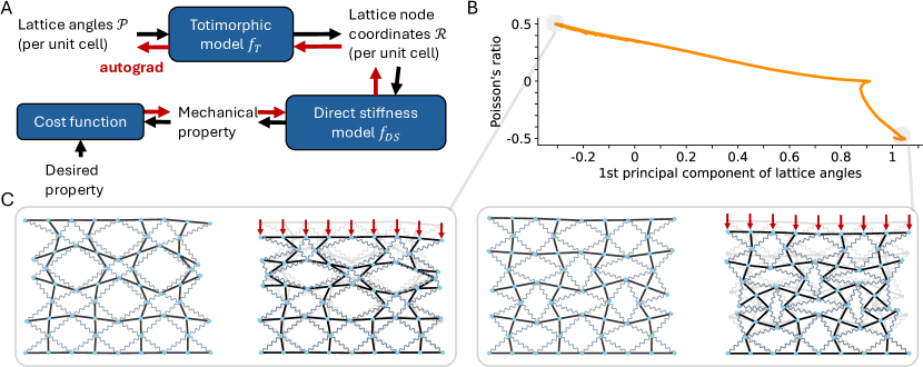
Figure 4: Inverse design of mechanical properties of Totimorphic lattices. (A) Schematic of the inverse design pipeline. (B) During optimisation, we obtain a continuous trajectory through configuration space (here represented using the first principal component of the angles representing the lattice) connecting the initial configuration ($\nu=0$) and the two final configurations ($\nu=\pm 0.5$). Since the lattice always fulfills the Totimorphic condition, it passes through all intermediate Poisson’s ratios while morphing. (C) Illustration of the final design for $\nu=0.5$ (left) and $\nu=-0.5$ (right), shown without (left) and with load (right, red arrows).

For the direct stiffness approach, we only consider beam and lever elements in the lattice, as they are the major supporting elements of the lattice. We model these using Generalized Euler-Bernoulli beam elements [31] (see Section 4.4.1). Furthermore, we assume that joints in the Totimorphic lattice are locked during the compression experiment, meaning that the parameters $\mathcal{P}$ are not changed while applying a load. To do a single step of the compression experiment, we first calculate the stiffness matrix from the lattice points $\mathcal{R}$. Using the stiffness matrix, we can then derive the displacement of each node in the lattice resulting from the compression by solving a linear equation. We repeat this process several times and note down the horizontal and vertical strain (mean length change). Finally, the Poisson’s ratio, which is defined as the slope of the strain-strain curve, is obtained via linear regression. This process can be formalized as a single differentiable function $f_{\mathrm{DS}}$ which takes as input the coordinates of the lattice nodes and returns the Poisson’s ratio $\nu=f_{\mathrm{DS}}\left(f_{\mathrm{T}}(\mathcal{P})\right)$. The trajectory in parameter space (i.e., parameter changes $\Delta\mathcal{P}$) to reconfigure the lattice until it has a desired target Poisson’s ratio $\nu^{\mathrm{tgt}}$ is then obtained by descending the gradient of the cost function $C$,

$$C(\mathcal{P})= \|\nu^{\mathrm{tgt}}-f_{\mathrm{DS}}\left(f_{\mathrm{T}}(\mathcal{P})\right)\|_{1}\,,$$ (1)

$$\Delta \mathcal{P}\propto-\nabla_{\mathcal{P}}C(\mathcal{P})\,,$$ (2)

where $\|\cdot\|_{1}$ is the L1 norm. Further details about the mathematical formulation of the direct stiffness method and the Poisson’s ratio can be found in Section 4.4. The whole optimisation pipeline is illustrated in Fig. 4.A.

We demonstrate this approach for a $4\times 4$ Totimorphic lattice with beam length $l_{\text{b}}=1\,\mathrm{cm}$, beam cross-area $A=4\,\mathrm{mm}^{2}$, Young’s modulus of the beam material of $E=1\,\mathrm{GPa}$ (around the order of magnitude of polymers), and second moment of area $I=\frac{A^{2}}{12}$ (representing a square-shaped cross-sectional area). The initial lattice has a Poisson’s ratio of approximately zero, which is not surprising as it resembles a square lattice. From this initial configuration, we perform gradient descent to get to a configuration with Poisson’s ratio $\nu^{\mathrm{tgt}}=\pm 0.5$. This results in two trajectories starting from the initial configuration and ending at a configuration with the desired Poisson’s ratio, shown in Fig. 4.B using the first principal component of the lattice parameters $\mathcal{P}$. The final lattice configurations and their response to applying load is shown in Fig. 4.C. In case of the configuration with positive Poisson’s ratio (Fig. 4.C, left), large pockets were formed that widen during compression. In case of negative Poisson’s ratio (Fig. 4.C, right), the resulting lattice geometry is composed of square-shaped elements (one beam and two levers surrounded by springs) that pivot inwards when compressed from above. This effect is most pronounced in the lower half of the lattice structure. Similar designs were obtained for larger lattices, e.g., $8\times 8$ trained to achieve even higher Poisson’s ratios (see supplemental information). It is worthy noticing that every intermediate configuration obtained during optimisation is a legitimate Totimorphic lattice, and hence we are capable of continuously adjusting the Poisson’s ratio by continuously changing the lattice angles. For an animation of the reconfiguration process and the compression experiment (after reconfiguration), see Video S1a,b and Video S2a,b.

2.4 Deployable and reconfigurable large-scale structures

In the following, we envision that the Totimorphic lattice (on the length scale of meters) acts as a skeleton for, e.g., a graphene sheet that forms the reflective surface of a primary mirror of a space telescope [32]. We assume a $6\times 6$ Totimorphic lattice with $l_{\text{b}}=1$m in its flat surface configuration. By only changing the lever angle of all elements in the lattice (i.e., setting them all to the same value), we can switch from the flat surface configuration to a collapsed one (and vice versa), greatly reducing the surface area and volume required to launch the Totimorphic structure (see Fig. 5). The reduction in surface area is given by $\sin\theta_{\mathrm{min}}$, where $\theta_{\mathrm{min}}$ is the minimum angle the levers can be set to physically. Consequently, for launching, the lattice is configured in its collapsed configuration and for deployment, the lever angles are slowly increased to unfold the lattice into a flat surface.

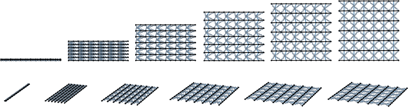
Figure 5: Deployment of a Totimorphic lattice structure. A Totimorphic sheet reconfigures from its collapsed (left) to its unfolded (right) configuration by raising all levers. The unfolding is shown from two different perspectives.

After deployment, the lattice configuration is continuously adjustable to change the optical properties of its mirror surface. In our case, the goal is to focus the light onto a secondary optical element such as a detector or a secondary mirror located at point $\boldsymbol{f}^{\mathrm{tgt}}$, which we call the target focal point in the following (Fig. 6.A). We utilise a similar approach as for the material inverse design use-case, meaning that we construct a differentiable framework that allows us to find suitable lattice configurations (and trajectories connecting them) using gradient-based optimisation. First, for simplicity, we assume that each unit cell reflects light at the mid-point of the lever in simulations (i.e., the mid-point between $\mathrm{C}$ and $\mathrm{P}$ as well $\mathrm{C}$ and $\mathrm{P^{\prime}}$, see Fig. 6.A). In addition, we assume that the object to be imaged is far away such that the incoming light is parallel. Given an incidence direction $\boldsymbol{I}$ ($\|\boldsymbol{I}\|_{2}=1$, where $\|\cdot\|_{2}$ is the Euclidean norm) of the incoming light, the direction of the reflected light originating from each unit cell $(ij)$ is calculated using ray-based optics (see Section 4.5.1). Subsequently, we obtain the point where each reflected light ray is closest to the target focal point (see Section 4.5.2). The whole calculation can again be formulated as a series of differentiable operations, which we summarise in two functions: the Totimorphic model ($f_{\mathrm{T}}$), and the optics part $f_{\mathrm{O}}$, such that $\boldsymbol{F}=f_{\mathrm{O}}(f_{\mathrm{T}}(\mathcal{P}))$ is a list of vectors containing the closest point to $\boldsymbol{f}^{\mathrm{tgt}}$ on each reflected light ray.

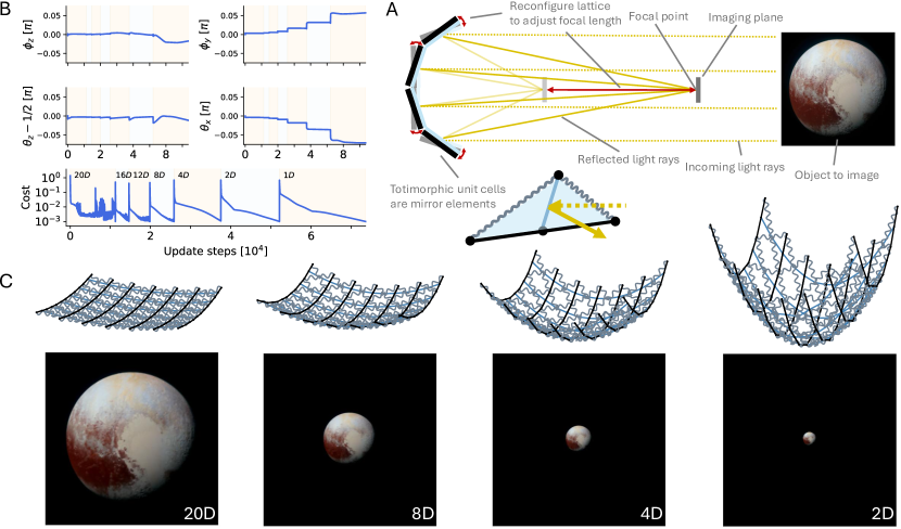
Figure 6: Deployment and reconfiguration of a Totimorphic telescope mirror. (A) Schematic of the studied setup. Given an object to be imaged, the unit cells of the Totimorphic lattice are used as mirror elements to focus the light on an imaging plane. By changing the lattice configuration, the focal point and focal length are adjusted.(B) Reconfiguration of the lattice to several different focal lengths, starting from a flat configuration. A few parameters as well as the objective-dependent cost are shown. (C) Lattice configuration and images received when using the lattice as a mirror, for configurations featuring different focal lengths.

To find a Totimorphic configuration that focuses the light in a desired target focal point $\boldsymbol{f}^{\mathrm{tgt}}$, we again optimise the parameters characterising the Totimorphic lattice using gradient descent on a task-dependent cost function $C$,

$$C(\mathcal{P})=\sum_{\mathrm{unit\ cells}\ i} \left\|\boldsymbol{f}^{\mathrm{tgt}}-f_{\mathrm{O}}\big{(}f_{\mathrm{T}}(\mathcal{P})\big{)}_{i}\right\|_{2}\,,$$ (3)

$$\Delta\mathcal{P}\propto -\nabla_{\mathcal{P}}C(\mathcal{P})\,,$$ (4)

During the optimisation process, we only present light coming from one direction (i.e., orthogonal to the initial lattice surface) which has to be focused into a single target point. In Fig. 6.B-C, we show how the Totimorphic lattice transforms – starting from a flat surface – into curved surfaces that focus the light into a single point at decreasing focal lengths given in multiples of the mirror diameter $D$. Fig. 6.B (bottom) shows the value of the cost function during deployment (from flat to a focal length of 20$D$, see supplemental figures) and during reconfiguration to new targets, i.e., focal lengths of 16, 12, 8, 4, 2, and 1$D$. In all cases, we reach the same cost after reconfiguring the lattice, which means that the light reflected from all unit cells is focused with a similar precision in the target focal points. In Fig. 6.B (top), a few lattice parameters are shown during the reconfiguration process, demonstrating that only minor continuous changes are required to achieve the desired result. The reconfiguration is further illustrated in Video S3a,b.

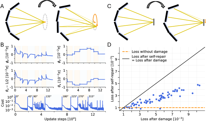
Figure 7: Off-center focus and self-repair capabilities. (A) The target focal point can be set off-center, which is shown here by guiding the focal point of the telescope on a circle around the original focal point. (B) Selected angle parameters of the lattice as well as the cost during the circular guidance experiment depicted in (A). During optimisation, several discrete target focal points at different angles on the circle were used. (C) Damage on one of the mirror elements (here: top) adds a deflection to light reflected by this element, thus putting it out of focus. Through reconfiguration of the lattice, the added deflection can be compensated for. (D) Result for self-repairing a single defect, repeated several times (blue dots). In each repetition, the damaged unit cell and the strength of the damage were selected randomly.

As a proof of concept, we use the Totimorphic lattice to image a real object; specifically, a photograph of Pluto at the same distance and angular extension of the Moon (as seen from Earth), see Fig. 6.A. To construct the image, we record where light coming from each pixel of the image hits the imaging plane after being reflected by the unit cells of the lattice – imitating the real process of image generation in a telescope (see Section 4.5.4 for details). The resulting image closely resembles the original object, resolving small details such as contours of icy regions on Pluto (Fig. 6.C). Moreover, as expected, decreasing the focal length of the Totimorphic mirror increases its field of view; enabling adaptive zoom-in and out by reconfiguring the lattice.

Although we only demonstrate reconfiguration for a few discrete focal lengths, in principle, the telescope can achieve a continuum of focal points by successively adjusting the target focal length. In addition, the telescope is not limited to focal points that are on the central axis of the telescope surface, as shown in Fig. 7.A-B where we guide the focal point on a circle around this axis using the above gradient-based optimisation.

The presented approach also allows to use reconfiguration of the lattice surface to compensate for defects introduced by mirror damage, e.g., through micrometeoroids [33]. We illustrate this by adding a single defect to one of the lattice’s unit cells (selected randomly), which is modelled by adding a deflection (randomly determined but static) to the light rays reflected from this cell (Fig. 7.C; see Section 4.5.3 for details). As before, we perform gradient descent on the respective cost function to find a lattice configuration that compensates for this defect (Fig. 7.C-D). This is studied for increasing degrees of damage, i.e., for increasing amounts of deflection. For all cases, the reconfiguration improves the performance of the mirror – although for more extreme damage, we are not able to return to the baseline performance from before the damage occurs. This is mainly because correcting for the damage requires an asymmetric configuration in the lattice, which is only possible to a limited degree before interfering with the focus capability of other (undamaged) unit cells. But still, for smaller amounts of damage, reconfiguration allows a return to baseline performance. In a realistic scenario, this could be realized in a "lattice-in-the-loop" setting, meaning that we use the actual lattice to collect where light from each unit cell hits the imaging plane, and then use the measurements in the backward pass to get the required parameter changes of the physical mirror, i.e., we use the simulation model as a proxy for the error calculation and simply replace predicted values – the distances to the focal point – with real measurements.

3 Discussion

We derived a reparametrisation of Totimorphic lattices in two and three dimensions that enables the use of constraint-free gradient descent to optimise the lattice topology. Different from previously proposed mechanically reprogrammable systems [23, 24], the effective physical properties of Totimorphic lattices can be changed continuously.

This was successfully illustrated using the introduced framework for two space-related applications: continuous control of the mechanical properties of a metamaterial as well as continuous control of the optical properties of a conceptual telescope mirror composed of Totimorphic unit cells.

Instead of reparametrising the lattice, a variety of other techniques can be applied as well [34]. As an example, for gradient-based optimisation the penalty method can be used where the Totimorphic condition is added as a penalty term in the cost function to be reinforced. However, it comes with the downside that the constraints are not perfectly satisfied during optimisation (hence we do not obtain trajectories), and in practice it can be non-trivial to avoid becoming stuck in local minima when trying to balance the penalty and the objective-dependent terms in the cost function. Another alternative is the method of Lagrange multipliers, but it does not work with gradient descent, requiring more involved solvers capable of finding saddle points of the cost function. An extension of the Lagrange multiplier method, called basic differential multiplier method [34], which is compatible with gradient descent can be used instead, although – as in the case of the penalty method – constraints are not satisfied throughout the whole optimisation process. Apart from methods using gradient descent, more advanced approaches that divide the problem into simpler sub-problems can be used, such as sequential quadratic programming [35]. In this work, we stick to the gradient-based approach, as it combines ease of formulation with a straightforward and flexible algorithmic implementation, which is scaleable to large lattices and more involved cost functions, e.g., including non-linear functions of the physical lattice coordinates such as deep neural networks. Most importantly, it defines proper dynamics driven by an objective-dependent cost function to reconfigure the lattice – something most other methods are lacking.

For the model in two dimensions, we were able to formulate simple rules for detecting when lattice elements collide during reconfiguration. In contrast, we did not employ any collision detection methods for the three-dimensional model, restricting our experiments to cases where strong folding of the lattice surface does not occur. In future work, approaches used to simulate textiles [36] could be employed to detect self-collisions in Totimorphic structures. Apart from simply detecting whether the structure collides with itself, it is even more important to deal with self-collisions and invalid lattice configurations during the optimisation process. A default method for dealing with collisions in, e.g., simulations of swarming robots [37] or textile simulations [36] is to add strong repulsive forces that only act between elements at very low distances. Adopting such an approach for Totimorphic structures is certainly feasible, but might be problematic due to the rigid and discontinuous nature of lattices. Furthermore, this method only helps in dealing with self-collisions and increases the computational cost of simulations substantially. Alternatively, one could truncate parameter updates during optimisation such that general invalid lattice configurations are avoided – although the optimisation process can get stuck trying to pass through invalid configurations, requiring either stochasticity to escape such local minima of the cost function or intermixing with optimisers that allow discontinuous changes of the lattice configuration. In the presented experiments, we only checked whether the lattice is still valid after each update and stopped in case the lattice broke.

Even though we only derived the model for a specific tiling here, the approach can be generalized to arbitrary Totimorphic structures. It further enables a theoretical study of Totimorphic designs. For example, it is an open question whether the Totimorphic configuration space is fully connected or consists of topologically disconnected sub-spaces; or put differently: it is not clear whether there always exists a continuous trajectory connecting two valid Totimorphic configurations. This is particularly important when utilising optimisation methods that – different to gradient descent – facilitate a global exploration of the configuration space, such as evolutionary strategies, to avoid selecting solutions that are not reachable from the initial lattice configuration.

In the first application, we demonstrated how a Totimorphic lattice can be reconfigured to continuously change it’s Poisson’s ratio from negative to positive values and vice versa. This was illustrated for two-dimensional truss lattices only. For three dimensional metamaterials, the same approach can be used by exchanging the two-dimensional Totimorphic model and direct stiffness method with their three-dimensional equivalents. However, appropriate volume-filling Totimorphic tilings will have to be designed to achieve similar results than in the two-dimensional case.

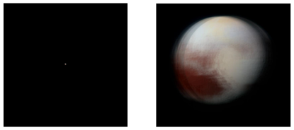
Figure S3: Pluto when imaged under the assumption that it has the same size as the moon and is placed at a distance such that its angular size is equal to the one of Jupiter ($\phi_{m}\approx 0.01^{\circ}$). The image was obtained with the $20D$ Totimorphic mirror configuration. As can be seen on the left, the image is much smaller due to the drastically increased distance of the object. Thus, even though the object is still recognizable, sharp details are lost due to the non-perfect focusing of the light (right).

In the second application, we demonstrated how a Totimorphic lattice can be used as the backbone for autonomously deployable and reconfigurable large-scale space infrastructure, specifically the primary mirror element of a telescope. A major criterion for the operability of such a mirror is how accurately it focuses the reflected light, as this directly limits the attainable resolution when imaging objects. For objects at far larger distances, e.g., with angular sizes similar to Jupiter, we can already see that the magnification of our design is not sufficient to produce sharp images – although rough details are still recognizable (see Fig. S3). This can be improved by further increasing the focal length. An approach that is often used in modern telescopes is to guide the light through a hierarchy of mirrors, e.g., by adding a secondary or even tertiary mirror before projecting the light onto a sensor. In our case, those mirrors would be Totimorphic as well. Due to the differentiability of the whole process, our framework can be used to (re)configure all mirrors simultaneously. This way, subsequent mirrors can even compensate for distortions introduced by previous (or later) mirrors. In addition, the focusing of a mirror based on a Totimorphic lattice can be improved by reducing the size of unit cells. The effect of miniaturisation on focal length and the physical properties of the Totimorphic cells must be quantified to mature this concept.

Developing a practical prototype of a Totimorphic structure will require overcoming many pressing technical challenges, as the underlying assumptions and abstractions used in the model become physically unrealistic. For instance, it is assumed that the beams and levers are perfectly rigid. In reality, deformations in the structure from external or internal forces will produce bending in the beams, destabilising the internal spring forces. Similarly, the zero-length property of the springs will likely not hold for a real structure. While it is possible to create springs that approximate the property for a range of lengths, at small or large extensions the zero-length property will likely not persist. Moreover, when in the zero-stiffness state, the Totimorphic structure should require no work to move between configurations, but practically there will be friction and jamming in the joints of the structure, which requires work from actuators to overcome. Independent of the application, minimising the number of actuators required to operate a spacecraft is quite critical, as each actuator represents a mode of failure that might compromise the spacecraft. Vacuum-exposed mechanisms and actuators are also at risk of cold welding and are difficult to lubricate. Since the number of actuators required to control a Totimorphic lattice scales linearly with the number of unit cells, it will be critical to investigate whether it is possible to reduce the number of actuators and optimise the operations required to morph between given configurations. The specifics of transforming 1D springs, Euler beams and frictionless joints into a manufacturable model is beyond the scope of this paper, but it will be necessary to make decisions that balance the requirements with suitability for space on various aspects like material choices, beam/lever aspect ratios, joint types, and actuation methods.

Despite the challenges, Totimorphic lattices have a number of advantages for use in space environment. Deployable, reconfigurable, low-density structures are highly desirable for the strict mass and energy requirements of most space missions. We suggest that Totimorphic structures potentially fill a functional gap between Origami and inflatable structures, being able to carry tensile and compressive loads while also being flexible and capable of supporting surfaces without requiring pressurisation. Totimorphic structures may be compatible with further applications – a variety of space infrastructure use-cases such as space antennas and solar sails.

To conclude, Totimorphic structures represent an intriguing class of mechanically reprogrammable systems, featuring continuously adjustable effective physical properties through simple mechanical actuations. Especially since our framework is light-weight and flexible regarding the cost function, it can be implemented on edge devices to allow autonomous and lattice-aware control of the actuators, e.g., using a deep neural network to estimate effective properties of the Totimorphic structure from the state of its actuators (the generalized coordinates). Thus, we are confident that the introduced concept can be scaled up to real-world, large-scale prototypes capable of autonomously and continuously adapting their lattice configuration to achieve a specified objective.

4 Methods

In the following, we describe the mathematical models referenced in the main text. These are just one particular realisation of an analytical Totimorphic model, and the introduced framework can be extended to other Totimorphic structures in a straightforward way. Implementations of the models in Python are available on Gitlab.

4.1 Notation

We first introduce the notation used in the following sections. Polar vectors are denoted by:

$$\boldsymbol{e}^{\alpha}=\begin{pmatrix}\cos{\alpha}\\ \sin{\alpha}\end{pmatrix}\,.$$ (5)

For proofs, we will be using the identity:

$$\boldsymbol{e}^{\alpha}\cdot\boldsymbol{e}^{\beta}=\text{cos}\left(\alpha-\beta\right)\,.$$ (6)

We also introduce the operator $E\left(\cdot\right):\mathbb{R}^{2}\to\mathbb{R}$ that returns the angles $\alpha$ required to represent a vector $\boldsymbol{r}$ in polar coordinates, given by:

$$\alpha=E\left(\boldsymbol{r}\right)=\text{sign}\left(r_{y}\right)\cdot\arccos{\left(\frac{r_{x}}{\|\boldsymbol{r}\|}\right)}\,.$$ (7)

Rotation matrices in three-dimensional Euclidean space are given by:

$$R_{x}(\alpha)=\begin{pmatrix}1&0&0\\ 0&\cos{\alpha}&-\sin{\alpha}\\ 0&\sin{\alpha}&\cos{\alpha}\end{pmatrix}\,,$$ (8)

$$R_{y}(\alpha)=\begin{pmatrix}\cos{\alpha}&0&\sin{\alpha}\\ 0&1&0\\ -\sin{\alpha}&0&\cos{\alpha}\end{pmatrix}\,,$$ (9)

$$R_{z}(\alpha)=\begin{pmatrix}\cos{\alpha}&-\sin{\alpha}&0\\ \sin{\alpha}&\cos{\alpha}&0\\ 0&0&1\end{pmatrix}\,.$$ (10)

Similarly, we denote the standard polar vector in three dimensions by:

$$\boldsymbol{\xi}^{\alpha,\beta}=\begin{pmatrix}\cos{\alpha}\sin{\beta}\\ \sin{\alpha}\sin{\beta}\\ \cos{\beta}\end{pmatrix}\,.$$ (11)

To gain the angles for representing a general vector $\boldsymbol{r}$ in these coordinates, we introduce $\Xi\left(\cdot\right):\mathbb{R}^{3}\to\mathbb{R}^{2}$ given by:

$$\begin{pmatrix}\alpha\\ \beta\end{pmatrix}=\Xi\left(\boldsymbol{r}\right)=\begin{pmatrix}\text{sign}\left(r_{y}\right)\cdot\arccos{\left(\frac{r_{x}}{\sqrt{r_{x}^{2}+r_{y}^{2}}}\right)}\\ \arccos\left(\frac{r_{z}}{\|\boldsymbol{r}\|}\right)\end{pmatrix}$$ (12)

We further use the following polar representation:

$$\boldsymbol{\epsilon}^{\alpha,\beta}=\begin{pmatrix}\cos{\alpha}\cos{\beta}\\ \sin{\beta}\\ -\sin{\alpha}\cos{\beta}\end{pmatrix}=R_{y}(\alpha)R_{z}(\beta)\mathbb{1}_{x}$$ (13)

with

$$\mathbb{1}_{x}=\begin{pmatrix}1\\ 0\\ 0\end{pmatrix}$$ (14)

To gain the angles for representing a general vector $\boldsymbol{r}$ in these coordinates, we introduce $\mathcal{E}\left(\cdot\right):\mathbb{R}^{3}\to\mathbb{R}^{2}$ given by:

$$\begin{pmatrix}\alpha\\ \beta\end{pmatrix}=\mathcal{E}\left(\boldsymbol{r}\right)=\begin{pmatrix}-\text{sign}\left(r_{z}\right)\cdot\arccos{\left(\frac{r_{x}}{\sqrt{r_{x}^{2}+r_{z}^{2}}}\right)}\\ \arcsin\left(\frac{r_{y}}{\|\boldsymbol{r}\|}\right)\end{pmatrix}$$ (15)

For proofs, the following identity is used:

$$\boldsymbol{\xi}^{\alpha,\beta}\cdot\boldsymbol{\xi}^{\phi,\Theta}=\cos\left(\alpha-\phi\right)\sin{\beta}\sin{\Theta}+\cos{\beta}\cos{\Theta}\,.$$ (16)

4.2 Totimorphic lattices in two dimensions

4.2.1 Parametrisation of elementary cells

In the following, we drop the index $ij$ (cell at row $i$ and column $j$) for clarity. However, all vectors are always given per elementary cell (see main text). An elementary cell is constructed from two unit cells which are connected at their levers. An elementary cell in the Totimorphic lattice is parameterized by $(\boldsymbol{o},\varphi,\theta,\varphi^{\prime},\theta^{\prime})$, where $\boldsymbol{o}$ is the location of point $A$, $\varphi$ is the angle with the x-axis of the lower beam, and $\theta$ is the angle of the lower lever with respect to the lower beam. Primed variables represent the same quantities, but for the upper half of the elementary cell (i.e., the upper beam and lever).

The points of the lower unit cell are given by:

$$\boldsymbol{r}^{\mathrm{A}} =\boldsymbol{o}\,,$$ (17a)

$$\boldsymbol{r}^{\mathrm{B}} =\boldsymbol{r}^{\mathrm{A}}+l_{\text{b}}\cdot\boldsymbol{e}^{\varphi}\,,$$ (17b)

$$\boldsymbol{r}^{\mathrm{P}} =\boldsymbol{r}^{\mathrm{A}}+\frac{l_{\text{b}}}{2}\cdot\boldsymbol{e}^{\varphi}\,,$$ (17c)

$$\boldsymbol{r}^{\mathrm{C}} =\boldsymbol{r}^{\mathrm{P}}+\frac{l_{\text{b}}}{2}\cdot\boldsymbol{e}^{\varphi+\theta}\,.$$ (17d)

The points of the upper unit cell are given by:

$$\boldsymbol{r}^{\mathrm{P^{\prime}}}=\boldsymbol{r}^{\mathrm{C}}+\frac{l_{\text{b}}}{2}\boldsymbol{e}^{\gamma^{\prime}} \ \ \ \ \text{with}\ \ \ \ \gamma^{\prime}=\pi-\theta^{\prime}+\varphi^{\prime}\,,$$ (18a)

$$\boldsymbol{r}^{\mathrm{A^{\prime}}} =\boldsymbol{r}^{\mathrm{P^{\prime}}}-\frac{l_{\text{b}}}{2}\cdot\boldsymbol{e}^{\varphi^{\prime}}\,,$$ (18b)

$$\boldsymbol{r}^{\mathrm{B^{\prime}}}=\boldsymbol{r}^{\mathrm{P^{\prime}}}+ \frac{l_{\text{b}}}{2}\cdot\boldsymbol{e}^{\varphi^{\prime}}=2\cdot\boldsymbol{r}^{\mathrm{P^{\prime}}}-\boldsymbol{r}^{\mathrm{A^{\prime}}}\,.$$ (18c)

For the upper triangle, we recover $\varphi^{\prime}$ via

$$\boldsymbol{e}^{\varphi^{\prime}} =\frac{1}{l_{\text{b}}}\cdot\left(\boldsymbol{r}^{\mathrm{B^{\prime}}}-\boldsymbol{r}^{\mathrm{A^{\prime}}}\right)\,,$$ (19a)

$$\varphi^{\prime} =\text{sign}\left(e^{\varphi^{\prime}}_{y}\right)\cdot\text{arccos}\left(e^{\varphi^{\prime}}_{x}\right)\,,$$ (19b)

and $\theta^{\prime}$ through

$$\boldsymbol{e}^{\gamma^{\prime}} =\frac{2}{l_{\text{b}}}\cdot\left(\boldsymbol{r}^{\mathrm{P^{\prime}}}-\boldsymbol{r}^{\mathrm{C}}\right)\,,$$ (20a)

$$\gamma^{\prime} =\text{sign}\left(e^{\gamma^{\prime}}_{y}\right)\cdot\text{arccos}\left(e^{\gamma^{\prime}}_{x}\right)\,,$$ (20b)

$$\theta^{\prime} =\pi-\gamma^{\prime}+\varphi^{\prime}\,,$$ (20c)

with $\varphi^{\prime}$ given by Eq. 19b.

To check for overlapping springs in the elementary cell, representing a state in which the cell physically breaks, we introduce the following angles per elementary cell:

$$\alpha^{\prime}_{\mathrm{L}}{} =\frac{\theta^{\prime}}{2}-\varphi^{\prime}\,,$$ (21a)

$$\alpha^{\prime}_{\mathrm{R}}{} =\frac{\pi}{2}-\alpha^{\prime}_{\mathrm{L}}{}\,,$$ (21b)

$$\alpha_{\mathrm{L}}{} =\frac{\theta}{2}+\varphi\,,$$ (21c)

$$\alpha_{\mathrm{R}}{} =\frac{\pi}{2}-\alpha_{\mathrm{L}}{}\,.$$ (21d)

$\alpha_{\mathrm{L}}{}$ is the angle of the bottom left spring (connecting points $A$ and $C$) with the x-axis, while $\alpha_{\mathrm{R}}{}$ is the angle of the bottom right spring (connecting points $B$ and $C$). Primed angles indicate the same for the top unit cell. Angles are measured with respect to the x-axis going through point $C$, hence in the flat configuration, top angles are negative and bottom angles are positive.

4.2.2 Connecting elementary cells

The first elementary cell ($i=0$, $j=0$) can be constructed freely, as there are no other cells to connect it to. Adding more unit cells horizontally ($i=0$, $j>0$) is done iteratively as follows. First, we enforce the constraint of connecting the two elementary cells:

$$\boldsymbol{r}^{\mathrm{A}}_{0j} =\boldsymbol{r}^{\mathrm{B}}_{0j-1}\,,$$ (22a)

$$\boldsymbol{r}^{\mathrm{A^{\prime}}}_{0j} =\boldsymbol{r}^{\mathrm{B^{\prime}}}_{0j-1}\,.$$ (22b)

Then we have to obtain the point $P^{\prime}$ of our new elementary cell, which has to satisfy the Totimorphic condition. In the following, all points are in the same elementary cell $(0j)$, and thus we drop the indices for convenience. The condition for the existence of $\boldsymbol{r}^{\mathrm{P^{\prime}}}$ is that lever and beam with fixed length have to connect to it from point $A^{\prime}$ (given by the first elementary cell) and point $C$:

$$\|\boldsymbol{r}^{\mathrm{A^{\prime}}}-\boldsymbol{r}^{\mathrm{P^{\prime}}}\|^{2} =\left(\frac{l_{\text{b}}}{2}\right)^{2}\,,$$ (23a)

$$\|\boldsymbol{r}^{\mathrm{C}}-\boldsymbol{r}^{\mathrm{P^{\prime}}}\|^{2} =\left(\frac{l_{\text{b}}}{2}\right)^{2}\,.$$ (23b)

Introducing $\boldsymbol{s}^{-}=\boldsymbol{r}^{\mathrm{A^{\prime}}}-\boldsymbol{r}^{\mathrm{C}}$, $\boldsymbol{s}^{+}=\boldsymbol{r}^{\mathrm{A^{\prime}}}+\boldsymbol{r}^{\mathrm{C}}$ and $\delta=\frac{1}{2}\left(\|\boldsymbol{r}^{\mathrm{A^{\prime}}}\|^{2}-\|\boldsymbol{r}^{\mathrm{C}}\|^{2}\right)$, we get

$$r^{\mathrm{P^{\prime}}}_{x} =\frac{\delta-r^{\mathrm{P^{\prime}}}_{y}s^{-}_{y}}{s^{-}_{x}}\,,$$ (24)

$$r^{\mathrm{P^{\prime}}}_{y} =\frac{1}{2}\left(s^{+}_{y}-s^{-}_{x}\sqrt{\left(\frac{l_{\text{b}}}{\|\boldsymbol{s}^{-}\|}\right)^{2}-1}\right)\,.$$ (25)

A detailed derivation can be found in the supplemental information.

4.2.3 Conditions for intact elementary cells

The criteria for being intact are the same for every unit cell $(ij)$, therefore indices are dropped again in the following to ease notation. An elementary cell is considered intact if the following conditions are met:

$$\|\boldsymbol{s}^{-}\ \| \leq l_{\text{b}}\,,$$ (26)

$$\alpha^{\prime}_{\mathrm{L}}{}+\alpha_{\mathrm{L}}{} \geq 0\,,$$ (27)

$$\alpha^{\prime}_{\mathrm{R}}{}+\alpha_{\mathrm{R}}{} \geq 0\,.$$ (28)

The first condition means that springs cannot be stretched further than the beam length. The second (third) conditions check whether the left (right) bottom and top springs cross.

To avoid overstretched springs, we correct $\theta$ by constraining its range. The limits of this interval are obtained by the criterion for the existence of real-values solutions of Eq. 25 (the term below the root has to be $\geq 0$, see supplemental information):

$$\Delta-\arccos{\left(C\right)}\leq\theta\leq\Delta+\arccos{\left(C\right)}\,.$$ (29)

with $\boldsymbol{k}=\boldsymbol{r}^{\mathrm{A^{\prime}}}-\boldsymbol{r}^{\mathrm{A}}-\frac{l_{\text{b}}}{2}\boldsymbol{e}^{\varphi}$, $\Phi=E\left(\boldsymbol{k}\right)$, $\Delta=\Phi-\varphi$, and $C=\frac{\|\boldsymbol{k}\|}{l_{\text{b}}}-\frac{3}{4}\frac{l_{\text{b}}}{\|\boldsymbol{k}\|}$. If the interval for $\theta$ is empty, it is impossible to add a new elementary cell without changing the configuration of previous cells in the structure. These conditions are checked for each unit cell separately while constructing it.

4.2.4 Building a structure

For $i>0$ and $j=0$, one sets $\varphi_{i0}=\varphi^{\prime}_{i-1,0}$, $\boldsymbol{r}^{\mathrm{A}}_{i,0}=\boldsymbol{r}^{\mathrm{A^{\prime}}}_{i-1,0}$, and calculates all points as for the first elementary cell ($i=0$, $j=0$). In all remaining cases, we set $\varphi_{ij}=\varphi^{\prime}_{i-1,j}$, $\boldsymbol{r}^{\mathrm{A}}_{i,j}=\boldsymbol{r}^{\mathrm{B}}_{i,j-1}$, $\boldsymbol{r}^{\mathrm{A^{\prime}}}_{ij}=\boldsymbol{r}^{\mathrm{B^{\prime}}}_{i,j-1}$, and calculate the remaining points by solving for $\mathrm{P^{\prime}}$.

Depending on where in the lattice an elementary cell is positioned, it is characterised by the following parameters:

1. $i=0$, $j=0$: $(\boldsymbol{o}_{00},\varphi_{00},\theta_{00},\varphi^{\prime}_{00},\theta^{\prime}_{00})$  ,

2. $i=0$, $j>0$: $(\varphi_{0j},\theta_{0j})$  ,

3. $i>0$, $j=0$: $(\theta_{i0},\varphi^{\prime}_{i0},\theta^{\prime}_{i0})$  ,

4. else: $(\theta_{ij})$  .

To initialise the lattice as a flat surface, beam angles $\varphi_{ij}$ and $\varphi^{\prime}_{ij}$ have to be set to $0$ and lever angles $\theta_{ij}$ and $\theta^{\prime}_{ij}$ to $\frac{\pi}{2}$ $\forall i,j$.

4.3 Totimorphic lattices in three dimensions

4.3.1 Parametrisation of elementary cells

As in the two-dimensional case, each elementary cell is characterised by the angles of the beams and levers, $(\boldsymbol{o},\varphi_{y}{},\varphi_{z}{},\theta_{x}{},\theta_{z}{},\varphi^{\prime}_{y}{},\varphi^{\prime}_{z}{},\theta^{\prime}_{x}{},\theta^{\prime}_{z}{})$.

The points of the lower unit cell are given by:

$$\boldsymbol{r}^{\mathrm{A}} =\boldsymbol{o}\,,$$ (30a)

$$\boldsymbol{r}^{\mathrm{B}} =\boldsymbol{r}^{\mathrm{A}}+l_{\text{b}}\cdot\boldsymbol{\epsilon}^{\varphi_{y},\varphi_{z}}\,,$$ (30b)

$$\boldsymbol{r}^{\mathrm{P}} =\boldsymbol{r}^{\mathrm{A}}+\frac{l_{\text{b}}}{2}\cdot\boldsymbol{\epsilon}^{\varphi_{y},\varphi_{z}}\,,$$ (30c)

$$\boldsymbol{r}^{\mathrm{C}} =\boldsymbol{r}^{\mathrm{P}}+\frac{l_{\text{b}}}{2}\cdot R_{y}(\varphi_{y})R_{z}(\varphi_{z})R_{x}(\theta_{x})R_{z}(\theta_{z})\mathbb{1}_{x}\,.$$ (30d)

Here, the beam is described by its rotation in the x-y plane (given by $\varphi_{z}{}$, which corresponds to $\varphi$ in the two-dimensional case) and a rotation in x-z plane (a tilting of the unit cell given by $\varphi_{y}$). The orientation of the lever is obtained by a sequence of rotations: first, we rotate the x-direction unit vector $\mathbb{1}_{x}$ by $\theta_{z}$ (in the two-dimensional case, we called this $\theta$), then tilt it in the y-z plane by $\theta_{x}$, and then apply the same transformation (two rotations) used to gain the beam vector from the unit vector. We choose this parametrisation so that the angles of the lever are again defined with respect to the orientation of the beam, as in the two-dimensional case.

The points of the upper unit cell are defined similarly:

$$\boldsymbol{r}^{\mathrm{P^{\prime}}} =\boldsymbol{r}^{\mathrm{C}}+\frac{l_{\text{b}}}{2}\cdot R_{y}(\varphi^{\prime}_{y})R_{z}(\varphi^{\prime}_{z})R_{x}(-\theta^{\prime}_{x})R_{z}(-\theta^{\prime}_{z})\mathbb{1}_{x}\,,$$ (31a)

$$\boldsymbol{r}^{\mathrm{A^{\prime}}} =\boldsymbol{r}^{\mathrm{P^{\prime}}}-\frac{l_{\text{b}}}{2}\cdot\boldsymbol{\epsilon}^{\varphi^{\prime}_{y},\varphi^{\prime}_{z}}\,,$$ (31b)

$$\boldsymbol{r}^{\mathrm{B^{\prime}}} =\boldsymbol{r}^{\mathrm{P^{\prime}}}+\frac{l_{\text{b}}}{2}\cdot\boldsymbol{\epsilon}^{\varphi^{\prime}_{y},\varphi^{\prime}_{z}}\,.$$ (31c)

4.3.2 Connecting elementary cells

Again, the first elementary cell ($i=0$, $j=0$) is unconstrained and can be constructed freely. Without loss of generality, we initialise lattices lying in the x-z plane. Adding more unit cells horizontally ($i=0$, $j>0$) is done iteratively as follows. First, we enforce the constraint of connecting the two elementary cells:

$$\boldsymbol{r}^{\mathrm{A}}_{0j} =\boldsymbol{r}^{\mathrm{B}}_{0j-1}\,,$$ (32a)

$$\boldsymbol{r}^{\mathrm{A^{\prime}}}_{0j} =\boldsymbol{r}^{\mathrm{B^{\prime}}}_{0j-1}\,.$$ (32b)

In the following, all points are in the same elementary cell $(0j)$, and thus we drop the indices for convenience. As in the two-dimensional case, we look again for a consistent solution for $\boldsymbol{r}^{\mathrm{P^{\prime}}}$. The vector representing the upper beam is given by $l_{\text{b}}\cdot\boldsymbol{\xi}^{\phi,\Theta}$ (the traditional angles are recovered via $(\varphi_{y}{},\varphi_{z}{})=\mathcal{E}\left(\boldsymbol{\xi}^{\phi,\Theta}\right)$. The lever is then given by the vector

$$\boldsymbol{r}_{L} =\boldsymbol{r}^{\mathrm{A^{\prime}}}-\boldsymbol{r}^{\mathrm{C}}+\frac{l_{\text{b}}}{2}\boldsymbol{\xi}^{\phi,\Theta}\,,$$ (33a)

$$=\boldsymbol{s}^{-}+\frac{l_{\text{b}}}{2}\cdot\boldsymbol{\xi}^{\phi,\Theta}\,.$$ (33b)

For $P^{\prime}$ to exist, the lever has to have the correct length:

$$\|\boldsymbol{r}_{L}\|^{2}=\frac{l_{\text{b}}}{2}^{2}\,.$$ (34)

From this, we obtain a solution for $\phi$ and $\Theta$, with $\phi$ being completely determined by $\Theta$. Additionally, as in the two-dimensional case, we gain valid intervals for both $\Theta$ as well as $\theta_{z}$. The remaining points are then given by:

$$\boldsymbol{r}^{\mathrm{P^{\prime}}}=\boldsymbol{r}^{\mathrm{A^{\prime}}}+\frac{l_{\text{b}}}{2}\cdot\boldsymbol{\xi}^{\phi,\Theta}\,,$$ (35a)

$$\boldsymbol{r}^{\mathrm{B^{\prime}}}=\boldsymbol{r}^{\mathrm{A^{\prime}}}+l_{\text{b}}\cdot\boldsymbol{\xi}^{\phi,\Theta}\,.$$ (35b)

A detailed derivation of the angles and their constrained intervals can be found in the supplemental information.

4.3.3 Building a structure

For $i>0$ and $j=0$, one sets $\varphi_{z;i0}=\varphi^{\prime}_{z;i-1,0}$, $\varphi_{y;i0}=\varphi^{\prime}_{y;i-1,0}$, $\boldsymbol{r}^{\mathrm{A}}_{i,0}=\boldsymbol{r}^{\mathrm{A^{\prime}}}_{i-1,0}$, and calculates all points as for the first unit cell ($i=0$, $j=0$). In all remaining cases, we set $\varphi_{z;i0}=\varphi^{\prime}_{z;i-1,0}$, $\varphi_{y;i0}=\varphi^{\prime}_{y;i-1,0}$, $\boldsymbol{r}^{\mathrm{A}}_{i,j}=\boldsymbol{r}^{\mathrm{B}}_{i,j-1}$, $\boldsymbol{r}^{\mathrm{A^{\prime}}}_{ij}=\boldsymbol{r}^{\mathrm{B^{\prime}}}_{i,j-1}$, and calculate the remaining points by solving for $\phi$ and $\Theta$.

Depending on where in the lattice an elementary cell is positioned, it is characterised by the following parameters:

1. $i=0$, $j=0$: $(\boldsymbol{o},\varphi_{y}{},\varphi_{z}{},\theta_{x}{},\theta_{z}{},\varphi^{\prime}_{y}{},\varphi^{\prime}_{z}{},\theta^{\prime}_{x}{},\theta^{\prime}_{z}{})$

2. $i=0$, $j>0$: $(\varphi_{y}{},\varphi_{z}{},\theta_{x}{},\theta_{z}{},\Theta)$

3. $i>0$, $j=0$: $(\theta_{x}{},\theta_{z}{},\varphi^{\prime}_{y}{},\varphi^{\prime}_{z}{},\theta^{\prime}_{x}{},\theta^{\prime}_{z}{})$

4. else: $(\theta_{x}{},\theta_{z}{},\Theta)$

To initialise the lattice as a flat surface in x-z plane, beam angles $\varphi_{z;ij}$ and $\varphi^{\prime}_{z;ij}$ have to be set to $\frac{\pi}{2}$ and all remaining angles to 0.

4.4 Direct Stiffness method

The fundamental building block of the direct stiffness method is rod or beam-like elements characterised by the coordinates of its two ending points $i,j\in\mathbb{N}$, i.e., $(x_{i},y_{i})$ and $(x_{j},y_{j})$. Applying forces $(\boldsymbol{F}_{i},\boldsymbol{F}_{j})$ to the two ending points of the element results in a deformation of the element; or more specifically, a displacement of the ending points $(\boldsymbol{u}_{i},\boldsymbol{u}_{j})$, which is calculated from the stiffness equation (a generalisation of Hook’s law):

$$\boldsymbol{K}_{ij}\begin{pmatrix}\boldsymbol{u}_{i}\\ \boldsymbol{u}_{j}\end{pmatrix}=\begin{pmatrix}\boldsymbol{F}_{i}\\ \boldsymbol{F}_{j}\end{pmatrix}\,,$$ (36)

with $\boldsymbol{K}_{ij}$ being the stiffness matrix, and $\boldsymbol{u}_{i}=(u^{x}_{i},u^{y}_{i},u^{\varphi}_{i})$ being the resulting displacements due to external forces and moments $\boldsymbol{F}_{i}=(F^{x}_{i},F^{y}_{i},M^{\varphi}_{i})$. $\varphi$ characterises the resulting bending of beam elements. Thus, the updated equilibrium state of the beam after applying forces is given by $(x_{i}+u^{x}_{i},y_{i}+u^{y}_{i})$ and $(x_{j}+u^{x}_{j},y_{j}+u^{y}_{j})$. Repeating this process by recalculating the stiffness matrix using the updated coordinates and solving Eq. 36 anew, deformations due to larger forces can be obtained.

4.4.1 Generalized Euler-Bernoulli beam elements

In this work, we use generalized Euler-Bernoulli beam elements to model the beams and levers in a Totimorphic lattice. The stiffness matrix $\boldsymbol{K}_{ij}$ of the generalized beam element is obtained by combining the stiffness matrices of rod elements, i.e., elements that behave like springs,

$$\boldsymbol{K}^{\mathrm{rod}}_{ij}=\frac{E_{ij}A_{ij}}{L_{ij}}\begin{pmatrix}c_{ij}^{2}&c_{ij}s_{ij}&0&-c_{ij}^{2}&-c_{ij}s_{ij}&0\\ c_{ij}s_{ij}&s_{ij}^{2}&0&-c_{ij}s_{ij}&-s_{ij}^{2}&0\\ 0&0&0&0&0&0\\ -c_{ij}^{2}&-c_{ij}s_{ij}&0&c_{ij}^{2}&c_{ij}s_{ij}&0\\ -c_{ij}s_{ij}&-s_{ij}^{2}&0&c_{ij}s_{ij}&s_{ij}^{2}&0\\ 0&0&0&0&0&0\end{pmatrix}\,.$$ (37)

and Euler-Bernoulli beam elements that model bending [31]

$$\boldsymbol{K}^{\mathrm{EB}}_{ij}=\frac{E_{ij}I_{ij}}{L_{ij}^{3}}\cdot\begin{pmatrix}12s_{ij}^{2}&-12s_{ij}c_{ij}&-6L_{ij}s_{ij}&-12s_{ij}^{2}&12s_{ij}c_{ij}&-6L_{ij}s_{ij}\\ -12s_{ij}c_{ij}&12c_{ij}^{2}&6L_{ij}c_{ij}&12s_{ij}c_{ij}&-12c_{ij}^{2}&6L_{ij}c_{ij}\\ -6L_{ij}s_{ij}&6L_{ij}c_{ij}&4L_{ij}^{2}&6L_{ij}s_{ij}&-6L_{ij}c_{ij}&2L_{ij}^{2}\\ -12s_{ij}^{2}&12s_{ij}c_{ij}&6L_{ij}s_{ij}&12s_{ij}^{2}&-12s_{ij}c_{ij}&6L_{ij}s_{ij}\\ 12s_{ij}c_{ij}&-12c_{ij}^{2}&-6L_{ij}c_{ij}&-12s_{ij}c_{ij}&12c_{ij}^{2}&-6L_{ij}c_{ij}\\ -6L_{ij}s_{ij}&6L_{ij}c_{ij}&2L_{ij}^{2}&6L_{ij}s_{ij}&-6L_{ij}c_{ij}&4L_{ij}^{2}\end{pmatrix}\,,$$ (38)

resulting in

$$\boldsymbol{K}_{ij}=\boldsymbol{K}^{\mathrm{rod}}_{ij}+\boldsymbol{K}^{\mathrm{EB}}_{ij}\,.$$ (39)

Here, $L_{ij}$ is the length of the beam, and $s_{ij}$ and $c_{ij}$ are the sine and cosine of the angle $\vartheta_{ij}$ of the beam with respect to the x-axis:

$$L_{ij} =\sqrt{(x_{j}-x_{i})^{2}+(y_{j}-y_{i})^{2}}\,,$$ (40)

$$c_{ij} =\cos\left(\vartheta_{ij}\right)\,,$$ (41)

$$s_{ij} =\sin\left(\vartheta_{ij}\right)\,.$$ (42)

$E_{ij}$, $A_{ij}$, and $I_{ij}$ are the elements Young’s modulus, cross-sectional area, and second moment of area, respectively. For simplicity, we choose a uniform lattice with $E_{ij}=E$, $I_{ij}=I$, and $A_{ij}=A$.

4.4.2 Compression experiment

The global stiffness matrix $\boldsymbol{G}$ of a whole lattice structure is obtained by adding up the stiffness matrices of the individual beams and levers accordingly. The stiffness equation for the whole structure then takes the same form as the one for individual elements, but it contains all lattice point coordinates (ending points of Totimorphic beams or levers, i.e., points $A$, $A^{\prime}$, $B$, $B^{\prime}$, $P$, $P^{\prime}$, and $C$ of each elementary cell):

$$\boldsymbol{G}\begin{pmatrix}\boldsymbol{u}_{0}\\ \boldsymbol{u}_{1}\\ ...\\ \boldsymbol{u}_{N-1}\end{pmatrix}=\begin{pmatrix}\boldsymbol{F}_{0}\\ \boldsymbol{F}_{1}\\ ...\\ \boldsymbol{F}_{N-1}\end{pmatrix}\,.$$ (43)

To implement the compression experiment, we first set the displacement of points that are part of the top surface of the lattice to a small non-zero value. As boundary conditions, we set the displacement of all points in the bottom surface to zero (otherwise, the lattice would start moving downwards). Using Eq. 43 (i.e. matrix multiplication), we calculate the resulting forces for all other points due to these forced displacements – from which we subsequently calculate the resulting displacements of all remaining points in the lattice that are not part of the top or bottom surface by solving a system of linear equations. We repeat this process several times (with updated global stiffness matrix $\boldsymbol{G}$) to obtain macroscopic deformations. For a detailed description, see [9].

4.4.3 Poisson’s ratio

Assume we do $k$ iterations in the compression experiment, i.e., we solve Eq. 43 $k$ times in sequence, and in each iteration we displace the top lattice points by $\epsilon_{k}$. After each iteration, we collect the displacement in $x$-direction of the outer left and outer right points of the lattice, calculate the mean displacement over these points, and then obtain the average change in width of the lattice by taking the difference:

$$\Delta R_{k} =\frac{1}{|\mathcal{RS}|}\sum_{i\in\mathcal{RS}}u^{x}_{i,k}\,,$$ (44)

$$\Delta L_{k} =\frac{1}{|\mathcal{LS}|}\sum_{i\in\mathcal{LS}}u^{x}_{i,k}\,,$$ (45)

$$\bar{\epsilon}_{k} =\Delta R_{k}-\Delta L_{k}\,,$$ (46)

where $\mathcal{LS}$ ($\mathcal{RS}$) is a set containing the indices of the points on the left (right) surface of the lattice. $|\mathcal{RS}|$ denotes the number of elements in $\mathcal{RS}$. The Poisson’s ratio is obtained using linear regression

$$\nu=\frac{\sum_{k}\bar{\epsilon}_{k}}{\sum_{k}\epsilon_{k}}\,.$$ (47)

4.5 Ray-based optics

In the telescope mirror application (Section 2.4), for simplicity, we only simulate light rays getting reflected at the mid-point (i.e. the mid-point of the lever) of each unit cell. Thus, each unit cell acts as a tiny mirror reflecting a single beam of light. We assume light coming from a source that is far away, such that the light rays hitting the different mirror elements are parallel to each other.

4.5.1 Reflections

To calculate the light reflection, we have to know the orientation of the surface of reflection, which is given by the normal vector of each unit cell. For a single elementary cell, the normal vectors of its two unit cells are

$$\boldsymbol{n}_{ij} =\frac{\left(\boldsymbol{r}^{\mathrm{B}}_{ij}-\boldsymbol{r}^{\mathrm{A}}_{ij}\right)\times\left(\boldsymbol{r}^{\mathrm{C}}_{ij}-\boldsymbol{r}^{\mathrm{A}}_{ij}\right)}{\|\left(\boldsymbol{r}^{\mathrm{B}}_{ij}-\boldsymbol{r}^{\mathrm{A}}_{ij}\right)\times\left(\boldsymbol{r}^{\mathrm{C}}_{ij}-\boldsymbol{r}^{\mathrm{A}}_{ij}\right)\|_{2}}\,,$$ (48)

$$\boldsymbol{n}^{\prime}_{ij} =\frac{\left(\boldsymbol{r}^{\mathrm{B^{\prime}}}_{ij}-\boldsymbol{r}^{\mathrm{C}}_{ij}\right)\times\left(\boldsymbol{r}^{\mathrm{P^{\prime}}}_{ij}-\boldsymbol{r}^{\mathrm{C}}_{ij}\right)}{\|\left(\boldsymbol{r}^{\mathrm{B^{\prime}}}_{ij}-\boldsymbol{r}^{\mathrm{C}}_{ij}\right)\times\left(\boldsymbol{r}^{\mathrm{P^{\prime}}}_{ij}-\boldsymbol{r}^{\mathrm{C}}_{ij}\right)\|_{2}}\,,$$ (49)

where $\|\cdot\|_{2}$ is the Euclidean norm, $\times$ the vector cross product, and the primed vector denotes the top unit cell. The mid-points of the levers where the light is reflected are

$$\boldsymbol{m}_{ij} =\frac{1}{2}\left(\boldsymbol{r}^{\mathrm{P}}_{ij}+\boldsymbol{r}^{\mathrm{C}}_{ij}\right)\,,$$ (50)

$$\boldsymbol{m}^{\prime}_{ij} =\frac{1}{2}\left(\boldsymbol{r}^{\mathrm{P^{\prime}}}_{ij}+\boldsymbol{r}^{\mathrm{C}}_{ij}\right)\,.$$ (51)

Given a light ray with incidence direction $\boldsymbol{I}$ ($\|\boldsymbol{I}\|_{2}=1$), the directions of the reflected light $\boldsymbol{l}_{ij}$ coming from elementary cell $(ij)$ are given by

$$\boldsymbol{l}_{ij} =\frac{\boldsymbol{I}-2\left(\boldsymbol{I}\cdot\boldsymbol{n}_{ij}\right)\boldsymbol{n}_{ij}}{\|\boldsymbol{I}-2\left(\boldsymbol{I}\cdot\boldsymbol{n}_{ij}\right)\boldsymbol{n}_{ij}\|_{2}}\,,$$ (52)

$$\boldsymbol{l}^{\prime}_{ij} =\frac{\boldsymbol{I}-2\left(\boldsymbol{I}\cdot\boldsymbol{n}^{\prime}_{ij}\right)\boldsymbol{n}^{\prime}_{ij}}{\|\boldsymbol{I}-2\left(\boldsymbol{I}\cdot\boldsymbol{n}^{\prime}_{ij}\right)\boldsymbol{n}^{\prime}_{ij}\|_{2}}\,,$$ (53)

where $\cdot$ is the vector dot product.

4.5.2 Smallest distance to the target focal point

Given a target focal point $\boldsymbol{f}^{\mathrm{tgt}}$, we calculate the closest point $\boldsymbol{c}_{ij}$ ($\boldsymbol{c}^{\prime}_{ij}$) along the reflected ray to it as follows:

$$\boldsymbol{c}_{ij} =\boldsymbol{m}_{ij}+\big{(}(\boldsymbol{f}^{\mathrm{tgt}}-\boldsymbol{m}_{ij})\cdot\boldsymbol{l}_{ij}\big{)}\boldsymbol{l}_{ij}\,,$$ (54)

$$\boldsymbol{c}^{\prime}_{ij} =\boldsymbol{m}^{\prime}_{ij}+\big{(}(\boldsymbol{f}^{\mathrm{tgt}}-\boldsymbol{m}^{\prime}_{ij})\cdot\boldsymbol{l}^{\prime}_{ij}\big{)}\boldsymbol{l}^{\prime}_{ij}\,.$$ (55)

We then calculate the following cost function

$$C(\mathcal{P},\boldsymbol{f}^{\mathrm{tgt}})=\frac{1}{2N\cdot M}\sum_{i}^{N}\sum_{j}^{M}\big{(}\|\boldsymbol{c}_{ij}-\boldsymbol{f}^{\mathrm{tgt}}\|^{2}+\|\boldsymbol{c}^{\prime}_{ij}-\boldsymbol{f}^{\mathrm{tgt}}\|^{2}\big{)}\,,$$ (56)

and optimise the Totimorphic lattice by updating its parameters via gradient descent $\nabla_{\mathcal{P}}C(\mathcal{P},\boldsymbol{f}^{\mathrm{tgt}})$.

4.5.3 Damaging mirror elements

To emulate a damaged mirror element, we add a random perturbation to the direction of the reflected light. For instance, assuming the bottom unit cell of element $(ij)$ was damaged, we first sample a random deflection $\boldsymbol{l}_{\sigma}\sim\mathcal{N}(0,\sigma^{2})$ from a Gaussian distribution (with mean $0$ and variance $\sigma^{2}$) and always add it to the reflected light direction:

$$\boldsymbol{l}_{ij}\mapsto\frac{\boldsymbol{l}_{ij}+\boldsymbol{l}_{\sigma}}{\|\boldsymbol{l}_{ij}+\boldsymbol{l}_{\sigma}\|_{2}}\,.$$ (57)

For a single experiment, $\boldsymbol{l}_{\sigma}$ is only sampled once and kept constant afterwards.

4.5.4 Imaging

For imaging, we assume a picture of Pluto with the same diameter and distance as the Moon (radius of $r_{m}\approx 1700\cdot 10^{3}\,\mathrm{m}$ and angular radius of $\phi_{m}\approx 0.25^{\circ}$) has been placed at the same distance as the Moon (given by $d_{m}=r_{m}/\arctan\phi_{m}$).

For a $2S\times 2S$ pixel image of Pluto, the light ray coming from the pixel in row $i$ and column $j$ (counted from the bottom left corner of the image) has the an unnormalized incidence vector

$$\tilde{\boldsymbol{I}}_{ij}=\begin{pmatrix}\left(\frac{i}{S}-1\right)r_{m}\\ \left(\frac{j}{S}-1\right)r_{m}\\ -d_{m}\end{pmatrix}\,,$$ (58)

and the normalized one $\boldsymbol{I}_{ij}=\frac{\tilde{\boldsymbol{I}}_{ij}}{\|\tilde{\boldsymbol{I}}_{ij}\|_{2}}$. To get an image, we reflect the light rays coming from every pixel in the image at every Totimorphic mirror element and check where on the imaging plane the reflections hit. For instance, if the imaging plane is at distance $d_{z}$, the light ray $\boldsymbol{I}_{kl}$ reflected at the bottom unit cell of element $(ij)$ hits the plane at $\boldsymbol{m}_{ij}+\lambda\cdot\boldsymbol{l}_{ij}$ with $\lambda=\left(d_{z}-m_{ij,z}\right)/l_{ij,z}$ ($z$ denoting the $z$-component of the vectors). For visualisation, we plot all reflected points in a two-dimensional image with point size $s=2$ (in matplotlib) and an alpha (opacity) of $0.05$, so that colours merge when multiple points overlap.

Contributions

Initial idea is by AT and DD. Theory and model implementation is by DD, based on initial work by AT. All authors contributed to the design of the study and the performed experiments. DD and NR implemented code for the proof of concept experiments. DD wrote the first draft of the paper. All authors read and reviewed the final paper.

Supplemental Information

S1 Proofs for two-dimensional case

S1.1 Finding $\mathrm{P^{\prime}}$

In the following, we do not write the indices $ij$ explicitly to simplify the notation.

First, we start from the condition that $\mathrm{P^{\prime}}$ has to be chosen such that the resulting beam (connecting $\mathrm{A^{\prime}}$ and $\mathrm{P^{\prime}}$) and lever (connecting $\mathrm{C}$ and $\mathrm{P^{\prime}}$) have the desired length:

$$\|\boldsymbol{r}^{\mathrm{A^{\prime}}}-\boldsymbol{r}^{\mathrm{P^{\prime}}}\|^{2} =\left(\frac{l_{\text{b}}}{2}\right)^{2}\,,$$ (S1a)

$$\|\boldsymbol{r}^{\mathrm{C}}-\boldsymbol{r}^{\mathrm{P^{\prime}}}\|^{2} =\left(\frac{l_{\text{b}}}{2}\right)^{2}\,.$$ (S1b)

Expanding both expressions, subtracting Eq. S1b from Eq. S1a and dividing the resulting equation by $2$, we obtain:

$$\frac{1}{2}\left(\|\boldsymbol{r}^{\mathrm{A^{\prime}}}\|^{2}-\|\boldsymbol{r}^{\mathrm{C}}\|^{2}\right)-r^{\mathrm{P^{\prime}}}_{y}\left(r^{\mathrm{A^{\prime}}}_{y}-r^{\mathrm{C}}_{y}\right)-r^{\mathrm{P^{\prime}}}_{x}\left(r^{\mathrm{A^{\prime}}}_{x}-r^{\mathrm{C}}_{x}\right)=0\,.$$ (S2)

Using the notation $\boldsymbol{s}^{-}=\boldsymbol{r}^{\mathrm{A^{\prime}}}-\boldsymbol{r}^{\mathrm{C}}$, $\boldsymbol{s}^{+}=\boldsymbol{r}^{\mathrm{A^{\prime}}}+\boldsymbol{r}^{\mathrm{C}}$ and $\delta=\frac{1}{2}\left(\|\boldsymbol{r}^{\mathrm{A^{\prime}}}\|^{2}-\|\boldsymbol{r}^{\mathrm{C}}\|^{2}\right)$ as in the main text, this yields Eq. 24. Eq. 25 is then obtained by inserting this solution into either Eq. S1a or Eq. S1b and solving for $r^{\mathrm{P^{\prime}}}_{y}$. This results in a quadratic equation, possessing two solutions

$$r^{\mathrm{P^{\prime}}}_{y}=\frac{1}{2}\left(s^{+}_{y}\pm s^{-}_{x}\sqrt{\left(\frac{l_{\text{b}}}{\|\boldsymbol{s}^{-}\|}\right)^{2}-1}\right)\,.$$ (S3)

$\frac{1}{2}\boldsymbol{s}^{+}$ is the mid-point of the spring connecting point $C$ and $A^{\prime}$. Hence, $s^{+}_{y}$ is its $y$ coordinate (or height). If point $A^{\prime}$ is left of point $C$, as e.g. in the initial flat configuration, point $P^{\prime}$ has to be above this spring; meaning that its $y$ coordinate has to be larger than $s^{+}_{y}$. Since $s^{-}_{x}$ is negative in this scenario, the minus sign has to be chosen to get the correct solution. Similarly, if we pivot the unit cell such that $s^{-}_{x}=0$, i.e., $A^{\prime}$ and $C$ lie above each other, we have that $r^{\mathrm{P^{\prime}}}_{y}=\frac{1}{2}s^{+}_{y}$. Pivoting further, $P^{\prime}$ is situated below the spring (although it never swapped sides), as given by Eq. 25. Thus, when starting from the flat hour-glass motive, we have to choose the negative sign to get the correct solution for $P^{\prime}$.

S1.2 Condition for existing solution

For a solution of $\boldsymbol{r}^{\mathrm{P^{\prime}}}$ to exist, Eq. 25 has to be a real number, meaning that the argument of the square root has to be larger or equal to zero. This immediately yields Eq. 26.

S1.3 Deriving allowed range for $\theta$

First, we write out $\boldsymbol{r}^{\mathrm{C}}$ in $\boldsymbol{s}^{-}$:

$$\boldsymbol{s}^{-} =\boldsymbol{r}^{\mathrm{A^{\prime}}}-\boldsymbol{r}^{\mathrm{C}}\,,$$ (S4a)

$$=\boldsymbol{r}^{\mathrm{A^{\prime}}}-\boldsymbol{r}^{\mathrm{A}}-\frac{l_{\text{b}}}{2}\cdot\boldsymbol{e}^{\varphi}-\frac{l_{\text{b}}}{2}\cdot\boldsymbol{e}^{\varphi+\theta}\,,$$ (S4b)

$$=\boldsymbol{k}-\frac{l_{\text{b}}}{2}\cdot\boldsymbol{e}^{\varphi+\theta}\,,$$ (S4c)

with $\boldsymbol{k}=\boldsymbol{r}^{\mathrm{A^{\prime}}}-\boldsymbol{r}^{\mathrm{A}}-\frac{l_{\text{b}}}{2}\boldsymbol{e}^{\varphi}$. This way, we split up $\boldsymbol{s}^{-}$ into two terms – one depending on $\theta$, and one that is independent of $\theta$, summarizing the geometric constraints introduced by the previous unit cell. By representing $\boldsymbol{k}$ in polar coordinates, we arrive at

$$\boldsymbol{s}^{-}=\|\boldsymbol{k}\|\boldsymbol{e}^{\Phi}-\frac{l_{\text{b}}}{2}\cdot\boldsymbol{e}^{\varphi+\theta}\,,$$ (S5)

with $\Phi=E\left(\boldsymbol{k}\right)$, which simplifies the following derivation of the range of $\theta$. To guarantee that a solution for point $\mathrm{P^{\prime}}$ exists, Eq. 26 has to be fulfilled. By squaring Eq. 26 and using Eq. S5, we get

$$\left\|\|\boldsymbol{k}\|\boldsymbol{e}^{\Phi}-\frac{l_{\text{b}}}{2}\cdot\boldsymbol{e}^{\varphi+\theta}\right\|^{2}\leq l_{\text{b}}^{2}\hskip 11.38109pt \Leftrightarrow\hskip 11.38109pt\|\boldsymbol{k}\|^{2}-l_{\text{b}}\|\boldsymbol{k}\|\boldsymbol{e}^{\Phi}\cdot\boldsymbol{e}^{\varphi+\theta}+\frac{1}{4}l_{\text{b}}^{2}\leq l_{\text{b}}^{2}\,,$$ (S6a)

$$\Leftrightarrow\hskip 11.38109pt\boldsymbol{e}^{\Phi}\cdot\boldsymbol{e}^{\varphi+\theta}\geq\frac{\|\boldsymbol{k}\|}{l_{\text{b}}}-\frac{3}{4}\frac{l_{\text{b}}}{\|\boldsymbol{k}\|}\,,$$ (S6b)

$$\Leftrightarrow\hskip 11.38109pt\cos\left(\Phi-\varphi-\theta\right)\geq\frac{\|\boldsymbol{k}\|}{l_{\text{b}}}-\frac{3}{4}\frac{l_{\text{b}}}{\|\boldsymbol{k}\|}\,,$$ (S6c)

$$\Leftrightarrow\hskip 11.38109pt\cos\left(\Delta-\theta\right)\geq C\,,$$ (S6d)

where we used Eq. 6 and introduced $\Delta=\Phi-\varphi$, and $C=\frac{\|\boldsymbol{k}\|}{l_{\text{b}}}-\frac{3}{4}\frac{l_{\text{b}}}{\|\boldsymbol{k}\|}$. From this, we can invert the cosine function to get

$$\pm\left(\Delta-\theta\right)\leq\arccos{C}\,,$$ (S7)

from which we get the upper (choosing $-$) and lower (choosing $+$) bound of $\theta$ shown in Eq. 29.

S2 Proofs for three-dimensional case

S2.1 Calculating $\phi$ and $\Theta$

Expanding Eq. 34, we get

$$\boldsymbol{s}^{-}\cdot\boldsymbol{\xi}^{\phi,\Theta}=-\frac{\|\boldsymbol{s}^{-}\|^{2}}{l_{\text{b}}}\,.$$ (S8)

Writing $\boldsymbol{s}^{-}$ in spherical coordinates with $(\alpha,\beta)=\Xi\left(\boldsymbol{s}^{-}\right)$, this becomes

$$\boldsymbol{\xi}^{\alpha,\beta}\cdot\boldsymbol{\xi}^{\phi,\Theta}=-\frac{\|\boldsymbol{s}^{-}\|}{l_{\text{b}}}\,,$$ (S9)

or, using Eq. 16,

$$\boldsymbol{\xi}^{\alpha,\beta}\cdot\boldsymbol{\xi}^{\phi,\Theta}=\cos\left(\alpha-\phi\right)\sin{\beta}\sin{\Theta}+\cos{\beta}\cos{\Theta}=-\frac{\|\boldsymbol{s}^{-}\|}{l_{\text{b}}}\,,$$ (S10)

from which we get the solution for $\phi$ depending on $\Theta$:

$$\phi=\alpha-\arccos\left(\mathcal{C}\right)\hskip 11.38109pt\text{with}\hskip 11.38109pt\mathcal{C}=-\frac{\frac{\|\boldsymbol{s}^{-}\|}{l_{\text{b}}}+\cos{\beta}\cos{\Theta}}{\sin{\beta}\sin{\Theta}}\,.$$ (S11)

In the case $\sin{\beta}=0$, $\phi$ can be freely chosen and $\Theta$ has a unique solution $\Theta=\arccos\left(-\frac{\|\boldsymbol{s}^{-}\|}{l_{\text{b}}\cos{\beta}}\right)$. In this case, the spring vector $\boldsymbol{s}^{-}$ is parallel to the z-axis. Any solution given by $\Theta$ will now form a triangle, from $\mathrm{A^{\prime}}$ to $\mathrm{P^{\prime}}$, from $\mathrm{P^{\prime}}$ to $\mathrm{C}$, and from $\mathrm{C}$ back to $\mathrm{A^{\prime}}$ (which is parallel to the z-axis). Changing $\phi$ will now rotate this triangle around the z-axis without distorting it, hence there is an infinite amount of valid configurations that lie on a circle around the z-axis.

If $\sin{\beta}\neq 0$ (i.e., $\beta\neq 0$, which is almost always the case as $\beta=0$ is a singular point), $\mathcal{C}$ has to be in the allowed range of $\arccos$:

$$-1\leq\mathcal{C}\leq 1\,.$$ (S12)

Note that in spherical coordinates, $\beta\in[0,\pi]$, and hence we always have $\sin\beta\geq 0$ (and similarly $\sin\Theta\geq 0$). From $\mathcal{C}\geq-1$, we get

$$-\frac{\|\boldsymbol{s}^{-}\|}{l_{\text{b}}}\geq\cos{\beta}\cos{\Theta}-\sin{\beta}\sin{\Theta}\,.$$ (S13)

and, by using $\sin\left(2\pi-\beta\right)=-\sin{\beta}$, $\cos\left(2\pi-\beta\right)=\cos{\beta}$, and $\cos\left(2\pi-\beta\right)\cos{\Theta}+\sin\left(2\pi-\beta\right)\sin{\Theta}=\cos\left(2\pi-\beta-\Theta\right)$,

$$-\frac{\|\boldsymbol{s}^{-}\|}{l_{\text{b}}}\geq\cos\left(2\pi-\beta-\Theta\right)\,.$$ (S14)

which yields

$$\arccos\left(-\frac{\|\boldsymbol{s}^{-}\|}{l_{\text{b}}}\right)-\beta\leq\Theta\leq 2\pi-\beta-\arccos\left(-\frac{\|\boldsymbol{s}^{-}\|}{l_{\text{b}}}\right)\,.$$ (S15)

This range is valid when $\mathcal{C}\leq 0$. If $\mathcal{C}\geq 0$, we have to guarantee that $\mathcal{C}\leq 1$, which results in

$$\beta-\arccos\left(-\frac{\|\boldsymbol{s}^{-}\|}{l_{\text{b}}}\right)\leq\Theta\leq\beta+\arccos\left(-\frac{\|\boldsymbol{s}^{-}\|}{l_{\text{b}}}\right)\,.$$ (S16)

S2.2 Deriving allowed range of $\theta_{z}$

Finally, we can calculate an allowed range for $\theta_{z}$ (as in the 2D case). This can be derived by requiring that the $\arccos$ in Eqs. S15 and S16 has a valid solution, i.e.,

$$\|\boldsymbol{s}^{-}\|^{2}\leq l_{\text{b}}^{2}\,.$$ (S17)

First, we rewrite $\boldsymbol{s}^{-}$ by expanding it:

$$\boldsymbol{s}^{-}=\boldsymbol{r}^{\mathrm{A^{\prime}}}-\boldsymbol{r}^{\mathrm{C}}=\boldsymbol{r}^{\mathrm{A^{\prime}}}-\boldsymbol{r}^{\mathrm{P}}-\frac{l_{\text{b}}}{2}\cdot R_{y}(\varphi_{y})R_{z}(\varphi_{z})R_{x}(\theta_{x})R_{z}(\theta_{z})\mathbb{1}_{x}$$ (S18)

To isolate $\theta_{z}$, we rotate $\boldsymbol{s}^{-}$ by $R_{x}(-\theta_{x})R_{z}(-\varphi_{z})R_{y}(-\varphi_{y})$, which gives us

$$R_{x}(-\theta_{x})R_{z}(-\varphi_{z})R_{y}(-\varphi_{y})\boldsymbol{s}^{-}=\boldsymbol{k}-\frac{l_{\text{b}}}{2}\cdot\boldsymbol{\xi}^{\theta_{z},\frac{\pi}{2}}\,,$$ (S19)

with $\boldsymbol{k}=R_{x}(-\theta_{x})R_{z}(-\varphi_{z})R_{y}(-\varphi_{y})\cdot\left(\boldsymbol{r}^{\mathrm{A^{\prime}}}-\boldsymbol{r}^{\mathrm{P}}\right)$. Since rotations leave the length of a vector unchanged, we can thus rewrite condition Eq. S17 as

$$\|\boldsymbol{k}-\frac{l_{\text{b}}}{2}\cdot\boldsymbol{\xi}^{\theta_{z},\frac{\pi}{2}}\|^{2}\leq l_{\text{b}}^{2}\,.$$ (S20)

We solve this the same way as in Section S1.3, resulting in

$$\boldsymbol{\xi}^{\theta_{k},\phi_{k}}\cdot\boldsymbol{\xi}^{\theta_{z},\frac{\pi}{2}}\geq\frac{\|\boldsymbol{k}\|}{l_{\text{b}}}-\frac{3}{4}\frac{l_{\text{b}}}{\|\boldsymbol{k}\|}\,,$$ (S21)

with $(\theta_{k},\phi_{k})=\Xi\left(\boldsymbol{k}\right)$. Using $\boldsymbol{\xi}^{\theta_{k},\phi_{k}}\cdot\boldsymbol{\xi}^{\theta_{z},\frac{\pi}{2}}=\sin{\phi_{k}}\cdot\cos\left(\theta_{k}-\theta_{z}\right)$, we get

$$\cos\left(\theta_{k}-\theta_{z}\right)\geq C\hskip 11.38109pt\text{with}\hskip 11.38109ptC=\frac{\|\boldsymbol{k}\|}{l_{\text{b}}\sin{\phi_{k}}}-\frac{3}{4}\frac{l_{\text{b}}}{\|\boldsymbol{k}\|\sin{\phi_{k}}}\,,$$ (S22)

from which the final interval is derived

$$\theta_{k}-\arccos{C}\leq\theta_{z}\leq\theta_{k}+\arccos{C}\,.$$ (S23)

S3 Simulation details

S3.1 Inverse lattice design

For the results shown in Fig. 4, during inverse design, we used a total external displacement of $0.2$ applied through $5$ iterations of the compression experiment. The cost function was optimised using the Adam optimiser (learning rate of $5\cdot 10^{-3}$ and no weight decay). To ensure that the top layer of nodes in the lattice remains flat, we added regularisation terms to the cost function, i.e., L1 loss terms that encode the difference in y-coordinate for points in the top layer. The training setup for negative and positive target Poisson’s ratio was identical apart from initialisation. For the positive target, we perturbed the initial configuration before training by adding Gaussian noise to each lattice parameter; drawn randomly from $\mathcal{N}\left(\mu=0,\sigma=10^{-2}\right)$. To visualise the final lattice designs in Fig. 4 and Fig. S1, we used a total external displacement of $0.325$ and $0.5$, respectively, applied over $30$ iterations instead. For the results shown in Fig. S1, we trained with a target Poisson’s ratio of $\nu^{\mathrm{tgt}}=-2$.

S3.2 Totimorphic telescope

We trained the lattice only on the task of focusing light from one direction (i.e., orthogonal to the initially flat mirror surface) into a single point (focal point on the central axis orthogonal to the initially flat mirror surface) located at $(\frac{D}{2},\frac{D}{2},n\cdot D$, where $D=6$m is the diameter (or side length) of the Totimorphic lattice and $n$ an integer that we choose during training (e.g., we start with $20$). For training configurations at different focal lengths, we used the Adam optimiser with a learning rate of $10^{-3}$, which is reduced to $10^{-4}$ if the root mean square loss goes below $5\cdot 10^{-3}$. We further always add a second cost term (with prefactor of $0.1$) which has the objective of keeping the central node (point $\mathrm{B^{\prime}}$ of the central elementary cell) of the lattice fixed in space. This is done to avoid that the lattice moves around in space during optimisation.

For the circle experiment in Fig. 7, we guide the focal point in a circle with radius $\frac{D}{2}$ around its initial location (still with a focal length of $20D$. We use the following learning rate scheme for this: starting with a learning rate of $10^{-3}$, we reduce it to $10^{-4}$ and $10^{-5}$ when the root mean square loss goes below $5\cdot 10^{-2}$ and $5\cdot 10^{-3}$, respectively.

For the self-repair experiments in Fig. 7, we select the damaged unit cell randomly and draw the deflection due to damaging randomly from $\mathcal{N}\left(0,5\cdot 10^{-4}\right)$. During training, we start with a learning rate of $10^{-4}$, which is reduced to $10^{-5}$ of the root mean square loss goes below $5\cdot 10^{-3}$.

S4 Supplementary figures

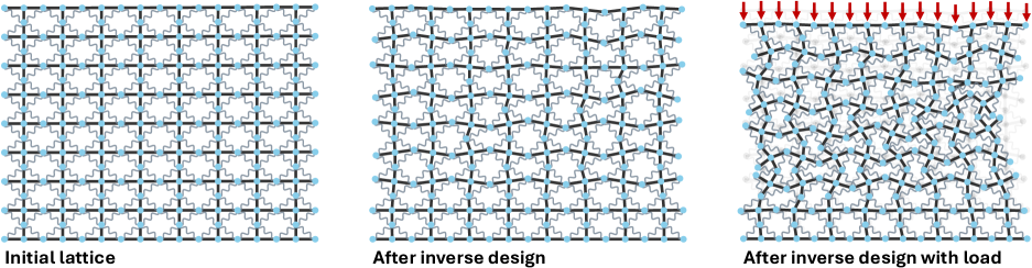
Figure S1: Reconfiguring a $8\times 8$ Totimorphic lattice from a Poisson’s ratio of $0$ to $-2$.

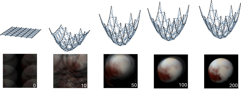
Figure S2: Initial reconfiguration from a flat surface to a curved mirror after 0, 10, 50, 100, and 200 update steps. Both the lattice configuration (top) and an image produced by the mirror at this configuration stage (bottom) are shown.

S5 Supplementary videos

S5.1 Video S1a caption

Using gradient descent, the Totimorphic lattice reconfigures to attain a Poisson’s ratio of $-0.5$.

S5.2 Video S1b caption

Using gradient descent, the Totimorphic lattice reconfigures to attain a Poisson’s ratio of $0.5$.

S5.3 Video S2a caption

Compression experiment with the Totimorphic configuration with Poisson’s ratio of $-0.5$.

S5.4 Video S2b caption

Compression experiment with the Totimorphic configuration with Poisson’s ratio of $0.5$.

S5.5 Video S3a caption

Initial deployment of the Totimorphic lattice from a collapsed to a flat configuration, which is then reconfigured to focus light at a distance of $20D$, where $D$ is the side length of the lattice. On the left, a zoom-in of the lattice is shown. The origin of the lattice is also a trainable parameter, which leads to minor movement of the lattice. This could be reduced by increasing the regularisation strength (or choosing the central point in the lattice as the origin and freezing it during optimisation). On the right, the reflected light is shown. The red dot indicates the target focal point.

S5.6 Video S3b caption

Reconfiguration of the Totimorphic lattice from a focal length of $2D$ to $1D$. On the left, a zoom-in of the lattice is shown. On the right, the reflected light is shown. The red dot indicates the target focal point.

References

- [1] Lorna J Gibson, Michael F Ashby and Brendan A Harley “Cellular materials in nature and medicine” Cambridge University Press, 2010
- [2] Ulrike GK Wegst et al. “Bioinspired structural materials” In Nature materials 14.1 Nature Publishing Group, 2015, pp. 23–36 DOI: 10.1038/nmat4089
- [3] James Utama Surjadi et al. “Mechanical metamaterials and their engineering applications” In Advanced Engineering Materials 21.3 Wiley Online Library, 2019, pp. 1800864
- [4] Lucas R Meza, Satyajit Das and Julia R Greer “Strong, lightweight, and recoverable three-dimensional ceramic nanolattices” In Science 345.6202 American Association for the Advancement of Science, 2014, pp. 1322–1326
- [5] Hamidreza Yazdani Sarvestani et al. “Bioinspired Stochastic Design: Tough and Stiff Ceramic Systems” In Advanced Functional Materials 32.6, 2022, pp. 2108492 DOI: 10.1002/adfm.202108492
- [6] Ashley M Torres et al. “Bone-inspired microarchitectures achieve enhanced fatigue life” In Proceedings of the National Academy of Sciences 116.49 National Acad Sciences, 2019, pp. 24457–24462
- [7] Elissa Ross and Daniel Hambleton “Using Graph Neural Networks to Approximate Mechanical Response on 3D Lattice Structures” In Proceedings of AAG2020-Advances in Architectural Geometry 24, 2021, pp. 466–485
- [8] Marco Maurizi, Chao Gao and Filippo Berto “Inverse design of truss lattice materials with superior buckling resistance” In npj Computational Materials 8.1 Nature Publishing Group UK London, 2022, pp. 247
- [9] Dominik Dold and Derek Aranguren van Egmond “Differentiable graph-structured models for inverse design of lattice materials” In Cell Reports Physical Science 4.10 Elsevier, 2023 DOI: https://doi.org/10.1016/j.xcrp.2023.101586
- [10] Sergei Shumilin, Alexander Ryabov, Evgeny Burnaev and Vladimir Vanovskii “A Method for Auto-Differentiation of the Voronoi Tessellation” In arXiv preprint arXiv:2312.16192, 2023
- [11] Li Zheng, Konstantinos Karapiperis, Siddhant Kumar and Dennis M Kochmann “Unifying the design space and optimizing linear and nonlinear truss metamaterials by generative modeling” In Nature Communications 14.1 Nature Publishing Group UK London, 2023, pp. 7563
- [12] Yayati Jadhav et al. “Generative Lattice Units with 3D Diffusion for Inverse Design: GLU3D” In Advanced Functional Materials Wiley Online Library, 2024, pp. 2404165
- [13] Tommaso Ghidini “Materials for space exploration and settlement” In Nature materials 17.10 Nature Publishing Group UK London, 2018, pp. 846–850
- [14] In-Won Park et al. “Soll-e: A module transport and placement robot for autonomous assembly of discrete lattice structures” In 2023 IEEE/RSJ International Conference on Intelligent Robots and Systems (IROS), 2023, pp. 10736–10741 IEEE
- [15] Christine E Gregg et al. “Ultralight, strong, and self-reprogrammable mechanical metamaterials” In Science robotics 9.86 American Association for the Advancement of Science, 2024, pp. eadi2746
- [16] A Thomas, J Grover, D Izzo and D Dold “Totimorphic structures for space application” In Materials Research Proceedings 37 Materials Research Forum LLC
- [17] S Macrae Montgomery et al. “Magneto-mechanical metamaterials with widely tunable mechanical properties and acoustic bandgaps” In Advanced Functional Materials 31.3 Wiley Online Library, 2021, pp. 2005319
- [18] Shuai Wu et al. “Magnetically actuated reconfigurable metamaterials as conformal electromagnetic filters” In Advanced Intelligent Systems 4.9 Wiley Online Library, 2022, pp. 2200106
- [19] Liwei Wang et al. “Physics-aware differentiable design of magnetically actuated kirigami for shape morphing” In Nature Communications 14.1 Nature Publishing Group UK London, 2023, pp. 8516
- [20] Shuyuan Xiao et al. “Active metamaterials and metadevices: a review” In Journal of Physics D: Applied Physics 53.50 IOP Publishing, 2020, pp. 503002
- [21] Xiaoxing Xia, Christopher M Spadaccini and Julia R Greer “Responsive materials architected in space and time” In Nature Reviews Materials 7.9 Nature Publishing Group UK London, 2022, pp. 683–701
- [22] Gaurav Chaudhary, S Ganga Prasath, Edward Soucy and L Mahadevan “Totimorphic assemblies from neutrally stable units” In Proceedings of the National Academy of Sciences 118.42 National Acad Sciences, 2021, pp. e2107003118 DOI: https://doi.org/10.1073/pnas.2107003118
- [23] Ryan H Lee, Erwin AB Mulder and Jonathan B Hopkins “Mechanical neural networks: Architected materials that learn behaviors” In Science Robotics 7.71 American Association for the Advancement of Science, 2022 DOI: 10.1126/scirobotics.abq7278
- [24] Ke Liu et al. “Triclinic metamaterials by tristable origami with reprogrammable frustration” In Advanced Materials 34.43 Wiley Online Library, 2022, pp. 2107998
- [25] Edward Mettler, William G Breckenridge and Marco B Quadrelli “Large aperture space telescopes in formation: modeling, metrology, and control” In The Journal of the Astronautical Sciences 53.4 Springer, 2005, pp. 391–412
- [26] Mark Ayre, Dario Izzo and Lorenzo Pettazzi “Self assembly in space using behaviour based intelligent components” In TAROS, Towards Autonomous Robotic Systems Citeseer, 2005
- [27] Camille Pirat et al. “Toward the autonomous assembly of large telescopes using cubesat rendezvous and docking” In Journal of Spacecraft and Rockets 59.2 American Institute of AeronauticsAstronautics, 2022, pp. 375–388
- [28] Ariel Ekblaw, Joe Paradiso, David Zuniga and Keith Crooker “Self-Assembling and Self-Regulating Space Stations: Mission Concepts for Modular, Autonomous Habitats”, 2021 50th International Conference on Environmental Systems
- [29] Brian P Trease et al. “Accommodating Thickness in Origami-Based Deployable Arrays”, 2013
- [30] Shannon A Zirbel, Brian P Trease, Spencer P Magleby and Larry L Howell “Deployment methods for an origami-inspired rigid-foldable array” In The 42nd Aerospace Mechanism Symposium, 2014
- [31] Andreas Öchsner and Resam Makvandi “Finite elements for truss and frame structures: an introduction based on the computer algebra system Maxima” Springer, 2018 DOI: 10.1007/978-3-319-94941-3
- [32] Sebastian Rabien “Adaptive parabolic membrane mirrors for large deployable space telescopes” In Applied Optics 62.11 Optica Publishing Group, 2023, pp. 2835–2844
- [33] Jane Rigby et al. “The science performance of JWST as characterized in commissioning” In Publications of the Astronomical Society of the Pacific 135.1046 IOP Publishing, 2023, pp. 048001
- [34] John Platt and Alan Barr “Constrained differential optimization” In Neural Information Processing Systems, 1987
- [35] Klaus Schittkowski “NLPQL: A FORTRAN subroutine solving constrained nonlinear programming problems” In Annals of operations research 5 Springer, 1986, pp. 485–500
- [36] David Baraff and Andrew Witkin “Large steps in cloth simulation” In Seminal Graphics Papers: Pushing the Boundaries, Volume 2, 2023, pp. 767–778
- [37] Dario Izzo and Lorenzo Pettazzi “Autonomous and distributed motion planning for satellite swarm” In Journal of Guidance, Control, and Dynamics 30.2, 2007, pp. 449–459