Comparing the 3D morphology of solid-oxide fuel cell anodes for different manufacturing processes, operating times, and operating temperatures

Abstract

Solid oxide fuel cells (SOFCs) are becoming increasingly important due to their high electrical efficiency, the flexible choice of fuels and relatively low emissions of pollutants. However, the increasingly growing demands for electrochemical devices require further performance improvements. Since it is well known that the 3D morphology of the electrodes, which is significantly influenced by the underlying manufacturing process, has a profound impact on the resulting performance, a deeper understanding for the structural changes caused by modifications of the manufacturing process or degradation phenomena is desirable. In the present paper, we investigate the influence of the operating time and the operating temperature on the 3D morphology of SOFC anodes using 3D image data obtained by focused-ion beam scanning electron microscopy, which is segmented into gadolinium-doped ceria, nickel and pore space. In addition, structural differences caused by manufacturing the anode via infiltration or powder technology, respectively, are analyzed quantitatively by means of various geometrical descriptors such as specific surface area, length of triple phase boundary per unit volume, mean geodesic tortuosity, and constrictivity. The computation of these descriptors from 3D image data is carried out both globally as well as locally to quantify the heterogeneity of the anode structure.

¹ Institute of Stochastics, Ulm University, 89069 Ulm, Germany
² Institute of Energy Materials and Devices, IMD-2: Materials Synthesis and Processing, 52428 Jülich, Germany
³ Institute for Applied Materials (IAM-ET), Karlsruhe Institute of Technology (KIT), 76131 Karlsruhe, Germany
⁴ Robert Bosch GmbH (BOSCH), Zentrum für Forschung und Vorausentwicklung, 71272 Renningen, Germany
⁵ Institute for Applied Materials (IAM-MMS), Karlsruhe Institute of Technology (KIT), 76131 Karlsruhe, Germany

Keywords— solid oxide fuel cell; 3D morphology; FIB-SEM; anode; degradation; aging; statistical image analysis

1 Introduction

Solid oxide fuel cells (SOFCs) are becoming increasingly important due to their high electrical efficiency, the flexible choice of fuels and relatively low emissions of pollutants [1, 2, 3, 4]. Thus, applications of SOFCs range from stationary power generation in the private as well as the industrial sector to electric vehicles, where they can be considered as emerging technology. However, the steadily growing demands for electrochemical devices in combination with open problems such as pronounced degradation mechanisms require further technological progress to unlock the full potential of fuel cells as an efficient alternative to traditional fossil fuel-based energy sources[5, 6]. One possibility to achieve this goal is the transition towards novel materials as for example the replacement of yttria-stabilized zirconia (YSZ) by gadolinium-doped ceria (GDC), which offers a higher ionic conductivity at lower temperatures compered to YSZ [7, 8, 9, 10]. This also reduces thermal degradation effects and thus increases the durability of SOFCs. Besides further optimizing the performance of SOFCs via improving the properties of the underlying materials, tuning the 3D morphology of the electrodes is a promising strategy since it is well known that the 3D morphology has a profound impact on fuel transport within the pore space, electric transport as well as ionic transport within the electrolyte [11, 12, 13, 14]. Moreover, not only the spatial distribution of each phase is of interest, but also the length of the triple-phase boundary (TPB), where the chemical reaction mainly takes place. More precisely, at the anode the fuel gas (typical choices are hydrogen or methane) is oxidized, which results in electrons that are transported to the cathode through an external circuit. At the cathode, these electrons are used to power the reduction reaction of oxygen, which react to oxygen ions. In order to quantitatively characterize the 3D morphology of SOFC electrodes at the relevant scale, focused ion beam scanning electron microscopy (FIB-SEM) is a frequent choice [15, 16, 17, 18, 19]. In particular, it turned out that local heterogeneities of electrodes have a profound impact on the resulting performance [20, 21, 22].

In the present paper, we consider eight GDC-based SOFC anodes, which are imaged via 3D FIB-SEM. The resulting image data is used as a basis for a comprehensive structural characterization of these anodes, which differ with regard to their operating conditions (i.e., operating temperature and operating time) and the underlying manufacturing process (powder technology or infiltration). The quantitative structural analysis of these SOFC anodes by means of various geometrical descriptors allows for a deeper understanding of process-structure relationships and degradation phenomena, which is crucial for the design of SOFC anodes with improved electrochemical properties.

The rest of this paper is organized as follows. In Section 2, the manufacturing process of the SOFC anodes including the underlying materials and the operating conditions, the imaging via 3D FIB-SEM and the segmentation of the resulting image data into nickel, GDC and pore space is explained. Next, the geometrical descriptors that are used for the quantitative structural analysis of the anodes - including, among others, volume fraction, specific surface area, and mean length of TPB per unit volume - are presented in Section 3. Section 4 contains a detailed, quantitative analysis of the influence of the operating temperature, the operating time, as well as the manufacturing process on the resulting 3D morphology of the anodes. Finally, the paper is concluded by a summary of the main results and an outlook to future research activities.

2 Experimental

This section covers the description of the manufacturing processes for seven SOFC anodes, including underlying materials as well as operating conditions (Section 2.1), tomographic imaging via 3D FIB-SEM (Section 2.2) and, finally, segmentation of the 3D image data into nickel, GDC and pore space (Section 2.3).

2.1 Electrode materials, manufacturing and aging

In the present paper, two different manufacturing processes for SOFC anodes are considered: powder technology and infiltration.

In the first case, symmetrical cells consisting of an 8 mol-% YSZ electrolyte from the company Kerafol^© (Eschenbach i.d.Opf., Germany) sandwiched in between GDC interlayers were produced. The GDC powder ($\mathsf{Gd}_{0.1}\mathsf{Ce}_{0.9}\mathsf{O}_{1.95}$) was commercially available from Fuelcellmaterials and transformed into a paste by the standard procedure of Forschungszentrum Jülich GmbH, using $\alpha$-terpineole as a dispersion medium and ethylcellulose as a transport medium. The functional layer (50 w% NiO, 50 w% GDC ) was produced in the same way using, commercially available GDC powder ($\mathsf{Gd}_{0.1}\mathsf{Ce}_{0.9}\mathsf{O}_{1.95}$) from Fuelcellmaterials and $\mathsf{NiO}$ powder from G. Vogler B.V. in a 50:50 w% ratio.

For the infiltration experiment, an additional $\mathsf{NiO}$ layer was screen printed on both sides of the GDC sandwiched 8 mol-% YSZ electrolyte. The infiltration of the $\mathsf{NiO}$ layer was conducted, using a $\mathsf{GDC}(\mathsf{NO}_{3})_{3}$ solution ($3\text{\,}\mathrm{mol}$). Therefore, the cells were immersed into the solution for about five minutes under vacuum, dried and sintered at $500\text{\,}\mathrm{\SIUnitSymbolCelsius}$ for $3\text{\,}\mathrm{h}$. Different sintering temperatures for the scaffold were used and a variety of repetitions for the infiltration steps was tested. In the above-described cases, an additional contact layer of $\mathsf{NiO}$ was added on top, using screen printing method and dried at $80\text{\,}\mathrm{\SIUnitSymbolCelsius}$ overnight.

In case of the SOFC anodes manufactured via the infiltration process, the cells were gradually heated in a mixture of $95\text{\,}\mathrm{\char 37\relax}$ $\mathsf{N}_{2}$ and $5\text{\,}\mathrm{\char 37\relax}$ $\mathsf{H}_{2}$ at a rate of $1\text{\,}\mathrm{K}\text{\,}{\mathrm{min}}^{-1}$ until reaching $650\text{\,}\mathrm{\SIUnitSymbolCelsius}$. At this temperature, the gas composition was changed to $65\text{\,}\mathrm{\char 37\relax}$ $\mathsf{N}_{2}$, $$30\text{\,}\mathrm{\char 37\relax}$\mathsf{H}_{2}$, and $$5\text{\,}\mathrm{\char 37\relax}$\mathsf{H}_{2}\mathsf{O}$ and maintained for six hours. Subsequently, the gas composition was adjusted to $3.7\text{\ }{10}^{-4}\text{\,}\mathrm{mol}\text{\,}{\mathrm{s}}^{-1}$ of hydrogen and $9.2\text{\ }{10}^{-5}\text{\,}\mathrm{mol}\text{\,}{\mathrm{s}}^{-1}$ of oxygen to create a 1:1 hydrogen/steam mixture. Electrochemical impedance spectroscopy (EIS) was then used to characterize the cells at $650\text{\,}\mathrm{\SIUnitSymbolCelsius}$ and $600\text{\,}\mathrm{\SIUnitSymbolCelsius}$, see [23] for further details. Two of the three cells, which are manufactured via the infiltration process, were subjected to additional high-temperature treatments under the aging conditions detailed in Table 2 of [24]. During the aging process, reference impedance measurements at $600\text{\,}\mathrm{\SIUnitSymbolCelsius}$ were conducted on both cells every few hundred hours.

2.2 Tomographic imaging

Tomographic imaging has been carried out with 3D FIB-SEM using a Helios 5 Hydra DualBeam (ThermoFisher) with a concentric backscatter detector. An acceleration voltage of $3\text{\,}\mathrm{keV}$ and a current of $0.8\text{\,}\mathrm{nA}$ is used. Some samples have been imaged with a voxel size of $20\text{\,}\mathrm{nm}$ and some with $50\text{\,}\mathrm{nm}$, see Table 1 for a detailed overview of all considered anode samples.

manufacturing process	reduction temp. [$\text{\,}\mathrm{\SIUnitSymbolCelsius}$]	operating time [$\text{\,}\mathrm{h}$]	operating temp. [$\text{\,}\mathrm{\SIUnitSymbolCelsius}$]	voxel size [$\text{\,}\mathrm{nm}$]
powder	800	0	-	50
powder	800	240	900	50
powder	800	1100	900	50
infiltration	650	640	900	20
infiltration	650	0	-	20
infiltration	650	1000	700	20
powder	650	0	-	20

Table 1: Sample information including manufacturing process, reduction temperature, operating time, operating temperature and voxel size.

2.3 Image processing

At first, the 3D grayscale image data has been denoised using a total variation filter with a denoising weight of 50 [25]. Next, the grayvalue histogram of the denoised 3D image is computed and partitioned into five regions, namely pore markers, nickel markers, GDC markers and two intermediate regions. Each of the two intermediate regions corresponds to 10% of all voxels with grayvalues, where one can not yet distinguish between pore space and nickel or between nickel and GDC , respectively. Next, markers are removed if they are close to some interface, which is quantified by the upper 20 % quantile of highest gradient values. Note that the edge magnitude using the Scharr transform is exploited to compute the gradient [26]. Moreover, markers are removed near “cracks”, which is defined as highest 2 % (in case of the samples with a voxel size of $20\text{\,}\mathrm{nm}$) or 5 % (in case of the samples with a voxel size of $50\text{\,}\mathrm{nm}$) values after Meijering filtering [27]. The remaining markers are then used as markers for the watershed algorithm, where the input image is given by the gradient image [28].

3 Geometrical descriptors

In order to quantify the 3D morphology of the SOFC anodes considered in this paper, various geometrical descriptors are used. For this, the three phases, i.e., nickel, GDC and pores, are considered as realizations of random closed sets (RACSs) in the three-dimensional Euclidean space $\mathbb{R}^{3}$. These RACSs are assumed to be motion-invariant, i.e., stationary and isotropic, and denoted by $\Xi_{1},\Xi_{2}$ and $\Xi_{3}$, respectively. Moreover, in the definition of some geometrical descriptors, we even assume that the vector $(\Xi_{i},\Xi_{j})$ is motion-invariant for any $i,j\in\{1,2,3\}$. On the other hand, in some cases, the assumption of stationarity is sufficient. A formal introduction to the theory of stationary and isotropic RACSs can be found in [29].

Volume fraction

One of the most fundamental geometrical descriptors of stationary RACSs is their volume fraction. Furthermore, the volume fractions of the three anode phases mentioned above have a profound impact on the performance of SOFCs. In the following, the volume fraction of a stationary RACS will be denoted by $\varepsilon$. It can be easily estimated from voxelized 3D image data via the point-count method [30].

Specific surface area

Similar to volume fractions, the specific surface areas (SSAs) of the three anode phases are also of importance with regard to the performance of SOFCs, where this geometrical descriptor is defined as the mean surface area of a predefined phase per unit volume. It will be denoted by $S$ in the following. For the estimation of $S$ from voxelized 3D image data, locally weighted $2\times 2\times 2$ voxel configurations are used, see [31] for details regarding the choice of the weights. Besides the SSA of a certain phase, the specific interfacial area between two phases is also of interest. Note that in case of the three-phase anode material, which is modeled by the stationary RACSs $\Xi_{1},\Xi_{2}$ and $\Xi_{3}$, the specific interfacial area $S(\Xi_{i}\cap\Xi_{j})$ between phases $i$ and $j$ with $i,j\in\{1,2,3\}$ and $i\neq j$ can be determined via the following equation:

$$S(\Xi_{i}\cap\Xi_{j})=\frac{1}{2}\Bigl{(}S(\Xi_{i})+S(\Xi_{j})-S(\Xi_{k})\Bigr{)},$$ (1)

where $k=\{1,2,3\}\backslash\{i,j\}$.

Triple-phase boundary length

Since the chemical reaction in SOFC anodes takes place at the triple-phase boundary (TPB), the expected length of TPB per unit volume is of particular interest. It is called specific length of TPB in the following and defined as

$$\ell_{\mathsf{TPB}}=\mathbb{E}\left(\mathcal{H}_{1}(\Xi_{1}\cap\Xi_{2}\cap\Xi_{3}\cap[0,1]^{3})\right),$$

where $\mathcal{H}_{1}$ denotes the one-dimensional Hausdorff measure in $\mathbb{R}^{3}$. This geometrical descriptor is estimated from 3D image data by first detecting all $2\times 2\times 2$ voxel configurations, which contain at least one voxel of each of the three phases. Next, each pair of these voxel configurations that are neighbors with respect to the 6-neighborhood is determined. Finally, the number of these pairs is divided by the total number of voxels in the sampling window.

Geodesic tortuosity

In SOFC anodes, three kinds of transport processes take place: The transport of the transport of the gaseous educts and products within the pore space, the transport of oxygen ions within the GDC phase, and the transport of electrons, which mainly takes place within the nickel phase. A geometrical descriptor that turned out useful to characterize various types of transport phenomena in porous media is connected with the tortuosity, i.e., the windedness of their phases. Note that there exist several notions of tortuosity in the literature [32]. In the present paper, we consider the so-called geodesic tortuosity, which is a purely geometric descriptor of 3D morphologies. More precisely, a starting plane and a target plane, which is parallel to the starting plane, are chosen. Next, for a given phase of the material, the shortest path to the target plane is determined for each point of this phase within the starting plane. Then, the lengths of these shortest paths are normalized by dividing them by the distance between both planes. This results in the distribution of geodesic tortuosity, the mean value of which will be denoted by $\tau$. A formal definition of geodesic tortuosity within the framework of random closed sets is presented in [33]. Note that the computation of this geometrical descriptor from voxelized 3D image data is carried out by means of Dijkstra’s algorithm [34].

Moreover, two modifications of geodesic tortuosity are considered. On the one hand, we consider the so-called dilated geodesic tortuosity, where we just investigate the lengths of those paths along which there is a certain minimum distance $r>0$ to the complement of the given transport phase. On the other hand, only paths to the target plane are considered which start from the TPB, since the majority of transport processes are either targeting the TPB or starting at the TPB.

Constrictivity

The constrictivity of a transport phase, denoted by $\beta\in[0,1]$, is a measure for the strength of bottleneck effects. It is defined as $\beta=\left(r_{\mathsf{min}}/r_{\mathsf{max}}\right)^{2}$, where $\beta=1$ corresponds to the case that no bottleneck effects exist, and a value of $\beta$ close to zero indicates pronounced bottleneck effects [35]. The quantity $r_{\mathsf{max}}$ appearing in this formula is related with the continuous pore size distribution function $\mathsf{CPSD}:[0,\infty)\to[0,1]$ of a stationary RACS $\Xi\subset\mathbb{R}^{3}$ [36, 37]. Here, for each $r\geq 0$, the subset $\Xi\circ B(o,r)$ of $\Xi$ is considered, which can be covered by (potentially overlapping) spheres with radius $r$, where $B(o,r)\subset\mathbb{R}^{3}$ is the sphere with midpoint at the origin $o\in\mathbb{R}^{3}$ and radius $r\geq 0$, and $\circ$ denotes morphological opening. The value $\mathsf{CPSD}(r)$ is then defined as the volume fraction of the stationary RACS $\Xi\circ B(o,r)$, and $r_{\mathsf{max}}=\sup\{r\geq 0:\mathsf{CPSD}(r)\geq 0.5\ \mathsf{CPSD}(0)\}$. On the other hand, the definition of the characteristic bottleneck radius $r_{\mathsf{min}}$ is based on the simulated mercury intrusion porosimetry $\mathsf{SMIP}:[0,\infty)\to[0,1]$, which is closely related to CPSD, but additionally depends on a predefined direction. More precisely, the value $\mathsf{SMIP}(r)$ is defined as the volume fraction of the subset of the $\Xi$, which can be reached by an intrusion of spheres with radius $r$ from the predefined direction. Analogously to $r_{\mathsf{max}}$, the radius $r_{\mathsf{min}}$ is defined as $r_{\mathsf{min}}=\sup\{r\geq 0:\mathsf{SMIP}(r)\geq 0.5\ \mathsf{CPSD}(0)\}$.

Two-point coverage probability function

Another frequently used geometrical descriptor is the two-point coverage probability function. More precisely, let $\Xi_{i}$ and $\Xi_{j}$ be two RACSs such that the vector $(\Xi_{i},\Xi_{j})$ is motion-invariant, for all $i,j\in\{1,2,3\}$. The two-point coverage probability function $\tilde{C}_{i,j}:[0,\infty)\to[0,1]$ is then defined by $\tilde{C}_{i,j}(r)=\mathbb{P}(o\in\Xi_{i},h\in\Xi_{j})$, where $h\in\mathbb{R}^{3}$ is an arbitrary vector of length $r\geq 0$. In particular, the value of $\tilde{C}_{i,j}(r)$ only depends on the distance $r\geq 0$ between two points due to the assumed motion-invariance of $(\Xi_{i},\Xi_{j})$. Note that the limit of $\tilde{C}_{i,j}(r)$ for $r\to\infty$ is often equal to the product $\varepsilon_{i}\varepsilon_{j}$ of the volume fractions $\varepsilon_{i}$ and $\varepsilon_{j}$ of $\Xi_{i}$ and $\Xi_{j}$, respectively, since in case of the vast majority of materials the events that $o\in\Xi_{j}$ and $h\in\Xi_{j}$ are becoming stochastically independent for unboundedly increasing distances $r$. Thus, in the following, we consider the centered two-point coverage probability function $C_{i,j}:[0,\infty)\to[0,1]$, which is defined as $C_{i,j}(r)=\tilde{C}_{i,j}(r)-\varepsilon_{i}\varepsilon_{j}$ for each $r\geq 0$. i.e., there is a positive correlation between the events $o\in\Xi_{i}$ and $h\in\Xi_{j}$ if $C_{i,j}(r)>0$, and vice versa. The estimation of the values of $C_{i,j}$ from voxelized image data is carried out via a Fourier-based method described in [38].

Chord length distribution

The chord length distribution of a motion-invariant RACS $\Xi$ is defined as the distribution of the length of segments chosen at random in $\Xi\cap\ell$, where $\ell$ is some line passing through the origin Due to the isotropy of $\Xi$, the chord length distribution does not depend on the specific choice of the direction of the intersecting line $\ell$. Thus, in the following, only chords in the direction of the $x$-axis are considered. To estimate the chord length distribution from voxelized image data, we use the algorithms proposed in [39, 38].

Spherical contact distance

The cumulative distribution function $H:[0,\infty)\to[0,1]$ of spherical contact distances of a stationary RACS $\Xi$ is defined as

$$H(r)=1-\mathbb{P}(o\notin\Xi\oplus B(o,r)\mid o\notin\Xi)\qquad\text{ for each }r\geq 0,$$

where $\oplus$ denotes Minkowski addition, i.e., the value of $H(r)$ is the probability that the distance from a randomly chosen point of the complement of $\Xi$ to the nearest point of $\Xi$ is not longer than $r$. Thus, this geometrical descriptor can be used in order to quantify the compactness/perforation of a geometrically complex phase. When estimating the spherical contact distribution from voxelized 3D image data, the Euclidean distance transform is computed and the algorithm described in [40] is applied.

Local geometrical descriptors

Besides computing the geometrical descriptors mentioned above, just once for each of the entire 3D images corresponding to the eight SOFC anode samples considered in this paper, we additionally compute some of these descriptors locally to quantify the heterogeneity of the SOFC anodes. More precisely, the 3D image data is partitioned into non-overlapping cutouts. For this purpose, we consider cubic cutouts with a size of $64$ voxel in each direction. Thus, for a voxel size of $20\text{\,}\mathrm{nm}$ and $50\text{\,}\mathrm{nm}$, we get cubic cutouts with a side length of $1.28\text{\,}\mathrm{\SIUnitSymbolMicro m}$ and $3.2\text{\,}\mathrm{\SIUnitSymbolMicro m}$, respectively.

4 Results and discussion

We now use the geometrical descriptors stated in Section 3 in order to investigate the influence of operating temperature, operating time and the manufacturing process on the 3D morphology of SOFC anodes. Therefore, subsets of samples from the eight SOFC anode samples considered in this paper, which differ in exactly one of these influencing factors, are quantitatively compared to each other with respect to the geometrical descriptors of Section 3. Note that in the figures presented below, results regarding the nickel phase are always shown in blue, whereas those regarding the GDC phase are shown in red, and those regarding the pore space in yellow.

4.1 Influence of operating temperature

To begin with, we investigate the influence of operating temperature on the 3D morphology of SOFC anodes, where we consider only samples manufactured by means of the infiltration process, a reduction temperature of $650\text{\,}\mathrm{\SIUnitSymbolCelsius}$ and a voxel size of $20\text{\,}\mathrm{nm}$. Under these conditions, we compare the samples with an operating temperature of $700\text{\,}\mathrm{\SIUnitSymbolCelsius}$ and $900\text{\,}\mathrm{\SIUnitSymbolCelsius}$, respectively, where the 3D morphology of these samples is visualized in Figure 1. However, note that the operating time also differs for these two samples. For the sample with operating temperature of $700\text{\,}\mathrm{\SIUnitSymbolCelsius}$ the operating time is $1000\text{\,}\mathrm{h}$, while the operating time of the sample with operating temperature of $900\text{\,}\mathrm{\SIUnitSymbolCelsius}$ is only $640\text{\,}\mathrm{h}$. Nonetheless, the comparison of these two samples is reasonable, since polarization resistance measured at $900\text{\,}\mathrm{\SIUnitSymbolCelsius}$ increased only slightly during the last $310\text{\,}\mathrm{h}$, which indicates just negligible structural changes.

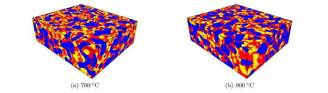
Figure 1: 3D morphology of SOFC anodes, consisting of nickel (blue), GDC (red) and pore space (yellow), for operating temperatures of $700\text{\,}\mathrm{\SIUnitSymbolCelsius}$ (a) and $900\text{\,}\mathrm{\SIUnitSymbolCelsius}$ (b). Both samples are manufactured by means of the infiltration process, reduced at a temperature of $650\text{\,}\mathrm{\SIUnitSymbolCelsius}$, and imaged with a voxel size of $20\text{\,}\mathrm{nm}$.

The upper row of Figure 2 shows that there are only small differences in volume fraction and constrictivity for the different operating temperatures. However, the specific length of TPB becomes significantly shorter for the higher operating temperature of $900\text{\,}\mathrm{\SIUnitSymbolCelsius}$. Furthermore, as a result of the higher operating temperature, the SSAs of the pore space and the associated interfaces are also significantly reduced. Thus, we observe a coarsening of the pore space. In combination with a significant decrease of the specific length of TPB, this indicates a worse electrochemical performance of the $900\text{\,}\mathrm{\SIUnitSymbolCelsius}$ sample, compared to the operating temperature of $700\text{\,}\mathrm{\SIUnitSymbolCelsius}$. On the other hand, the SSA of the interface between the nickel and GDC phases increases.

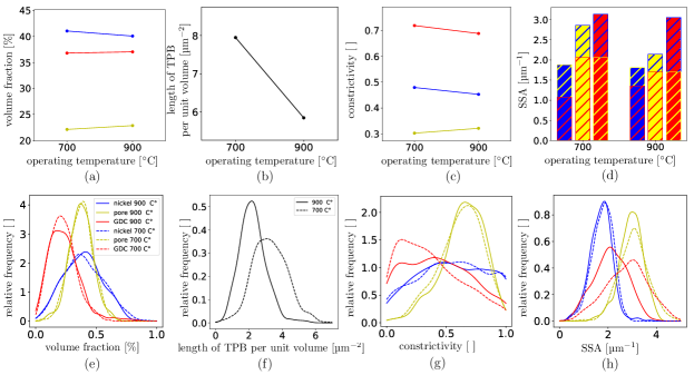
Figure 2: Geometrical descriptors of the three phases nickel (blue), GDC (red) and pore space (yellow) for different operating temperatures. Upper row: volume fraction (a), specific length of TPB (b), constrictivity (c), as well as SSA (d), which is divided into the contributions from the different interfaces through the hatching, is shown. Lower row: probability densities of local descriptors based on non-overlapping cubic cutouts of size $1.28\text{\,}\mathrm{\SIUnitSymbolMicro m}$.

The (global) geometrical descriptors considered in the upper row of Figure 2 have also been computed for non-overlapping cutouts with a size of $1.8\text{\,}\mathrm{\SIUnitSymbolMicro m}$. The resulting probability densities of local descriptors are shown in the lower row of Figure 2. Differences between these densities for the two operating temperatures are especially recognizable in volume fraction, SSA and constrictivity of the GDC phase, while the nickel phase and pore space show only small local differences. Furthermore, there are local differences in the specific length of TPB between the two operating temperatures, whereby the distribution of the local specific length of TPB is broader and its mean is shifted to the right-hand side for the operating temperature of $700\text{\,}\mathrm{\SIUnitSymbolCelsius}$, compared to $900\text{\,}\mathrm{\SIUnitSymbolCelsius}$.

In Figure 3, the mean geodesic tortuosity, the mean geodesic tortuosity of paths starting from TPB, and the dilated mean geodesic tortuosity with $r=$0.1\text{\,}\mathrm{\SIUnitSymbolMicro m}$$ are shown for all three phases in the respective transport direction. The mean geodesic tortuosities for the nickel and GDC phases change only slightly when changing the operating temperature, while the mean geodesic tortuosity of paths starting from the TPB increases for the pore space. This means that the transport properties have worsened, when the operating temperature is increased to $900\text{\,}\mathrm{\SIUnitSymbolCelsius}$. Note that the dilated mean geodesic tortuosity of pore space could not be computed, because the paths within the pore space are too narrow.

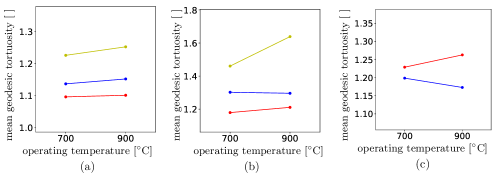
Figure 3: Mean geodesic tortuosity (a), mean geodesic tortuosity of paths starting from TPB (b), and dilated mean geodesic tortuosity with $r$ = $0.1\text{\,}\mathrm{\SIUnitSymbolMicro m}$ (c), for the three phases nickel (blue), GDC (red) and pores (yellow), for different operating temperatures.

In Figure 4, the cumulative distribution functions of spherical contact distance and chord length are shown for the three phases nickel, GDC and pores, as well as the centered two-point coverage probability functions for each of these phases, and for combinations of different phases, for an operating temperature of $700\text{\,}\mathrm{\SIUnitSymbolCelsius}$ and $900\text{\,}\mathrm{\SIUnitSymbolCelsius}$, respectively.

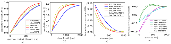
Figure 4: Cumulative distribution functions of spherical contact distance (a) and chord length (b) for the three phases nickel (blue), GDC (red) and pores (yellow), as well as centered two-point coverage probability functions for each of these phases (c), and for combinations of different phases (d), for an operating temperature of $700\text{\,}\mathrm{\SIUnitSymbolCelsius}$ and $900\text{\,}\mathrm{\SIUnitSymbolCelsius}$, respectively.

Again, like in Figure 3, for the nickel and GDC phases only slight changes of the descriptors considered in Figures 4a and 4b can be observed when increasing the operating temperature from $700\text{\,}\mathrm{\SIUnitSymbolCelsius}$ and $900\text{\,}\mathrm{\SIUnitSymbolCelsius}$, while the differences for the pore space are more pronounced, for both spherical contact distances and chord lengths. More precisely, for the pore space, an operating temperature of $900\text{\,}\mathrm{\SIUnitSymbolCelsius}$ leads to larger contact distances and longer chord lengths than an operating temperature of $700\text{\,}\mathrm{\SIUnitSymbolCelsius}$, which can be interpreted as coarsening of pore space. Furthermore, while the differences between the centered two-point coverage probability functions for the nickel and GDC phases are negligible when comparing these functions for the operating temperatures of $700\text{\,}\mathrm{\SIUnitSymbolCelsius}$ and $900\text{\,}\mathrm{\SIUnitSymbolCelsius}$, the centered two-point coverage probability function of the pore space decreases more slowly towards zero for $900\text{\,}\mathrm{\SIUnitSymbolCelsius}$ compared to its behavior for $700\text{\,}\mathrm{\SIUnitSymbolCelsius}$, see Figure 4 c. With regard to centered two-point coverage probability functions for combinations of different phases, it is noticeable that one observes a slower decrease towards zero for $900\text{\,}\mathrm{\SIUnitSymbolCelsius}$ than for $700\text{\,}\mathrm{\SIUnitSymbolCelsius}$ in case of both phase combinations including the pore space, see Figure 4d.

4.2 Influence of operating time

To investigate the influence of operating time on the 3D morphology of SOFC anodes, we consider the samples manufactured by means of powder technology and a reduction temperature of $800\text{\,}\mathrm{\SIUnitSymbolCelsius}$, which are aged with an operating temperature of $900\text{\,}\mathrm{\SIUnitSymbolCelsius}$ and imaged with a voxel size of $50\text{\,}\mathrm{nm}$. More precisely, we compare the 3D morphology of SOFC anodes in pristine state and after operating times of $240\text{\,}\mathrm{h}$ and $1100\text{\,}\mathrm{h}$, respectively. The 3D morphology of these three samples is visualized in Figure 5.

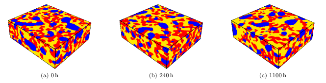
Figure 5: 3D morphology of SOFC anodes, consisting of nickel (blue), GDC (red) and pore space (yellow), which haven been manufactured by means of powder technology and aged with an operating temperature of $900\text{\,}\mathrm{\SIUnitSymbolCelsius}$ and operating times of $0\text{\,}\mathrm{h}$ (a), $240\text{\,}\mathrm{h}$ (b) and $1100\text{\,}\mathrm{h}$ (c), where imaging was done with a voxel size of $50\text{\,}\mathrm{nm}$.

The influence of operating time is investigated by means of various global geometrical descriptors, which have been computed on image data of the whole samples, as well as by means of local descriptors, see Figure 6.

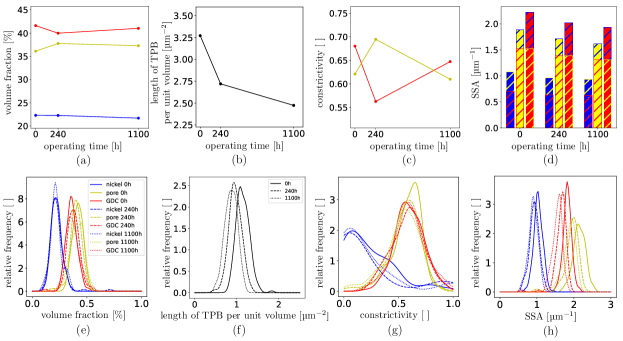
Figure 6: Geometrical descriptors of the three phases nickel (blue), GDC (red) and pore space (yellow) for different operating times. Upper row: volume fraction (a), specific length of TPB (b), constrictivity (c), as well as SSA (d), which is split into the contributions from the different interfaces through the hatching. Lower row: probability densities of local descriptors based on non-overlapping cubic cutouts of size $3.2\text{\,}\mathrm{\SIUnitSymbolMicro m}$.

It turned out that there are only negligible changes in the volume fraction for all three phases, see Figure 6a. But, on the other hand, it is noticeable that the specific length of TPB significantly decreases with increasing operating time, whereas the impact of operating time on constrictivity of GDC and pore space is less clear, see Figures 6b and 6c. However, for each operation time considered in this paper, the nickel phase is poorly connected, leading to a constricitivity of zero. Furhtermore, the SSAs of nickel and GDC as well as of the pore space are decreasing with increasing operating time, while the volume fractions remain almost unchanged, see Figures 6a and 6d, which means that the entire 3D morphology of the SOFC anodes is coarsening. This coarsening in combination with a significant decrease of the specific length of TPB indicates a worse electrochemical performance for longer operating times. In the lower row of Figure 6, the probability densities of local geometrical descriptors are shown, which have been computed for non-overlapping cubic cutouts of size $3.2\text{\,}\mathrm{\SIUnitSymbolMicro m}$, where slight differences can be observed for all descriptors of the three phases and for all operating times. For example, the probability density of the local specific length of TPB is shifted to the left for longer operating times, see Figures 6f. This means that the local specific lengths of TPB tend to become shorter locally with increasing operating time. We also remark that the nickel phase is locally better connected than globally, which is indicated by the fact that there is a subset of the unit interval $[0,1]$ where the values of the probability density of local constrictivity of the nickel phase are greater than zero, see Figure 6g.

To examine the transport capability within the three phases, the three different types of geodesic tortuosity explained in Section 3 are considered. While the nickel phase is too disconnected to determine a mean geodesic tortuosity for the operating time of $240\text{\,}\mathrm{h}$, the corresponding mean geodesic tortuosity of paths starting from the TPB can be computed, but has a high value, see Figures 7a and 7b. Moreover, the dilated mean geodesic tortuosity with $r=$0.1\text{\,}\mathrm{\SIUnitSymbolMicro m}$$ cannot be computed for the nickel phase in case of all operating times, see Figure 7c, which indicates that the existing paths in the nickel phase are rather narrow. Thus, the poor connection and the narrow paths in the nickel phase indicate that the electric transport properties of this phase are rather poor. In contrast, the GDC phase and the pore space have a relatively low mean geodesic tortuosity values with regard to all three types of geodesic tortuosity.

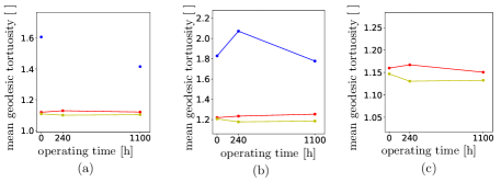
Figure 7: Mean geodesic tortuosity (a), mean geodesic tortuosity of paths starting from TPB (b), dilated mean geodesic tortuosity with $r=$0.1\text{\,}\mathrm{\SIUnitSymbolMicro m}$$ (c), for nickel (blue), GDC (red), and pores (yellow).

Furthermore, the distributions of spherical contact distances and chord lengths have been analyzed to investigate the impact of operating time on the 3D morphology of SOFC anodes. For all three phases, the spherical contact distances tend to increase with increasing operating time, see Figure 8a. Similarly, in comparison to the pristine state, the chord lengths get longer during operation, especially for the nickel phase, see Figure 8b. Thus, also these observations indicate a coarsening of the phases in the course of fuel cell operation.

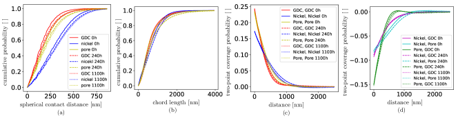
Figure 8: Cumulative distribution functions of spherical contact distance (a) and chord length (b) for nickel (blue), GDC (red) and pores (yellow), as well as centered two-point coverage probability functions for each of these phases (c) and for combinations of different phases (d).

Examining the centered two-point coverage probability functions of the individual phases shows that the values of these functions increase with increasing operating time, see Figure 8c. Interestingly, this increase is more pronounced during shorter operating times indicating more pronounced structural changes at the early stage of operation compared to the later one. Examining the centered two-point coverage probability functions of two different phases, it turns out that they are shrinking with increasing operating time, see Figure 8d. Thus, again a coarsening of the 3D anode morphology with increasing operating time is indicated.

4.3 Influence of manufacturing process

Last but not least, we compare the 3D morphologies of pristine SOFC anodes prepared by means of two different manufacturing processes, i.e., powder technology and infiltration, where 3D image data of pristine samples with a voxel size of $20\text{\,}\mathrm{nm}$ are used, see Figure 9.

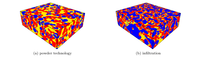
Figure 9: 3D morphology of pristine SOFC anodes prepared by powder technology (a) and infiltration (b), comprising nickel (blue), GDC (red), and pores (yellow).

First, to investigate the influence of the manufacturing process on the 3D morphology of the anodes, geometrical descriptors are computed on the whole anode samples. It is striking that the volume fractions of the three phases (nickel, GDC and pores) differ significantly for the two samples prepared by the different manufacturing processes. For example, the volume fraction of nickel phase in the SOFC anode manufactured by infiltration is roughly $40\text{\,}\mathrm{\char 37\relax}$, while it is halved for the SOFC anode manufactured by means of the powder technology, see Figure 10a.

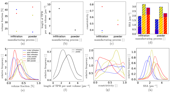
Figure 10: Geometrical descriptors of the three phases nickel (blue), GDC (red) and pore space (yellow) for different manufacturing processes. Upper row: volume fraction (a), specific length of TPB (b), constrictivity (c) as well as SSA (d), which is split into the contributions from the different interfaces through the hatching. Lower row: probability densities of local descriptors based on non-overlapping cutouts of size $1.28\text{\,}\mathrm{\SIUnitSymbolMicro m}$.

Moreover, as shown in Figure 10b, infiltration leads to a significantly larger specific length of TPB than powder technology. Besides this, the nickel phase obtained by powder technology is very disconnected such that its constrictivity is equal to zero, while infiltration leads to a (small) positive constrictivity value of the nickel phase, see Figure 10c. Furthermore, note that the different manufacturing processes also cause differences in the SSA, see Figure 10d. In particular, the fraction of nickel-GDC interface and the SSAs of all three phases are smaller when using powder technology instead of infiltration. Thus, altogether, infiltration leads to a more desirable 3D morphology of SOFC anodes with regard to chemical reaction surfaces. For non-overlapping cutouts of size $1.28\text{\,}\mathrm{\SIUnitSymbolMicro m}$, the corresponding probability densities of local geometrical descriptors are shown in the lower row of Figure 10. Also here, it is clearly visible that infiltration leads to shorter local specific lengths of TPB than powder technology. Moreover, the local SSAs of the nickel phase of anodes manufactured by infiltration have a broader and left-shifted distribution, while powder technology leads to a more flatten distribution of local SSAs of the GDC phase.

In Figure 11, results are shown, which have been obtained for the three different types of mean geodesic tortuosity. Note that the mean geodesic tortuosity and the dilated mean geodesic tortuosity can not be computed for the nickel phase of anodes manufactured by powder technology, due to the poor connection within the nickel phase. Moreover, the dilated mean geodesic tortuosity of pore space can not be computed for SOFC anodes manufactured by infiltration, because the paths within their pore space were very narrow.

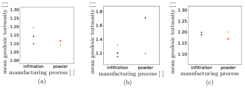
Figure 11: Mean geodesic tortuosity (a), mean geodesic tortuosity of paths starting from TPB (b) and dilated mean geodesic tortuosity with $r$ = $0.1\text{\,}\mathrm{\SIUnitSymbolMicro m}$ (c), for nickel (blue), GDC (red) and pores (yellow).

Last but not least, the spherical contact distances and chord lengths of the three phases, i.e., nickel, GDC and pores, have been analyzed to investigate the impact of the manufacturing process on the 3D morphology of SOFC anodes. For the nickel phase, the cumulative distribution function values of spherical contact distances are lower for powder technology than for infiltration, see Figure 12a, which indicates a refined nickel phase structure for infiltration. Additionally, infiltration leads to lower cumulative probabilities for chord lengths than the powder technology, indicating a more elongated nickel phase structure for infiltration, see Figure 12b. For GDC and pores, only minor differences are observed in the spherical contact distance distributions of the two manufacturing processes. However, infiltration leads to lower cumulative probabilities of chord lengths for both phases, GDC and pores, compared to powder technology.

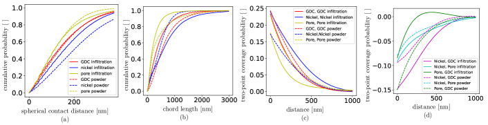
Figure 12: Cumulative distribution functions of spherical contact distance (a) and chord length (b) for nickel (blue), GDC (red) and pores (yellow), as well as centered two-point coverage probability functions for each of these phases (c) and for combinations of different phases (d).

The two-point coverage probabilities of both, GDC and pores, are larger for powder technology than for infiltration, while the opposite can be observed for the nickel phase, see Figure 12c. Moreover, the two-point coverage probabilities of the pore-GDC combination are significantly larger for infiltration than for the powder technology. For the remaining phase combinations, the powder technology leads to lower two-point coverage probabilities, see Figure 12d.

5 Conclusion

In the present paper, FIB-SEM image data have been used to analyze the 3D morphology of seven SOFC anodes, comprising of nickel, GDC and pore space. For this purpose, various geometric descriptors such as volume fraction, SSA, specific length of TPB and three different types of mean geodesic tortuosity have been computed. Besides the computation of these descriptors for each entire sample, their local heterogeneity is quantified by determining the distributions of local geometrical descriptors based on non-overlapping cutouts. This data enables the quantitative examination of the effect of various influencing factors (operating temperature, operating time and manufacturing process) on the resulting 3D morphology of SOFC anodes. It is shown that all three influencing factors mentioned above affect the anode morphology. In particular, when comparing the two manufacturing processes, powder technology and infiltration, it is noticeable that the volume fractions of the three phases (nickel, GDC, pores) and the specific length of TPB differ strongly from each other. Moreover, the higher operating temperature of $900\text{\,}\mathrm{\SIUnitSymbolCelsius}$ leads to a coarsening of the pore space. Similar effects can be observed with respect to operating time, where it is noticeable that the specific length of TPB significantly decreases with increasing operating time.

In a forthcoming study, the structural changes of SOFC anodes considered in the present paper will be modeled stochastically. In particular, a suitable spatial stochastic model will be determined, whose parameters will be calibrated to 3D image data of SOFC anodes for various operating times. Furthermore, by interpolation within the parameter space, it will be possible to carry out fast predictive simulations of SOFC anodes for operating times for which no image data is available. In this way, an efficient method will be established in order to provide the geometry input for spatially resolved numerical simulations of effective macroscopic properties. This will allow for efficient virtual testing of SOFC anodes, including the derivation of quantitative process-structure-property relationships.

References

- [1] A. Weber, Fuel flexibility of solid oxide fuel cells, Fuel Cells 21 (5) (2021) 440–452.
- [2] K. Kendall, M. Kendall, High-Temperature Solid Oxide Fuel Cells for the 21st Century: Fundamentals, Design and Applications, Academic Press, 2015.
- [3] J. Fergus, R. Hui, X. Li, D. Wilkinson, J. Zhang, Solid Oxide Fuel Cells: Materials Properties and Performance, CRC Press, 2016.
- [4] N. Brandon, E. Ruiz-Trejo, P. Boldrin, Solid Oxide Fuel Cell Lifetime and Reliability: Critical Challenges in Fuel Cells, Academic Press, 2017.
- [5] M. Singh, D. Zappa, E. Comini, Solid oxide fuel cell: Decade of progress, future perspectives and challenges, International Journal of Hydrogen Energy 46 (54) (2021) 27643–27674.
- [6] S. Zarabi Golkhatmi, M. I. Asghar, P. D. Lund, A review on solid oxide fuel cell durability: Latest progress, mechanisms, and study tools, Renewable and Sustainable Energy Reviews 161 (2022) 112339.
- [7] J. Zhang, C. Lenser, N. H. Menzler, O. Guillon, Comparison of solid oxide fuel cell (sofc) electrolyte materials for operation at , Solid State Ionics 344 (2020) 115138.
- [8] W. C. Chueh, Y. Hao, W. Jung, S. M. Haile, High electrochemical activity of the oxide phase in model ceria–Pt and ceria–Ni composite anodes, Nature Materials 11 (2) (2012) 155–161.
- [9] A. Nenning, C. Bischof, J. Fleig, M. Bram, A. K. Opitz, The relation of microstructure, materials properties and impedance of sofc electrodes: A case study of Ni/GDC anodes, Energies 13 (4) (2020).
- [10] S. Hussain, L. Yangping, Review of solid oxide fuel cell materials: Cathode, anode, and electrolyte, Energy Transitions 4 (2) (2020) 113–126.
- [11] J. Szász, F. Wankmüller, V. Wilde, H. Störmer, D. Gerthsen, N. H. Menzler, E. Ivers-Tiffée, Nature and functionality of oxygen/cathode/electrolyte-interfaces in sofcs, ECS Transactions 66 (2) (2015) 79.
- [12] T. Suzuki, Z. Hasan, Y. Funahashi, T. Yamaguchi, Y. Fujishiro, M. Awano, Impact of anode microstructure on solid oxide fuel cells, Science 325 (5942) (2009) 852–855.
- [13] P. A. Connor, X. Yue, C. D. Savaniu, R. Price, G. Triantafyllou, M. Cassidy, G. Kerherve, D. J. Payne, R. C. Maher, L. F. Cohen, R. I. Tomov, B. A. Glowacki, R. V. Kumar, J. T. S. Irvine, Tailoring SOFC electrode microstructures for improved performance, Advanced Energy Materials 8 (23) (2018) 1800120.
- [14] O. M. Pecho, A. Mai, B. Münch, T. Hocker, R. J. Flatt, L. Holzer, 3D microstructure effects in Ni-YSZ anodes: Influence of TPB lengths on the electrochemical performance, Materials 8 (10) (2015) 7129–7144.
- [15] J. R. Wilson, W. Kobsiriphat, R. Mendoza, H.-Y. Chen, J. M. Hiller, D. J. Miller, K. Thornton, P. W. Voorhees, S. B. Adler, S. A. Barnett, Three-dimensional reconstruction of a solid-oxide fuel-cell anode, Nature Materials 5 (7) (2006) 541–544.
- [16] N. Vivet, S. Chupin, E. Estrade, A. Richard, S. Bonnamy, D. Rochais, E. Bruneton, Effect of Ni content in SOFC Ni-YSZ cermets: A three-dimensional study by FIB-SEM tomography, Journal of Power Sources 196 (23) (2011) 9989–9997.
- [17] M. Kishimoto, M. Lomberg, E. Ruiz-Trejo, N. P. Brandon, Numerical modeling of nickel-infiltrated gadolinium-doped ceria electrodes reconstructed with focused ion beam tomography, Electrochimica Acta 190 (2016) 178–185.
- [18] J. A. Taillon, C. Pellegrinelli, Y. Huang, E. D. Wachsman, L. G. Salamanca-Riba, Three dimensional microstructural characterization of cathode degradation in SOFCs using focused ion beam and SEM, ECS Transactions 61 (1) (2014) 109.
- [19] M. Meffert, F. Wankmüller, H. Störmer, A. Weber, P. Lupetin, E. Ivers-Tiffée, D. Gerthsen, Optimization of material contrast for efficient FIB-SEM tomography of solid oxide fuel cells, Fuel Cells 20 (5) (2020) 580–591.
- [20] R. Mahbub, T. Hsu, W. K. Epting, G. Nolan, Y. Lei, N. T. Nuhfer, R. B. Doane, H. W. Abernathy, G. A. Hackett, S. Litster, A. D. Rollett, P. A. Salvador, Quantifying morphological variability and operating evolution in SOFC anode microstructures, Journal of Power Sources 498 (2021) 229846.
- [21] W. K. Epting, Z. Mansley, D. B. Menasche, P. Kenesei, R. M. Suter, K. Gerdes, S. Litster, P. A. Salvador, Quantifying intermediate-frequency heterogeneities of SOFC electrodes using X-ray computed tomography, Journal of the American Ceramic Society 100 (5) (2017) 2232–2242.
- [22] T. Hsu, W. K. Epting, R. Mahbub, N. T. Nuhfer, S. Bhattacharya, Y. Lei, H. M. Miller, P. R. Ohodnicki, K. R. Gerdes, H. W. Abernathy, G. A. Hackett, A. D. Rollett, M. De Graef, S. Litster, P. A. Salvador, Mesoscale characterization of local property distributions in heterogeneous electrodes, Journal of Power Sources 386 (2018) 1–9.
- [23] Y. Liu, F. Wankmüller, T. P. Lehnert, M. Juckel, N. H. Menzler, A. Weber, Microstructural changes in nickel-ceria fuel electrodes at elevated temperature, Fuel Cells 23 (6) (2023) 430–441.
- [24] Y. Liu, M. Juckel, N. H. Menzler, A. Weber, Ni/GDC fuel electrode for low-temperature SOFC and its aging behavior under accelerated stress, Journal of The Electrochemical Society 171 (5) (2024) 054514.
- [25] P. Getreuer, Rudin-Osher-Fatemi total variation denoising using split Bregman, Image Processing On Line 2 (2012) 74–95.
- [26] D. Kroon, Numerical optimization of kernel based derivatives, short paper, University Twente (2009).
- [27] E. Meijering, M. Jacob, J.-C. Sarria, P. Steiner, H. Hirling, M. Unser, Design and validation of a tool for neurite tracing and analysis in fluorescence microscopy images, Cytometry Part A 58A (2) (2004) 167–176.
- [28] S. Beucher, F. Meyer, The morphological approach to segmentation: The watershed transformation, in: E. R. Dougherty (Ed.), Mathematical Morphology in Image Processing, Marcel Dekker Inc., 1993, pp. 433–481.
- [29] I. Molchanov, Theory of Random Sets, Springer, 2005.
- [30] S. N. Chiu, D. Stoyan, W. S. Kendall, J. Mecke, Stochastic Geometry and its Applications, 3rd Edition, J. Wiley & Sons, 2013.
- [31] K. Schladitz, J. Ohser, W. Nagel, Measuring intrinsic volumes in digital 3D images, in: A. Kuba, L. Nyúl, K. Palágyi (Eds.), 13th International Conference Discrete Geometry for Computer Imagery, 2007, pp. 247–258.
- [32] L. Holzer, P. Marmet, A. Wiegmann, M. Neumann, V. Schmidt, Tortuosity and Microstructure Effects in Porous Media: Classical Theories, Empirical Data and Modern Methods, Springer, 2023.
- [33] M. Neumann, C. Hirsch, J. Staněk, V. Beneš, V. Schmidt, Estimation of geodesic tortuosity and constrictivity in stationary random closed sets, Scandinavian Journal of Statistics 46 (3) (2019) 848–884.
- [34] D. Jungnickel, Graphs, Networks and Algorithms, 3rd Edition, Springer, 2007.
- [35] B. Münch, L. Holzer, Contradicting geometrical concepts in pore size analysis attained with electron microscopy and mercury intrusion, Journal of the American Ceramic Society 91 (12) (2008) 4059–4067.
- [36] J. Serra, Image Analysis and Mathematical Morphology, Academic Press, 1982.
- [37] P. Soille, Morphological Image Analysis: Principles and Applications, 2nd Edition, Springer, 2003.
- [38] J. Ohser, K. Schladitz, 3D Images of Materials Structures: Processing and Analysis, Wiley-VCH, 2009.
- [39] J. Ohser, F. Mücklich, Statistical Analysis of Microstructures in Materials Science, J. Wiley & Sons, 2000.
- [40] J. Mayer, A time-optimal algorithm for the estimation of contact distribution functions of random closed sets, Image Analysis and Stereology 23 (2004) 177–183.