X

Efficient Eigenstate Preparation in an Integrable Model
with Hilbert Space Fragmentation

Roberto Ruiz^a†, Alejandro Sopena^a†, Balázs Pozsgay^b, Esperanza López^a

$\vphantom{x}{}^{a}$​ Instituto de Física Teórica UAM/CSIC
Universidad Autónoma de Madrid
C/ Nicolás Cabrera 13–15
Cantoblanco, 28049 Madrid, Spain

$\vphantom{x}{}^{b}$​ MTA-ELTE “Momentum” Integrable Quantum Dynamics Research Group,
ELTE Eötvös Loránd University
Pázmány Péter sétány 1/a,
1117 Budapest, Hungary

We consider the preparation of all the eigenstates of spin chains using quantum circuits. It is known that generic eigenstates of free-fermionic spin chains can be prepared with circuits whose depth grows only polynomially with the length of the chain and the number of particles. We show that the polynomial growth is also achievable for selected interacting models where the interaction between the particles is sufficiently simple. Our working example is the folded XXZ model, an integrable spin chain that exhibits Hilbert space fragmentation. We present the explicit quantum circuits that prepare arbitrary eigenstates of this model on an open chain efficiently. We perform error-mitigated noisy simulations with circuits of up to 13 qubits and different connectivities between qubits, achieving a relative error below 5%. As a byproduct, we extend a recent reformulation of the Bethe ansatz as a quantum circuit from closed to open boundary conditions.

1 Introduction

Eigenstate preparation is an important challenge in the application of quantum computation to the study of many-body physics. The implementation of eigenstates on a quantum computer would give direct access to their non-local properties, which are notably hard to obtain even resorting to tensor networks techniques, or to exact results for integrable systems. Moreover, eigenstates can be useful for benchmarking as well as the initialization of quantum algorithms.

Quantum circuits for eigenstate preparation must be efficient to be implementable, meaning that the number of one- and two-qubit gates must grow polynomially with the number of qubits and/or excitations in the model. There are efficient circuits that prepare free-fermion eigenstates exactly [1, 2, 3, 4, 5]. The existence of such algorithms relates to the fact free fermions are classically simulatable [6, 7, 8]. What is the class of models that admit efficient eigenstate preparation with unitary circuits remains an open question. It is true that ground states and certain excited states can have a relatively simple structure that enables efficient preparation. Conversely, our goal here is to develop algorithms capable of preparing arbitrary excited states in selected models.

It is natural to consider integrable spin chains with regard to this problem. Integrable systems are reputed to have simpler eigenstates than generic models, as integrability guarantees the models have completely elastic and factorized scattering processes [9]. The exact wavefunctions, which are computed by the coordinate Bethe Ansatz (CBA), are often known. The associated eigenstates can be usually constructed efficiently by a sequence of non-unitary linear operations, in a procedure known as algebraic Bethe Ansatz (ABA) [10, 11]. The search of a unitary counterpart of these protocols has attracted considerable attention in the recent years.

The paradigmatic spin chain solvable by the Bethe Ansatz is the XXZ model. Quantum circuits to prepare the eigenstates of the XXZ model with closed [12, 13, 14, 15] and open boundary conditions [16, 15] have been designed. They fall into two classes: probabilistic [12, 16] and deterministic algorithms [13, 14, 15]. The number of gates of the probabilistic algorithms in [12, 16] is polynomial in the number of qubits $N$ and excitations (“magnons”) $M$, but their success probability is exponentially small [17]. The number of gates of the deterministic algorithm of [15] is exponential in the number of magnons. Moreover, the deterministic circuits of [13, 14] involve multi-qubit unitaries, whose decomposition in terms of elementary gates likely suffers from the same problem. There are thus no known efficient quantum algorithm preparing the XXZ eigenstates. This raises the question of whether a quantum computer can access general eigenstates beyond those of free fermions. Our main result is proving that there are interacting many-body systems for which efficient algorithms prepare all their eigenstates.

Our strategy is to consider interacting models with relatively simple dynamical features. Specifically, we focus on the strong-coupling limit of the XXZ spin chain, where the dynamics drastically simplifies. There are essentially two ways to define an infinite-coupling limit of this spin chain, both of which can be understood as Schrieffer-Wolff transformation of certain kind. First, following [18], the model can be scaled to its triple point, which brings about the “constrained XX model”. The interactions of this spin chain consist of contact repulsion among magnons. The related but slightly different strong-coupling limit of [19, 20, 21] leads to the “folded XXZ model” [22, 23], whose excitations are magnons and domain walls. The Hilbert space of this spin chain splits into exponentially many subsectors with disconnected dynamics, which display the phenomenon called “Hilbert space fragmentation” [24, 25]. The folded XXZ model coincides with the constrained XX model in the purely magnonic sector. The simplicity of the folded XXZ model enabled exact computations in a variety of situations [21, 26, 27]. It is worth mentioning that the folded XXZ model has been realized experimentally in Rydberg atoms [28, 29].

In this paper, we construct a quantum circuit capable of preparing arbitrary eigenstates of the folded XXZ model with open boundaries exactly. The number of gates grows quadratically with the number of sites and linearly with that of excitations, being thus efficient. The structure of the circuit is the following. The initial state fed to the circuit is an $M$-magnon eigenstate of the free XX model. The first step is the application of a unitary $U_{0}$, which implements contact repulsion in such a way that the initial state is mapped onto an eigenstate of the constrained XX model. The output state then undergoes a second unitary $V_{D}$ which introduced the domain walls. Both $U_{0}$ and $V_{D}$ are built out of $\mathrm{CNOT}$ and $\mathrm{CSWAP}$. For the preparation of the XX eigenstates, we generalize the quantum algorithm of [13, 14], which prepare Bethe states on periodic chains, to open boundary conditions. We also perform numerical simulations of our circuits for several eigenstates with few excitations and sites. We consider different qubit connectivities and represent noise through a depolarizing channel.

The paper is organized as follows. In Section 2, we review the main properties of the folded XXZ model, explaining how Hilbert space fragmentation arises. In Section 3, we present the Bethe eigenstates of the model. In Section 4, we construct a quantum circuit whose input are eigenstates of the XX model and output those of the folded XXZ chain. In Section 5, we present numerical simulations of our quantum circuit. In Section 6, we conclude with general remarks and prospects on future research. Appendices A–D contain technical details.

2 The Folded XXZ Model

In this section, we introduce the folded XXZ model and discuss its main properties. The model is a spin-$1/2$ chain whose Hamiltonian is

$$H=-\frac{1}{8}\sum_{j}(1+\sigma^{z}_{j}\sigma^{z}_{j+3})(\sigma^{x}_{j+1}\sigma^{x}_{j+2}+\sigma^{y}_{j+1}\sigma^{y}_{j+2})\ .$$ (2.1)

The folded XXZ model is one of the simplest interacting spin chains. The model is integrable: it has an infinite family of local conserved charges. Furthermore, the model displays Hilbert space fragmentation. We discuss these properties below. We stress that there are models for discrete time evolution based on the folded XXZ model [30] that have been used in the analysis anomalous transport [31], but in this paper we consider only the Hamiltonian (2.1) and not the associated cellular automata.

The Hamiltonian density describes kinetically constrained hopping processes. If we identify spin-up and spin-down states with the computational basis of the qubit like

$$\ket{\uparrow}:=\ket{0}\ ,\quad\ket{\downarrow}:=\ket{1}\ ,$$ (2.2)

the processes allowed by (2.1) are

$$\ket{0100}\ \leftrightarrow\ \ket{0010}\ ,\quad\ket{1011}\ \leftrightarrow\ \ket{1101}\ .$$ (2.3)

We often use qubit rather than spin nomenclature. The Hamiltonian (2.1) clearly has two global $U(1)$ symmetries. The first corresponds to the charge

$$Q_{1}=\frac{1}{2}\sum_{j}(1-\sigma^{z}_{j})\ ,$$ (2.4)

which counts the number qubits at $\ket{1}$. The second corresponds to the charge

$$Q_{2}=\frac{1}{2}\sum_{j}(1-\sigma^{z}_{j}\sigma^{z}_{j+1})\ ,$$ (2.5)

which counts the number of changes from zero to one in a bit string. While both the Hamiltonian and $Q_{2}$ are invariant under a global bit flip. $Q_{1}\mapsto N/2-Q_{1}$ under this transformation instead.

The folded XXZ model can be derived from a special strong-coupling limit of the standard XXZ model with coupling constant $\Delta$, whose Hamiltonian is

$$H_{\mathrm{XXZ}}=\sum_{j}(\sigma^{x}_{j}\sigma^{x}_{j+1}+\sigma^{y}_{j}\sigma^{y}_{j+1}+\Delta\sigma^{z}_{j}\sigma^{z}_{j+1})\ .$$ (2.6)

The Hamiltonian (2.1) follows from both a Schrieffer-Wolff transformation at $\Delta\rightarrow\infty$ [19] and the $\Delta\rightarrow\infty$ limit of the fourth element of the family of local conserved charges of the Hamiltonian (2.6) [21]. Both approaches are regular at the level of the eigenstates. Therefore, all the eigenstates of the folded XXZ model match a $\Delta\to\infty$ limit of the eigenstates of the standard XXZ model. Furthermore, the existence of an infinite family of higher conserved charges follows from the $\Delta\to\infty$ limit of the family of the XXZ model [21].

The $\Delta\to\infty$ limit cannot be applied directly to the algebraic objects guaranteeing integrability. The Lax operators, the transfer matrices, and the R-matrices of the XXZ model are singular when $\Delta\to\infty$. New objects are needed to prove integrability in the framework of the Yang-Baxter equation [32]. The impediment implies that the construction of the eigenstates by the ABA can not be applied to the folded XXZ model directly. Furthermore, there is no obvious generalization.

However, it is possible to find all eigenstates of the folded XXZ model by means of the standard CBA, which uses linear superpositions of plane waves as trial functions. The applicability of the CBA was shown in the alternative approaches of [19] and [21], the latter of which we follow. Before we review the wavefunctions of the CBA in Section 3, we present the physics of the spin chain in this section. In Subsection 2.1, we describe the dynamical processes of the model. We then address the mechanism of Hilbert space fragmentation in Subsection 2.2.

2.1 The Dynamics of the Model

Physical processes of the folded XXZ model can be understood as the dynamics of isolated particles and holes together with domain walls. We define these concepts with the help of the computational basis first. We analyze transitions between states afterward.

We say that a transition is a link between two qubits such that two neighboring qubits carry different bits. Examples of states with transitions are $\ket{01}$ and $\ket{10}$. A particle is a single $\ket{1}$ embedded into a block $\ket{00\ldots 0}$, and a hole is a single $\ket{0}$ embedded into a block $\ket{11\ldots 1}$. For instance, $\ket{00100}$ has a particle at the third position and $\ket{11011}$ a hole at the third position. We use the common term “magnon” for both particles and holes. Magnons can be seen as a bound state of two transitions at neighboring positions. The state $\ket{0010011011}$ thus has two magnons: a particle on the third position and a hole on the eight position. Our definition implies that magnons cannot occupy neighboring positions, but they can occupy next-to-nearest neighboring positions. The position of magnons can be ambiguous in certain states. For example, we can say $\ket{1010}$ has two particles at the first and third position or two holes at the second and fourth positions. We resolve the ambiguity by choosing magnons to be at leftmost available configuration, hence $\ket{1010}$ has two particles rather than two holes.

A domain is a block of the spin chain with more than one qubit at the same state of the computational basis. The state $\ket{0011}$ then has two domains of length two. A domain wall is a transition between two domains. We do not count transitions associated to magnons as domain walls because domains have more than one qubit. We illustrate the identification of domain walls and magnons in a state in Fig. 1.

Figure 1: Example of identification of particles, holes, and domain walls. Particles appear in blue, holes in red, and straight vertical lines denote domain walls.

Much like the location of magnons themselves, the positions of domain walls is ill-defined if there are magnons in their immediate vicinity. For example, the state $\ket{001011}$ has one magnon and one domain wall, and we can say that the particle is at the third position and the domain wall between the fourth and the fifth position, or a hole at the fourth position and a domain wall between the second and the third position. We resolve the ambiguity by choosing magnons to be at the leftmost available position again. The state $\ket{001011}$ thus has a magnon at the third position and domain wall between the fourth and the fifth positions.

Magnons and domain walls allows us to discuss the basic physical dynamical processes of the model. The reason is that (2.3) can be seen as hopping terms for magnons. All magnons are separated by at least one position, and the kinetic term ensures that this constraint is kept during time evolution. Neither two particles nor two holes can jump to neighboring positions.

The states that do not have any domain walls from the “purely magnonic sector” of the Hilbert space. This sector splits into further subspaces according to the value of $Q_{1}$. The purely magnonic sector is the eigenspace with maximum $Q_{2}$ for given $Q_{1}$. Let $N$ denote the number of qubits (assumed to be even). The eigenspace with $Q_{1}=N/2$ has the maximal number $N/2$ of magnons. No state with domain walls belongs to the $Q_{1}=N/2$ sector, which has just two states, namely, the Néel state and the anti-Néel state. Both states are trivial eigenstates of (2.1) with zero energy. Purely magnonic sectors with $Q_{1}<N/2$ and $Q_{1}>N/2$ have non-maximal number of magnons. The eigenstates in this case are common to the constrained XX model, the parity-breaking variant of the folded XXZ model in purely magnonic sectors. This spin chain is the point $\Delta=0$ of the constrained XXZ model [33, 34, 35, 36], whose correlation functions have been the object to intensive research [37, 38, 39, 40]. We write the eigenstates of purely magnonic sectors in Subsection 3.1.

The crucial difference between the folded XXZ model and the constrained XX model, in addition to parity invariance, is that the former also allows domain walls in the Hilbert space. It follows from the kinetically constrained hopping (2.3) that isolated domain walls are frozen. For instance, the Hamiltonian annihilates the state $\ket{0011}$, which has an isolated domain wall in the middle. A domain wall only moves when it scatters with a magnon, resulting in the non-trivial dynamics of the model. Let us consider the example of the initial state $\ket{\psi}=\ket{001001111}$ and let us act with the Hamiltonian on top multiple times. At each step multiple hopping processes occur. One possible hopping sequence is

$$\begin{split}\ket{001001111}\quad\rightarrow\quad\ket{000101111}\quad\rightarrow\quad\ket{000110111}\quad\rightarrow\quad\ket{000111011}\ .\end{split}$$ (2.7)

We began with a state with a particle on the left and a single isolated and immobile domain wall. The hopping processes dragged the particle close to the domain wall. Since the particle could not reach the domain wall, it “transmuted” into a hole instead. (See [41] for an earlier analysis of such a phenomenon.) The transmutation of the particle into a hole moved the domain wall to the left by two positions. Such interactions happen whenever a magnon meets a domain wall, be it a particle or a hole. The scattering event leads to the displacement of the domain walls as well as the magnons. All the eigenstates can be understood by the interaction of magnons among them and with the domain walls that might be present.

2.2 Hilbert Space Fragmentation

The dynamical processes above lead to the phenomenon of Hilbert space fragmentation. Hilbert space fragmentation denotes the split of the Hilbert space splits into exponentially many subspaces, called fragments or sectors, such that all the entries of the Hamiltonian between different fragments vanish [24, 25]. The definition is physically meaningful if the fragments can be constructed via local constraints or local rules before actually finding all the exact eigenstates.

In the folded XXZ model, the fragmentation arises from the kinematic constraint in the hopping processes. Different fragments can be labeled by the numbers of magnons and the number and relative positions of the domain walls. The domain walls are not mobile on their own, thus their relative position does not change unless there is a scattering event with a magnon. This implies that, if one properly takes into account the displacements caused by the magnons, then one can uniquely label the fragments by the relative position of the domain walls.

We should mention that this description only applies to open boundary conditions. The mechanism of fragmentation is independent of the boundary conditions, but open boundary conditions enable simple labeling of the fragments. Such a labeling was introduced in [21, 42] using “effective coordinates” (alternative descriptions of fragmentation were provided earlier in [22]). To label the fragments, we follow the effective coordinates of [21, 42] closely.

Let us then set open boundary conditions, and let us choose a state $\ket{\psi}$ of the computational basis. The procedure to obtain the labeling is the following. First, we compute the action of the Hamiltonian on the state multiple times $H^{n}\ket{\psi}$. The result is the Krylov basis of the fragment of $\ket{\psi}$. If we expand $H^{n}\ket{\psi}$ into the computational basis, the number of terms of the Krylov basis typically increases with $n$. Our goal is to identify a distinguished state of the computational basis appearing at a large enough $n$ that can be used as a label of the fragment. To this aim, we consider all the possible hopping processes which arise from multiple actions of the Hamiltonian, and we focus on a selected direction of the hopping. We move in this way the magnons to their leftmost possible position inside $\ket{\psi}$. The result is the distinguished state we use to label the fragment, where magnons are tightly packed at the left boundary, occupying next-to-nearest neighboring positions, while the domain walls remain somewhere else in the spin chain.

We illustrate the procedure with an example. We consider the initial state

$$\ket{0001001110111},$$ (2.8)

which includes two magnons (one particle and one hole), and one domain wall in the middle. First, we move the particle on the left side to its leftmost position by applying two hopping processes and obtain

$$\ket{0100001110111}\ .$$ (2.9)

We now move the hole on the right side to the left, transmuting in doing so the hole into a particle and shifting the domain wall in the middle. The result is the state

$$\ket{\Psi_{\mathrm{label}}}=\ket{0101000011111}\ ,$$ (2.10)

which we use as the label of the given fragment. Magnons are packed at the left boundary in this state, while a single domain wall is left in the chain.

Given the number of magnons of a sector, we can use the number and the positions of the domain walls in the distinguished state as a label of the fragment. Indeed, it follows from the procedure that the final positions of the magnons and the domain wall are uniquely defined. There are exponentially many possibilities for the labels for a given the number magnons and domain walls as per the freedom in placing the domain walls. This multiplicity that lies at the core of the Hilbert space fragmentation into exponentially many sectors. Note that magnons in the state that labels fragments are particles if $Q_{1}<N/2$ and holes if $Q_{1}>N/2$. (If $N$ is even, the pair of eigenspaces with $Q_{1}=N/2$ are one-dimensional and the labeling is trivial as we have already mentioned.)

It is important to emphasize that the mechanism of fragmentation is not related to the integrability of the model. For example, the addition of any sort of non-integrable diagonal perturbation would preserve the kinetic constraint of the hopping and thus fragmentation. Such perturbations were in fact addressed in [43, 44]. Furthermore, [43] showed that there is a large non-Abelian symmetry algebra associated with this special type of Hilbert space fragmentation, and that the symmetry algebra is generated by matrix-product operators with fixed bond dimension [43], and that this symmetry of matrix-product operators is compatible even with selected non-integrable perturbations. We do not use these properties here.

3 Eigenstates

In this section, we present the spectrum of the folded XXZ model on a chain with open boundaries. We focus on open boundary conditions because the behavior of domain walls in this case is simpler than for periodic chains. The labeling of fragments is in fact reflective of the simplicity and will be crucial for the construction of the quantum circuit. We consider an open spin chain composed of $N+2$ qubits labeled by $j=0,\ldots,N+1$. The Hamiltonian

$$H=-\frac{1}{8}\sum_{j=0}^{N-2}(1+\sigma^{z}_{j}\sigma^{z}_{j+3})(\sigma^{x}_{j+1}\sigma^{x}_{j+2}+\sigma^{y}_{j+1}\sigma^{y}_{j+2})\ ,$$ (3.1)

acts diagonally on the boundary qubits at positions $j=0$ and $j=N+1$, as it is clear from the allowed dynamical processes (2.3). Therefore, boundary qubits carry well-defined quantum numbers and the Hilbert space splits into four sectors depending on the states of these boundary qubits. The global bit-flip symmetry of the Hamiltonian implies that we can fix the qubit at position $j=0$ to be in $|0\rangle$.

As we explained in Subsection 2.2, the Hilbert space fragments of an open chain can be labeled by the state of the computational basis where magnons are at their leftmost positions and domain walls lie to their right. If the last qubit of the chain is in $|1\rangle$, the reference state of a fragment in this sector is

$$|0\,i_{1}\dots i_{N-1}11\rangle\hskip 28.45274pt{\rm or}\hskip 28.45274pt|0\,i_{1}\dots i_{N-2}001\rangle\ .$$ (3.2)

By using the transition rules (2.3) again, it is simple to see that the fragment associated to the first state is isomorphic to the fragment of a chain with $N+3$ qubits and reference state

$$|0\,i_{1}\dots i_{N-1}110\rangle\ .$$ (3.3)

The same argument implies that the fragment labeled by the second state is isomorphic to that of a chain with $N+1$ qubits and reference state

$$|0\,i_{1}\dots i_{N-2}00\rangle\ .$$ (3.4)

Hence, without loss of generality, we just consider below the sector where both boundary qubits are in $|0\rangle$.

We consider in the following that states of the form

$$|0\,i_{1}\dots i_{N-2}110\rangle\ ,\hskip 28.45274pt|011\,i_{3}\dots i_{N}0\rangle\ ,$$ (3.5)

contain a domain wall between the next to last and last qubit, and the first and second qubit respectively, even though the definition of domain wall of Subsection 2.1 does not encompass these cases. This guarantees that the number of domain walls in all the states of a fragment is the same. Moreover, it helps to establish a map between the eigenstates of the free XX model and those of the folded XXZ chain which will be the basis for our characterization of the latter.

With the previous small change in nomenclature, we describe now folded XXZ eigenstates of the form $|0\rangle\otimes|\Psi_{M,D}\rangle\otimes|0\rangle$, which carries $M$ magnons and $D$ domain walls. We will show below that the state $|\Psi_{M,D}\rangle$, describing the central $N$ spins, can be written as

$$|\Psi_{M,D}\rangle=U_{D}\Big{(}\,|\Phi_{M}\rangle_{N_{0}}\otimes|{0}\rangle^{\otimes N-N_{0}}\Big{)}\ ,$$ (3.6)

where $|\Phi_{M}\rangle$ is an $M$-magnon eigenstate of the XX model, realizing free spinless fermions, and $U_{D}$ is a unitary. The XX eigenstate lives on an open chain with a reduced number of sites $N_{0}=N+1-M-D$. Due to the reflection with the open boundaries, each magnon of the XX model has components with momenta $\pm p_{a}$, where

$$p_{a}={\frac{\pi m_{a}}{N_{0}+1}}\ ,\hskip 28.45274pt$$ (3.7)

and $m_{a}$, $a=1,\ldots,M$, are integers. The unitary operator $U_{D}$ introduces the contact repulsion among magnons and contains the information on the domain wall positions. It implements a collection of permutations and bit flips, but does not alter the value of the XX eigenstate coefficients. Therefore, the magnon momenta of the folded XXZ chain are directly inherited from those of $|\Phi_{M}\rangle$. The only effect of the interaction on the spectrum of allowed momenta is through $M$ and $D$ in the effective length $N_{0}$ in (3.7).

The formula (3.6) was not given in this form before. It is a convenient representation of the eigenstates because it directly leads to the circuits that prepare them: we prepare $|\Phi_{M}\rangle$ first, and afterward act with the circuit $U_{D}$ for which we provide the factorization into elementary gates. However, the key results behind formula (3.6) appear in earlier works, including the original work on the constrained XXZ model [33, 34], as well as in the more recent [21, 42], which treated the folded XXZ model as a “hard-rod deformation” of the XX spin chain.

3.1 Magnons

We briefly review purely magnonic eigenstates, which are common to the constrained XX model. Since we have chosen the boundary spins to be in $|0\rangle$, magnons correspond univocally to qubits in $|1\rangle$. For states containing a single magnon, the folded Hamiltonian on a chain of $N+2$ qubits reduces then to that of the XX model on the $N$ bulk qubits. Therefore, one-magnon eigenstates are $|\Psi_{1,0}\rangle=|\Phi_{1}\rangle$, where $|\Phi_{1}\rangle$ is a plane wave with free open boundary conditions:

$$|\Phi_{1}\rangle=|\Phi(p)\rangle-|\Phi(-p)\rangle\ ,\hskip 28.45274pt|\Phi(p)\rangle=\sum_{n=1}^{N}\operatorname{e}^{\operatorname{i\!}pn}\sigma_{n}^{-}|{0}\rangle^{\otimes N}\ .$$ (3.8)

In this simple case, the unitary $U_{0}$ in (3.6) is just the identity.

The folded XXZ Hamiltonian (3.1) induces free open boundary conditions on the bulk qubits also for states with a general number of magnons. Generalizing (3.8), this implies that $|\Psi_{M,0}\rangle$ will be given by

$$|\Psi_{M,0}\rangle=\sum_{\epsilon_{a}=\pm 1}\left[\,\prod_{b=1}^{M}\epsilon_{b}\right]|\Psi(\epsilon_{1}p_{1},\ldots,\epsilon_{M}p_{M})\rangle\ .$$ (3.9)

Each $|\Psi(p_{1},\ldots,p_{M})\rangle$ is a Bethe state, namely, a superposition of plane waves whose coefficients are determined by the two-body scattering matrix, which for the folded XXZ model is

$$S(p_{1},p_{2})=-\operatorname{e}^{-\operatorname{i\!}\,(p_{1}-p_{2})}\ .$$ (3.10)

Although this scattering phase represents a non-trivial interaction, its effect amounts to shifting the coordinate dependence of the plane-wave factors such that

$$|\Psi(p_{1},\ldots,p_{M})\rangle=\!\!\!\sum_{1\leq n_{1}<\ldots<n_{M}\leq N}\Phi(n_{1},n_{2}\!-\!1,\ldots,n_{M}\!-\!M\!+\!1)\ |n_{1}n_{2}\ldots n_{M}\rangle\ ,$$ (3.11)

where $\Phi(n_{1},\ldots,n_{M})$ is the Slater determinant describing free-fermion wavefunctions

$$\Phi(n_{1},n_{2},\ldots,n_{M})=\begin{vmatrix}\operatorname{e}^{\operatorname{i\!}p_{1}n_{1}}&\operatorname{e}^{\operatorname{i\!}p_{1}n_{2}}&\ldots&\operatorname{e}^{\operatorname{i\!}p_{1}n_{M}}\\ \vdots&\vdots&\ddots&\vdots\\ \operatorname{e}^{\operatorname{i\!}p_{M}n_{1}}&\operatorname{e}^{\operatorname{i\!}p_{M}n_{2}}&\ldots&\operatorname{e}^{\operatorname{i\!}p_{M}n_{M}}\\ \end{vmatrix}\ .$$ (3.12)

We stress that (3.12) is nothing but the Bethe wavefunction of the CBA for the XX model. In (3.11) we have introduced the notation

$$|n_{1}n_{2}\ldots n_{M}\rangle=\,\sigma_{n_{1}}^{-}\sigma_{n_{2}}^{-}\ldots\sigma_{n_{M}}^{-}|0\rangle^{\otimes N}\ .$$ (3.13)

It is now immediate to define a unitary operation embedding the eigenstates of the XX model into the purely magnonic sector of the folded XXZ chain. According to (3.6), we search for a transformation $U_{0}$ such that

$$|\Psi(p_{1},\ldots,p_{M})\rangle=U_{0}\Big{(}|\Phi(p_{1},\ldots,p_{M})\rangle_{N_{0}}\otimes|{0}\rangle^{\otimes N-N_{0}}\Big{)}\ ,$$ (3.14)

where in the absence of domain walls $N_{0}=N-M+1$. From (3.11), $U_{0}$ should just shift the position of the free magnons by

$$n_{a}\mapsto n_{a}+a-1\ .$$ (3.15)

This mapping shows that the particles of the folded XXZ model behave as “hard rods”. In other words, particles, instead of occupying just one position, appear to have a finite length $\ell=2$. The shift in the coordinates takes into account the “accumulation” of the total length of the particles as counted from the left end of the spin chain. This coordinate transformation is well-known for the classical hard-rod gas; see, for example, [45]. In the case of the quantum spin chains, this interpretation was given, for instance, in [21, 42].

Substituting (3.14) into (3.9), we recover the relation (3.6) for purely magnonic states. Consistently, the Bethe equations for the folded XXZ model on a chain with $N+2$ sites impose the same quantization condition on the magnon momenta as that of the XX model on $N_{0}$ sites (3.7). The states of both chains share the same energy

$$E=-2\sum_{a=1}^{M}\cos p_{a}\ .$$ (3.16)

3.2 One Magnon and Two Domain Walls

We construct eigenstates containing one magnon and two domain walls, since they already illustrate all the features of the interaction between magnons and domain walls. Our starting point will be the reference state labeling the chosen fragment of Hilbert space, $|\Psi_{\mathrm{label}}\rangle$. As explained in Section 2.2, the reference state contains the magnon at its leftmost position, which in this case is just the site at the position $j=1$:

$$|\Psi_{\mathrm{label}}\rangle=\sigma_{1}^{-}|\Psi_{0,2}\rangle\ .$$ (3.17)

The state $|\Psi_{0,2}\rangle$ describes the domain-wall positions. Let the left domain wall lies between the positions $d_{1}$ and $d_{1}+1$, and the right domain wall lies between the positions $d_{2}$ and $d_{2}+1$. Then

$$|\Psi_{0,2}\rangle=\prod_{j=d_{1}+1}^{d_{2}}\sigma_{j}^{-}\,|0\rangle^{\otimes N}\ ,$$ (3.18)

where necessarily $2\leq d_{1}<d_{2}\leq N$.

Starting from (3.17), the magnon behaves as a particle that propagates freely until position $d_{1}-1$, that is, until it faces the first domain wall. We denote the basis of available states to the left of the domain wall as

$$|\psi_{2}(n)\rangle_{\mathrm{LP}}=\sigma_{n}^{-}|\Psi_{0,2}\rangle\ .$$ (3.19)

The magnon cannot reach the position $d_{1}$ as a particle, since the transition rules (2.3) forbid the merger between a particle and a domain. This forces the magnon to transmute into a hole, a process that displaces the first domain wall two positions to the left, between positions $d_{1}-2$ and $d_{1}-1$. The magnon propagates then freely as a hole between $d_{1}+1\leq n\leq d_{2}-1$. We represent these configurations by

$$|\psi_{2}(n)\rangle_{\mathrm{H}}=\sigma_{d_{1}-1}^{-}\sigma_{d_{1}}^{-}\sigma_{n}^{+}|\Psi_{0,2}\rangle\ .$$ (3.20)

The magnon abandons the domain after the position $d_{2}-1$, turning into a particle again. This shifts the right domain wall to the position between the $d_{2}-2$ and $d_{2}-1$ sites. Finally, the magnon propagates freely between $d_{2}+1\leq n\leq N$. We represent the corresponding states by

$$|\psi_{2}(n)\rangle_{\mathrm{RP}}=\sigma_{d_{1}-1}^{-}\sigma_{d_{1}}^{-}\sigma_{d_{2}-1}^{+}\sigma_{d_{2}}^{+}\sigma_{n}^{-}|\Psi_{0,2}\rangle\ .$$ (3.21)

The magnon in summary propagates as a free spinless fermion, whose position receives additional shifts each time it scatters with a domain wall, in turn displaced as well.

According to the previous description, the eigenstates of one magnon and two domain walls break into three parts: the left particle, the hole, and the right particle. Explicitly,

$$|\Psi_{1,2}\rangle=|\Psi_{\mathrm{LP}}\rangle+|\Psi_{\mathrm{H}}\rangle+|\Psi_{\mathrm{RP}}\rangle\ .$$ (3.22)

Each term separately mimics the state (3.8) over a sub-chain:

$$\begin{split}&|\Psi_{\mathrm{LP}}\rangle=\sum_{n=1}^{d_{1}-1}\sum_{\epsilon=\pm 1}\epsilon\operatorname{e}^{\operatorname{i\!}\epsilon pn}|\psi_{2}(n)\rangle_{\mathrm{LP}}\ ,\\ &|\Psi_{\mathrm{H}}\rangle=\sum_{n=d_{1}}^{d_{2}-2}\sum_{\epsilon=\pm 1}\epsilon\operatorname{e}^{\operatorname{i\!}\epsilon pn}|\psi_{2}(n+1)\rangle_{\mathrm{H}}\ ,\\ &|\Psi_{\mathrm{RP}}\rangle=\sum_{n=d_{2}-1}^{N-2}\sum_{\epsilon=\pm 1}\epsilon\operatorname{e}^{\operatorname{i\!}\epsilon pn}|\psi_{2}(n+2)\rangle_{\mathrm{RP}}\ .\end{split}$$ (3.23)

The Bethe equations require the magnon momentum to satisfy

$$p=\frac{\pi m}{N-1}\ ,$$ (3.24)

with $m$ integer, which coincides with momentum quantization of a free spinless fermion propagating on an open chain of $N_{0}=N-2$ qubits. Domain walls carry no momenta since they are static but for scattering with magnons.

It is straightforward to define a unitary operator satisfying

$$|\Psi_{1,2}\rangle=U_{2}\Big{(}|\Phi_{1}\rangle_{N-2}\otimes|00\rangle\Big{)}\ ,$$ (3.25)

where $|\Phi_{1}\rangle$ is the plane wave (3.8). The operator $U_{2}$ knows about the position of domain walls in the reference state (3.17), and acts as follows

$$\sigma_{n}^{-}|0\rangle^{\otimes N-2}\;\;\;\longrightarrow\;\;\begin{cases}\;|\psi_{2}(n)\rangle_{\mathrm{LP}}\ ,&\hskip 11.38092pt1\leq n\leq d_{1}-1\ ,\\ \;|\psi_{2}(n+1)\rangle_{\mathrm{H}}\ ,&\hskip 11.38092ptd_{1}\leq n\leq d_{2}-2\ ,\\ \;|\psi_{2}(n+2)\rangle_{\mathrm{RP}}\ ,&\hskip 11.38092ptd_{2}-1\leq n\leq N-2\ .\end{cases}$$ (3.26)

The operator $U_{2}$ detects the position of the magnon on the shorter free chain with no domains, relocates the magnon into the physical chain containing two domain walls at their reference positions, and shifts the domain walls when required according to the rules (2.3). We close the analysis by stressing that the energy of the eigenstate (3.25) is again given by (3.16) with $M=1$. Domain walls correct the quantization of momenta, but do not affect the form of the dispersion relation.

3.3 $\bm{M}$ Magnons and $\bm{D}$ Domain Walls

Finally, we build eigenstates containing $M$ magnons and $D$ domain walls. These states combine the features of the interaction of magnons among themselves and with domain walls treated in the previous subsections.

As before, our starting point is the reference state labeling the fragment to which the eigenstate we want to prepare belongs, $|0\rangle\otimes|\Psi_{\mathrm{label}}\rangle\otimes|0\rangle$. This state packs the magnons to the left, taking into account that they cannot occupy neighboring positions, and thus reads

$$|\Psi_{\mathrm{label}}\rangle=\sigma_{1}^{-}\sigma_{3}^{-}\ldots\sigma_{2M-1}^{-}|\Psi_{0,D}\rangle\ .$$ (3.27)

The state $|\Psi_{0,D}\rangle$ carries the domain walls at their rightmost positions. The number of domain walls is always even because boundary qubits are at $\ket{0}$. Let the first domain wall lie between the positions $d_{1}$ and $d_{1}+1$, where necessarily $d_{1}>2M$, the second between $d_{2}$ and $d_{2}+1$, and so on. The domain walls reference state reads

$$|\Psi_{0,D}\rangle=\left[\prod_{j_{1}={d_{1}+1}}^{d_{2}}\sigma_{j_{1}}^{-}\right]\left[\prod_{j_{2}={d_{3}+1}}^{d_{4}}\sigma_{j_{2}}^{-}\right]\ldots\left[\prod_{j_{D/2}=d_{D-1}+1}^{d_{D}}\sigma_{j_{D/2}}^{-}\right]|0\rangle^{\otimes N}\ .$$ (3.28)

The dynamical connection between the state that labels the fragment and other configurations parallels the simple case addressed in the previous subsection. The only new constraint is the contact repulsion among magnons. We illustrate the situation with an example. Let us assume the rightmost $L$ magnons are inside the (large enough) domain that lies between position $d_{K}$ and $d_{K+1}$, with $K$ odd, while the remaining $M-L$ magnon still lie at their initial positions. The associated state is

$$\underbrace{\sigma_{1}^{-}\sigma_{3}^{-}\ldots\sigma_{2M-2L+1}^{-}}_{M-L\leavevmode\nobreak\ \text{particles}}\underbrace{\sigma_{d_{1}-2L}^{\,x}\sigma_{d_{1}-2L+1}^{\,x}\ldots\sigma_{d_{K}-2}^{\,x}\sigma_{d_{K}-1}^{\,x}}_{{K\leavevmode\nobreak\ \text{displaced domain walls}}}\underbrace{\sigma_{h_{1}}^{+}\sigma_{h_{2}}^{+}\ldots\sigma_{h_{L}}^{+}}_{L\leavevmode\nobreak\ \text{holes}}|\Psi_{0,D}\rangle\ ,$$ (3.29)

where the locations of the holes satisfy the criterion of contact repulsion $h_{i}<h_{i+1}-1$. We have used $\sigma^{\,x}_{j}$ to relocate domain walls since it correctly acts as $\sigma^{-}_{j}$ or $\sigma_{j}^{+}$ when shifting the beginning or end of a domain, respectively. The remaining configurations with particles, holes, and domains walls are analogous. Particles and holes are placed within domains, and domain walls shift according to the number of magnons that have crossed them.

Like for purely magnonic eigenstates, the wavefunction of generic eigenstates is a Slater determinant whose dependence on magnon positions is properly shifted. The folded XXZ magnons behave as hard rods with effective length two. The effective length that the magnons perceive is further shortened by the presence of the domain walls. As illustrated in (3.26), the transmutation between particles and holes each time a magnon encounters a domain wall entails an additional shift of magnons one step to the right of the initial position of the domain wall. For this reason, it is enough to define the free-fermionic seed eigenstate $|\Phi_{M}\rangle$ in (3.6) on a chain of length $N_{0}=N-M+1-D$. To obtain the circuit preparing folded XXZ eigenstates, we find convenient to split the operator $U_{D}$ into the product of $U_{0}$, which constructs a purely magnonic state, and $V_{D}$, which introduces the domain walls next. In other words,

$$|\Psi_{M,D}\rangle=U_{D}\Big{(}|\Phi_{M}\rangle_{N_{0}}\otimes|0\rangle^{\otimes N-N_{0}}\Big{)}=V_{D}\Big{(}|\Psi_{M,0}\rangle_{N-D}\otimes|0\rangle^{\otimes D}\Big{)}\ .$$ (3.30)

Given a component $|n_{1}n_{2}\dots n_{M}\rangle$ of the state $|\Psi_{M,0}\rangle$, the unitary $V_{D}$ acts in the following iterative way. First, we focus on the rightmost qubit in $|1\rangle$, at position $n_{M}$. The action of $V_{D}$ is the insertion of a magnon in the state with domain walls like

$$|\psi_{D}(n_{M})\rangle=\left[\prod_{a=1}^{k_{M}}\sigma_{d_{a}-1}^{\,x}\sigma_{d_{a}}^{\,x}\right]\sigma^{\,x}_{n_{M}+k_{M}}|\Psi_{0,D}\rangle\ ,$$ (3.31)

where

$$\begin{array}[]{ll}k_{M}=0\ ,&\hskip 11.38109ptn_{M}<d_{1}\ ,\\ k_{M}=a\ ,&\hskip 11.38109ptd_{a}<n_{M}+a<d_{a+1}\ ,\\ k_{M}=D\ ,&\hskip 11.38109ptd_{D}<n_{M}+D\ .\end{array}$$ (3.32)

The particle at the position $n_{M}$ in the magnonic state moves to position $n_{M}+k_{M}$ in the presence of the domain walls, remaining a particle if $k_{M}$ is even and transmuting into a hole if $k_{M}$ is odd. At the same time, the domain walls shift by $d_{a}\mapsto d_{a}-2$ for $a\leq k_{M}$ and stay at their original positions otherwise. Next, $V_{D}$ inserts the particle of the purely magnonic state at position $n_{M-1}$ according to (3.31) again, but with $|\Psi_{0,D}\rangle$ replaced by $|\psi_{D}(n_{M})\rangle$. This step generates a new state $|\psi_{D}(n_{M-1},n_{M})\rangle$, in which the displacement $k_{M-1}$ is determined by (3.32) with respect to the new positions of the domain walls. The unitary $V_{D}$ iterates the process until $|\psi_{D}(n_{1},\dots,n_{M})\rangle$ is obtained. Analogously to (3.11), the eigenstates in the fragment correspond to the superposition

$$|\Psi_{M,D}\rangle=\sum_{\epsilon_{a}=\pm 1}\left[\,\prod_{b=1}^{M}\epsilon_{b}\right]|\Psi_{D}(\epsilon_{1}p_{1},\ldots,\epsilon_{M}p_{M})\rangle\ ,$$ (3.33)

with

$$|\Psi_{D}(p_{1},\ldots,p_{M})\rangle=\!\!\!\sum_{1\leq n_{1}<\ldots<n_{M}\leq N}\Phi(n_{1},n_{2}\!-\!1,\ldots,n_{M}\!-\!M\!+\!1)\,|\psi_{D}(n_{1},n_{2},\ldots,n_{M})\rangle\ ,$$ (3.34)

and $\Phi(n_{1},\dots,n_{M})$ the Slater determinant (3.12). The energy is given by (3.16)

4 The Quantum Algorithm

In this section, we build quantum circuits that efficiently prepare arbitrary eigenstates of the folded XXZ model. Following (3.6) and (3.30), the circuits consist of three parts. The first part builds eigenstates of the XX model with free open boundaries. The second transforms the eigenstates of the XX model into purely magnonic states of the folded XXZ chain. This part realizes the unitary $U_{0}$ defined in Subsection 3.1. Finally, the third part implements the unitary $V_{D}$ introduced in Subsection 3.3, which adds domain walls at the appropriate positions.

4.1 Algebraic Bethe Circuits with Open Boundary Conditions

Several quantum circuits to efficiently prepare free-fermion eigenstates are available in the literature [1, 2, 3, 4, 5]. In this paper, we elaborate on the recent proposal of [13, 14]. These works succeeded to recast the Bethe Ansatz in terms of quantum circuits, named “Algebraic Bethe Circuits (ABC)”. The growth of the computational resources required by ABC is linear in the number of qubits, but a priori exponential in the number of magnons. However, for the free XX model, the resources scale linearly both in the number of qubits and magnons, matching the efficiency of [2, 3]. The results of [13, 14] focused on preparing Bethe states on periodic chains. We show below that the construction easily generalizes to open boundary conditions.

It is well-known that the ABA [10, 11], which renders the underlying integrability explicit, can be reinterpreted in the language of matrix-product states (MPS) [46, 47, 48, 49, 50], the simplest example of one-dimensional tensor network [51]. It was shown in [14] that the CBA also admits a natural MPS formulation. According to [14], the plane-wave superposition of $M$ magnons on a closed chain of $N$ sites can be rewritten as

$$|\Psi(p_{1},\ldots,p_{M})\rangle=\operatorname{e}^{\operatorname{i\!}{\cal P}_{M}}\sum_{i_{j}=0,1}\langle 0|^{\otimes M}\Lambda^{i_{N}}\ldots\;\Lambda^{i_{1}}|1\rangle^{\otimes M}|i_{1}\dots i_{N}\rangle\ ,$$ (4.1)

where $\Lambda$ is the three-leg tensor characteristic of MPS formulations. Once the physical index $i$ is fixed, the tensor $\Lambda$ acts as a matrix on an auxiliary space, which for an $M$-magnon state has dimension $2^{M}$. Remarkably, the CBA tensor $\Lambda$ was obtained from a simple set of diagrammatic rules whose input are the magnon momenta and their associated scattering amplitudes. The normalization of the CBA wavefunctions in [14] slightly differs from the one here. The exponential of the total magnon momentum ${\cal P}_{M}$ in the right-hand side of (4.1) is the proportionality factor between both normalizations.

The CBA tensor can be seen as a $M\!+\!1$-qubit transformation $\bar{\Lambda}$ by identifying

$$\Lambda_{{\vec{\alpha}}{\vec{\beta}}}^{i_{k}}\equiv{\bar{\Lambda}}_{{\vec{\alpha}}0}^{i_{k}{\vec{\beta}}}=\langle i_{k}\,{\vec{\beta}}|{\bar{\Lambda}}|{\vec{\alpha}}\,0\rangle\ ,\quad$$ (4.2)

with ${\vec{\alpha}}=[\alpha_{1},\ldots,\alpha_{M}]$ and ${\vec{\beta}}=[\beta_{1},\ldots,\beta_{M}]$. We can then interpret (4.1) as a circuit with the staircase structure shown in Fig. 2(a), which acts on $N+M$ qubits initialized in the state $|1\rangle^{\otimes M}|0\rangle^{\otimes N-M}$. Nonetheless, there are two obvious problems with this interpretation. First, the $M$ rightmost output qubits should be postselected at $|0\rangle$ to obtain $|\Psi_{M}\rangle$, which implies an exponential shot cost in the number of magnons. Second, the “gates” $\bar{\Lambda}$ are not unitary. These issues can be addressed by using the large gauge freedom of the MPS [51]. The transformation

$$\Lambda^{i_{k}}\mapsto X_{k+1}\,\Lambda^{i_{k}}X^{-1}_{k}$$ (4.3)

where $X_{k}$ are arbitrary invertible matrices acting on the auxiliary space, together with

$$|1\rangle^{\otimes M}\mapsto X_{1}|1\rangle^{\otimes M}\ ,\hskip 28.45274pt\langle 0|^{\otimes M}\mapsto\langle 0|^{\otimes M}X_{N+1}^{-1}\ ,$$ (4.4)

leaves (4.1) invariant. If $X_{k}$ are chosen to preserve the $U(1)$ symmetry of the Bethe Ansatz, $|0\rangle^{\otimes M}$ and $|1\rangle^{\otimes M}$ remain invariant up to a factor. The freedom (4.3) allows us to transform an MPS into the so-called “canonical form” [51], such that

$${\bar{\Lambda}}_{{\vec{\alpha}}0}^{i_{k}{\vec{\beta}}}\mapsto(P_{N-k})_{{\vec{\alpha}}0}^{i_{k}{\vec{\beta}}}\ ,$$ (4.5)

with $P_{k}$ unitaries acting on qubits $M+1$. The new gates $P_{k}$ in general acquire a site dependence which breaks the translational invariance of the original MPS representation. 

The tensor $\Lambda$ building the $M$-magnon state satisfies the following property, which was central for the construction of (4.1):

$$|\Psi(p_{n_{1}},\ldots,p_{n_{r}})\rangle=\operatorname{e}^{\operatorname{i\!}{\cal P}_{r}}\sum_{i_{j}=0,1}\langle 0|^{\otimes M}\Lambda^{i_{N}}\ldots\;\Lambda^{i_{1}}|n_{1}\ldots n_{r}\rangle|i_{1}\ldots i_{N}\rangle\ ,$$ (4.6)

where the magnon momenta $p_{n_{a}}$ are chosen among the set $p_{1},\ldots,p_{M}$. Namely, the same tensor that builds an $M$-magnon state when the auxiliary qubits are initialized in $|1\rangle^{\otimes M}$ prepares Bethe states with $r<M$ magnons when the auxiliary qubits are initialized on an element of the computational basis with just $r$ qubits in $|1\rangle$. This property, together with the fact that $\Lambda$ does not depend on the number $N$ of physical sites, was crucial to explicitly determine the matrices $X_{k}$ that realize the transformation (4.5). The matrix $X_{k}$ orthonormalizes the states (4.6) on $k$ sites, for instance by the Gram-Schmidt process as illustrated in Fig. 3. Moreover, this automatically restricts the rank of the matrices $X_{k}$ for $k<M$, since the number of states of the form (4.6) exceeds the dimension of the corresponding Hilbert space. The unitaries $P_{k<M}$ act naturally on $k+1$ qubits, leading to the elimination of the ancilla of the MPS of the CBA. The resulting deterministic quantum circuit appears in Fig. 2(b). The $U(1)$ symmetry permits to fix the single-qubit gate $P_{0}$ as the identity and is thus discarded.

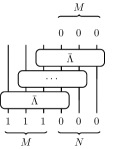
(a)

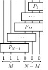
(b)

Figure 2: Realizations of Bethe states. Fig. 2(a) depicts the MPS of the CBA, whose $\bar{\Lambda}$ is non-unitary (rounded corners). Fig. 2(b) depicts ABC, where $P_{k}$ are unitaries (square corners).

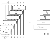
Figure 3: The matrix $X_{k+1}$ orthonormalizes the states of the CBA over $k$ sites, leading to a subcircuit with $N-k$ multi-qubit unitaries.

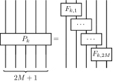
(a)

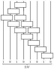
(b)

Figure 4: Unitaries of ABC with open boundary conditions at the free-fermion point. Fig. 4(a) depicts $P_{k}$ as a layer of gates of two-qubit gates $F_{k,a}$. Fig. 4(b) prepares the initial state of the $2M$ leftmost qubits of the open ABC circuit. It requires $\frac{1}{2}C(4M+1-3C)$ two-qubit gates, where $C=\lfloor(2M+1)/3\rfloor$.

It should be stressed that (4.6) builds Bethe states for arbitrary momenta, not necessarily satisfying the Bethe equations, which should be imposed separately. This fact in turn allows us to extend the previous construction to encompass the eigenstates of open chains. We focus on the XX model with free open boundaries in this subsection. We address interacting chains with open boundary conditions in Appendix A. The eigenstates of the open XX model with free open boundary conditions are given by

$$|\Phi_{M}\rangle=\sum_{\epsilon_{a}=\pm 1}\left[\,\prod_{b=1}^{M}\epsilon_{b}\right]|\Phi(\epsilon_{1}p_{1},\ldots,\epsilon_{M}p_{M})\rangle\ ,$$ (4.7)

where the right-hand side comprises Bethe states of the periodic XX model. To realize the superposition on the right-hand side of (4.7), we consider the tensor $\Lambda$ building a $2M$-magnon state with momenta $p_{1},-p_{1},\ldots.,p_{M},-p_{M}$. However, instead of initializing the MPS in the auxiliary space in $|1\rangle^{\otimes 2M}$, as in (4.1), or in an element of the computational basis of $2M$ qubits, as in (4.6), we choose the following product of $M$ entangled pairs

$$\underset{a=1}{\overset{2M}{\bigotimes}}\,{\big{(}\operatorname{e}^{\operatorname{i\!}p_{a}}|10\rangle-\operatorname{e}^{-\operatorname{i\!}p_{a}}|01\rangle\big{)}}\ .$$ (4.8)

The choice of an entangled initial state in the auxiliary space straightforwardly implies that the MPS network defined by $\Lambda$ outputs a superposition of Bethe states. The position of the qubits at $|1\rangle$ in the computational basis states expanding (4.8) determines, according to (4.6), which momenta appear in the associated Bethe state. The initial state (4.8) guarantees that none of the output Bethe states depends both on $p_{a}$ and $-p_{a}$. The relative sign between $|10\rangle$ and $|01\rangle$ takes care of the signs in the right-hand side of (4.7), while the factors $\operatorname{e}^{\pm\operatorname{i\!}p_{a}}$ build up the exponential of the total magnon momenta relating the MPS and CBA normalizations in (4.1).

Once we have completed the MPS construction, we turn into its conversion into a quantum circuit. We can achieve this task by transforming the tensor $\Lambda$ into canonical form using the MPS gauge freedom, like for closed chains. Since the open CBA tensor has to accommodate both $\pm p_{a}$, the resulting deterministic circuit is composed of quantum gates acting on up to $2M+1$ qubits, roughly twice the number needed for preparing the eigenstates of a closed chain. Specifically, the circuit to prepare an eigenstate with $N$ sites and $M$ magnons comprises $M(2N-2M-1)$ two-qubit gates and $2M-1$ single-qubit gates. However, this does not represent a significant increase in complexity for the XX model, whose $P_{k}$ gates were shown to efficiently decompose in terms of two-qubit unitaries as illustrated in Fig. 4(a). Analytic expressions for the single- and two-qubit unitaries can be found in Appendix B.

The MPS gauge freedom does not only require transforming the MPS tensors but, as shown in (4.4), the state in which the auxiliary qubits are initialized as well. While any $U(1)$-preserving action leaves the state with maximal $Q_{1}$ charge invariant up to a global factor, this is not the case for (4.8). Therefore, the initial state fed to the open ABC is

$$\rho X_{1}\left[\underset{a=1}{\overset{2M}{\bigotimes}}\,{\big{(}\operatorname{e}^{\operatorname{i\!}p_{a}}|10\rangle-\operatorname{e}^{-\operatorname{i\!}p_{a}}|01\rangle\big{)}}\right]\otimes|0\rangle^{\otimes N-2M}\ ,$$ (4.9)

where the constant $\rho$ ensures the state has unit norm. We have checked that the involved initial state of the $2M$ leftmost qubits can be reproduced efficiently by acting on the Néel state with the circuit of Fig. 4(b), whose two-qubit gates were determined numerically by optimization [52]. Although we do not address it here, we believe that an analytic expression for those gates is possible, as already obtained for the other elements composing the ABC of the XX model. This completes the preparation on a quantum computer of the eigenstates of the XX model with open boundary conditions.

4.2 From Free to Contact-Repulsive Magnons

We construct now a quantum circuit that maps XX eigenstates into purely magnonic eigenstates of the folded XXZ model, realizing the unitary $U_{0}$ we detailed in Subsection 3.1:

$$|\Psi_{M,0}\rangle=U_{0}\Big{(}\,|\Phi_{M}\rangle_{N-M+1}\otimes|{0}\rangle^{\otimes M-1}\Big{)}\ ,$$ (4.10)

This transformation introduces a contact repulsion among magnons by shifting free-magnon positions according to (3.15). Recall that we focus on folded XXZ eigenstates with the non-dynamical boundary spins at $|0\rangle$, such that $|\Psi_{M,0}\rangle$ denotes the state of the $N$ bulk spins of the chain. The qubit requirements of the circuit are the following.

• A physical register $R_{\mathrm{phys}}$ with $N$ qubits initialized in the state $|\Phi_{M}\rangle\otimes|{0}\rangle^{\otimes M-1}$.

• An auxiliary register $R_{\mathrm{aux}}$ with $M+1$ qubits initialized in $|1\rangle|0\rangle^{\otimes M}$, which keeps track of how many magnons have been already shifted.

The circuit searches for the free magnons in $|\Phi_{M}\rangle$ scanning from right to left. Every time a magnon is found, the qubit in $|1\rangle$ in $R_{\mathrm{aux}}$ moves one position toward the right. The concatenation of $\mathrm{CSWAP}$ gates of Fig. 5(a) performs this operation. We describe the action of the circuit on states of the computational basis. Consider that all operations associated to the scan from positions $N-M+1$ down to $n+1$ of $R_{\mathrm{phys}}$ have been already performed. The circuit focuses next on the $n$-th qubit, where we assume that the $r$-th magnon is placed. The module in Fig. 5(a) is executed with the $n$-th qubit as control. This places the $|1\rangle$ in $R_{\mathrm{aux}}$ at position $M-r+2$. The circuit now use the information in the auxiliary register to shift the $r$-the magnon according to (3.15), which is achieved by applying the module of Fig. 5(b) to the qubits $n$ to $n+M-1$ of $R_{\mathrm{phys}}$. Note that the action of this module is trivial if there is no magnon at position $n$.

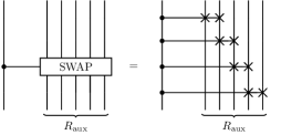
(a)

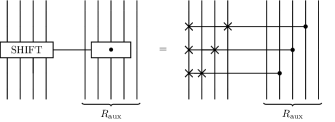
(b)

Figure 5: Building blocks of the circuit that implements the unitary $U_{0}$.

The iterating these operations leads us to the quantum circuit depicted in Fig. 6. Any $M$-magnon initial state leaves $R_{\mathrm{aux}}$ in the state $|0\rangle^{\otimes M}|1\rangle$ at the end of the circuit. This guarantees that physical and ancillary qubits end in a product state. Let us mention that the circuit in Fig. 6 admits straightforward simplifications that we have not included for the sake of clarity, since the modules in Figs. 5(a)–5(b) at the beginning and end of the circuit can only have a non-trivial effect on a reduced number of qubits.

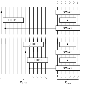
Figure 6: Circuit of the unitary $U_{0}$. It comprises fewer than $(2M\!-\!1)(N\!-\!M+1)$ $\mathrm{CSWAP}$ gates. For simplicity, we assume that all $\mathrm{CSWAP}$ gates act on $M+1$ qubits, which results in an overestimate of the total number of $\mathrm{CSWAP}$ gates.

4.3 Adding Domain Walls

A folded XXZ eigenstate with $D$ domain walls can be obtained by applying the unitary $V_{D}$ to the purely magnonic state $|\Psi_{M,0}\rangle$:

$$|\Psi_{M,D}\rangle=V_{D}\Big{(}|\Psi_{M,0}\rangle_{N-D}\otimes|0\rangle^{\otimes D}\Big{)}\ .$$ (4.11)

The unitary $V_{D}$ is defined by the shifting rules defined by (3.32). We explain a circuit implementation of $V_{D}$ that requires $2N+5$ qubits. The qubits are grouped as follows.

• A physical register $R_{\mathrm{phys}}$ with $N$ qubits initialized in the state $|\Psi_{0,D}\rangle$, which carries the domain walls at their positions in the reference state (3.28).

• An auxiliary register $R_{\mathrm{aux}}$ containing $N-D$ qubits initialized at the state $|\Psi_{M,0}\rangle$, which corresponds to the physical register of the previous subsection.

• A two-qubit register $R_{\mathrm{0}}$ initialized at $|0\rangle^{\otimes 2}$ used as workspace.

• A register $R_{\mathrm{c}}$ with $D/2+2$ qubits initialized in $|01\rangle|0\rangle^{\otimes{D/2}}$, which counts how many domain walls lie to the left of a given position in $R_{\mathrm{phys}}$.

• An additional $D/2+1$ register $R_{r}$ initialized at $|1\rangle|0\rangle^{\otimes{D/2}}$, which guarantees that $R_{\mathrm{phys}}$ is in a product state with any other registers of the circuit output.

The circuit deploys the magnons in $R_{\mathrm{aux}}$ successively, scanning from right to left, and inserts them into $R_{\mathrm{phys}}$, shifting along the way the domain walls according to the rules (3.32). We describe the action of the circuit when $R_{\mathrm{aux}}$ is initialized in a computational basis state compatible with the contact repulsion among magnons. Let us consider that all operations associated to the scan from the rightmost end to the $n+1$-th qubit of $R_{\mathrm{aux}}$ have been performed, and denote by $d_{1},\dots,d_{D}$ the positions of the domain walls in $R_{\mathrm{phys}}$ at this point. The focus turns then to the $n$-th position of the auxiliary register, $R_{\mathrm{aux},n}$. The tasks to be performed can be divided in three steps: moving the domain walls if a magnon is found at $R_{\mathrm{aux},n}$, inserting the magnon into $R_{\mathrm{phys}}$, and resetting the auxiliary qubits.

Moving the domain walls.

The basic element of the circuit that relocates the domain walls is the module shown in Fig. 7, which searches in the first block of qubits for $\ket{01}$ and $\ket{10}$ domain walls at positions 3 and 4 respectively, and moves them two sites toward the right depending on the state of a control qubit. If the control qubit is active, the 9-th qubit flips every time a domain wall is found, while the last $D/2+1$ qubits count the number of $|01\rangle$ domain walls. Recall that the presence of a magnon at $R_{\mathrm{aux},n}$ does not automatically trigger a shift of domain walls. Only those at positions $d_{1},\ldots,d_{k}$ must be shifted, where $k$ satisfies (3.32), that is,

$$d_{k}<n+k<d_{k+1}\ .$$ (4.12)

The control qubit should take care both of this condition and the state at $R_{\mathrm{aux},n}$.

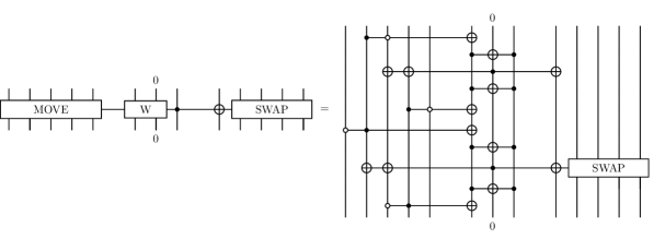
Figure 7: Module that shifts domain walls of the type $\ket{01}$ and $\ket{10}$.

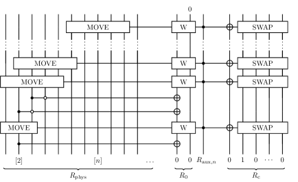
Figure 8: Circuit that shifts and counts domain walls starting from the first qubit in $R_{\mathrm{phys}}$ up to positions $n$ ($|01\rangle$) and $n+1$ ($|10\rangle$).

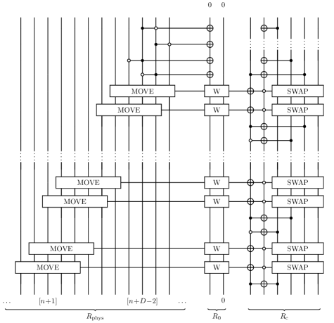
Figure 9: Circuit that completes the shift and count of domain walls by exploring up to $n+D$, the rightmost possible final position of the magnon.

The relocation of domain walls proceeds in two steps. In the first step, shown in Fig. 8, the circuit searches for $\ket{01}$ and $\ket{10}$ domain walls from the first qubit in $R_{\mathrm{phys}}$ up to positions $n$ and $n+1$ respectively. The domain walls encountered in this scan must be displaced if a magnon sits at $R_{\mathrm{aux},n}$, which hence is used as control for the gates defined in Fig. 7. The register $R_{\mathrm{c}}$ stores the information on the number of domain walls found, whose total number we denote by $k^{\prime}$. Condition (4.12) implies that $k^{\prime}=k$ only if $k^{\prime}\leq 1$. Otherwise the search for domain walls must be extended at least until the position $n+k^{\prime}$. If no further domain wall is found, (4.12) ensures that $k^{\prime}=k$ and the search stops. Alternatively the circuit updates $k^{\prime}$ to be the total number of domain walls up to that point, and iterates the previous operations. The circuit in Fig. 9 implements this scheme. Contrary to that in Fig. 8, it uses the second qubit of $R_{\mathrm{c}}$ as control for the shifting and counting of domain walls. This qubit is considered active at $|0\rangle$ instead of $|1\rangle$, which automatically ensures that there is a magnon at $R_{\mathrm{aux},n}$ and $k^{\prime}\geq 1$. It should be flipped from $|0\rangle$ to $|1\rangle$ when the $k$-th domain wall is reached. This is achieved by a series of Toffoli gates acting on the appropriate qubits of $R_{\mathrm{c}}$. At the end of the circuit, the second qubit of $R_{\mathrm{c}}$ is reset to its input state by a last Toffoli gate and a series of $\mathrm{CNOT}$s.

The operations performed by the module in Fig. 7 are carried out with the help of an ancillary workspace comprised of two qubits. This is symbolically represented by the gate W, a notation which we will keep using along this section. The working qubits are provided by the register $R_{\mathrm{0}}$. The second qubit of $R_{\mathrm{0}}$ resets to $|0\rangle$ after completion of the module in Fig. 7. Although it does not trigger any undesired operation, the first qubit does not reset in general when the control qubit is not active. This problem could be solved by adding two more Toffoli gates per module. A more resource-efficient solution is to have the first qubit return to $|0\rangle$ after the circuits of Figs. 8 and 9 have been completed. This is ensured by the $\mathrm{CNOT}$ and Toffoli gates at the beginning of Fig. 8 and the four Toffoli gates at the end of Fig. 9. These additional gates only play a role when the control is not active, forcing the concatenated MOVE gates to find every domain wall twice and thus flipping an even number of times the first qubit of $R_{\mathrm{0}}$.

Let us conclude with a remark on the circuit depicted in Fig. 8. Its first MOVE gate is centered in the second qubit of $R_{\mathrm{phys}}$. According to the pattern in Fig. 7, the leftmost qubit of this gate coincides with the left boundary qubit of the spin chain, which, being frozen at $|0\rangle$ by construction, has been omitted from $R_{\mathrm{phys}}$. The presence of a magnon at $R_{\mathrm{aux},n}$ forces any $\ket{10}$ domain wall to lie at $d\geq 4$, out of reach of the first MOVE gate, rendering thus the operations associated to the search for this type of domain wall irrelevant. As a result of these simplifications, the range of the first MOVE gate can be reduced from five to three qubits.

Inserting the magnon into $R_{\mathrm{phys}}$.

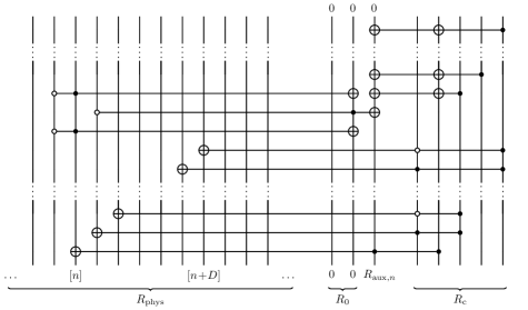
Figure 10: Circuit adding the magnons into $R_{\mathrm{phys}}$.

The circuits of Figs. 8 and 9 correctly relocate the domain walls according to the potential presence of a magnon in $R_{\mathrm{aux},n}$. The next step is to move the magnon, if present, from $R_{\mathrm{aux},n}$ into $R_{\mathrm{phys}}$ with the help of the information stored in $R_{\mathrm{c}}$. The circuit in Fig. 10 fulfills this task. The first chain of Toffoli gates duplicates the magnon and places the duplicate at the appropriate location in $R_{\mathrm{phys}}$. A further set of Toffoli gates resets $R_{\mathrm{aux},n}$ to $|0\rangle$.

Reset of ancillary qubits.

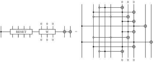
(a)

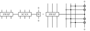
(b)

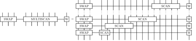
(c)

Figure 11: Building blocks of the reset circuit in Fig. 12. a) Search for a magnon as a hole at the third site or a magnon as a particle at the fourth, helped by the information in the first qubit. b) Search and count of domain walls at positions fourth and fifth. The number of qubits of the SCAN gate can vary; here we have chosen it to be three. c) Resource-efficient concatenation of the previous module.

At this point of the algorithm, the information stored in $R_{\mathrm{c}}$ is also contained in the position of the leftmost magnon in $R_{\mathrm{phys}}$. The circuit in Fig. 12 extracts this information directly from $R_{\mathrm{phys}}$ and uses it to reset $R_{c}$. Starting from the leftmost qubit of $R_{\mathrm{phys}}$, the circuit searches for $\ket{01}$ domain walls up to position $n-1$, and stores the result in a new register $R_{\mathrm{r}}$. Since two domain walls of this type cannot be separated by less than four sites, we can save resources as shown in Fig. 11(c), by applying the SCAN gate of Fig. 11(b) to concatenated blocks of five qubits. The first SCAN gate acts on the left boundary qubit, which has been omitted, together with the first $r+1$ qubits of $R_{\mathrm{phys}}$, where $r$ is the remainder of the quotient $(n-1)/4$.

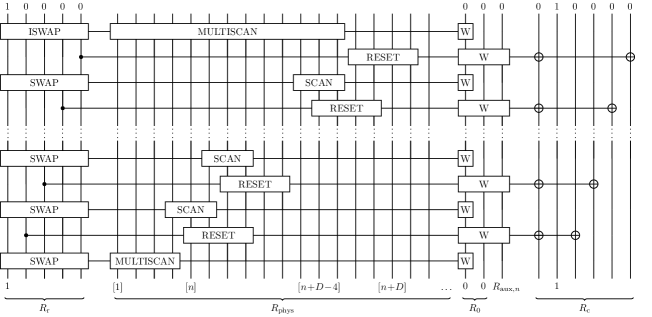
Figure 12: Circuit to reset the ancillary registers $R_{\mathrm{c}}$ and $R_{\mathrm{r}}$.

Let us assume that there was a magnon at $R_{\mathrm{aux},n}$. The circuit searches for this magnon from position $n+1$ to $n+D$ of $R_{\mathrm{phys}}$. The $n$-th position can be skipped because $R_{\mathrm{c}}$ keeps in its starting configuration when the magnon occupies it. First, the circuit queries whether there is a magnon in the form of a hole at site $n+1$ or a particle at $n+2$. A positive answer is not enough to ensure that the desired qubit has been found. For instance, the configuration $\ket{0010}$ on sites $(n,\!..,n+3)$ is also compatible with having encountered a previous magnon. According to the shifting rules (3.32), the situation of interest and the spurious one correspond respectively to having one and zero domain walls of type $|01\rangle$ to the left of the magnon. The module in Fig. 11(a) is able to discriminate between both situations using the information in the register $R_{\mathrm{r}}$.

The series of concatenated SCAN and RESET gates in Fig. 12 allows to unambiguously identify where the magnon was inserted and correctly reset $R_{\mathrm{0}}$. It is important to notice that the SCAN gates will count now $\ket{01}$ configurations associated both to domain walls and magnons. This agnostic counting is fundamental for the final reset of the register $R_{\mathrm{r}}$. The design of the circuit is such that a $\ket{01}$ count originated by a magnon never leads to an active $R_{\mathrm{r}}$ control qubit in the RESET gates. Finally, following the same scheme of Fig. 11(c), a series of SCAN gates is applied from position $n+D-3$ to the first qubit of $R_{\mathrm{phys}}$. They trigger a chain of $\mathrm{CSWAP}$ gates inverse to that in Fig. 5(a), denoted as $\mathrm{ISWAP}$, ensuring the reset of $R_{\mathrm{r}}$ after their completion.

	$\mathrm{CNOT}$	Toffoli	$\mathrm{CSWAP}$
Figs. 8–9	$(N\!-\!D\!-\!1)(\frac{1}{2}D\!+\!3N\!-\!15)$	$(N\!-\!D\!-\!1)(5D\!+\!4N\!-\!17)$	$\frac{1}{4}(N\!-\!D\!-\!1)(2D^{2}\!-\!5D\!+\!N)$
Fig. 10	$(N\!-\!D)D\!+\!2$	$(N\!-\!D\!-\!1)(D\!+\!4)\!+\!D\!+\!2$	$0$
Fig. 12	6	$2(N^{2}\!-\!7N+5)\!+\!D(7N\!-\!9D\!+\!3)$	$\frac{1}{8}D(N^{2}\!+\!5N\!-\!DN\!-\!6D-6)$

Table 1: Number of $\mathrm{CNOT}$, Toffoli, and $\mathrm{CSWAP}$ required by the circuits constructing a folded XXZ eigenstate with $D$ domain walls out of a purely magnonic state on $N-D$ sites. Values in blue indicate upper bounds.

All the circuits just described are run again, taking now the position $n-1$ of $R_{\mathrm{phys}}$ as reference. We iterate this process until all magnons are depleted from $R_{\mathrm{aux}}$, which ends in the state $|0\rangle^{\otimes N-D}$, while $R_{\mathrm{phys}}$ outputs the desired state $|\Psi_{M,D}\rangle$. Table 1 shows the number of $\mathrm{CNOT}$, Toffoli and $\mathrm{CSWAP}$ gates required by these circuits. For simplicity, we have considered that all $\mathrm{SWAP}$ gates act on $D/2+1$ qubits, although this overestimates the number of $\mathrm{CSWAP}$s required. For example, the first $\mathrm{SWAP}$ gate in Fig. 8 can be replaced by a single $\mathrm{CSWAP}$ between the second and third qubit of $R_{\mathrm{c}}$. Table 1 gives thus an upper bound to their number. Counting the number of Toffoli gates in the circuit of Fig. 12 leads to a lengthy expression due to the structure of the MULTISCAN gate. The value listed in Table 1 is an upper estimate.

5 Numerical Simulation of the Quantum Algorithm with Noise

In this section, we perform noisy simulations of the circuits preparing simple eigenstates of the folded XXZ model. It is important to stress that the circuit constructed following the instructions in Subsections 4.2 and 4.3 is able to prepare eigenstates belonging to any fragment of Hilbert space containing a chosen number of magnons and domain walls. We consider eigenstates with one magnon and two domain walls in chains with $N=5$ and $N=6$ bulk sites, or equivalently, 7 and 8 sites including the non-dynamical boundary qubits. The reference states of the available fragments are

$$\begin{split}\begin{matrix}N=5:\quad\quad&|10110\rangle\ ,\ &|10111\rangle\ ,&|10011\rangle\ ,&&\\ N=6:\quad\quad&|101100\rangle\ ,&|101110\rangle\ ,&|101111\rangle\ ,&|100110\rangle\ ,&|100111\rangle\ .\end{matrix}\end{split}$$ (5.1)

For the $N=5$ chain, we select the reference state $|10110\rangle$ and the magnon momentum $p=\pi/4$, while for the $N=6$ chain we choose $|100110\rangle$ and $p=\pi/5$.

Eigenstates with only two domain walls allow for a simplified version of the counting and reset strategies. Moreover, gates at the beginning or end of the circuits often require less ancilla qubits. In the small chains we consider for simulation, these simplified gates represent are a large share of the total number. Respecting the general strategy, we have restructured accordingly the circuits to be simulated, shown in Fig. 13, in the search for the highest efficiency. They address first the search for the $|01\rangle$ domain wall, corresponding to the operations shadowed in red, and once completed they turn to the remaining $|10\rangle$ domain wall, with operations shadowed in green. The working register $R_{\mathrm{0}}$ has been reduced to a single qubit, which is reset after each use. For the $N=6$ eigenstate, this reduction requires partially using $R_{\mathrm{c}}$ as workspace. The register $R_{\mathrm{c}}$ counting domain walls can be realized with just two qubits, which switch from $|0\rangle$ to $|1\rangle$ when the first or second domain wall is encountered. This in turns allows to insert the magnon at the appropriate location of the physical register by means of CNOT instead of Toffoli gates, which have been shadowed in blue. Finally, $R_{\mathrm{c}}$ can be reset without the need to introduce an additional register $R_{\mathrm{r}}$, corresponding to the area shadowed in yellow. Our goal is to estimate the circuit’s performance on current noisy intermediate-scale quantum (NISQ) [53] devices. The simulations are performed using the Qibo package [54]. Both the programs and the data necessary to reproduce the results are available in [52]. For completeness, Appendix C describes how the state of $R_{\mathrm{phys}}$ evolves through the circuits 13, taking as input the different domain wall reference states in (5.1).

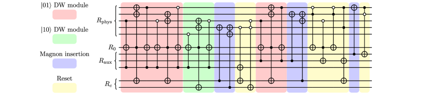
(a)

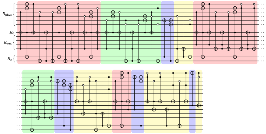
(b)

Figure 13: Circuit representation of $V_{D}$ used in the numerical simulations. Fig. 13(a) and Fig. 13(b) correspond to the circuits with $N=5$ and $N=6$, respectively.

The error rate of two-qubit gates is generally an order of magnitude higher than that of single-qubit gates on the main platforms, typically ranging from $10^{-4}$ to $10^{-3}$ [55, 56, 57, 58]. Therefore, we use a simplified noise model in which only the two-qubit gates are considered noisy. Coherent noise, which introduces systematic errors, can be transformed into incoherent noise through randomized compiling [59], as has been experimentally demonstrated on NISQ computers [60]. A simple model for incoherent noise is depolarizing noise. The $n$-qubit depolarizing channel is given by

$$\mathcal{E}(\rho)=(1-\lambda)\rho+\lambda\,\frac{\mathcal{I}}{2^{n}}\,,$$ (5.2)

where $\lambda$ is the depolarizing rate and $n$ is the number of qubits. We simulate a noisy two-qubit gate by applying a two-qubit depolarizing channel following the gate operation. This model characterizes a gate with error rate $r$ if $\lambda=(4r)/3$ [61]. According to the mentioned error rates, we choose a depolarizing parameter of $3\cdot 10^{-3}$.

Another important aspect to consider is the connectivity of the qubits, which significantly affects the fidelity of two-qubit gates, particularly between distant qubits. Current implementations of high-fidelity gates in superconducting quantum computers utilize static qubits arranged in a two-dimensional grid, which are generally restricted to nearest-neighbor connectivity [62]. In contrast, trapped-ion setups allow for the shuttling of qubits, enabling them to achieve all-to-all connectivity [63, 64, 65].

This consideration leads us to explore the scenario of all-to-all connectivity, where we decompose the circuit into $\mathrm{CNOT}$ gates and single-qubit gates, permitting connectivity between any pair of qubits. We also consider a scenario with more restricted connectivity, focusing specifically on the architecture of the Google Sycamore23 device [66], as shown in Fig. 14. To achieve this connectivity, a polynomial number of SWAP gates between connected qubits is necessary. It is important to find an optimal mapping between the qubits in our circuit and the physical qubits on the quantum device in order to minimize the number of SWAP gates. This problem, known as “routing”, is solved numerically using the SABRE algorithm [67], which is implemented in Qibo [54]. The number of $\mathrm{CNOT}$ gates, single-qubit gates, and the circuit depth is given in Table 2.

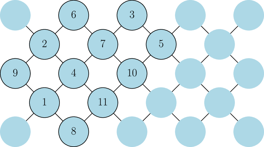
(a)

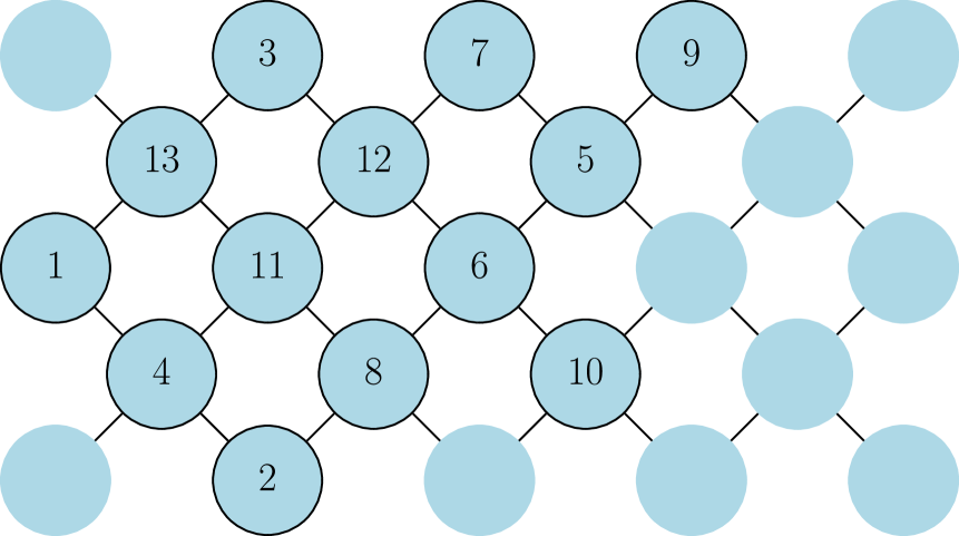
(b)

Figure 14: Mapping from virtual to physical qubits in the Sycamore23 quantum device. Fig. 14(a) corresponds to the state with $N=5$, where 11 physical qubits are used. Fig. 14(b) corresponds to the state with $N=6$, where 13 physical qubits are used. Among the 23 available qubits, the qubits we used are highlighted in black. Each number refers to a qubit in our circuit, ordered from top to bottom.

	N	$R_{Z}$	$R_{X}(\pi/2)$	$X$	$\mathrm{CNOT}$	Depth
All-to-all connectivity	5	$152$	$48$	$14$	$118$	$215$
	6	$392$	$98$	$32$	$316$	$448$
NN connectivity	5	$206$	$98$	$19$	$228$	$361$
	6	$501$	$194$	$42$	$639$	$795$

Table 2: Comparison of the number of quantum gates and circuit depth for all-to-all connectivity and nearest-neighbor (NN) connectivity for the circuits to prepare eigenstates with 5 and 6 bulk qubits.

To understand the impact of the noise, we simulate the state both with and without noise and calculate the fidelity between the two. The fidelity $F$ between two quantum states $\rho_{1}$ and $\rho_{2}$ is defined as

$$F(\rho_{1},\rho_{2})=\operatorname{tr}\left(\sqrt{\sqrt{\rho_{1}}\rho_{2}\sqrt{\rho_{1}}}\right)^{2}\,.$$ (5.3)

For the $N=5$ eigenstate, the fidelity is 0.7624 with all-to-all connectivity, but with nearest-neighbor connectivity, it drops to 0.5980. Similarly, the fidelity of the $N=6$ eigenstate decreases from 0.4841 with all-to-all connectivity to 0.2387 with nearest-neighbor connectivity. Additionally, we compute the energy of each eigenstate and the expectation values of the charges $Q_{1}$ and $Q_{2}$ under both conditions. It is important to note that these observables are defined over $N+2$ qubits. Given that the boundary qubits are in the state $|0\rangle$, we project these observables onto this subspace, enabling us to calculate them without simulating the entire states. The resulting values, along with their relative errors, are shown in Table 3.

	N	$\langle H\rangle$	$\langle Q_{1}\rangle$	$\langle Q_{2}\rangle$
Noiseless	5	$-0.7071$	$3$	$4$
	6	$-0.8090$	$3$	$4$
All-to-all connectivity	5	$-0.5363$ $(0.2415)$	$2.9085$ $(0.0305)$	$3.8442$ $(0.0389)$
		$-0.7124$ $(0.0075)$	$2.9743$ $(0.0086)$	$3.9969$ $(0.0008)$
	6	$-0.4103$ $(0.4929)$	$2.9249$ $(0.0250)$	$3.8078$ $(0.0481)$
		$-0.7786$ $(0.0376)$	$2.9753$ $(0.0082)$	$3.9272$ $(0.0182)$
NN connectivity	5	$-0.4215$ $(0.4039)$	$2.8409$ $(0.0530)$	$3.7126$ $(0.0719)$
		$-0.7249$ $(0.0251)$	$2.9597$ $(0.0134)$	$3.9426$ $(0.0144)$
	6	$-0.2102$ $(0.7402)$	$2.8950$ $(0.0350)$	$3.6791$ $(0.0802)$
		$-0.8209$ $(0.0146)$	$2.9355$ $(0.0215)$	$3.8440$ $(0.0390)$

Table 3: Summary of the simulated values for the energy $\langle H\rangle$ and the charges $\langle Q_{1}\rangle$, $\langle Q_{2}\rangle$, under noiseless and noisy conditions with all-to-all connectivity and nearest-neighbor (NN) connectivity with 5 and 6 bulk qubits. The second row for each number of qubits and connectivity represents the values after error mitigation, while the first row shows the noisy values. The relative errors with respect to the exact values are shown in parentheses for the noisy cases.

Clifford circuit data has been leveraged to reduce the impact of noise in quantum computations. Quantum circuits composed mainly of Clifford gates can be efficiently simulated on classical computers [68]. We utilize Clifford Data Regression (CDR) [69], an error mitigation technique where near-Clifford circuits are employed to generate a dataset of noisy and exact expectation values for a specific observable. This dataset is then used to train a simple linear model that maps noisy outcomes to their exact counterparts. Once trained, this model is applied to mitigate the noisy expectation values produced by circuits that cannot be efficiently simulated. For further details, refer to the Appendix D. The energy and the expectation values of the charges $Q_{1}$ and $Q_{2}$ after mitigation are shown in Table 3. Notably, CDR reduces the relative error of each observable by an order of magnitude.

6 Conclusions

In this paper, we constructed a quantum algorithm capable of preparing all the eigenstates of the folded XXZ model with open boundaries, containing both magnons and domain walls. To the best of our knowledge, it is the first efficient quantum algorithm that prepares every eigenstate of an interacting quantum spin chain. Along the way, we extended the reformulation of the Bethe ansatz in terms of quantum circuits, termed ABC in [13, 14], from closed to open chains.

The construction of the circuit relies on the description of eigenstates with magnons and domain walls of Section 3, which uses as seed an eigenstate of the XX model on a reduced number of sites. We proposed to prepare the XX eigenstate using the open boundary generalization of the ABC. The magnon contact repulsion is then implemented through the simple coordinate shift (3.15). Subsequently, the domain walls are displaced from their reference position following the rules (3.31) and (3.32), which automatically reveal whether a magnon is to be represented as a particle or a hole. Even though this picture is equivalent to the effective coordinates of [21, 42], it offers a simpler description of the folded XXZ eigenstates which could help to construct eigenstates of other models with similar dynamics.

Our circuits require ancillas, especially relevant to the eigenstates that have domain walls. To estimate the performance of circuits on NISQ computers, we ran numerical simulations including a simple depolarizing noise model. Since qubit connectivity has a strong impact on the fidelity of gates between distant qubits, we have considered two different architectures. First, an all-to-all connectivity, typical of trapped-ion and Rydberg-atom prototypes. Second, a square-lattice connectivity, as implemented in Google’s superconducting chips. Our simulations indicate that simple eigenstates, containing few magnons and domain walls, could be implemented with acceptable fidelity on quantum computers with two-qubit gate fidelity below $10^{-3}$. Therefore, our algorithm is a good candidate for benchmarking applications.

Hilbert space fragmentation [24, 25] has attracted much attention in recent years. The reason is that it describes a new type of ergodicity breakdown, hence of violation of the eigenstate thermalization hypothesis. Our results open the way to study of this phenomenon on a digital quantum computer, adding to previous proposals on a Rydberg-atom simulator [28, 29]. For example, it would be interesting to explore the evolution and mixing of folded XXZ fragments under perturbations of varying strength. One could use the fact that our algorithm allows preparing not only eigenstates, but also superpositions of eigenstates from different fragments. These superpositions can be easily implemented by initializing the physical register $R_{\mathrm{phys}}$ of the circuit in Subsection 4.3 in a superposition of reference-states $|\Psi_{0,D}\rangle$. The resulting output could then be fed to a quantum circuit realizing the Trotterized evolution under the desired perturbation.

Finally, it is clearly very interesting to search for other spin chain models whose spectrum can be efficiently prepared on a quantum computer. The circuits presented in this paper straightforwardly generalize to the class of constrained XX models of [70, 35, 71], in which contact repulsion among magnons extends to $\ell$ sites. Another class of interesting candidates are the recently found models of hidden free fermions [72, 73, 74]. Although these models seemingly display interaction, their Hamiltonians have a free-fermion spectrum. However, the associated fermionic operators do not follow from a Jordan-Wigner transformation. Notably, they admit Trotterizations compatible with the hidden free-fermion structure [75] that have been used to compute real-time dynamics [76]. These strong properties hint at the possibility that an efficient quantum circuit preparing their eigenstates could be also found.

Appendix A General Algebraic Bethe Circuits with Open Boundary Conditions

In this appendix, we supplement the presentation of ABC with open boundary conditions of Subsection 4.1. References [13, 14] proposed ABC, quantum circuits with multi-qubit unitaries. ABC prepare Bethe states of a spin-$1/2$ chain with periodic boundary conditions that preserve $U(1)$ symmetry. We adapt the framework of [13, 14] to open boundary conditions.

The cornerstone of ABC in [14] is the representation of Bethe states in the CBA as the translationally invariant MPS (4.1). The MPS appeared in [46, 47, 48], up to the normalization, but the connection with the CBA remained unnoticed. The elementary tensor of the MPS is $\Lambda$. To adjust $\Lambda$ to open boundary conditions, following Subsection 4.1, we treat incident and reflected plane waves of every single magnon independently. Let us define the set of $2M$ momenta

$$q_{2a-1}=p_{a}\ ,\quad q_{2a}^{\phantom{-1}}=-p_{a}\ ,\quad a=1,\ldots,M\ .$$ (A.1)

Let us also introduce the momenta variables

$$y_{a}=\exp(\operatorname{i\!}q_{a})\ ,$$ (A.2)

for later notational convenience. The scattering amplitude between the incident and reflected plane waves of $q_{a}$ with the plane wave of $q_{b}$ is $B(q_{a},q_{b})$. For instance, the scattering amplitude of the XXZ model with open boundary conditions is

$$B(q_{a},q_{b})=(1+y_{a}y_{b}-2\Delta y_{b})(1+y_{a}^{-1}y_{b}-2\Delta y_{a}^{-1})y_{b}^{-1}\ ,$$ (A.3)

where we recall $\Delta$ is the anisotropy. The tensor $\Lambda$ of ABC with open boundary conditions is shared with [14]. The tensor $\Lambda$ acts on $2M$ ancillary and produces one physical qubit in the state $|i\rangle$ and $2M$ ancillas, and reads 

$$\begin{split}\Lambda^{0}&=\bigotimes_{a=1}^{2M}\begin{bmatrix}1&0\\ 0&y_{a}\end{bmatrix}\ ,\quad\Lambda^{1}=\sum_{a=1}^{2M}\overset{a-1}{\underset{b=1}{\bigotimes}}\begin{bmatrix}1&0\\ 0&-B(q_{b},q_{a})y_{b}\end{bmatrix}\begin{bmatrix}0&1\\ 0&0\end{bmatrix}\overset{2M}{\underset{c=a+1}{\bigotimes}}\begin{bmatrix}1&0\\ 0&B(q_{c},q_{a})y_{c}\end{bmatrix}\ .\end{split}$$ (A.4)

Note $\Lambda$ is not unitary. We can use (4.1) to write

$$\begin{split}|\Psi(q_{n_{1}}\ldots,q_{n_{M}})\rangle=\operatorname{e}^{\operatorname{i\!}\mathcal{Q}_{a}}\sum_{i_{j}=0,1}\langle 0|^{\otimes 2M}\Lambda^{i_{N}}\ldots\;\Lambda^{i_{1}}|n_{1}\ldots n_{M}\rangle|i_{1}\ldots i_{N}\rangle\\ =\underset{1\leq\ell_{1}<\ldots<\ell_{M}\leq{N}}{\sum}\vphantom{\left[\sum_{\beta_{1},\ldots,\beta_{M}=1}^{2M}\right]}\sum_{\beta_{1},\ldots,\beta_{M}=1}^{M}\epsilon_{\beta_{1}\ldots\beta_{M}}\left[\underset{1\leq b<a\leq M}{\prod}B(\widetilde{q}_{\beta_{a}},\widetilde{q}_{\beta_{b}})\right]\vphantom{\left[\sum_{\beta_{1},\ldots,\beta_{M}=1}^{M}\right]}\left[\vphantom{\underset{1\leq a<b\leq M}{\prod}}\!\overset{M}{\underset{a=1}{\prod}}\,\,\widetilde{y}_{\beta_{a}}^{\,\ell_{a}}\right]\vphantom{\left[\sum_{\beta_{1},\ldots,\beta_{M}=1}^{M}\right]}\vphantom{\left[\sum_{\beta_{1},\ldots,\beta_{M}=1}^{M}\right]}|\ell_{1}\ldots\ell_{M}\rangle\ ,\end{split}$$ (A.5)

where

$$\operatorname{e}^{\operatorname{i\!}\mathcal{Q}_{a}}=\prod_{a=1}^{M}\operatorname{e}^{\operatorname{i\!}q_{n_{a}}}\ ,$$ (A.6)

$1\leq n_{1}<n_{2}<\ldots<n_{M}\leq 2M$ and we defined $\widetilde{q}_{a}:=q_{n_{a}}$ and $\widetilde{y}_{a}=y_{n_{a}}$. Therefore, (A.5) does not carry quasi-momenta $q_{2a}=p_{a}$ and $q_{2a-1}=-p_{a}$ at the same time as long as $n_{2a-1}\neq n_{2a}$.

Bethe states also compress self-scattering amplitudes if the boundaries are open. These amplitudes account for the interference between the incident and reflected plane waves of a single magnon. The self-scattering amplitude with quasi-momentum $q_{a}$ is $\alpha(q_{a})$. For instance, the self-scattering amplitude of the XXZ model with open boundary conditions in absence of boundary magnetic fields is

$$\alpha(q_{a})=1-\Delta y_{a}^{-1}\ .$$ (A.7)

The Bethe state of the CBA with open boundary conditions reads

$$|\Psi_{M}\rangle=\sum_{\epsilon_{a}=\pm 1}\left[\,\prod_{b=1}^{M}\epsilon_{b}\alpha(\epsilon_{b}p_{b})\right]|\Psi(\epsilon_{1}p_{1},\ldots,\epsilon_{M}p_{M})\rangle\ .$$ (A.8)

Self-scattering forces us to modify the tensor network with respect to the MPS of Bethe states with periodic boundary conditions. We introduce self-scattering by a boundary operator.

Let us describe the MPS of Bethe states with open boundary conditions. The input state of the tensor network is the Néel state

$$|10\rangle^{\otimes M}\ .$$ (A.9)

The boundary operator is the layer of (unnormalized) two-qubit rotations of the sector with one qubit at $\ket{1}$

$$O_{a}=\begin{bmatrix}1&0&0&0\\ 0&{\alpha}(q_{2a-1})^{*}&-{\alpha}(q_{2a})&0\\ 0&{\alpha}(q_{2a})^{*}&{\alpha}(q_{2a-1})&0\\ 0&0&0&1\end{bmatrix}\ .$$ (A.10)

The boundary operator introduces self-scattering amplitudes. Let us define $\Lambda=\bar{\Lambda}\ket{0}$, where $\bar{\Lambda}$ acts one physical qubit and $2M$ ancillas and produces $\bar{\Lambda}$ produces one physical qubit in the state $|i\rangle$ and $2M$ ancillas, and $\ket{0}$ is the input state of the physical qubit. The MPS in (A.4) is staircase of $\bar{\Lambda}$ [14] that acts on the rotated Néel state. Fig. 15(a) depicts the tensor network.

We can exploit local gauge freedom of the MPS to turn the tensor network of Fig. 15(a) into a quantum circuit. The local gauge transformation comes at the expense of breaking translational invariance, as we explained in Subsection 4.1. Let $X_{k}$ be the gauge-transformation matrices, which we choose to preserve the $U(1)$ symmetry of (A.4). (Closed formulae for $X_{k}$ and $X_{k}^{-1}$ are (A2) and (A1) of [14], respectively). If we perform the transformation (4.3), we obtain unitaries. The transformation acts on the boundaries like

$$\begin{split}\overset{M}{\underset{a=1}{\bigotimes}}\left[\alpha_{2a-1}|10\rangle-\alpha_{2a}|10\rangle\right]\mapsto X_{1}\ \overset{M}{\underset{a=1}{\bigotimes}}\left[\alpha_{2a-1}|10\rangle-\alpha_{2a}|10\rangle\right]\ ,\quad\langle 0|^{\otimes 2M}\mapsto\langle 0|^{\otimes 2M}X_{N+1}^{-1}\ .\end{split}$$ (A.11)

Due to the $U(1)$ symmetry, the action of $X_{N}^{-1}$ on $\langle 0|^{\otimes M}$ produces a multiplicative factor. Elimination of the ancillas leads us to the multi-qubit unitaries $P_{k}$ of ABC. (Closed formulae for $P_{k}$ follow from $\Lambda$ and $X_{k}$.) Our situation and that of [14] are formally identical up to this point.

The action of $X_{1}$ on the boundary makes the difference with [14]. The action of $X_{1}$ forces the ABC with open boundary conditions to contain a $2M$-qubit unitary $B$ at the boundary that initializes the staircase of $P_{k}$ on the normalized $|\psi_{\mathrm{in}}\rangle$ correctly. Specifically, $B$ must accomplish

$$|\psi_{\mathrm{in}}\rangle=B|10\rangle^{\otimes M}=\rho X_{1}\overset{M}{\underset{a=1}{\bigotimes}}\left(\operatorname{e}^{\operatorname{i\!}q_{2a-1}}\alpha_{2a-1}|10\rangle-\operatorname{e}^{\operatorname{i\!}q_{2a}}\alpha_{2a}|10\rangle\right)\ ,$$ (A.12)

where we enclosed the contribution of total momentum (A.6) in the boundary operator. We do not provide further details on $B$. Fig. 15(b) depicts ABC with open boundary conditions.

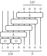
(a)

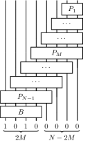
(b)

Figure 15: Realizations of the Bethe Ansatz with open boundary conditions. Fig. 15(a) depicts the tensor network of (A.8). Fig. 15(b) depicts the ABC to prepare (A.8) with unit norm.

Let us state the connection with the quantum circuit for free fermions with open boundaries of Subsection 4.1. We focus on the XXZ model with open boundary conditions at the free-fermion point $\Delta=0$. If we set $\Delta=0$ into (A.3) and (A.7), we obtain

$$B(q_{a},q_{b})=y_{a}+\frac{1}{y_{a}}+y_{b}+\frac{1}{y_{b}}\ ,\quad\alpha_{a}=1\ .$$ (A.13)

Since

$$B(p_{1},p_{2})=B(p_{2},p_{1})\ ,\quad B(p_{1},p_{2})=B(-p_{1},p_{2})=B(p_{1},-p_{2})=B(-p_{1},-p_{2})\ ,$$ (A.14)

we can strip scattering amplitudes out of (A.8) and write

$$|\Psi_{M}\rangle=\left[\underset{1\leq b<a\leq M}{\prod}B(p_{a},p_{b})\right]\sum_{\epsilon_{c}=\pm 1}\left[\,\prod_{d=1}^{M}\epsilon_{d}\right]|\Phi(\epsilon_{1}p_{1},\ldots,\epsilon_{M}p_{M})\rangle\ .$$ (A.15)

Therefore, we can remove the scattering amplitudes as an overall normalization of Bethe states with open boundary conditions. The result of the removal is (4.7).  Moreover, $\ket{\psi_{\mathrm{in}}}$ reduces to (4.8) at $\Delta=0$ and the unitaries $P_{k}$ and $B$ decompose as stated in Fig. 16(a)–16(b) and 4(b), respectively.

(a)

(b)

Figure 16: Factorization of $P_{k}$ into two-qubit unitaries and single-qubit rotations at the free-fermion point. Fig. 16(a) depicts the factorization of short unitaries $(1\leq k<2M)$. Fig. 16(b) depicts the factorization of long unitaries $(2M\leq k<N)$.

Appendix B Algebraic Bethe Circuits for Free Fermions

The unitaries $P_{k}$ of ABC for free fermions with open boundaries of Subsection 4.1 are layers of two-qubit unitaries, matchgates in particular [14, 77], and a single-qubit rotation for the small unitaries. Fig. 16(a)–16(b) shows the factorization of unitaries into matchgates. In this appendix, we provide closed formulae one- and two-qubit gates that did not appear in [14]. We also provide a new proof of their unitarity that does not rely on the connection with ABC.

Matchgates are based on the Bethe states of one magnon with one quasi-momentum $q_{a}$ in $q_{1},\ldots,q_{2M}$ over $k$ qubits, where the quasi-momenta are (A.1). These Bethe states read

$$|\Psi_{k,a}\rangle:=\overset{k}{\underset{n=1}{\sum}}\,y_{a}^{n-1}\,\sigma_{n}^{-}\ket{0}^{\otimes k}$$ (B.1)

where $y_{a}$ are (A.2). If $1\leq k<2M$, there are $k$ linearly independent Bethe states. We choose them to be the Bethe states of quasi-momenta $q_{1},\ldots,q_{k}$. If $2M\leq k<{N}$, there are $M$ linearly independent Bethe states, associated to the quasi-momenta $q_{1},\ldots,q_{2M}$. The Gram matrix of the Bethe states over $k$ qubits thus chosen is positive definite and Hermitian. Let

$$L_{k}:=\min(k,2M)\ .$$ (B.2)

The Gram matrix of the Bethe states reads

$$C_{k}=\begin{bmatrix}C_{11}&C_{12}&\ldots&C_{1L_{k}}\\ C_{21}&C_{22}&\ldots&C_{2L_{k}}\\ \ldots&\ldots&\ldots&\ldots\\ C_{L_{k}1}&C_{L_{k}2}&\ldots&C_{L_{k}L_{k}}\\ \end{bmatrix}\ ,$$ (B.3)

where the entries are

$$C_{k,ab}:=\langle\Psi_{k,a}|\Psi_{k,b}\rangle\ .$$ (B.4)

The matchgates of the quantum circuit are two-qubit unitaries based on the Gram matrix:

$$F_{k,a}=\begin{bmatrix}&1&0&0&0\\ &0&{u}^{*}_{k,a}&v_{k,a}&0\\ &0&-{v}^{*}_{k,a}&u_{k,a}&0\\ &0&0&0&1\\ \end{bmatrix}\quad 1\leq a<L_{k}\ .$$ (B.5)

The entries are

$$\begin{split}u_{k,a}=\frac{(-1)^{a-1}}{y_{1}^{*}\ldots y_{a-1}^{*}}\frac{{\det}_{a}C_{k+1,a\rightarrow e}}{\sqrt{{\det}_{a-1}C_{k}{\det}_{a}C_{k+1}}}\ ,\quad v_{k,a}=y_{a}\sqrt{\frac{{\det}_{a}C_{k}{\det}_{a-1}C_{k+1}}{{\det}_{a-1}C_{k}{\det}_{a}C_{k+1}}}\ ,\\ \end{split}$$ (B.6)

where $\det_{a}C_{k}$ denotes the upper-left minor of order $a$ of $C_{k}$ and ${C}_{k,a\rightarrow e}$ denotes the matrix that results from the replacement of the $a$-th row of ${C}_{k}$ by

$$e=\begin{bmatrix}1&1&\dots&1\end{bmatrix}.$$ (B.7)

The quantum circuit also comprises the single-qubit rotation

$$U_{k}=\begin{bmatrix}1&0\\ 0&\exp(\operatorname{i\!}\phi_{k})\end{bmatrix}\ ,$$ (B.8)

where

$$\exp(\operatorname{i\!}\phi_{k})=\prod_{a=1}^{k}\sqrt{\frac{y_{k+1}-y_{a}}{{y}^{*}_{k+1}-{y}^{*}_{a}}}\ .$$ (B.9)

Single-qubit rotations are straightforwardly unitary. It remains to demonstrate the matchgates (B.5) are unitary as well.

Unitarity is equivalent to

$$|{\det}_{a}\!\operatorname{\mathit{C}}_{k+1,a\to e}\!|^{2}\!-|y_{1}\dots y_{a-1}|^{2}{\det}_{a-1}\operatorname{\mathit{C}}_{k}{\det}_{a}\operatorname{\mathit{C}}_{k+1}+|y_{1}\dots y_{a}|^{2}{\det}_{a}\operatorname{\mathit{C}}_{k}{\det}_{a-1}\operatorname{\mathit{C}}_{k+1}=0\ .$$ (B.10)

The first step we take is the use of the recursion relation

$$C_{k+1,ab}={y}^{*}_{a}y_{b}C_{k,ab}+1\ ,\quad C_{0,ab}=1\ ,$$ (B.11)

to write

$$|y_{1}\dots y_{a}|^{2}{\det}_{a}\operatorname{\mathit{C}}_{k}={\det}_{a}(\operatorname{\mathit{C}}_{k+1}-E)\ ,$$ (B.12)

where

$$E=\begin{bmatrix}1&1&\ldots&1\\ 1&1&\ldots&1\\ \ldots&\ldots&\ldots&\ldots\\ 1&1&\ldots&1\end{bmatrix}\ .$$ (B.13)

Since the subscript $k+1$ is fixed until the end of the proof, we define

$$\operatorname{\mathit{C}}:=\operatorname{\mathit{C}}_{k+1}\ .$$ (B.14)

We use the identity of block-diagonal matrices

$$\det\begin{bmatrix}P&Q\\ R&S\end{bmatrix}=\det S{\det}(P-RS^{-1}Q)\quad\mathrm{if}\quad\!\!\!\det S\neq 0\ ,$$ (B.15)

to write

$$\begin{split}&\frac{{\det}_{a}\operatorname{\mathit{C}}_{a\to e}}{\det_{a-1}\operatorname{\mathit{C}}}=1-e^{t}C_{a-1}^{-1}c_{a}\ ,\\ &\frac{{\det}_{a}\operatorname{\mathit{C}}}{\det_{a-1}\operatorname{\mathit{C}}}=C_{aa}-c_{a}^{\dagger}C_{a-1}^{-1}c_{a}\ ,\\ &\frac{{\det}_{a}(\operatorname{\mathit{C}}-E)}{\det_{a-1}(\operatorname{\mathit{C}}-E)}=C_{aa}-1-(c_{a}-e)^{\dagger}(C_{a-1}-E)^{-1}(c_{a}-e)\ ,\end{split}$$ (B.16)

where

$$c_{a}=\begin{bmatrix}C_{a1}\\ C_{a2}\\ \ldots\\ C_{aa-1}\end{bmatrix}\ ,\quad C_{a}-1=\begin{bmatrix}C_{11}&C_{12}&\ldots&C_{1a-1}\\ C_{21}&C_{22}&\ldots&C_{2a-1}\\ \ldots&\ldots&\ldots&\ldots\\ C_{a-11}&C_{a-12}&\ldots&C_{a-1a-1}\end{bmatrix}\ .$$ (B.17)

If we introduce (B.16) into (B.10), we obtain

$$\begin{split}{\det}_{a-1}\operatorname{\mathit{C}}\,[(e^{t}C_{a-1}^{-1}c_{a})(c_{a}^{\dagger}C_{a-1}^{-1}e)-e^{t}C_{a-1}^{-1}c_{a}-c_{a}^{\dagger}C_{a-1}^{-1}e]+{\det}_{a-1}(\operatorname{\mathit{C}}-E)[c_{a}^{\dagger}C_{a-1}^{-1}c_{a}\\ -c_{a}^{\dagger}(C_{a-1}-E)^{-1}c_{a}+e^{t}(C_{a-1}-E)^{-1}c_{a}+c_{a}^{\dagger}(C_{a-1}-E)^{-1}c_{a}]=0\ ,\end{split}$$ (B.18)

where we have used that the identity (B.15) implies

$${\det}_{a-1}(\operatorname{\mathit{C}}-E)[1+e^{t}(C_{a-1}-E)^{-1}e]={\det}_{a-1}\operatorname{\mathit{C}}\ .$$ (B.19)

Let us consider now the identity

$$(C_{a-1}-E)^{-1}-E^{-1}=\big{(}C_{a-1}^{-1}e\big{)}\big{[}e^{t}(C_{a-1}-E)^{-1}\big{]},$$ (B.20)

where we have used the factorization $E=e\otimes e^{t}$. The positive definiteness of $C_{a-1}$ enables us to write

$$1-e^{t}C_{a-1}e=\det\left[C_{a-1}^{-1/2}(C_{a-1}-E)C_{a-1}^{-1/2}\right]=\frac{\det_{a-1}(C-E)}{\det_{a-1}C}\ .$$ (B.21)

The introduction of this identity into (B.20) provides

$$\frac{\det_{a-1}(C-E)}{\det_{a-1}C}e^{t}(C_{a-1}-E)^{-1}=e^{t}C_{a-1}^{-1}\ .$$ (B.22)

The positive definiteness of $C_{a-1}-E$ holds due to the recursion relation (B.11) and enables us to write

$$1+e^{t}(C_{a-1}-E)^{-1}e=\det\left[(C_{a-1}-E)^{-1/2}C_{a-1}(C_{a-1}-E)^{-1/2}\right]=\frac{\det_{a-1}C}{\det_{a-1}(C-E)}\ .$$ (B.23)

The introduction of this identity into (B.20) provides

$$\frac{\det_{a-1}C}{\det_{a-1}(C-E)}C_{a-1}^{-1}e=(C_{a-1}-E)^{-1}e\ .$$ (B.24)

The use of (B.22) and (B.24) in (B.18), makes the left-hand side vanish identically. The unitarity of matchgates is thus proven.

Appendix C Details on the $N=5$ and $N=6$ circuits

The circuits in Fig. 13 build folded XXZ eigenstates with one magnon and two domain walls in chains with $N=5$ and $N=6$ bulk sites. They exhibit some simplifications with respect to the general scheme explained in Subsection 4.3. In order to clarify their validity, we detail here how the state of the physical register evolves through the different modules when a magnon is present at the position $n$ of $R_{\mathrm{aux}}$. The register $R_{\mathrm{phys}}$ starts in one of the domain reference states listed in (5.1). The position of the $|01\rangle$ domain wall is then updated by the presence of the magnon at $R_{\mathrm{aux},n}$ following the rules in (3.31) and (3.32). The position of the $|10\rangle$ domain wall is updated next. These operations correspond respectively to the red- and green-shadowed areas of the circuits in Fig. 13. The blue-shadowed areas describe the insertion of the magnon into the appropriate location of $R_{\mathrm{phys}}$ using the information in $R_{\mathrm{c}}$, while the yellow areas reset $R_{\mathrm{c}}$. For convenience, we include below both the state of $R_{\mathrm{phys}}$ and $R_{\mathrm{c}}$ at each stage.

Intermediate states along the $N=5$ circuit

$$\begin{array}[]{ccccccccc}\text{Position of the}&|\Psi_{0,D}\rangle&&|01\rangle\mathrm{\;DW\;module}&&|10\rangle\mathrm{\;DW\;module}&&\!\!\!\!\!\!\mathrm{Magnon\;insertion}\!\!\!\!\!\!&\\ \text{magnon in}\leavevmode\nobreak\ R_{\mathrm{aux}}&&&&&&&&\\ &|00110\rangle\otimes|00\rangle&\longrightarrow&|11110\rangle\otimes|10\rangle&\longrightarrow&|11000\rangle\otimes|11\rangle&\longrightarrow&|11001\rangle\otimes|11\rangle\\ n=3&|00111\rangle\otimes|00\rangle&\longrightarrow&|11111\rangle\otimes|10\rangle&\longrightarrow&|11111\rangle\otimes|10\rangle&\longrightarrow&|11101\rangle\otimes|10\rangle\\ &|00011\rangle\otimes|00\rangle&\longrightarrow&|01111\rangle\otimes|10\rangle&\longrightarrow&|01111\rangle\otimes|10\rangle&\longrightarrow&|01101\rangle\otimes|10\rangle\\ &&&&&&&&\\ &|00110\rangle\otimes|00\rangle&\longrightarrow&|11110\rangle\otimes|10\rangle&\longrightarrow&|11110\rangle\otimes|10\rangle&\longrightarrow&|11010\rangle\otimes|10\rangle\\ n=2&|00111\rangle\otimes|00\rangle&\longrightarrow&|11111\rangle\otimes|10\rangle&\longrightarrow&|11111\rangle\otimes|10\rangle&\longrightarrow&|11011\rangle\otimes|10\rangle\\ &|00011\rangle\otimes|00\rangle&\longrightarrow&|00011\rangle\otimes|00\rangle&\longrightarrow&|00011\rangle\otimes|00\rangle&\longrightarrow&|01011\rangle\otimes|00\rangle\\ &&&&&&&&\\ &|00110\rangle\otimes|00\rangle&\longrightarrow&00110\rangle\otimes|00\rangle&\longrightarrow&00110\rangle\otimes|00\rangle&\longrightarrow&|10110\rangle\otimes|00\rangle\\ n=1&|00111\rangle\otimes|00\rangle&\longrightarrow&00111\rangle\otimes|00\rangle&\longrightarrow&|10111\rangle\otimes|00\rangle&\longrightarrow&|10111\rangle\otimes|00\rangle\\ &|00110\rangle\otimes|00\rangle&\longrightarrow&00011\rangle\otimes|00\rangle&\longrightarrow&00011\rangle\otimes|00\rangle&\longrightarrow&|10011\rangle\otimes|00\rangle\\ \end{array}$$

Intermediate states along the $N=6$ circuit

$$\begin{array}[]{ccccccccc}\text{Position of the}&|\Psi_{0,D}\rangle&&|01\rangle\mathrm{\;DW\;module}&&|10\rangle\mathrm{\;DW\;module}&&\!\!\!\!\!\!\mathrm{Magnon\;insertion}\!\!\!\!\!\!&\\ \text{magnon in}\leavevmode\nobreak\ R_{\mathrm{aux}}&&&&&&&&\\ &|001100\rangle\otimes|00\rangle&\longrightarrow&|111100\rangle\otimes|10\rangle&\longrightarrow&|110000\rangle\otimes|11\rangle&\longrightarrow&|110001\rangle\otimes|11\rangle\\ &|001110\rangle\otimes|00\rangle&\longrightarrow&|111110\rangle\otimes|10\rangle&\longrightarrow&|111000\rangle\otimes|11\rangle&\longrightarrow&|111001\rangle\otimes|11\rangle\\ n=4&|001111\rangle\otimes|00\rangle&\longrightarrow&|111111\rangle\otimes|10\rangle&\longrightarrow&|111111\rangle\otimes|10\rangle&\longrightarrow&|111101\rangle\otimes|10\rangle\\ &|000110\rangle\otimes|00\rangle&\longrightarrow&011110\rangle\otimes|10\rangle&\longrightarrow&011000\rangle\otimes|11\rangle&\longrightarrow&011001\rangle\otimes|11\rangle\\ &|000111\rangle\otimes|00\rangle&\longrightarrow&|011111\rangle\otimes|10\rangle&\longrightarrow&|011111\rangle\otimes|10\rangle&\longrightarrow&|011101\rangle\otimes|10\rangle\\ &|000011\rangle\otimes|00\rangle&\longrightarrow&|001111\rangle\otimes|00\rangle&\longrightarrow&|001111\rangle\otimes|10\rangle&\longrightarrow&|001101\rangle\otimes|10\rangle\\ &&&&&&&&\\ &|001100\rangle\otimes|00\rangle&\longrightarrow&|111100\rangle\otimes|10\rangle&\longrightarrow&|110000\rangle\otimes|11\rangle&\longrightarrow&|110010\rangle\otimes|11\rangle\\ &|001110\rangle\otimes|00\rangle&\longrightarrow&|111110\rangle\otimes|10\rangle&\longrightarrow&|111110\rangle\otimes|11\rangle&\longrightarrow&|111010\rangle\otimes|11\rangle\\ n=3&|001111\rangle\otimes|00\rangle&\longrightarrow&|111111\rangle\otimes|10\rangle&\longrightarrow&|111111\rangle\otimes|10\rangle&\longrightarrow&|111011\rangle\otimes|10\rangle\\ &|000110\rangle\otimes|00\rangle&\longrightarrow&|011110\rangle\otimes|10\rangle&\longrightarrow&|011110\rangle\otimes|11\rangle&\longrightarrow&|011010\rangle\otimes|11)\\ &|000111\rangle\otimes|00\rangle&\longrightarrow&|011111\rangle\otimes|10\rangle&\longrightarrow&|011111\rangle\otimes|10\rangle&\longrightarrow&|011011\rangle\otimes|10\rangle\\ &|000011\rangle\otimes|00\rangle&\longrightarrow&|000011\rangle\otimes|00\rangle&\longrightarrow&|000011\rangle\otimes|10\rangle&\longrightarrow&|001101\rangle\otimes|10\rangle\\ &&&&&&&\\ &|001100\rangle\otimes|00\rangle&\longrightarrow&|111100\rangle\otimes|10\rangle&\longrightarrow&|111100\rangle\otimes|10\rangle&\longrightarrow&|110100\rangle\otimes|10\rangle\\ &|001110\rangle\otimes|00\rangle&\longrightarrow&|111110\rangle\otimes|10\rangle&\longrightarrow&|111110\rangle\otimes|10\rangle&\longrightarrow&|110110\rangle\otimes|10\rangle\\ n=2&|001111\rangle\otimes|00\rangle&\longrightarrow&|111111\rangle\otimes|10\rangle&\longrightarrow&|111111\rangle\otimes|10\rangle&\longrightarrow&|110111\rangle\otimes|10\rangle\\ &|000110\rangle\otimes|00\rangle&\longrightarrow&|000110\rangle\otimes|00\rangle&\longrightarrow&|000110\rangle\otimes|00\rangle&\longrightarrow&|010110\rangle\otimes|00\rangle\\ &|000111\rangle\otimes|00\rangle&\longrightarrow&|000111\rangle\otimes|00\rangle&\longrightarrow&|000111\rangle\otimes|00\rangle&\longrightarrow&|010111\rangle\otimes|00\rangle\\ &|000011\rangle\otimes|00\rangle&\longrightarrow&|000011\rangle\otimes|00\rangle&\longrightarrow&|000011\rangle\otimes|00\rangle&\longrightarrow&|010011\rangle\otimes|00\rangle\\ &&&&&&&&\\ &|001100\rangle\otimes|00\rangle&\longrightarrow&|001100\rangle\otimes|00\rangle&\longrightarrow&|001100\rangle\otimes|00\rangle&\longrightarrow&|101100\rangle\otimes|00\rangle\\ &|001110\rangle\otimes|00\rangle&\longrightarrow&|001110\rangle\otimes|00\rangle&\longrightarrow&|001110\rangle\otimes|00\rangle&\longrightarrow&|101110\rangle\otimes|00\rangle\\ n=1&|001111\rangle\otimes|00\rangle&\longrightarrow&|001111\rangle\otimes|00\rangle&\longrightarrow&|001111\rangle\otimes|00\rangle&\longrightarrow&|101111\rangle\otimes|00\rangle\\ &|000110\rangle\otimes|00\rangle&\longrightarrow&|000110\rangle\otimes|00\rangle&\longrightarrow&|000110\rangle\otimes|00\rangle&\longrightarrow&|100110\rangle\otimes|00\rangle\\ &|000111\rangle\otimes|00\rangle&\longrightarrow&|000111\rangle\otimes|00\rangle&\longrightarrow&|000111\rangle\otimes|00\rangle&\longrightarrow&|100111\rangle\otimes|00\rangle\\ &|000011\rangle\otimes|00\rangle&\longrightarrow&|000011\rangle\otimes|00\rangle&\longrightarrow&900011\rangle\otimes|00\rangle&\longrightarrow&|100011\rangle\otimes|00\rangle\\ \end{array}$$

Appendix D Error Mitigation Details

The implementation of CDR is very similar to that in [78]. For the training circuits we replace all but 50 non-Clifford gates, selecting them randomly and replacing them probabilistically with a Clifford gate as detailed in [78]. The exact and noisy expectation values obtained from the training set of near Clifford circuits are used to learn a linear model, which is then applied to the noisy expectation value of the original circuit. We learn a single model to mitigate the energy instead of a different model for each Pauli term. A similar reasoning applies to the charges $\langle Q_{1}\rangle$ and $\langle Q_{2}\rangle$, although in this case, we must take into account the constants $N/2$ and $(N+1)/2$ for each charge, respectively. We mitigate these observables without these constants and add them afterward. An example applying CDR to mitigate the energy with all-to-all and nearest-neighbor connectivity is shown in Fig. 17. The slope of the lines with nearest-neighbor connectivity are greater, indicating a stronger effective depolarizing noise. Figs. 18 and 19 show similar results for $\langle Q_{1}\rangle$ and $\langle Q_{2}\rangle$, respectively

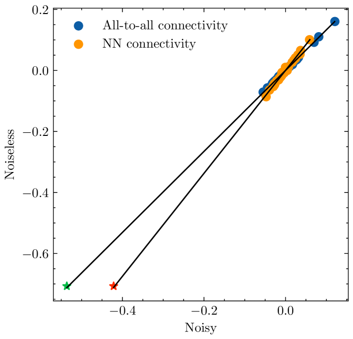
(a)

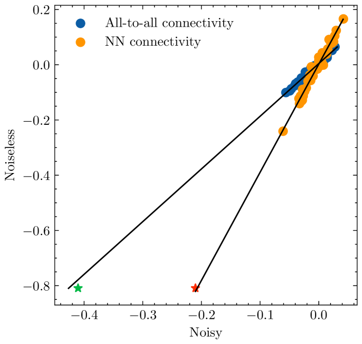
(b)

Figure 17: Distribution of exact and noisy energies produced by the near-Clifford training circuits with all-to-all and nearest-neighbor (NN) connectivity. Fig. 17(a) corresponds to the $N=5$ state, while Fig. 17(b) corresponds to the $N=6$ state. The green and red stars show the noisy and exact result for the energy for each connectivity.

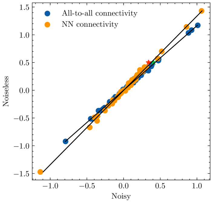
(a)

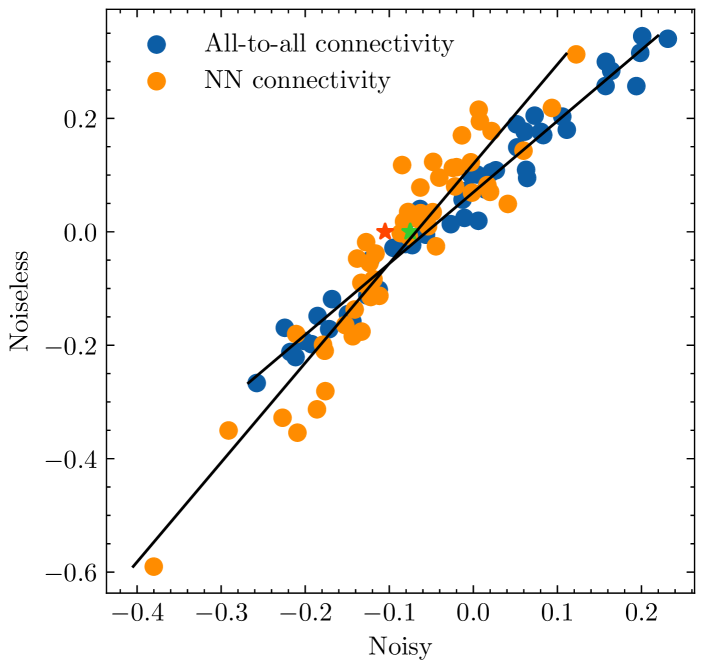
(b)

Figure 18: Distribution of exact and noisy $\langle Q_{1}\rangle-N/2$ produced by the near-Clifford training circuits with all-to-all and nearest-neighbor (NN) connectivity. Fig. 18(a) corresponds to the $N=5$ state, while Fig. 18(b) corresponds to the $N=6$ state. The green and red stars show the noisy and exact result for the energy for each connectivity.

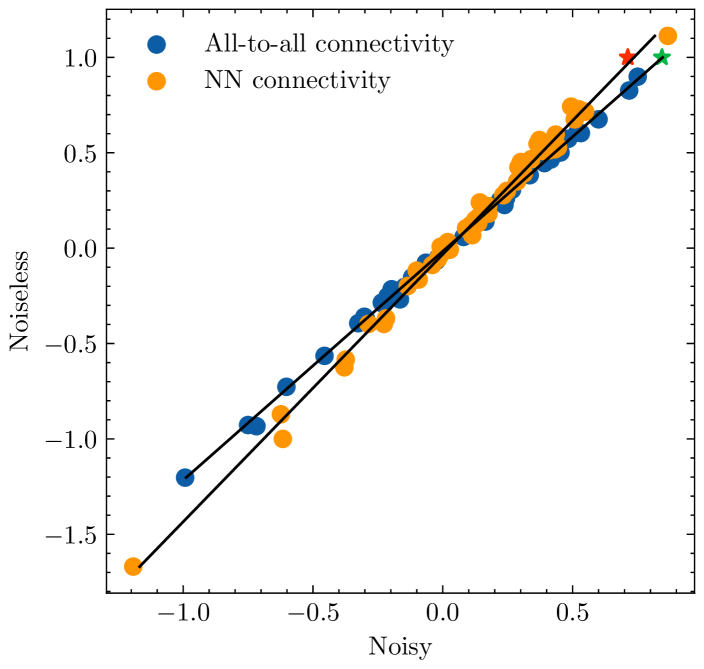
(a)

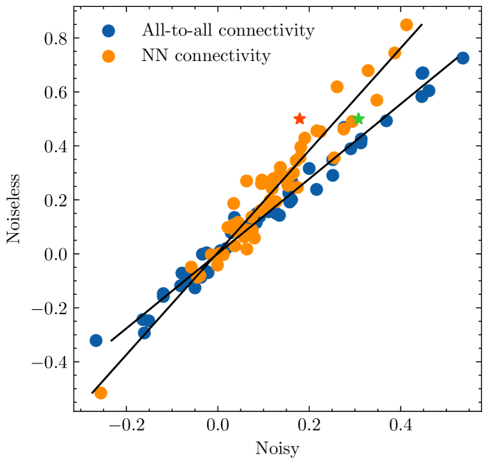
(b)

Figure 19: Distribution of exact and noisy $\langle Q_{2}\rangle-(N+1)/2$ produced by the near-Clifford training circuits with all-to-all and nearest-neighbor (NN) connectivity. Fig. 19(a) corresponds to the $N=5$ state, while Fig. 19(b) corresponds to the $N=6$ state. The green and red stars show the noisy and exact result for the energy for each connectivity.

References

- [1] F. Verstraete, J.I. Cirac, J.I. Latorre, “Quantum circuits for strongly correlated quantum systems”, J. Phys. A 79 (2009) [0804.1888].
- [2] Z. Jiang, K.J. Sung, K. Kechedzhi, V.N. Smelyanskiy, S. Boixo, “Quantum Algorithms to Simulate Many-Body Physics of Correlated Fermions”, Phys. Rev. Applied 9 (2018) 044036 [1711.05395].
- [3] I.D. Kivlichan, J. McClean, N. Wiebe, C. Gidney, A. Aspuru-Guzik, G.K.-L. Chan et al., “Quantum Simulation of Electronic Structure with Linear Depth and Connectivity”, Phys. Rev. Lett. 120 (2018) 110501.
- [4] A. Cervera-Lierta, “Exact Ising model simulation on a quantum computer”, Quantum 2 (2018) 114 [1807.07112].
- [5] M. Farreras, A. Cervera-Lierta, “Simulation of the 1d XY model on a quantum computer”, 2410.21143.
- [6] L.G. Valiant, “Quantum circuits that can be simulated classically in polynomial time”, SIAM J. Comput. 31 (2002) 1229.
- [7] B.M. Terhal, D.P. DiVincenzo, “Classical simulation of noninteracting-fermion quantum circuits”, Phys. Rev. A 65 (2002) 032325.
- [8] R. Jozsa, A. Miyake, “Matchgates and classical simulation of quantum circuits”, Proc. R. Soc. A 464 (2008) 3089 [0804.4050].
- [9] B. Sutherland, Beautiful Models, World Scientific Publishing Company (2004).
- [10] V.E. Korepin, N.M. Bogoliubov, A.G. Izergin, Quantum Inverse Scattering Method and Correlation Functions, Cambridge Monographs on Mathematical Physics, Cambridge University Press (1993), 10.1017/CBO9780511628832.
- [11] L.D. Faddeev, “How Algebraic Bethe Ansatz works for integrable model”, arXiv e-prints (1996) [hep-th/9605187].
- [12] J.S. Van Dyke, G.S. Barron, N.J. Mayhall, E. Barnes, S.E. Economou, “Preparing Bethe Ansatz Eigenstates on a Quantum Computer”, PRX Quantum 2 (2021) 040329 [2103.13388].
- [13] A. Sopena, M.H. Gordon, D. García-Martín, G. Sierra, E. López, “Algebraic Bethe Circuits”, Quantum 6 (2022) 796 [2202.04673].
- [14] R. Ruiz, A. Sopena, M.H. Gordon, G. Sierra, E. López, “The Bethe Ansatz as a Quantum Circuit”, Quantum 8 (2024) 1356 [2309.14430].
- [15] D. Raveh, R.I. Nepomechie, “Deterministic Bethe state preparation”, Quantum 8 (2024) 1510 [2403.03283].
- [16] J.S. Van Dyke, E. Barnes, S.E. Economou, R.I. Nepomechie, “Preparing exact eigenstates of the open XXZ chain on a quantum computer”, J. Phys. A 55 (2022) 055301 [2109.05607].
- [17] W. Li, M. Okyay, R.I. Nepomechie, “Bethe states on a quantum computer: success probability and correlation functions”, J. Phys. A 55 (2022) 355305 [2201.03021].
- [18] C. Trippe, F. Göhmann, A. Klümper, “Thermodynamics and short-range correlations of the XXZ chain close to its triple point”, J. Stat. Mech. 2010 (2010) 01021 [0912.1739].
- [19] L. Zadnik, M. Fagotti, “The Folded Spin-1/2 XXZ Model: I. Diagonalisation, Jamming, and Ground State Properties”, SciPost Phys. Core 4 (2021) 010 [2009.04995].
- [20] L. Zadnik, K. Bidzhiev, M. Fagotti, “The Folded Spin-1/2 XXZ Model: II. Thermodynamics and Hydrodynamics with a Minimal Set of Charges”, SciPost Phys. 10 (2021) 099 [2011.01159].
- [21] B. Pozsgay, T. Gombor, A. Hutsalyuk, Y. Jiang, L. Pristyák, E. Vernier, “Integrable spin chain with Hilbert space fragmentation and solvable real-time dynamics”, Phys. Rev. E 104 (2021) 044106 [2105.02252].
- [22] G.I. Menon, M. Barma, D. Dhar, “Conservation laws and integrability of a one-dimensional model of diffusing dimers”, J. Stat. Phys. 86 (1997) 1237 [cond-mat/9703059].
- [23] Z.-C. Yang, F. Liu, A.V. Gorshkov, T. Iadecola, “Hilbert-Space Fragmentation from Strict Confinement”, Phys. Rev. Lett. 124 (2020) 207602 [1912.04300].
- [24] Z. Papić, “Weak ergodicity breaking through the lens of quantum entanglement”, in Entanglement in Spin Chains: From Theory to Quantum Technology Applications, A. Bayat, S. Bose, H. Johannesson, eds., (Cham), pp. 341–395, Springer International Publishing, 2022, DOI [2108.03460].
- [25] S. Moudgalya, B.A. Bernevig, N. Regnault, “Quantum many-body scars and hilbert space fragmentation: a review of exact results”, Rep. Prog. Phys. 85 (2022) 086501 [2109.00548].
- [26] K. Bidzhiev, M. Fagotti, L. Zadnik, “Macroscopic effects of localised measurements in jammed states of quantum spin chains”, Phys. Rev. Lett. 128 (2022) 130603 [2108.03230].
- [27] L. Zadnik, S. Bocini, K. Bidzhiev, M. Fagotti, “Measurement catastrophe and ballistic spread of charge density with vanishing current”, J. Phys. A 55 (2022) 474001 [2111.06325].
- [28] K. Kim, F. Yang, K. Mølmer, J. Ahn, “Realization of an Extremely Anisotropic Heisenberg Magnet in Rydberg Atom Arrays”, Phys. Rev. X 14 (2024) 011025 [2307.04342].
- [29] F. Yang, H. Yarloo, H.-C. Zhang, K. Mølmer, A.E.B. Nielsen, “Probing Hilbert Space Fragmentation with Strongly Interacting Rydberg Atoms”, arXiv e-prints (2024) [2403.13790].
- [30] B. Pozsgay, “A Yang-Baxter integrable cellular automaton with a four site update rule”, J. Phys. A 54 (2021) 384001 [2106.00696].
- [31] S. Gopalakrishnan, A. Morningstar, R. Vasseur, V. Khemani, “Distinct universality classes of diffusive transport from full counting statistics”, Phys. Rev. B 109 (2024) 024417 [2203.09526].
- [32] T. Gombor, B. Pozsgay, “Integrable spin chains and cellular automata with medium-range interaction”, Phys. Rev. E 104 (2021) 054123 [2108.02053].
- [33] F.C. Alcaraz, R.Z. Bariev, “An Exactly Solvable Constrained XXZ Chain”, (1999) [cond-mat/9904042].
- [34] F.C. Alcaraz, R.Z. Bariev, “Integrable models of strongly correlated particles with correlated hopping”, Phys. Rev. B 59 (1999) 3373 [cond-mat/9904129].
- [35] I.N. Karnaukhov, A.A. Ovchinnikov, “One-dimensional strongly interacting Luttinger liquid of lattice spinless fermions”, Europhys. Lett. 57 (2002) 540 [cond-mat/0110289].
- [36] F.C. Alcaraz, M.J. Lazo, “Exactly solvable interacting vertex models”, J. Stat. Mech. 2007 (2007) 08008 [0706.2178].
- [37] N. Abarenkova, A. Pronko, “Temperature Correlation Function in the Absolutely Anisotropic XXZ Heisenberg Magnet”, Theor. Math. Phys. 131 (2002) 690.
- [38] N.M. Bogoliubov, C. Malyshev, “The correlation functions of the XXZ Heisenberg chain in the case of zero or infinite anisotropy, and random walks of vicious walkers”, St. Petersburg Mathematical Journal 22 (2011) 359 [0912.1138].
- [39] N.M. Bogoliubov, C.L. Malyshev, “Ising limit of a Heisenberg XXZ magnet and some temperature correlation functions”, Theor. Math. Phys. 169 (2011) 1517 [1106.5455].
- [40] N.M. Bogolyubov, C.L. Malyshev, “Integrable models and combinatorics”, Russ. Math. Surv. 70 (2015) 789.
- [41] M. Ganahl, M. Haque, H.G. Evertz, “Quantum Bowling: Particle-hole transmutation in one-dimensional strongly interacting lattice models”, arXiv e-prints (2013) [1302.2667].
- [42] B. Pozsgay, T. Gombor, A. Hutsalyuk, “Integrable hard rod deformation of the Heisenberg spin chains”, Phys. Rev. E 104 (2021) [2108.13724].
- [43] M. Borsi, L. Pristyák, B. Pozsgay, “Matrix product symmetries and breakdown of thermalization from hard rod deformations”, Phys. Rev. Lett. 131 (2023) [2302.07219].
- [44] M. Fagotti, “Quantum Jamming Brings Quantum Mechanics to Macroscopic Scales”, Phys. Rev. X 14 (2024) 021015 [2307.14979].
- [45] S.K. Singh, A. Dhar, H. Spohn, A. Kundu, “Thermalization and hydrodynamics in an interacting integrable system: the case of hard rods”, 2310.18684.
- [46] F.C. Alcaraz, M.J. Lazo, “The Bethe ansatz as a matrix product ansatz”, J. Phys. A 37 (2004) L1 [cond-mat/0304170].
- [47] F.C. Alcaraz, M.J. Lazo, “Exact solutions of exactly integrable quantum chains by a matrix product ansatz”, J. Phys. A 37 (2004) 4149 [cond-mat/0312373].
- [48] F.C. Alcaraz, M.J. Lazo, “Generalization of the matrix product ansatz for integrable chains”, J. Phys. A 39 (2006) 11335 [cond-mat/0608177].
- [49] H. Katsura, I. Maruyama, “Derivation of the matrix product ansatz for the Heisenberg chain from the algebraic Bethe ansatz”, J. Phys. A 43 (2010) 175003 [0911.4215].
- [50] V. Murg, V.E. Korepin, F. Verstraete, “Algebraic Bethe ansatz and tensor networks”, Phys. Rev. B 86 (2012) [1201.5627].
- [51] J.I. Cirac, D. Pérez-García, N. Schuch, F. Verstraete, “Matrix product states and projected entangled pair states: Concepts, symmetries, theorems”, Rev. Mod. Phys. 93 (2021) 045003 [2011.12127].
- [52] A. Sopena, R. Ruiz, “XXZ_folded 2.0”, Zenodo (2024) .
- [53] J. Preskill, “Quantum Computing in the NISQ era and beyond”, Quantum 2 (2018) 79 [1801.00862].
- [54] S. Efthymiou, S. Ramos-Calderer, C. Bravo-Prieto, A. Pérez-Salinas, D. García-Martín, A. Garcia-Saez et al., “Qibo: a framework for quantum simulation with hardware acceleration”, Quantum Sci. Technol. 7 (2022) 015018 [2009.01845].
- [55] C.R. Clark, H.N. Tinkey, B.C. Sawyer, A.M. Meier, K.A. Burkhardt, C.M. Seck et al., “High-Fidelity Bell-State Preparation with Ca + 40 Optical Qubits”, Phys. Rev. Lett. 127 (2021) 130505 [2105.05828].
- [56] L. Ding, M. Hays, Y. Sung, B. Kannan, J. An, A. Di Paolo et al., “High-Fidelity, Frequency-Flexible Two-Qubit Fluxonium Gates with a Transmon Coupler”, Phys. Rev. X 13 (2023) 031035 [2304.06087].
- [57] S.J. Evered, D. Bluvstein, M. Kalinowski, S. Ebadi, T. Manovitz, H. Zhou et al., “High-fidelity parallel entangling gates on a neutral-atom quantum computer”, Nature 622 (2023) 268 [2304.05420].
- [58] H. Zhang, C. Ding, D. Weiss, Z. Huang, Y. Ma, C. Guinn et al., “Tunable Inductive Coupler for High-Fidelity Gates Between Fluxonium Qubits”, PRX Quantum 5 (2024) 020326 [2309.05720].
- [59] J.J. Wallman, J. Emerson, “Noise tailoring for scalable quantum computation via randomized compiling”, Phys. Rev. A 94 (2016) 052325 [1512.01098].
- [60] A. Hashim, R.K. Naik, A. Morvan, J.-L. Ville, B. Mitchell, J.M. Kreikebaum et al., “Randomized Compiling for Scalable Quantum Computing on a Noisy Superconducting Quantum Processor”, Phys. Rev. X 11 (2021) 041039 [2010.00215].
- [61] E. Magesan, J.M. Gambetta, J. Emerson, “Scalable and Robust Randomized Benchmarking of Quantum Processes”, Phys. Rev. Lett. 106 (2011) 180504 [1009.3639].
- [62] H.-L. Huang, D. Wu, D. Fan, X. Zhu, “Superconducting quantum computing: a review”, Sci. China Inf. Sci. 63 (2020) 180501 [2006.10433].
- [63] D. Kielpinski, C. Monroe, D.J. Wineland, “Architecture for a large-scale ion-trap quantum computer”, Nature 417 (2002) 709.
- [64] J.P. Home, D. Hanneke, J.D. Jost, J.M. Amini, D. Leibfried, D.J. Wineland, “Complete Methods Set for Scalable Ion Trap Quantum Information Processing”, Science 325 (2009) 1227 [0907.1865].
- [65] V. Kaushal, B. Lekitsch, A. Stahl, J. Hilder, D. Pijn, C. Schmiegelow et al., “Shuttling-based trapped-ion quantum information processing”, AVS Quantum Sci. 2 (2020) 014101 [1912.04712].
- [66] F. Arute, K. Arya, R. Babbush, D. Bacon, J.C. Bardin, R. Barends et al., “Quantum supremacy using a programmable superconducting processor”, Nature 574 (2019) 505.
- [67] G. Li, Y. Ding, Y. Xie, “Tackling the Qubit Mapping Problem for NISQ-Era Quantum Devices”, in Proceedings of the Twenty-Fourth International Conference on Architectural Support for Programming Languages and Operating Systems, (Providence RI USA), pp. 1001–1014, ACM, Apr., 2019, DOI [1809.02573].
- [68] H. Pashayan, O. Reardon-Smith, K. Korzekwa, S.D. Bartlett, “Fast Estimation of Outcome Probabilities for Quantum Circuits”, PRX Quantum 3 (2022) 020361 [2101.12223].
- [69] P. Czarnik, A. Arrasmith, P.J. Coles, L. Cincio, “Error mitigation with Clifford quantum-circuit data”, Quantum 5 (2021) 592 [2005.10189].
- [70] F. Alcaraz, R. Bariev, “An exactly solvable constrained XXZ chain”, in Statistical Physics on the Eve of the 21st Century, M. Batchelor, L. Wille, eds., World Scientific, 1999 [cond-mat/9904042].
- [71] F.C. Alcaraz, M.J. Lazo, “Exactly solvable interacting vertex models”, J. Stat. Mech. 2007 (2007) P08008 [0706.2178].
- [72] P. Fendley, “Free fermions in disguise”, J. Phys. A 52 (2019) 335002 [1901.08078].
- [73] A. Chapman, S.J. Elman, R.L. Mann, “A Unified Graph-Theoretic Framework for Free-Fermion Solvability”, 2305.15625.
- [74] P. Fendley, B. Pozsgay, “Free fermions beyond Jordan and Wigner”, SciPost Phys. 16 (2024) 102 [2310.19897].
- [75] B. Pozsgay, “Quantum circuits with free fermions in disguise”, 2402.02984.
- [76] I. Vona, M. Mestyán, B. Pozsgay, “Exact real time dynamics with free fermions in disguise”, 2405.20832.
- [77] A. Sopena, R. Ruiz, “The-bethe-ansatz-as-a-quantum-circuit 1.0”, Zenodo (2024) .
- [78] A. Sopena, M.H. Gordon, G. Sierra, E. López, “Simulating quench dynamics on a digital quantum computer with data-driven error mitigation”, Quantum Sci. Technol. 6 (2021) 045003 [2103.12680].