Untangling Magellanic Streams

Abstract

The Magellanic Stream has long been known to contain multiple HI strands and corresponding stellar populations are beginning to be discovered. Combining an H3-selected sample with stars drawn from the Gaia catalog, we trace stars along a sub-dominant strand of the Magellanic Stream, as defined by gas content, across 30^∘ on the sky. We find that the dominant strand is devoid of stars with Galactocentric distance $\lesssim 55$ kpc while the subdominant strand shows a close correspondence to such stars. We conclude that (1) the two Stream strands have different origins, (2) they are likely only close in projection, (3) the subdominant strand is tidal in origin, and (4) the subdominant strand is composed of disk material, likely drawn from the disk of the Small Magellanic Cloud.

⁵NASA Hubble Fellow

1 Introduction

The Magellanic Clouds are the nearest example of a phenomenon that we understand to be common throughout the history of Universe — the infall of small galaxies onto large dark matter halos (Blumenthal et al., 1984; Davis et al., 1985). As such, they present our best opportunity to study this central aspect of galaxy evolution and refine how it is modeled (e.g., Cole et al., 2000). Is gravity or hydrodynamics primarily responsible for stripping gas out of such infalling galaxies (Mathewson et al., 1974; Lin & Lynden-Bell, 1977; Moore & Davis, 1994)? How do galaxy interactions, either between the Clouds themselves or with the Milky Way (hereafter the MW), affect the star formation rates within the small galaxies (Zaritsky & Harris, 2004; Harris & Zaritsky, 2009; Massana et al., 2022)? How can such infall events affect the larger galaxy onto which the small galaxies have fallen (Weinberg & Blitz, 2006; Fox et al., 2010; Garavito-Camargo et al., 2019; Lucchini et al., 2021; Carr et al., 2024)?

To address these and other questions, investigators have generated an increasingly sophisticated set of numerical simulations of the interaction (e.g., Lin & Lynden-Bell, 1977; Gardiner & Noguchi, 1996; Besla et al., 2010; Diaz & Bekki, 2012; Gómez et al., 2015; Pardy et al., 2018; Garavito-Camargo et al., 2019; Lucchini et al., 2021, 2024; Carr et al., 2024). This progress has led to a realization of the complexity of the system but also to a greater appreciation of its potential for leading us to a more complete understanding of such fundamental topics in astrophysics as the nature of the circumgalactic medium (Fox et al., 2010; Lucchini et al., 2021; Carr et al., 2024) and dark matter (Foote et al., 2023). To motivate, constrain, and exploit even more complex simulations, an ever increasing set of detailed observational constraints is needed.

Among the variety of interesting features of the Magellanic system that challenge models is the long gaseous tail that trails the Clouds, referred to as the Magellanic Stream (hereafter the MS; Dieter, 1971; Wannier & Wrixon, 1972; Mathewson et al., 1974). The MS is a set of apparently intertwined HI filaments (Cohen, 1982; Morras, 1983; Putman et al., 2003b; Nidever et al., 2008a) whose origin (LMC, Bridge, or SMC) is still debated (e.g., Nidever et al., 2008b; Fox et al., 2010; Diaz & Bekki, 2012; Pardy et al., 2018). The 3D geometry is unknown because of the difficulty in measuring distances to gas clouds (Putman et al., 2003b).

While arguments have often been framed around whether this gas was drawn out primarily by tidal forces (Fujimoto & Sofue, 1976; Lin & Lynden-Bell, 1977) or ram pressure (Meurer et al., 1985; Moore & Davis, 1994), the unavoidable nature of tides, the weak, fragmented nature of the leading arm (Putman et al., 1998), the ionized nature of the MS (Putman et al., 2003a), and the morphology of high velocity clouds (Putman et al., 2011) suggest that both physical phenomena will be part of a full understanding. Potential internal factors, such as winds that push gas outward and make it more susceptible to either tides or ram pressure, add yet another layer of complexity (Olano, 2004; Nidever et al., 2008b).

The tidal hypothesis for the origin of the MS offers hope for the presence of stars along the MS, which would then provide distance constraints, a better understanding of the geometry and, perhaps, of its origin. In contrast, the confirmed absence of stars in the MS would likewise be an important constraint and would favor a hydrodynamic origin scenario, such as the blowout plus stripping model of Nidever et al. (2008b). Searches for stars along the MS have generally yielded negative results (Recillas-Cruz, 1982; Brueck & Hawkins, 1983; Guhathakurta & Reitzel, 1998). More recently, tidal stellar features have been uncovered closer to the LMC-SMC system (Belokurov & Koposov, 2016; Mackey et al., 2016; Belokurov & Erkal, 2019; Deason et al., 2019) but a population tracing the MS has been elusive.

The H3 survey (Conroy et al., 2019) and follow-up observations have contributed to the body of work on the stellar counterpart of the MS in two studies. Zaritsky et al. (2020b), hereafter Z20, identified 15 stars that form a dynamically cold group that closely follows part of the MS in projection and matches roughly in radial velocity, but lacks the large negative angular momentum of the Clouds. Chandra et al. (2023), hereafter C23, identified 13 stars at greater Galactocentric distance, $60-120$ kpc, among a population of distant stars selected to match the large negative angular momentum of the Clouds about the MW’s x-axis. These, rather than the Z20 stars, appear to be more naturally identified as the stellar counterpart of the MS because of the angular momentum match and the closer agreement in distance with the simulations of Besla et al. (2012).

If the Z20 stars are not part of the MS, then what are they and what does the close association between these stars and at least some of the gas in the MS imply. The Z20 detection involved only 15 stars, making it difficult to trace the feature in detail and establish an unambiguous association with any specific component of the MS. Here we expand the sample by using the Z20 stars to aid us in selecting a Gaia DR3 sample of stars with which to better trace this population. In §2 we describe how we select stars from the Gaia catalog. In §3 we describe the distribution of those stars and our inferences regarding the nature of the MS.

2 Data

Our strategy is to use the H3 catalog to identify a pure sample of putative stellar stream stars, as identified by Z20, and then use those stars to train our selection of additional possible members of this population in the Gaia catalog. We will then examine the resulting set of candidates to assess and interpret this population of stars and its association, if any, with the MS.

2.1 H3 and the Selection of the Training Sample

The H3 survey provides high-resolution spectroscopy of likely halo stars in a sparse grid covering roughly 15,000 square degrees (Conroy et al., 2019). Likely halo stars are selected in high Galactic latitude fields ($|b|>30^{\circ}$ and Dec. $>-20^{\circ}$), satisfy $15<r<18$, and have a parallax that defines a lower distance bound ($\varpi<0.4$ mas yr^-1). For further details, see the H3 survey papers.

We obtain spectra of as many of these stars as we can using the fiber-fed Hectochelle spectrograph (Szentgyorgyi et al., 2011) on the MMT in a configuration that produces spectra with a resolution of $\sim$ 32,000 from $5150$ to $5300$ Å. From these spectra, H3 catalogs the stellar parameters and spectro-photometric distances for $\approx$ 300,000 stars. The procedure we use in determining stellar parameters and distance estimates was developed and presented by Cargile et al. (2020). The values of $V_{GSR}$ are quite precise given that $V_{RAD}$ is measured to $\sim$ 0.5 km sec^-1 precision (based on repeat measurements; Conroy et al., 2019) and the conversion to $V_{GSR}$ depends only on the position of the Sun in the Galaxy that we adopt. From the available set of observed and analyzed H3 stars (rcat_V4.0.5.d20240630_MSG.fits) we select those that have no spectral fitting problems (${\rm FLAG}=0$), spectral signal-to-noise ratio (SNR) per pixel $>$ 2, are not identified as associated with the Sagittarius stream (Sgr_FLAG = 0; Johnson et al., 2020), are not identified as being part of a cold kinematic structure (satellite galaxies or stellar clusters; coldstr = 0) and have a Galactocentric distance $>$ 30 kpc. The Sgr cut corresponds to rejecting stars with $L_{y}<-2.5-0.3L_{z}$, where the units are 10³ kpc km s^-1(Johnson et al., 2020).

We use the Z20 results to help guide a slightly revised kinematic selection. Originally, the selection was a straight cut on radial velocity. Here we select on total energy to help us find stars on nearly the same orbit across a range of distances. We adopt this approach in an attempt to detect stars both at smaller distances, where the crowding becomes more challenging, and at larger distances, where the radial velocity of any such stars might be significantly different than the original fixed cut. We set the energy threshold using the original set of stars and use galpy (Bovy, 2015) to calculate the radial velocity as a function of distance in an NFW (Navarro et al., 1997) potential corresponding to a Milky Way with total mass $\sim 10^{12}M_{\odot}$ (Zaritsky et al., 1989; Shen et al., 2022) and then select stars within 30 km sec^-1 of that fiducial. As an acceptable simplification, the fiducial can be expressed as a third order polynomial:

$$\begin{split}{\rm V}_{GSR}&=4.042\times 10^{-5}{\rm R}_{GAL}^{3}-0.0178{\rm R}_{GAL}^{2}\\ &+2.87{\rm R}_{GAL}-295.1\end{split}$$ (1)

with R_GAL expressed in kpc and V_GSR in km s^-1. There is some arbitrariness in the selection of the 30 km sec^-1 tolerance but it is meant to represent the potential velocity dispersion of stars in the original unknown progenitor. Different choices of this value yield larger or smaller samples but do not qualitatively affect the results we present. Lastly, we limit the sample in the MS coordinate system (Nidever et al., 2008a) to have $-115^{\circ}<l_{MS}<-65^{\circ}$ and $-20^{\circ}<b_{MS}<10^{\circ}$, which selects for stars in the vicinity of the MS.

Our selected set of stars is shown in Figures 1 and 2. In Figure 1, the H3 stars that lie within the shaded region but are not selected are those that do not satisfy our MS coordinate system criterion. These stars are highlighted in blue in Figure 2 and appear to be a random subsample of halo stars that happen to satisfy the kinematic criteria but do not lie along the MS. Note that in this context, the two stars near the tip of the MS are arguably part of the random halo sample rather than associated with the MS, but we retain them in our sample.

The sample of stars differs somewhat from the set of stars presented in Z20, only 9 of 17 in the current set are in common. This is primarily due to a change in Sgr_FLAG that resulted in the rejection of 5 of the Z20 sample of 15. Two of these five stars fall near the tip of the MS. It is unclear if the addition of these stars helps to establish the population of stars associated with the MS tip or indicates that this population is better associated with Sgr. On the other hand, the remaining three stars fall well within the main group of stars and their inclusion or exclusion does not affect the interpretation of this population. We opt to continue to exclude the Sgr_FLAG = 1 population but suspect that at least some of these stars may actually be part of the MS population we seek to identify. The one other missing star from Z20 now falls about 20 km sec^-1 outside our revised kinematic criteria. Excluding these 6 stars does not affect our definition of the kinematic criterion. We will return to the topic of Sgr cross-contamination in §3.

The lack of H3 stars closer to the LMC and SMC along the MS is most likely due to the edge of the H3 survey footprint (see Figure 2). The dearth of stars farther along the MS reflects either a lack of such stars in reality or only in the catalog. The latter possibly because such stars are at greater distances than the H3-selected sample and so fainter and absent in the catalog. While our change in kinematic selection did not result in a large increase in sample size or radial range, it does now apply a more physically motivated velocity criterion.

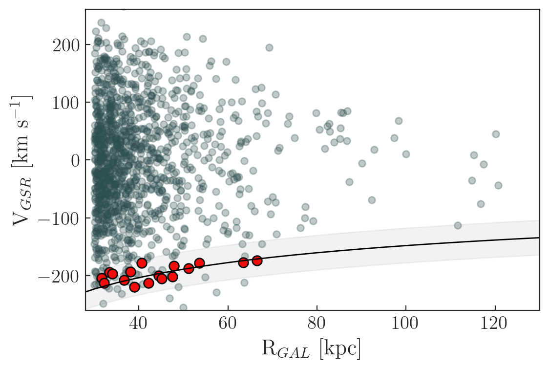
Figure 1: Selection of candidate H3 stream stars. All H3 stars with R${}_{GAL}>30$ kpc, FLAG = 0, SNR $>2$, Sgr_FLAG = 0, and coldstr = 0 are plotted as gray circles. Our kinematic selection criteria is represented by the shaded area and encompasses stars on orbits of similar total energy in a 10¹² M_⊙ NFW potential that represents the MW. The 17 stars satisfying this and the other selection criteria described in the text are shown as red circles and comprise our H3-selected sample. Distance uncertainties in H3 are estimated at $\sim 10$% and radial velocity uncertainties are smaller than or comparable to the plotted symbols.

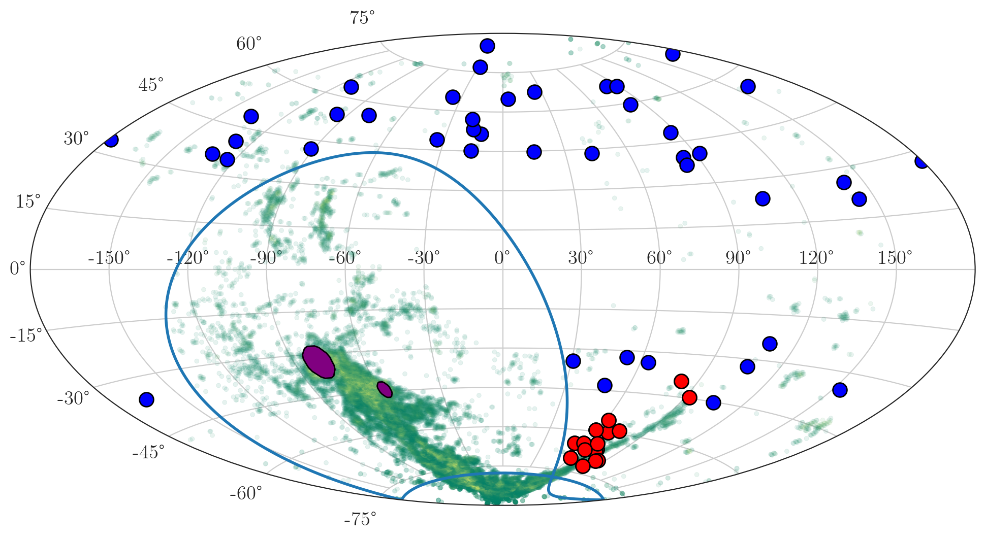
Figure 2: All-sky distribution in Galactic coordinates of the gaseous Magellanic Stream (Nidever et al., 2008a) in green, the LMC and SMC in blue ellipses, the H3-selected stars that satisfy all of our criteria in red, and those that satisfy all of our criteria except for the one related to the MS coordinate system in blue. The footprint of the H3 survey, which lies outside the enclosed region and avoids the Galactic disk, precludes us from finding stars along the MS that are closer to the Clouds than those shown.

2.2 Gaia Downselect

Our approach will work only if the properties of the H3-selected stars, which have precise radial velocity and distance estimates, are sufficiently distinct within the parameter set measured by Gaia that does not include these measurements to enable us to select corresponding stars. Fortunately, our selected set of stars is both fairly consistent in its proper motion values and colors and distinct from the underlying population of stars (Figure 3). First, we apply the basic parallax cut imposed in H3 ($\varpi<0.4$ mas yr^-). Then, we define our initial selection in proper motion to include most of the H3-selected stars: $0.0<\mu_{\alpha}/({\rm mas\ yr})^{-1}<1.05$ and $-1.5<\mu_{\delta}/({\rm mas\ yr})^{-1}<0.0$. We will trim more aggressively later but opt here to allow for some variation in proper motions among potential stream populations. In color-magnitude space we use the Gaia photometry and select stars with $16.6<G<18.5$ and $C<BP-RP<1.3$, where $C\equiv(39.4-G)/19.0$. Lastly, guided again by the H3-selected sample, we draw from the Gaia DR3 catalog only stars with MS coordinates ($l_{MS},b_{MS}$) such that $-115^{\circ}<l_{MS}<-65^{\circ}$ and $-20^{\circ}<b_{MS}<10^{\circ}$ to search for any existing population that closely tracks both the MS and the H3-selected stars.

The resulting population of 3,982 stars is presented in Figure 4 showing both $\mu_{\alpha}$ and $\mu_{\delta}$ as a function of $l_{MS}$. It is evident that 1) the distribution of stars is not uniformly distributed in proper motion, 2) there is a concentration of Gaia stars at $-75^{\circ}\lesssim l_{MS}\lesssim-95^{\circ}$ that matches the H3 stars to a tighter degree than allowed for by our proper motion selection cuts, and 3) there is a continuing population of stars toward more negative $l_{MS}$ that trends to lower values of $\mu_{\delta}$.

The selected stars can be divided into two sub-populations. The first is a set that matches that identified initially in H3. The correspondence between the H3-selected stars and these Gaia-selected stars supports the interpretation of the H3-selected stars as a coherent, physical stellar population and greatly increases the number of such stars. The second is a population that clusters farther along the MS, at more negative $l_{MS}$. This population is difficult to interpret because increasingly negative values of $l_{MS}$ corresponds to decreasing Galactic latitude, longer sightlines through the halo, and therefore more noise/contamination. Nevertheless, we do not yet dismiss this population entirely. We will return to this population later.

We use these results to refine our selection of Gaia stars that correspond to the H3-selected sample. We tighten our proper motion selection to $0.1<\mu_{\alpha}/({\rm mas\ yr}^{-1})<0.7$ and $-0.9<\mu_{\delta}/({\rm mas\ yr}^{-1})<-0.2$. In making these cuts we aimed for the following: 1) to retain as many of the H3-selected stars that overlap with the coincident, localized overdensity of Gaia stars, and 2) to exclude other overdensities, particularly the one at $l_{MS}\sim-100^{\circ}$, that do not have corresponding significant populations of H3-selected stars.

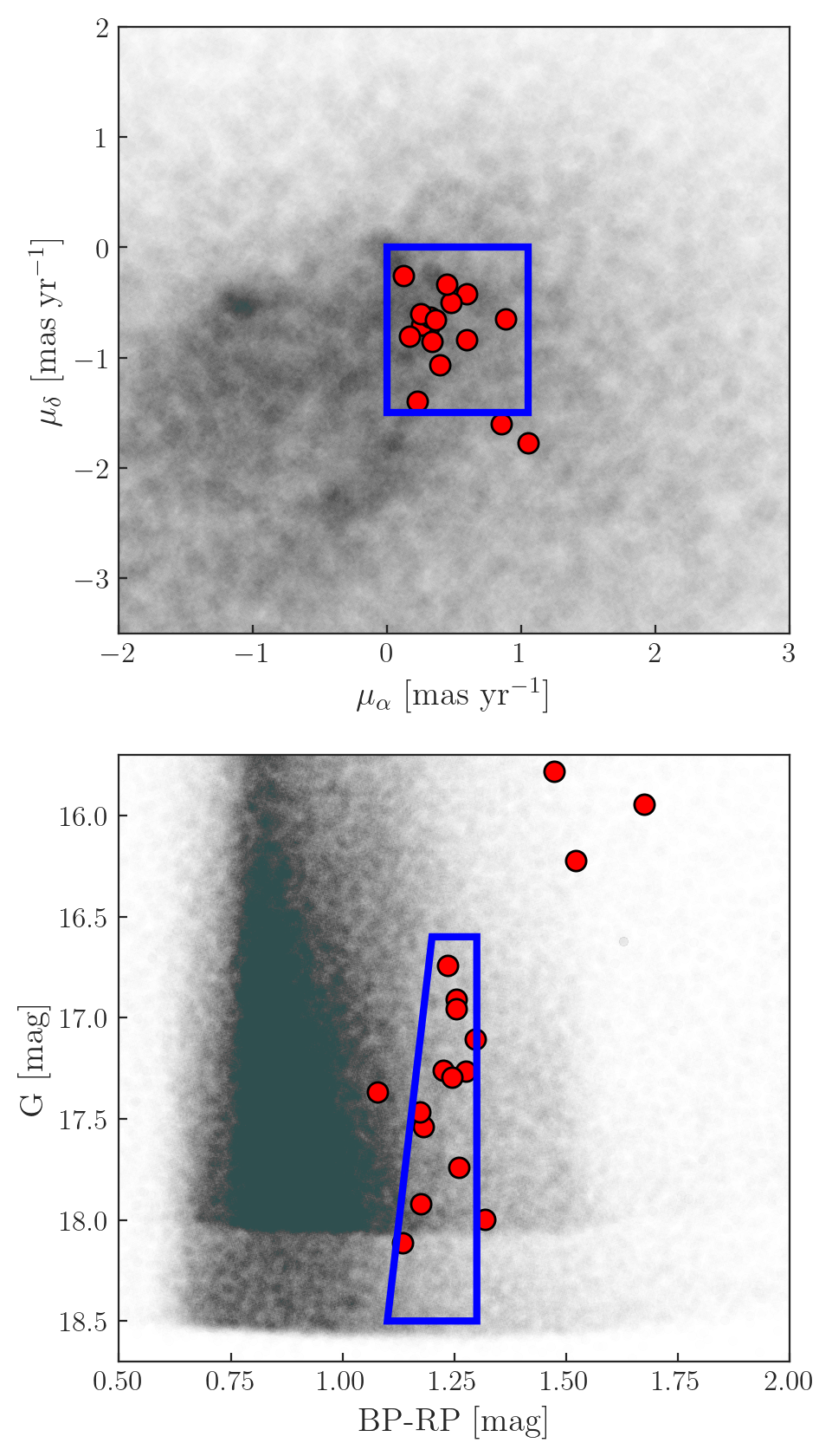
Figure 3: The H3-selected stars (red circles) are localized relative to the full H3 sample in Gaia proper motion coordinates and color-magnitude space. Blue outlines mark our selection boxes.

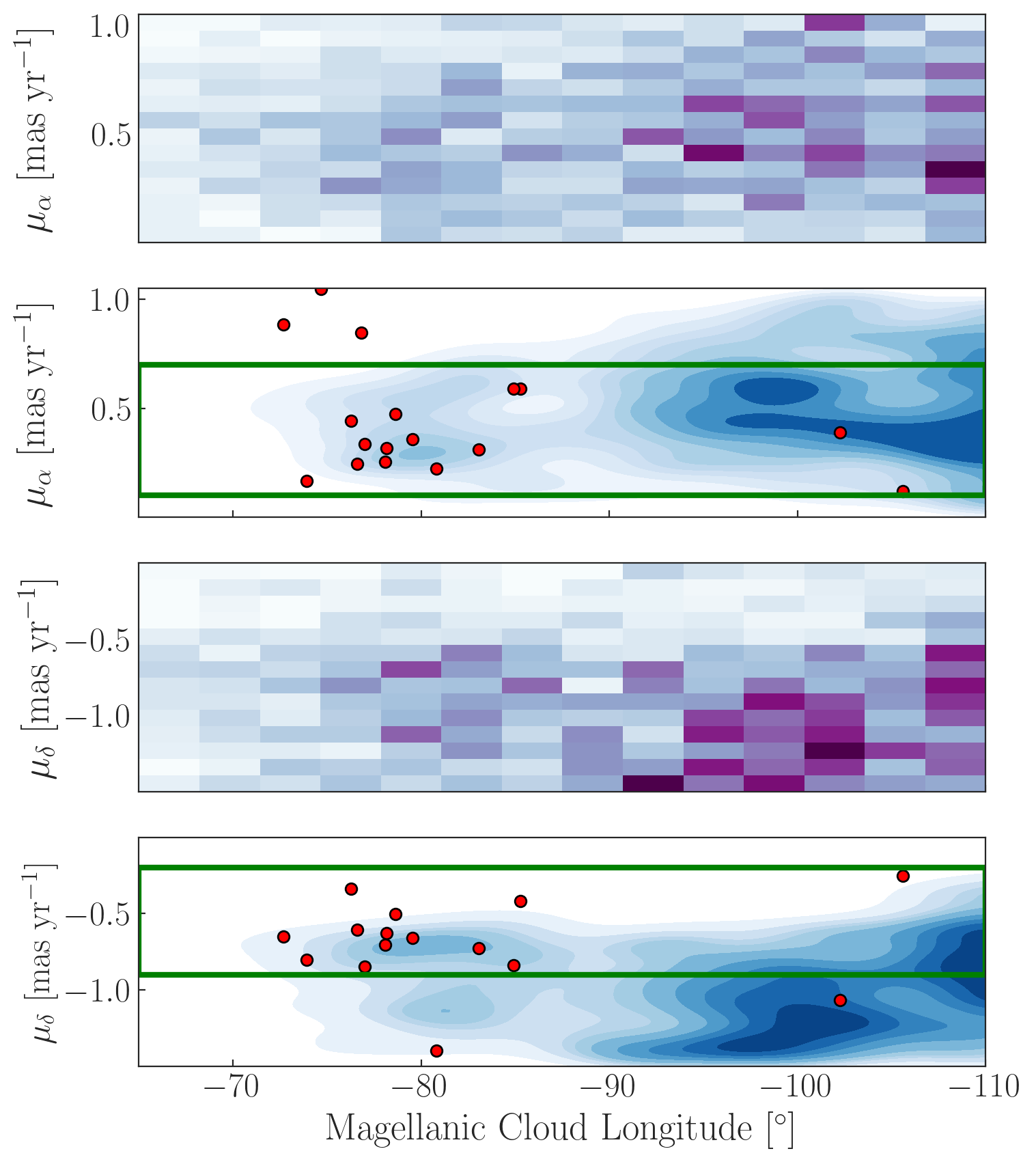
Figure 4: The distribution of proper motion values for stars selected using the criteria shown graphically in Figure 3 as function of MS longitude. For $\mu_{\alpha}$ and $\mu_{\delta}$ we show both the raw binned distribution and the smoothed distribution in blue. The H3-selected stars are superposed on the smoothed Gaia distributions as red circles. Green horizontal lines show our refined proper motion selection criteria. Stars between the two green lines are retained to produce Figure 5.

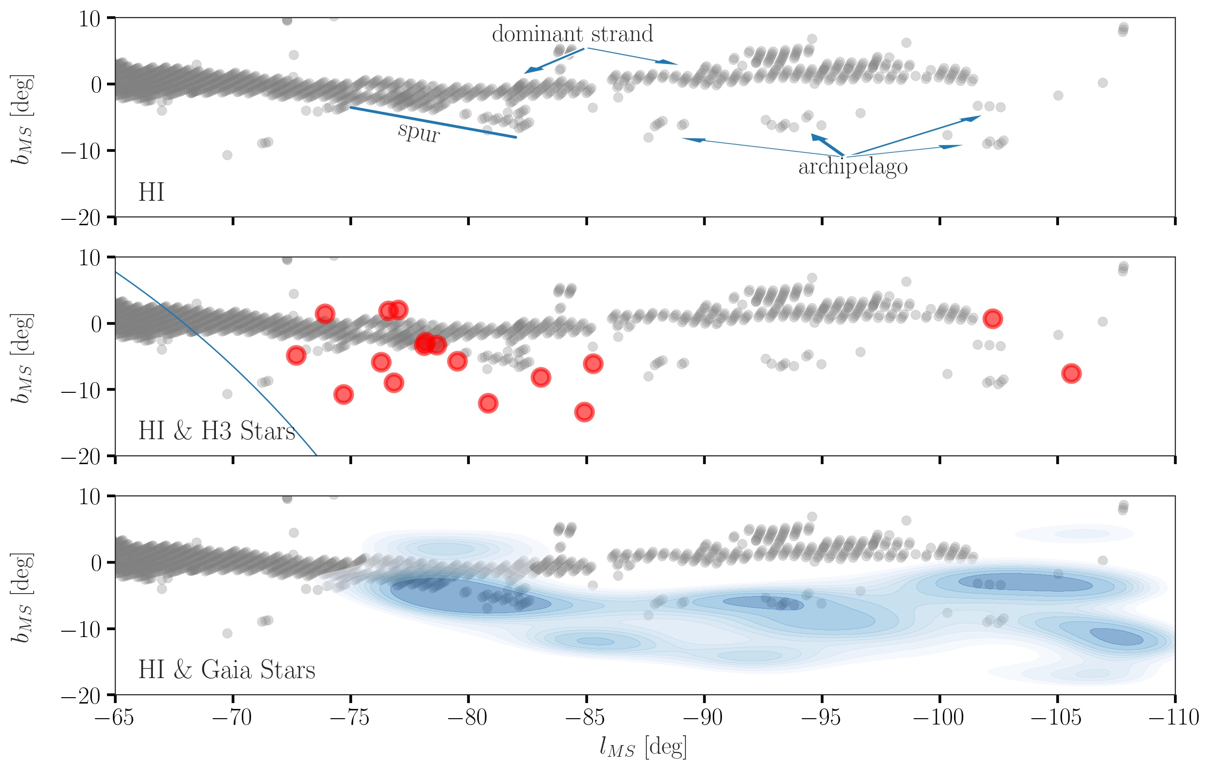
Figure 5: Three views of a Magellanic Stream system. Top panel presents the HI distribution along the Magellanic Stream in Stream coordinates (Nidever et al., 2008a). Note the bifurcation of the Stream at $l_{MS}\sim-75^{\circ}$ with a small spur to lower $b_{MS}$ that plausibly extends, through a set of small clouds that we name the “archipelago”, out to $l_{MS}\sim-105^{\circ}$. The data are presented discretely and so the gas, despite presumably being spatially diffuse, is plotted as discrete points. Middle panel adds to this picture of the gaseous Stream the H3-selected stars (red circles) that appear to deviate from the principal Magellanic Stream and follow the spur. The curved line represents the edge of the H3 survey footprint. Bottom panel adds to this picture the Gaia-selected stars. The distribution of selected stars, smoothed as in Figure 4, clearly follows the spur and perhaps, with less certainty, traces the HI archipelago all the way to $l_{MS}\sim-105^{\circ}$.

3 Results

The populations of gas, H3-selected stars, and our final set of Gaia-selected stars are presented in Figure 5. As noted previously, the MS is a set of apparently intertwined filaments (Cohen, 1982; Morras, 1983; Putman et al., 2003b; Nidever et al., 2008a). Because we do not know the distances to the various filaments, the 3-D geometry, and therefore the origin of the structures, is unclear. Nevertheless, in the upper panel of the Figure there appear to be at least two clear strands of the MS over the values of $l_{MS}$ included in the Figure. The dominant strand appears to be one that extends from at least $l_{MS}=-65^{\circ}$ to $l_{MS}\sim-85^{\circ}$, after which there is a slight gap with the plausible continuation of gas extending from $l_{MS}\sim-86^{\circ}$ to $l_{MS}\sim-102^{\circ}$. There is a second strand that bifurcates from the dominant strand at $l_{MS}\sim-75^{\circ}$, forms a spur and dives to lower value of $b_{MS}$. This strand plausibly continues along an “archipelago” of HI clouds stretching out as far as the dominant stream but mostly at more negative values of $b_{MS}$ than the dominant Stream (i.e. at $b_{MS}\sim-5^{\circ}$). We will refer to this strand as the subdominant one. We note for completeness, but do not show in this Figure, that the situation is even more complicated because the dominant stream itself shows a velocity discontinuity at the gap (Nidever et al., 2008b).

In the middle panel of the Figure we compare the gas to the distribution of the H3-selected stars. As suggested by Z20, the stars appear to be more closely associated with the subdominant MS strand, in particular with the spur to lower $b_{MS}$ at $-83^{\circ}\lesssim l_{MS}\lesssim-75^{\circ}$. In addition, one or both of the H3 stars at $l_{MS}<-100^{\circ}$ might be part of the extension of this population. As already noted, the small number of stars in the main group of H3-selected stars (15) makes it difficult to reach a definitive conclusion and motivated our study of the Gaia catalog.

In the lowest panel of the Figure we show the resulting distribution of the Gaia-selected stars (smoothed kernel density estimation). Our principal result is that we confirm that there is a population of stars that follows the HI spur that was initially associated with the H3-selected stars (i.e. the feature extending over $-83^{\circ}<l_{MC}<74^{\circ}$). It is evident that these Gaia-selected stars follow the subdominant strand rather than the dominant one. For reference, over the longitude range covered by the 15 H3-selected stars ($-86^{\circ}<l_{MC}<-74^{\circ}$) there are 297 Gaia-selected stars, which alleviates any concern that the H3-selected stars are themselves dominating the feature seen in the Gaia-selected stars.

There are additional concentrations of Gaia-selected stars that trace the HI archipelago noted previously. Although suggestive, the lack of H3-selected stars along the archipelago prevents us from using kinematics or distances to confirm that these are a physical continuation of the subdominant MS strand. These regions are within the H3 footprint, so a relevant question is why H3 identified at most only two of the stars in these features. Perhaps we were somewhat unlucky, although these are also less populated features among the Gaia stars, or perhaps the corresponding stars are at larger distance and hence more challenging for H3. Follow-up spectroscopy of the Gaia-selected stars in these features is an obvious way forward.

We searched other datasets for existing observations of stars in this area of sky. In particular, using the distance estimates provided by Anders et al. (2019), we searched in each of the datasets they provide for stars within this region of sky that have 16% percentile distance estimates that are $>$ 30 kpc. We find 7 matches in the Starhorse LAMOST (Cui et al., 2012) LRS DR7 catalog and 18 in their SDSS DR12 catalog (Alam et al., 2015). In neither case do the stars clearly delineate a feature that corresponds to the MS. While there are stars in these samples that are plausibly associated with the Gaia features we have identified, we can reach no clear conclusions with these small samples.

We return now to the most significant overdensity in Figure 4, which is at $l_{MS}\sim-100^{\circ}$. To investigate this feature, we match the Gaia-selected stars with $l_{MS}<-90^{\circ}$ and $\mu_{\delta}<-0.9$ to the H3 catalog. We find 17 stars in common. Unlike the original set of H3-selected stars, these have a wide range of radial velocities ($-230<v_{GSR}$/(km s${}^{-1})<100)$ and so do not appear to be a true physical concentration. We close by again noting that as $l_{MS}$ becomes more negative in Figure 4 one is approaching the Galactic plane, a trend which may be responsible for the larger fluctuations toward the right side of Figure 4.

To further examine this issue, and to provide a control for the detection of the stellar populations at more positive values of $l_{MS}$, we apply the same selection cuts to a mock Gaia catalog of halo stars with $G<19$ mag created using GUMS (Isasi et al., 2010). We present the analogous figure to the lowest panel of Figure 5 in Figure 6. We do indeed find, as speculated, larger fluctuations in the stellar projected densities at more negative values of $l_{MS}$. As a cautionary note, without distance or radial velocity information the largest density fluctuation could be incorrectly identified as a stellar population associated with the tip of the MS. This confusion is not an issue at less negative values of $l_{MS}$, particularly at $l_{MS}\sim-80^{\circ}$ where we identify our most significant cluster of Gaia-selected stars, because the random fluctuations in this region are negligible. Additionally, we remind the reader that for the H3 stars that correspond to this feature we do have velocity information confirming that this is a physically coherent set of stars. For the clusters of Gaia-selected stars apparently associated with the HI archipelago, we stress the tentative nature of that association and the need for follow-up spectroscopy of candidates.

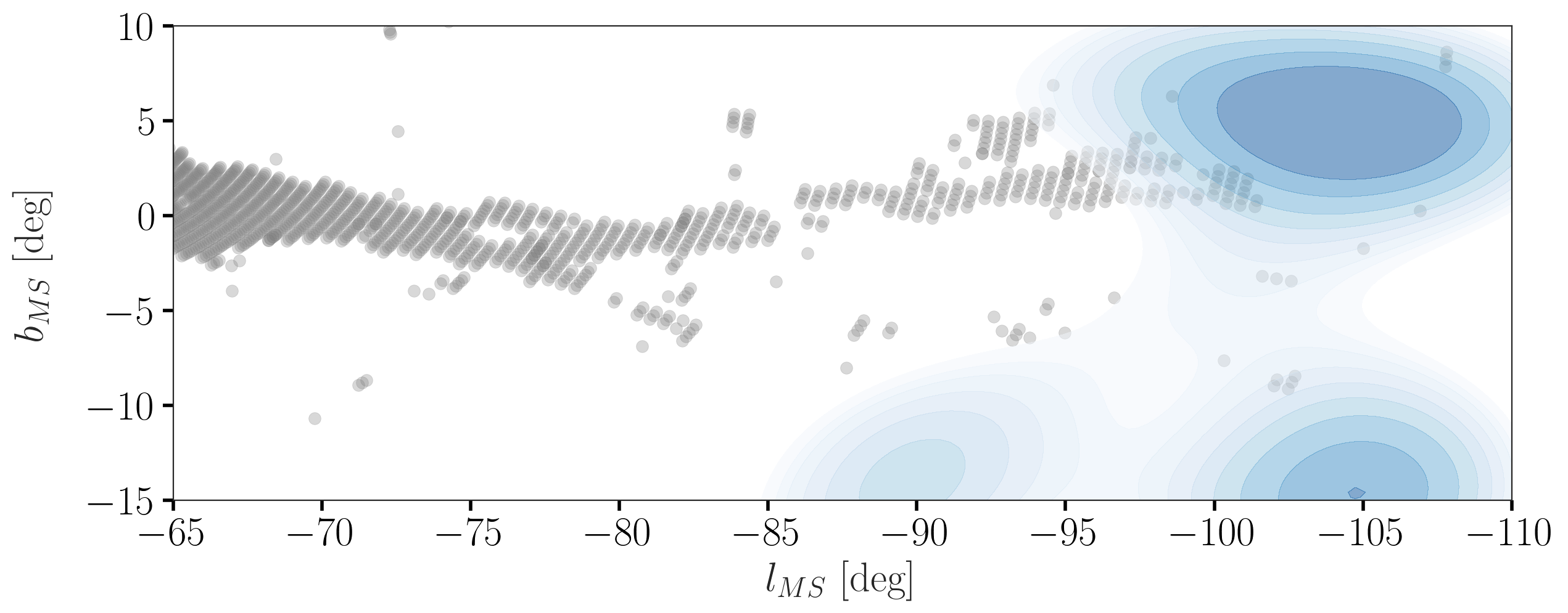
Figure 6: The resulting distribution of simulated halo stars selected in the same manner as the Gaia stars shown in Figure 5. As anticipated, larger fluctuations appear at most negative values of $l_{MS}$.

We now return to the question of potential cross-contamination with the population of H3 stars identified as Sgr members (i.e. those with Sgr_FLAG = 1). We noted in §2 that 5 members of the Z20 sample are now labeled as Sgr members in the H3 catalog and so rejected from our current analysis. If we redo our selection using only labeled Sgr members in H3 we find 6 stars, in other words only one additional star. This set of six is a much more heterogeneous population of stars than our sample. Three of these are well outside the color-magnitude bounds we used for the Gaia-selected stars, the stars do not track the HI spur, they have a wide range in [Fe/H] (from $\sim-2.4$ to $-$1.0), and all but one lie outside the proper motion bounds set in Figure 4. We conclude that Sgr stars, at least those similar to those identified as such in H3, are not the bulk of our sample and that we have not missed a large number of stream stars due to an incorrect classification as Sgr stars.

Finally, in closing we return to the H3-selected stars. To even more finely select stars corresponding to the Gaia-selected population, we now apply the final proper motion and photometric cuts to the H3-selected stars that we applied when selecting the Gaia stars. This results in the rejection of 8 stars from the sample of 17. While this is a large fraction, the selection seems to be doing something sensible (Figure 7). First, it removes the four stars with the largest values of [Fe/H] and these happen to be quite consistent with the peak of the halo distribution in both [Fe/H] and [$\alpha$/Fe]. Second, it removes 7 of 9 of the stars with the highest values of [$\alpha$/Fe], again values that are more consistent with a halo population. The remaining stars have $\langle$[Fe/H]$\rangle=-1.48\pm 0.06$ and $\langle$[$\alpha$/Fe]$\rangle=0.06\pm 0.4$, which are consistent with the properties of SMC stars (De Propris et al., 2010; Hasselquist et al., 2021; Chandra et al., 2023). Although the trimming may be overly aggressive because we are applying our tightest proper motion cuts and because color and metallicity are dependent, this subsample is the closest H3 analog to the Gaia-selected population. The remaining stars are most consistent with an SMC origin, although they could be drawn exclusively from the metal-poor tail of LMC members. Alternatively, they could come from an unknown progenitor with chemical properties comparable to those of the SMC.

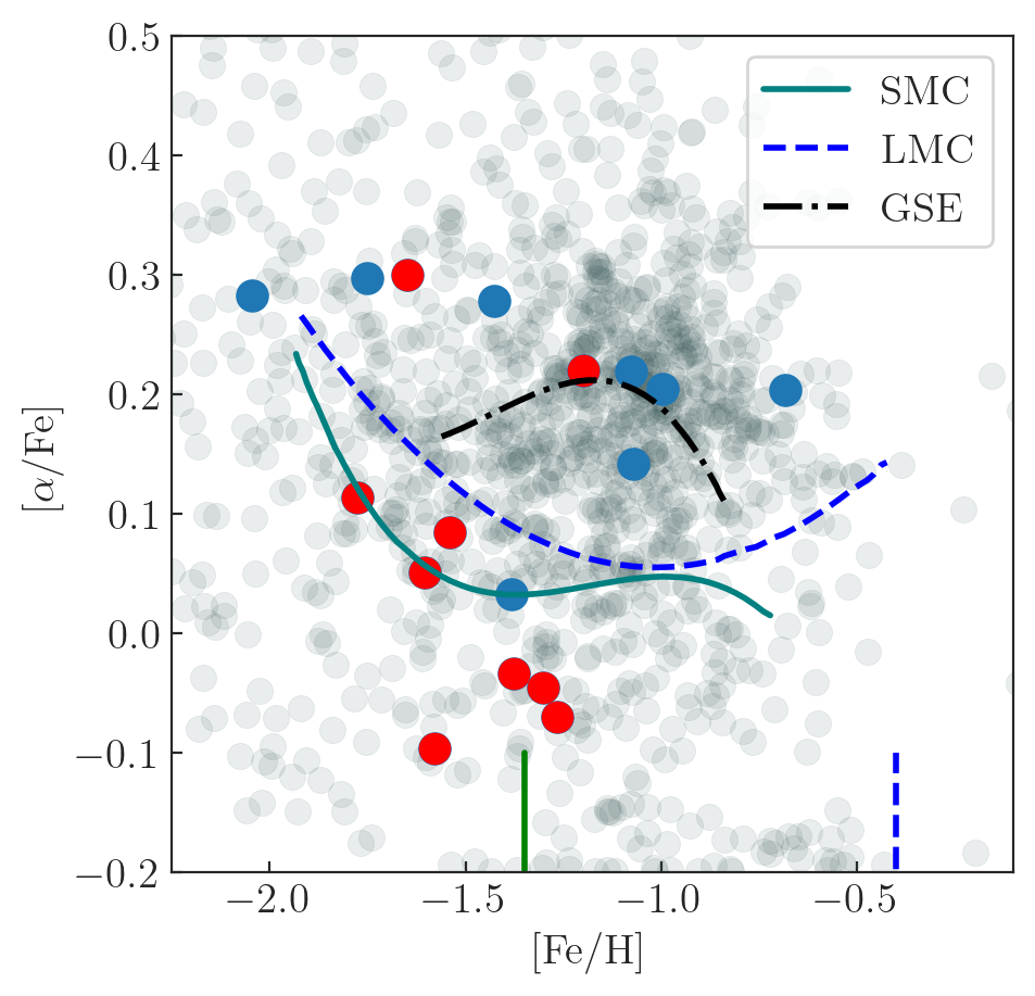
Figure 7: Chemical properties of H3-selected stars. We compare the properties of the H3 halo stars (gray), which satisfy all of our selection criteria except the kinematic and MS coordinate ones, to the H3-selected stars. In blue are those H3-selected stars that do not meet the criteria applied to the Gaia stars, while in red are those that do. We show tracks in abundance space for the stellar populations of three MW satellites (Hasselquist et al., 2021) and mean values of [Fe/H] for the SMC from De Propris et al. (2010) and the LMC from Cole et al. (2005).

4 Discussion

The nature of the dominant and subdominant MS strands is fundamentally different. The lack of stars from our dataset in the dominant strand — drawn either from H3 or Gaia — does not necessarily indicate that it does not contain stars. Both surveys are increasingly insensitive to stars at larger distances. The stars identified by C23 lie between $60-120$ kpc, and some may be associated with the dominant strand (Figure 8). If so, then the dominant and subdominant MS strands as we have identified them are separated by tens of kpc ($\sim 100$ kpc vs. 47 kpc) and are only closely aligned in projection. Such overlapping streams have been identified in simulations, either due to the overlapping of two separate tidal tails or the orbital wrapping of a single tail (Diaz & Bekki, 2012).

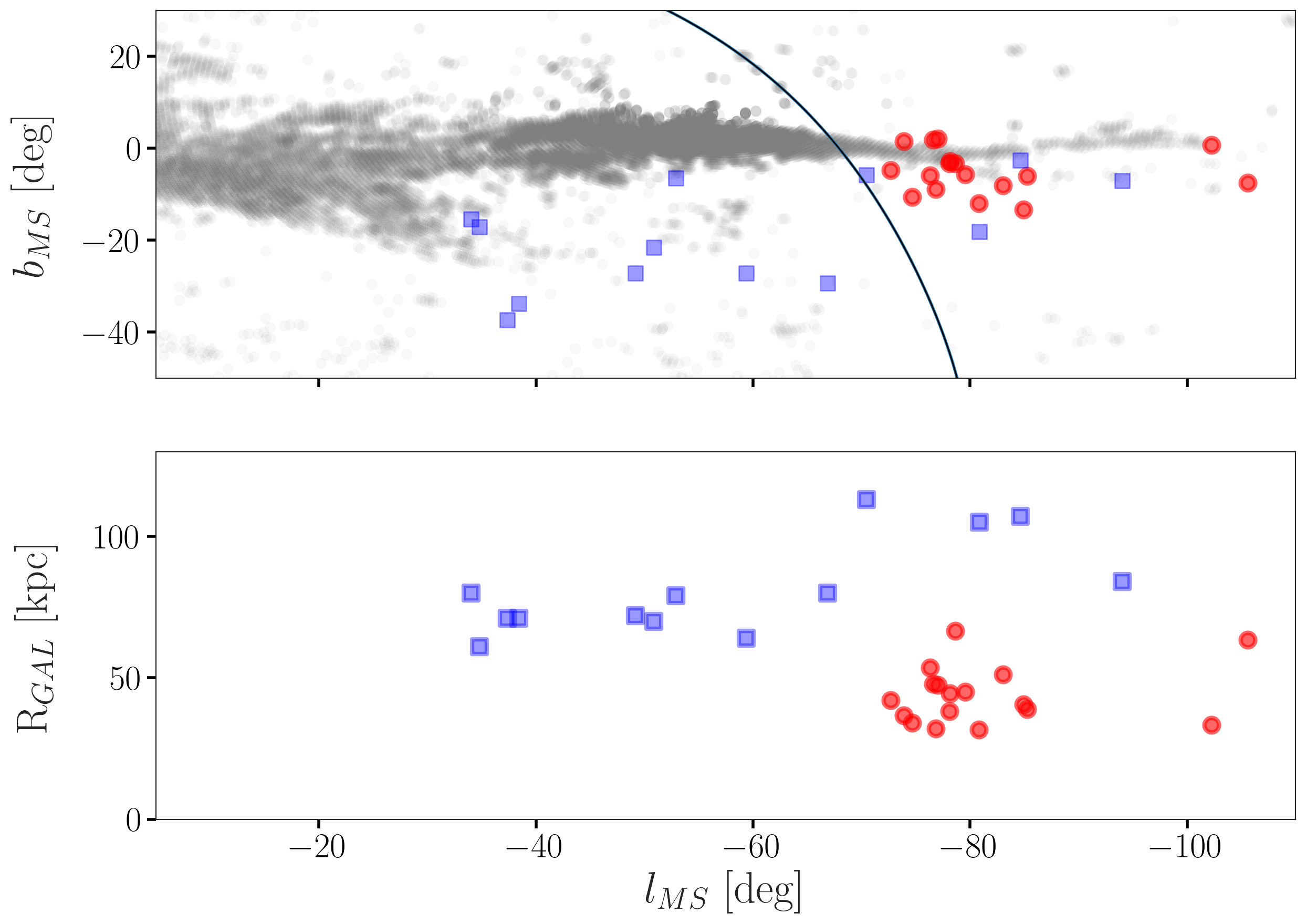
Figure 8: Comparison of our set of stars to those identified by C23. The C23 stars (blue squares) are distributed over a far larger area of sky than our stars (red circles) and so only three or four overlap our search area. Those that are projected near our set of stars are at about a factor of 2 farther away and therefore likely trace a different physical structure. They were also selected to have different angular momenta. We plot the HI distribution in the upper panel from Nidever et al. (2008b) and a curve showing the boundary of the H3 footprint for reference.

An alternative possibility is that the dominant strand is devoid of stars and arises either from tidally stripped gas that was originally at a radius beyond where there were many stars (Diaz & Bekki, 2012) or from gas that was blown out of the central galaxy and then stripped (Nidever et al., 2008b). In either version of this alternative scenario, the C23 stars are unrelated to this dominant strand of the MS and are likely tidal stellar debris drawn from the extremities of the Clouds. Such stellar halo-like components have been traced in the periphery of the Clouds (Belokurov & Erkal, 2019; El Youssoufi et al., 2021; Gaia Collaboration et al., 2021) and likely have a complicated history (e.g., Massana et al., 2024).

The subdominant MS strand investigated in the present work shows a close correspondence between stars and gas in the detailed density structure along the filament. The presence of stars confirms that this gaseous filament is a tidal feature. The correspondence between gas and stars suggests that material originated from a galactic disk, which would contain both gas and stars. The metallicity and $\alpha$ enrichment of our H3-selected stars is consistent with an SMC origin, although more complex scenarios cannot be definitively excluded.

To expand on this point, consider that in $\S$3 we argue that the stellar population within the subdominant strand of the MS does not seem related to Sgr stream stars in the H3 dataset. However, it remains plausible that an additional, hitherto undetected component of the Sgr stream could contribute stars matching the population presented here. In particular, the simulations of Vasiliev et al. (2021) — which are constrained to match observations of the main stream body — predict early-stripped debris that are similarly offset from the stream track as the stars considered here. Although we consider this specific scenario to have low probability given the correspondence of our identified stars with the MS gas, the limited footprint of the (northern) H3 Survey prevents us from investigating whether the population studied here extends closer to the Sgr stream (see Figure 8). Forthcoming surveys — chiefly the fifth-generation Sloan Digital Sky Survey from the southern hemisphere (SDSS-V; Kollmeier et al. 2017) — should be capable of resolving this question.

5 Conclusions

Using an H3-selected sample of stars that corresponds to the population identified by Z20 as a potential stellar counterpart to the gaseous Magellanic Stream (MS), we utilized the Gaia catalog to expand the number of known stars in this component and to map this population. We find that the MS consists of at least two different strands. The dominant one, as defined by gas content, is devoid of stars with Galactocentric distances $\lesssim 55$ kpc and may be traced by stars at larger distances (C23). The subdominant one shows a close correspondence between stars and gas and lies at distances $\lesssim 55$ kpc. This finding demonstrates conclusively that this feature, at least, is tidal in origin. Given the association between gas and stars, and the mean metallicity of the stars, we suggest that it is tidal material drawn from the disk of the SMC. Of course, more surprises (e.g. Nidever, 2024) are likely to come in the study of the intriguing, complex Magellanic system.