Safe Multi-Agent Reinforcement Learning with Convergence to Generalized Nash Equilibrium

Abstract

Multi-agent reinforcement learning (MARL) has achieved notable success in cooperative tasks, demonstrating impressive performance and scalability. However, deploying MARL agents in real-world applications presents critical safety challenges. Current safe MARL algorithms are largely based on the constrained Markov decision process (CMDP) framework, which enforces constraints only on discounted cumulative costs and lacks an all-time safety assurance. Moreover, these methods often overlook the feasibility issue—where the system will inevitably violate state constraints within certain regions of the constraint set—resulting in either suboptimal performance or increased constraint violations. To address these challenges, we propose a novel theoretical framework for safe MARL with state-wise constraints, where safety requirements are enforced at every state the agents visit. To resolve the feasibility issue, we leverage a control-theoretic notion of the feasible region, the controlled invariant set (CIS), characterized by the safety value function. We develop a multi-agent method for identifying CISs, ensuring convergence to a Nash equilibrium on the safety value function. By incorporating CIS identification into the learning process, we introduce a multi-agent dual policy iteration algorithm that guarantees convergence to a generalized Nash equilibrium in state-wise constrained cooperative Markov games, achieving an optimal balance between feasibility and performance. Furthermore, for practical deployment in complex high-dimensional systems, we propose Multi-Agent Dual Actor-Critic (MADAC), a safe MARL algorithm that approximates the proposed iteration scheme within the deep RL paradigm. Empirical evaluations on safe MARL benchmarks demonstrate that MADAC consistently outperforms existing methods, delivering much higher rewards while reducing constraint violations.

1 Introduction

Cooperative multi-agent reinforcement learning (MARL) has drawn substantial research attention, driven by the increasing demand for effective coordination among intelligent machines [1, 2]. Agents in a cooperative MARL system collaborate with each other to pursue a joint objective, operating in a shared environment where each agent’s decisions impact the entire team. To tackle the non-stationarity challenge of one agent’s updates affecting others, the centralized training decentralized execution (CTDE) paradigm has been developed [3, 4]. In the CTDE framework, the algorithm has access to global information across all agents during the training phase, after which the trained agents are prepared to make independent decisions for deployment. Significant advancements have been made in this area, both in theory [5, 6, 7, 8, 9] and applications [10, 11, 12, 13].

Despite the remarkable achievements in MARL algorithms, most of them are primarily designed to maximize rewards and achieve optimal performance. However, real-world deployments demand that agents operate within specific constraints, i.e., ensuring safety. In practice, safety enforcement should take precedence over performance optimization. For example, in the context of autonomous driving, vehicles must follow traffic rules and avoid collisions under all circumstances, prioritizing safety above all else. While safe RL has been extensively studied in the single-agent setting [14], the safe MARL problem remains quite challenging. That is largely due to the fact that in the multi-agent setting, both the objective and the constraints are influenced by the decisions of all agents. There are multiple points of tension that could destabilize the learning process, including the inherent conflict between reward maximization and constraint satisfaction, as well as disagreements in updating directions across agents that could violate the shared constraints.

Pioneering works in safe MARL theory include [15, 16, 17, 18, 19, 20]. Despite the significant progress, there are notable limitations with existing safe MARL methods. First, many algorithms, such as Safe Dec-PG [16], MACPO and MAPPO-Lagrangian [17] are grounded in the constrained Markov decision process (CMDP) framework [21], in which the objective is to maximize total rewards while ensuring that the expected trajectory costs remain below a predefined threshold. However, in real-world applications, safety constraints must be enforced at every time step, rather than just on average, as any violation could lead to catastrophic consequences [14]. Second, existing methods rarely consider the feasibility issue, i.e., wherein no policy can keep the system persistently safe for certain states within a subset of the constraint set [22]. Identifying the feasible region is critical for safe RL algorithms, as optimizing rewards over infeasible regions is ill-posed and can lead to unstable training [23, 24]. Additionally, a larger feasible region provides a broader operational space for the agents, leading to better performance. Third, it is particularly challenging to coordinate the updates of multiple agents to ensure joint constraint satisfaction while still improving overall performance. Since each agent’s update alters the set of feasible directions for the others, the update mechanism must be carefully designed to ensure that agents collaboratively converge to a safe and performant equilibrium. Existing methods often struggle to balance constraint satisfaction with task performance, resulting in either suboptimal outcomes or increased violations of safety constraints.

To address the aforementioned challenges, this paper introduces a novel theoretical framework for handling feasibility and optimality in safe MARL with state-wise constraints. Unlike the CMDP setting commonly used in existing studies, which imposes trajectory-wise constraints, we focus on a stricter safety formulation where agents must satisfy constraints at every state they visit. For identification of feasible region, we utilize the concept of controlled invariant set in control theory, characterized by the safety value function from Hamilton-Jacobi reachability analysis [22, 25]. Inspired by the one-agent-at-a-time policy improvement technique [6, 7, 8, 9], we propose a MARL approach for the identification of controlled invariant sets, which ensures convergence to a Nash equilibrium on safety value function. By leveraging action-space constraints derived from these controlled invariant sets, we develop a multi-agent dual policy iteration algorithm for constrained cooperative Markov games. The objective is two-fold: for states within the maximal identifiable controlled invariant set, agents aim to maximize the joint rewards, whereas, for states outside this set, the focus shifts to minimizing constraint violations. The proposed iteration scheme employs two individual policies for each agent—one dedicated to achieving the two-fold objective and the other for collaboratively learning the controlled invariant sets. Our methods enable agents to obtain the highest rewards possible while ensuring safety, thereby striking an optimal balance between task performance and constraint satisfaction (i.e., generalized Nash equilibrium). The key contributions of this paper are summarized as follows.

• We propose a MARL approach for identifying controlled invariant sets of nonlinear dynamical systems. Our method ensures convergence to a Nash equilibrium on the safety value function, achieving local optimality in finding feasible regions within the multi-agent setting.

• We introduce the multi-agent dual policy iteration algorithm, which, to the best of our knowledge, is the first safe MARL algorithm with guaranteed convergence to a generalized Nash equilibrium on state-wise constrained cooperative Markov games. The key insight is to transform state constraints into state-dependent action spaces, which allows optimizing task performance across all feasible directions in an agent-by-agent manner, despite the inherent non-stationarity in safe MARL problems.

• We propose multi-agent dual actor-critic (MADAC), a safe MARL algorithm that approximates the proposed iteration scheme within the deep RL context. Empirical evaluations on safe MARL benchmarks demonstrate that MADAC consistently outperforms existing methods, delivering much higher rewards while reducing constraint violations.

2 Related Work

Safe RL has been extensively studied in the single-agent setting. There are mainly two types of safety formulation in safe RL algorithms: trajectory-wise safety and state-wise safety. The former requires that the expected trajectory cost remains below a certain threshold (the CMDP framework [21]), while the latter enforces constraints at every state the agents visit [14]. For trajectory-wise safety formulation, algorithms typically employ the Lagrange method or trust region method to perform constrained policy optimization. Ha et al. [26] enhance the soft actor-critic algorithm by adding Lagrange multipliers and performing dual ascent on the Lagrangian. Chow et al. [27] introduce constraints on the conditional value-at-risk of cumulative costs and design corresponding policy gradient and actor-critic algorithms. Achiam et al. [28] propose the constrained policy optimization algorithm with guarantees for near constraint satisfaction at each iteration. Zhang et al. [29] update policy in the nonparameterized policy space and then project the updated policy back into the parametric policy space. For state-wise safety formulation, the key is to achieve set invariance with control-theoretic tools such as Hamilton-Jacobi reachability [22, 30], control barrier function [31], and safety index [32]. Ma et al. [33] jointly optimize the control policy and the neural safety index. Yu et al. [23] jointly learn the safety value function and the control policy. Li et al. [24] propose a dual policy iteration algorithm that converges to the maximal robust invariant set and optimal task policy simultaneously. Wang et al. [34] propose a robust safe RL algorithm that guarantees local convergence to a minimax equilibrium solution. State-wise safety has also been explored from optimization perspectives. Zhao et al. [35] propose state-wise constrained policy optimization, demonstrating that the algorithm achieves bounded worst-case safety violations in state-wise constrained MDPs.

Safe MARL is an emerging research area that has been gaining increasing attention. Lu et al. [16] propose a decentralized policy gradient approach for constrained policy optimization with networked agents and prove the algorithm converges to a first-order stationarity point for the formulated problem. Melcer et al. [15] address the shielded reinforcement learning problem in the multi-agent setting and present an algorithm for the decomposition of a centralized shield. Gu et al. introduce trust region optimization techniques that ensure monotonic improvement in rewards while satisfying safety constraints at every iteration. They also present two algorithms (MACPO and MAPPO-Lagrangian) for practical deployment in high-dimensional environments [17]. Zhao et al. [20] update policies by solving a constrained optimization problem in the non-parameterized policy space and then projecting the solution into the parametric policy space. Ding et al. [18] propose a provably efficient algorithm for solving episodic two-player zero-sum constrained Markov games. Ying et al. [19] present a primal-dual approach for safe MARL problems, where the objective and constraints are defined by general utilities, and prove its convergence to a first-order stationary point. Our work differs from existing methods in several key aspects. First, we consider a stricter safety requirement that enforces constraints at every state the agents visit, contrasting with the trajectory-wise safety formulation (the CMDP framework) employed in [16, 17, 20, 18, 19]. Second, we address the feasibility issue inherent in safe RL problems [23, 24]. Our algorithm automatically identifies the feasible region and adjusts to different objectives based on the state’s feasibility, whereas existing methods [16, 17, 20, 18, 19] generally assume initial feasibility. Third, although the algorithm in [17] achieves performance improvement and constraint satisfaction at each iteration, no convergence guarantee is provided. Our method ensures convergence to a generalized Nash equilibrium, where no agent can enhance the objective by unilaterally modifying their policy within all feasible directions.

3 Multi-Agent Dual Policy Iteration

In this section, we introduce the multi-agent dual policy iteration algorithm for state-wise safe MARL. We first develop a multi-agent approach to identify controlled invariant sets for nonlinear systems, which plays a critical role in the following formulation and analysis. Next, we provide a formal problem formulation for state-wise constrained cooperative Markov games, specifying the objective and constraints. Finally, we present the iteration scheme and establish its convergence to a generalized Nash equilibrium for the constructed problem.

For simplicity of exposition, we will consider finite state and action spaces. Our results extend to general compact spaces. We have the following definition.

Definition 1 (State-wise Constrained Cooperative Markov Game).

A state-wise constrained cooperative Markov game is represented by a tuple $\mathcal{M}=\left(\mathcal{N},\mathcal{X},\mathcal{U},f,r,h,\gamma,\gamma_{h},d\right)$, where $\mathcal{N}=\{1,2,\dots,n\}$ denotes the set of $n$ agents, $\mathcal{X}$ denotes the state space, $\mathcal{U}=\prod_{i=1}^{n}\mathcal{U}_{i}$ is the joint action space (as the product of individual action spaces), $f:\mathcal{X}\times\mathcal{U}\rightarrow\mathcal{X}$ denotes the deterministic system dynamics, $r:\mathcal{X}\times\mathcal{U}\rightarrow\mathbb{R}$ is the reward function, $h:\mathcal{X}\rightarrow\mathbb{R}$ is the constraint function, $\gamma\in(0,1)$ denotes the reward discount factor, $\gamma_{h}\in(0,1)$ denotes the safety discount factor, and $d$ denotes the initial state distribution.

Note that the safety discount factor $\gamma_{h}$ is introduced specifically for algorithms addressing safety, which will be explained later. Given a state $x\in\mathcal{X}$, each agent individually selects an action $u_{i}\in\mathcal{U}_{i}$. An individual policy is denoted by $\pi_{i}:\mathcal{X}\rightarrow\mathcal{U}_{i}$, and $u_{i}=\pi_{i}(x)$. The joint action of all agents is denoted by $u=(u_{1},u_{2},\cdots,u_{n})\in\mathcal{U}$. The joint policy is expressed as $\pi=\prod\pi_{i}$, and thus $u=\pi(x)$.

Since our method involves operations on the actions and policies of a subset of agents, the following notation is introduced. An ordered subset of $\mathcal{N}$, $\left\{i_{1},i_{2},\cdots,i_{m}\right\}$, is denoted as $i_{1:m}$, and its complement by $i_{-1:m}$. The joint policy of agents $i_{1:m}$ is denoted by $\pi_{i_{1:m}}$, and their joint action by $u_{i_{1:m}}$.

3.1 Identification of Controlled Invariant Set

As discussed earlier, a key fact from control theory is that, given a constraint set, only a subset of it can be controlled to remain safe indefinitely, which is known as the controlled invariant set (CIS). Therefore, to design safe RL algorithms, it is essential to properly identify the CIS and to constrain the system state within the CIS rather than the full constraint set. Otherwise, when the system state leaves the CIS, it will inevitably violate the constraints regardless of the control inputs, thus causing the constrained policy optimization to be ill-conditioned.

Hamilton-Jacobi reachability analysis is a control-theoretic verification method for ensuring the safety of nonlinear systems. In this approach, the CIS is identified through the safety value function, which is the solution to the Hamilton-Jacobi-Isaacs partial differential equation (HJI-PDE) [22, 25]. However, solving the PDEs requires discretizing the state and action spaces, which leads to exponential scaling with increasing dimensions (the curse of dimensionality). Recently, RL approaches have been developed for Hamilton-Jacobi reachability, providing more tractable solutions for high-dimensional systems [36, 23, 24]. However, these methods are limited to single-agent systems, and it remains unclear how to extend them to multi-agent settings as well as providing convergence guarantees. We will address these gaps by proposing an agent-by-agent sequential update scheme for safety value functions. Given some safety requirements $h(x)\geq 0$, we define the safety value function and the controlled invariant set as follows.

Definition 2 (Constraint Set).

The constraint set is defined as the zero-superlevel set of constraint function $h(x)$:

$$S_{h}=\left\{x\in\mathcal{X}\mathrel{}\middle|\mathrel{}h(x)\geq 0\right\}.$$ (1)

Definition 3 (Safety Value Function [23, 24]).

Given a joint policy $\pi_{h}$ of all agents and $\gamma_{h}\in(0,1)$, the safety value function $V_{h}^{\pi_{h}}$ of this specific policy is defined as

$$\begin{gathered}V_{h}^{\pi_{h}}(x)=\min_{t\in\mathbb{N}}\left\{\gamma_{h}^{t+1}h\left(x_{t}\right)\right\}\\ \begin{aligned} \text{ s.t. \quad}&x_{0}=x,u_{t}=\pi_{h}\left(x_{t}\right),\\ &x_{t+1}=f\left(x_{t},u_{t}\right),t\geq 0.\end{aligned}\end{gathered}$$ (2)

Definition 4 (Controlled Invariant Set [24]).

If $\mathop{\max}\limits_{x\in\mathcal{X}}V_{h}^{\pi_{h}}(x)\geq 0$ for a joint policy $\pi_{h}$, the controlled invariant set of this specific policy is defined as

$$S_{\rm{c}}^{\pi_{h}}=\left\{x\in\mathcal{X}\mathrel{}\middle|\mathrel{}V_{h}^{\pi_{h}}(x)\geq 0\right\}.$$ (3)

The safety value function $V_{h}^{\pi_{h}}$ quantifies the level of risk associated with the system under a given policy $\pi_{h}$ by indicating the minimum constraint value of the infinite-horizon trajectory driven by $\pi_{h}$. The discount factor $\gamma_{h}$ is introduced to ensure that the safety value is the fixed point of a contraction mapping (which is defined in Lemma 1). Therefore, at any state that has a non-negative safety value, the system is guaranteed to remain safe under the policy $\pi_{h}$. This leads to the concept of controlled invariance, as stated in Definition 4, which we will further explore later.

Since $V_{h}^{\pi_{h}}$ is defined over the infinite horizon, it inherently follows a recursive structure arising from dynamic programming, referred to as the self-consistency condition [36, 23, 24].

Lemma 1 (Self-consistency Condition for Safety Value Function [23, 24]).

The safety value function $V_{h}^{\pi_{h}}$ satisfies

$$V_{h}^{\pi_{h}}(x)=\gamma_{h}\min\left\{h(x),V_{h}^{\pi_{h}}\left(f(x,\pi_{h}(x))\right)\right\}.$$ (4)

Furthermore, the safety self-consistency operator $\mathcal{T}_{h}^{\pi_{h}}$ defined as

$$\left[\mathcal{T}_{h}^{\pi_{h}}(V_{h})\right](x)=\gamma_{h}\min\left\{h(x),V_{h}\left(f(x,\pi_{h}(x))\right)\right\}$$ (5)

is a contraction mapping and $V_{h}^{\pi_{h}}$ is the unique fixed point of $\mathcal{T}_{h}^{\pi_{h}}$.

Remark 1.

Note that there are multiple ways to introduce the discount factor $\gamma_{h}$ in the safety value function, such as [36, 37, 38], leading to slightly different formulations of the self-consistency condition. For simplicity of presentation, we choose to omit the $(1-\gamma_{h})h(x)$ term commonly used in the literature [36, 23, 24] since the resulting form is still a contraction. We should note, however, that our proposed iteration scheme works with the other formulations.

Solving the operator equation (5) is essentially the policy evaluation step, in which we calculate the safety value function $V_{h}^{\pi_{h}}$ for a given policy $\pi_{h}$. Naturally, the next step is policy improvement. In the single-agent setting, this can be done as

$$\pi_{h}^{\rm{new}}(x) =\underset{u\in\mathcal{U}}{\operatorname{argmax}}\left\{\gamma_{h}\min\left\{h(x),V_{h}^{\pi_{h}}\left(f(x,u)\right)\right\}\right\}$$ (6)

$$=\underset{u\in\mathcal{U}}{\operatorname{argmax}}\left\{V_{h}^{\pi_{h}}\left(f(x,u)\right)\right\}.$$

However, this maximization step can become intractable as the number of agents increases. Suppose there are $n$ agents and each of them has $C$ admissible actions, then the computational complexity of (6) is $O(C^{n})$, which scales exponentially with the number of agents. To address this issue, we propose an agent-by-agent sequential update scheme for optimizing the safety value function with a computational complexity of $O(Cn)$, while still preserving the convergence guarantee. The proposed multi-agent policy iteration approach for the identification of CIS is summarized in Algorithm 1. The term safety in the names emphasizes that these policies are designed to be as safe as possible, without regard to reward maximization, distinguishing them from the task policies introduced later.

Input: Initial joint safety policy $\pi_{h}$.

1 for $k$ iterations do

       // Joint safety policy evaluation

2       Solve $V_{h}^{\pi_{h}}=\mathcal{T}_{h}^{\pi_{h}}\left(V_{h}^{\pi_{h}}\right)$ for $V_{h}^{\pi_{h}}$.

      // Multi-agent safety policy improvement

3       Randomly shuffle the order of agents $\mathcal{N}$ as $i_{1:n}$.

4      Perform the following agent-by-agent sequential update:

5      for each $x\in\mathcal{X}$ do

6             $\pi_{h,i_{1}}^{\rm{new}}(x)=\underset{u_{i_{1}}\in\mathcal{U}_{i_{1}}}{\operatorname{argmax}}\left\{V_{h}^{\pi_{h}}\left(f\left(x,\left(u_{i_{1}},\pi_{h,-i_{2:n}}(x)\right)\right)\right)\right\}$

7            $\pi_{h,i_{2}}^{\rm{new}}(x)=\underset{u_{i_{2}}\in\mathcal{U}_{i_{2}}}{\operatorname{argmax}}\left\{V_{h}^{\pi_{h}}\left(f\left(x,\left(\pi_{h,i_{1}}^{\rm{new}}(x),u_{i_{2}},\pi_{h,-i_{3:n}}(x)\right)\right)\right)\right\}$

8            $\ \quad\vdots$

9            $\pi_{h,i_{n}}^{\rm{new}}(x)=\underset{u_{i_{n}}\in\mathcal{U}_{i_{n}}}{\operatorname{argmax}}\left\{V_{h}^{\pi_{h}}\left(f\left(x,\left(\pi_{h,i_{1:n-1}}^{\rm{new}}(x),u_{i_{n}}\right)\right)\right)\right\}$

10       end for

11      

12 end for

Algorithm 1 Multi-agent safety policy iteration for identification of controlled invariant set

The core of the proposed multi-agent safety policy improvement is to sequentially optimize the individual safety policy of each agent, utilizing the most up-to-date policies available. This results in a coordinate-descent-style updating scheme. Our method is inspired by the one-agent-at-a-time technique used in previous MARL algorithms [6, 7, 8, 9], which focuses on optimizing the standard value function (cumulative rewards). We will show this approach also works for the safety problem, despite its structural difference from the reward case.

As expected, there is a trade-off between computational complexity and optimality. While one may not be able to obtain a global optimum in general, in the following theorem, we prove that this algorithm converges to a Nash equilibrium on the safety value function.

Theorem 1 (Convergence of Multi-Agent Safety Policy Iteration).

Algorithm 1 converges to a set of individual safety policies $\left\{\pi_{h,1}^{*},\pi_{h,2}^{*},\cdots,\pi_{h,n}^{*}\right\}$ that collectively achieve a Nash equilibrium, i.e., no agent can unilaterally modify its individual safety policy to improve the safety value function of the joint safety policy.

Proof.

Suppose $i_{1:n}$ is the optimization order of agents in the $k$-th iteration. $\forall x\in\mathcal{X}$, we have

$$\gamma_{h}\min\left\{h(x),V_{h}^{\pi_{h}^{k}}\left(f\left(x,\pi_{h}^{k+1}(x)\right)\right)\right\}\geq \gamma_{h}\min\left\{h(x),V_{h}^{\pi_{h}^{k}}\left(f\left(x,\left(\pi^{k+1}_{h,i_{1:n-1}}(x),\pi_{h,i_{n}}^{k}(x)\right)\right)\right)\right\}$$ (7)

$$\geq \gamma_{h}\min\left\{h(x),V_{h}^{\pi_{h}^{k}}\left(f\left(x,\left(\pi^{k+1}_{h,i_{1:n-2}}(x),\pi_{h,i_{n-1:n}}^{k}(x)\right)\right)\right)\right\}$$

$$\geq \ldots$$

$$\geq \gamma_{h}\min\left\{h(x),V_{h}^{\pi_{h}^{k}}\left(f\left(x,\pi_{h}^{k}(x)\right)\right)\right\}.$$

The inequalities in (7) are obtained by recursively applying the definition of multi-agent safety policy improvement (Lines 1 to 1 in Algorithm 1) in reverse. Now applying (7) and the self-consistency condition (4) to the definition of $V_{h}$, $\forall x_{0}\in\mathcal{X}$, the following relationship holds:

$$V_{h}^{\pi_{h}^{k}}\left(x_{0}\right)= \gamma_{h}\min\left\{h\left(x_{0}\right),V_{h}^{\pi_{h}^{k}}\left(f\left(x_{0},\pi_{h}^{k}\left(x_{0}\right)\right)\right)\right\}$$ (8)

$$\leq \gamma_{h}\min\left\{h\left(x_{0}\right),V_{h}^{\pi_{h}^{k}}\left(f\left(x_{0},\pi_{h}^{k+1}\left(x_{0}\right)\right)\right)\right\}$$

$$= \gamma_{h}\min\left\{h\left(x_{0}\right),\gamma_{h}\min\left\{h\left(x_{1}\right),V_{h}^{\pi_{h}^{k}}\left(f\left(x_{1},\pi_{h}^{k}\left(x_{1}\right)\right)\right)\right\}\right\}$$

$$\leq \gamma_{h}\min\left\{h\left(x_{0}\right),\gamma_{h}\min\left\{h\left(x_{1}\right),V_{h}^{\pi_{h}^{k}}\left(f\left(x_{1},\pi_{h}^{k+1}\left(x_{1}\right)\right)\right)\right)\right\}$$

$$\leq \cdots$$

$$\leq \gamma_{h}\min\left\{h\left(x_{0}\right),\gamma_{h}\min\left\{h\left(x_{1}\right),\gamma_{h}\min\left\{h\left(x_{2}\right),\cdots\right\}\right\}\right.$$

$$= \min\left\{\gamma_{h}^{t+1}h\left(x_{t}\right)\right\}$$

$$= V_{h}^{\pi_{h}^{k+1}}\left(x_{0}\right),$$

in which $x_{t+1}=f\left(x_{t},\pi_{h}^{k+1}\left(x_{t}\right)\right)$ for $t\geq 0$.

Therefore, the sequence of safety value function on the joint safety policy $\left\{V_{h}^{\pi_{h}^{k}}\right\}$ generated by Algorithm 1 is non-decreasing. Moreover, $V_{h}^{\pi_{h}^{k}}$ is upper bounded by the global optimal safety value function $V_{h}^{\rm{opt}}$, which is the fixed point of the safety Bellman equation $V_{h}^{\rm{opt}}(x)=\gamma_{h}\min\left\{h(x),\max\limits_{u\in\mathcal{U}}\left\{V_{h}^{\rm{opt}}\left(f(x,u)\right)\right\}\right\}$ [36, 24]. Consequently, the sequence $\left\{V_{h}^{\pi_{h}^{k}}\right\}$ converges. Once converged, performing the agent-by-agent sequential update will no longer alter the joint safety value function or safety policies. Let $\pi_{h}^{*}=\prod\pi_{h,i}^{*}$ denote the converged policies. $\forall i\in\mathcal{N}$ and $\forall x\in\mathcal{X}$, using the formulation from Line 1 of Algorithm 1, we have

$$V_{h}^{(\pi_{h,i},\pi_{h,-i}^{*})}(x)\leq V_{h}^{(\pi_{h,i}^{*},\pi_{h,-i}^{*})}(x)=V_{h}^{\pi_{h}^{*}}(x),$$ (9)

indicating that Nash equilibrium is achieved on the safety value function. ∎

3.2 Constrained Optimization Problem Formulation

The identification of CIS is a critical step in designing safe MARL algorithms, as it directly impacts the objective function. For states outside the CIS, the system is guaranteed to violate the constraints regardless of the control inputs. Therefore, it is meaningless to pursue rewards in these regions; instead, the policy should be optimized to improve the safety value function. This adjustment ensures that the system minimizes constraint violations and returns to the CIS as fast as possible. For states within the CIS, the system can safely pursue rewards, provided that the policies do not take any dangerous actions that might drive the system out of CIS.

In the single-agent setting, we can classify a state based on whether it is within the maximal CIS. However, this principle does not directly extend to the multi-agent case, as obtaining the maximal CIS is not feasible, in the sense that optimality is traded off for computational scalability, as indicated in the previous subsection. We refer to the results of multi-agent safety policy iteration as the maximal identifiable CIS, which represents the largest CIS that can be identified by the proposed algorithm in the multi-agent context. In this setting, there are three types of states: those within the maximal identifiable CIS, those outside the maximal CIS, and those within the maximal CIS but not within the maximal identifiable CIS. Since safety is paramount, we treat the objective for the third type of states as we do for states outside the maximal CIS—aiming to maximize the safety value function to return to the maximal identifiable CIS as soon as possible. This is a reasonable consideration, as we lack a suitable mechanism to pursue rewards with safety guarantees for those states. Furthermore, we cannot determine whether this is even feasible, since the last two types of states are inseparable given a locally optimal safety value function.

Let $V^{\pi}$ denote the standard value function of a joint policy $\pi$, which is the expected cumulative reward. Let $V_{h}^{*}$ denote the locally optimal safety value function achievable in the multi-agent setting. Its zero-superlevel set $S_{\rm{c}}^{*}$ represents the maximal identifiable CIS, as defined in Definition 4. Let $\mathbbm{1}_{A}(a)$ denote the indicator function, i.e., $\mathbbm{1}_{A}(a)=1$ if $a\in A$, and $\mathbbm{1}_{A}(a)=0$ otherwise. The following optimization problem is formulated for state-wise constrained cooperative Markov games.

$$\begin{gathered}\max_{\pi}\mathop{\mathbb{E}}\limits_{x_{0}\sim d}\left\{V^{\pi}(x_{0})\cdot\mathbbm{1}_{S_{\rm{c}}^{*}}(x_{0})+V_{h}^{\pi}(x_{0})\cdot\mathbbm{1}_{\mathcal{X}\setminus S_{\rm{c}}^{*}}(x_{0})\right\}\\ \begin{aligned} \text{ s.t. \quad}&x_{t+1}=f\left(x_{t},u_{t}\right),u_{t}=\pi\left(x_{t}\right),t\geq 0,\\ &V_{h}^{*}\left(f(x_{t},\pi(x_{t}))\right)\geq 0,\ \forall x_{t}\in S_{\rm{c}}^{*}.\end{aligned}\end{gathered}$$ (10)

As explained, this formulation has a two-fold objective. We optimize the standard value function only within the maximal identifiable CIS $S_{\rm{c}}^{*}$, as only in this region can reward maximization be achieved with a solid safety guarantee. Policy constraints are also enforced solely in this region, where the safety value function filters out any dangerous actions that can drive the system outside the maximal identifiable CIS.

Solving the safe MARL problem (10) is challenging. The constraints $V_{h}^{*}\left(f(x_{t},\pi(x_{t}))\right)\geq 0$ apply to the joint policy, meaning that all agents face shared constraints when optimizing their individual policies and must coordinate their updates carefully to ensure joint constraint satisfaction. This is non-trivial, as an update by one agent changes the feasible directions for others, potentially causing conflicts. We must avoid situations where one agent pursues excessive rewards during its update, leaving no safe actions available for others to maintain the joint policy’s ability to constrain the system state within the CIS. Moreover, $V_{h}^{*}$ is unknown, as only the constraint function $h(x)$ is provided. Thus, the identification of CIS must be done simultaneously with constrained policy optimization. In the early stages of the algorithm, the known CIS is imperfect and potentially very small, so we need to design suitable updating mechanisms to address these scenarios. Our goal is to develop an iterative algorithm that not only gradually expands the known CIS but also ensures monotonic improvement of the objective function within these CISs.

Remark 2.

One might argue that the proposed multi-agent safety policy iteration could be used to precompute the maximal identifiable CIS and then incorporate it as the constraint in the optimization problem (10). This approach is reasonable in the tabular setting; however, in practice, the corresponding deep MARL algorithm would perform poorly, as the policy and constraint function (i.e., the pretrained safety value function) are learned on different state-action distributions, leading to severe out-of-distribution issues.

3.3 Iteration Scheme

In this work, we present a multi-agent dual policy iteration approach to address the aforementioned challenges. Each agent maintains two individual policies: a task policy for solving the constructed problem (10) and a safety policy for collaboratively identifying the CIS. The safety policies are updated using the same approach as in multi-agent safety policy iteration. For task policies, we design a multi-agent task policy iteration scheme that alternates between joint task policy evaluation and multi-agent task policy improvement. In the latter step, the task policies are updated sequentially to improve the dual objective function, subject to additional constraints within the current known CIS, as derived from the safety value function of the joint safety policy.

To present the overall algorithm, first we need the following definition.

Definition 5 (Invariant Action Set).

For agent $i\in\mathcal{N}$, given a state $x$, a joint safety policy $\pi_{h}$, and a joint action from all other agents $u_{-i}$, suppose that $\max\limits_{u_{i}\in\mathcal{U}_{i}}{V_{h}^{\pi_{h}}\left(f\left(x,\left(u_{i},u_{-i}\right)\right)\right)}\geq 0$. Then the invariant action set for agent $i$ at state $x$ is defined as

$$\mathcal{U}_{i}^{\pi_{h}}(x,u_{-i})=\left\{u_{i}\in\mathcal{U}_{i}\mathrel{}\middle|\mathrel{}V_{h}^{\pi_{h}}\left(f\left(x,\left(u_{i},u_{-i}\right)\right)\right)\geq 0\right\}.$$ (11)

The invariant action set $\mathcal{U}_{i}^{\pi_{h}}(x,u_{-i})$ represents the feasible actions for agent $i$ at state $x$, given the actions $u_{-i}$ from other agents. If the agent contributes to the full joint action as $u=(u_{i},u_{-i})$, and the system is recoverable from the next state $f(x,u)$ by switching to the safety policy $\pi_{h}$, then the action $u_{i}$ is considered safe. Consequently, the size of this set depends on the quality of the joint safety policy. The safer the policy $\pi_{h}$, the larger the invariant action set, giving the agent more flexibility in selecting actions and potentially leading to higher rewards.

The steps of the proposed multi-agent dual policy iteration scheme are summarized in Algorithm 2. Note that for the joint task policy evaluation, the performance self-consistency operator $\mathcal{T}^{\pi}$ is defined as $\left[\mathcal{T}^{\pi}(V)\right](x)=r(x,\pi(x))+\gamma V\left(f(x,\pi(x))\right)$.

Input: Initial joint safety policy $\pi_{h}$, initial CIS $S_{\rm{c}}=\varnothing$.

1 for $m$ iterations do

2       for $k$ iterations do

             // Joint safety policy evaluation

3             Same as Line 1 in Algorithm 1.

            // Multi-agent safety policy improvement

4             Same as Lines 1 to 1 in Algorithm 1.

5       end for

6      

      // Joint task policy evaluation

7      

8      Solve $V^{\pi}=\mathcal{T}^{\pi}\left(V^{\pi}\right)$ for $V^{\pi}$.

      // Multi-agent task policy improvement

9      

10      Directly copy the joint safety policy to the joint task policy at states outside the current CIS $S_{\rm{c}}$:

11      for each $x\in\mathcal{X}\setminus S_{\rm{c}}$ do

12             $\pi^{\rm{new}}(x)\leftarrow\pi_{h}(x)$

13       end for

14      

15      Calculate the latest CIS $S_{\rm{c}}^{\rm{new}}=S_{\rm{c}}^{\pi_{h}}=\left\{x\in\mathcal{X}\mathrel{}\middle|\mathrel{}V_{h}^{\pi_{h}}(x)\geq 0\right\}$.

16      Randomly shuffle the order of agents $\mathcal{N}$ as $i_{1:n}$.

17      Perform the following agent-by-agent sequential update at states inside the latest CIS $S_{\rm{c}}^{\rm{new}}$:

18      for each $x\in S_{\rm{c}}^{\rm{new}}$ do

19            

20            $\pi_{i_{1}}^{\rm{new}}(x)=\underset{u_{i_{1}}\in\mathcal{U}_{i_{1}}^{\pi_{h}}\left(x,\pi_{-i_{2:n}}(x)\right)}{\operatorname{argmax}}\left\{r\left(x,\left(u_{i_{1}},\pi_{-i_{2:n}}(x)\right)\right)+\gamma V^{\pi}\left(f\left(x,\left(u_{i_{1}},\pi_{-i_{2:n}}(x)\right)\right)\right)\right\}$

21            $\pi_{i_{2}}^{\rm{new}}(x)=\underset{u_{i_{2}}\in\mathcal{U}_{i_{2}}^{\pi_{h}}\left(x,\left(\pi_{i_{1}}^{\rm{new}}(x),\pi_{-i_{3:n}}(x)\right)\right)}{\operatorname{argmax}}\left\{r\left(x,\left(\pi_{i_{1}}^{\rm{new}}(x),u_{i_{2}},\pi_{-i_{3:n}}(x)\right)\right)+\gamma V^{\pi}\left(f\left(x,\left(\pi_{i_{1}}^{\rm{new}}(x),u_{i_{2}},\pi_{-i_{3:n}}(x)\right)\right)\right)\right\}$

22            $\ \quad\vdots$

23            $\pi_{i_{n}}^{\rm{new}}(x)=\underset{u_{i_{n}}\in\mathcal{U}_{i_{n}}^{\pi_{h}}\left(x,\pi_{i_{1:n-1}}^{\rm{new}}(x)\right)}{\operatorname{argmax}}\left\{r\left(x,\left(\pi_{i_{1:n-1}}^{\rm{new}}(x),u_{i_{n}}\right)\right)+\gamma V^{\pi}\left(f\left(x,\left(\pi_{i_{1:n-1}}^{\rm{new}}(x),u_{i_{n}}\right)\right)\right)\right\}$

24       end for

25      

26      Update the current CIS as $S_{\rm{c}}\leftarrow S_{\rm{c}}^{\rm{new}}$.

27 end for

Algorithm 2 Multi-agent dual policy iteration for state-wise constrained cooperative Markov game

The computational complexity of both safety policy improvement and task policy improvement is $O(Cn)$, where $C$ is the number of admissible actions for each agent and $n$ is the number of agents. This achieves the same level of computational cost as standard MARL algorithms proposed in [6, 7, 8, 9], while additionally providing safety guarantees. We will further show that multi-agent dual policy iteration converges to a generalized Nash equilibrium—a natural extension of the convergence to a Nash equilibrium in [6, 7, 8, 9].

Remark 3.

There is an extreme case in which the maximal identifiable CIS is empty, i.e., $S_{\rm{c}}^{*}=\varnothing$. This indicates that the multi-agent safety policy iteration cannot find any safe region within the state space. In this scenario, the proposed formulation and multi-agent dual policy iteration will still work. In problem (10), the objective function reduces to the safety value function, and there are no constraints on the task policy, as they apply only within the CIS, which is now empty. Therefore, this turns into the same case as optimizing for the safety value function. In Algorithm 2, calculating $S_{\rm{c}}^{\rm{new}}$ will always yield an empty result, and the task policy improvement will involve only Lines 2 to 2, which directly copy the joint safety policy to the joint task policy. Algorithm 2 will produce the same outcome as Algorithm 1, as the problem essentially reduces to the same case. In the following analysis, we will only consider the non-trivial setting where a meaningful $S_{\rm{c}}^{*}$ can be identified.

To reveal important properties of the proposed algorithm, we introduce the following definition.

Definition 6 (Induced Cooperative Markov Game).

Given a state-wise constrained cooperative Markov game $\mathcal{M}=\left(\mathcal{N},\mathcal{X},\mathcal{U},f,r,h,\gamma,\gamma_{h},d\right)$, and a joint safety policy $\pi_{h}$ specifying a nonempty CIS $S_{\rm{c}}^{\pi_{h}}$, the induced cooperative Markov game is defined as $\mathcal{M}^{\pi_{h}}=\left(\mathcal{N},S_{\rm{c}}^{\pi_{h}},\mathcal{U}^{\pi_{h}},f,r,\gamma,d_{\rm{c}}\right)$, where $d_{\rm{c}}$ is the initial state distribution restricted to $S_{\rm{c}}^{\pi_{h}}$, and the action space $\mathcal{U}^{\pi_{h}}$ is given by $\mathcal{U}^{\pi_{h}}=\mathop{\bigcup}_{x}\prod_{i=1}^{n}\mathcal{U}_{i}^{\pi_{h}}(x,u_{-i})$.

In an induced cooperative Markov game, the joint action space is state-dependent, and the individual action spaces are intertwined, i.e., the admissible actions for one agent are influenced by the actions of others. It is noteworthy that, compared to the original state-wise constrained cooperative Markov game $\mathcal{M}$, the induced game $\mathcal{M}^{\pi_{h}}$ is unconstrained, as its tuple does not include a constraint function $h(x)$. The key idea is that state constraints are transformed into state-dependent action spaces, making them easier to handle. Nonetheless, we must be careful with this definition. First, we need to show that the induced game is well-defined, i.e., given actions from the action space, the system will not leave the state space $S_{\rm{c}}^{\pi_{h}}$. Second, we need to show that the proposed algorithm can manage intertwined individual action spaces and that all agents have a nonempty action space to choose from at each state.

Proposition 1.

Suppose a joint policy $\pi$ complies with the action space $\mathcal{U}^{\pi_{h}}$ within the CIS $S_{\rm{c}}^{\pi_{h}}$, i.e., $(u_{1},u_{2},\cdots,u_{n})=\pi(x)$ satisfies $u_{i}\in\mathcal{U}_{i}^{\pi_{h}}(x,u_{-i})$ for all $i\in\mathcal{N}$ and all $x\in S_{\rm{c}}^{\pi_{h}}$. Then, starting from any state $x_{0}\in S_{\rm{c}}^{\pi_{h}}$, the system will never leave the CIS under the joint policy $\pi$.

Proof.

Given $x_{0}\in S_{\rm{c}}^{\pi_{h}}$, since the joint policy $\pi$ complies with the action space $\mathcal{U}^{\pi_{h}}$, we have $V_{h}^{\pi_{h}}\left(f(x_{0},\pi(x_{0}))\right)\geq 0$ based on the definition of invariant action set. Therefore $V_{h}^{\pi_{h}}\left(x_{1}\right)\geq 0$, where $x_{1}$ denotes the next state in the trajectory. Based on the definition of CIS, we have $x_{1}\in S_{\rm{c}}^{\pi_{h}}$. By induction, the infinite-horizon trajectory starting from $x_{0}$ will always remain within the CIS. ∎

Proposition 2.

During the execution of Algorithm 2, the constrained policy updates (Lines 2 to 2) in task policy improvement will always be feasible, i.e., the invariant action sets being searched will never be empty.

Proof.

We will prove this proposition by induction. First, we demonstrate that the initial execution of constrained policy updates is feasible. Then, assuming feasibility in the $m$-th execution, we show that the $(m+1)$-th execution is also feasible.

The first execution of constrained policy updates happens when a nonempty latest CIS $S_{\rm{c}}^{\rm{new}}$ is obtained. At this point, the current CIS $S_{\rm{c}}=\varnothing$, so Lines 2 to 2 are executed for all $x\in\mathcal{X}$, making the joint task policy identical to the joint safety policy. At state $x\in S_{\rm{c}}^{\rm{new}}$, for agent $i_{1}$, we have $V_{h}^{\pi_{h}}\left(f\left(x,\left(\pi_{h,i_{1}}(x),\pi_{-i_{1}}(x)\right)\right)\right)\geq 0$ since $V_{h}^{\pi_{h}}(f(x,\pi_{h}(x)))\geq 0$ and $\pi_{-i_{1}}(x)=\pi_{h,-i_{1}}(x)$. Thus, there exists an action $u_{i_{1}}=\pi_{h,i_{1}}(x)\in\mathcal{U}_{i_{1}}^{\pi_{h}}(x,u_{-i_{1}})$ that agent $i_{1}$ can choose. For agent $i_{2}$, we have $V_{h}^{\pi_{h}}\left(f\left(x,\left(\pi_{i_{1}}^{\rm{new}}(x),\pi_{h,i_{2}}(x),\pi_{-i_{3:n}}(x)\right)\right)\right)\geq 0$ since $V_{h}^{\pi_{h}}(f(x,\left(\pi_{i_{1}}^{\rm{new}}(x),\pi_{-i_{1}}(x)\right)))\geq 0$ (the update of agent $i_{1}$ follows the constraints of $\mathcal{U}_{i_{1}}^{\pi_{h}}(x,u_{-i_{1}})$) and $\pi_{-i_{3:n}}(x)=\pi_{h,-i_{3:n}}(x)$. Therefore, there exists an action $u_{i_{2}}=\pi_{h,i_{2}}(x)\in\mathcal{U}_{i_{2}}^{\pi_{h}}(x,\left(\pi_{i_{1}}^{\rm{new}}(x),\pi_{-i_{3:n}}(x)\right))$ that agent $i_{2}$ can choose. This logic extends to all agents, which shows that the initial execution of constrained policy updates is feasible.

Assume that the $m$-th execution of constrained policy updates is feasible, with the corresponding joint safety policy denoted as $\bar{\pi}_{h}$. Since the safety value function is non-decreasing in the multi-agent safety policy iteration, we have $V_{h}^{\pi_{h}}(x)\geq V_{h}^{\bar{\pi}_{h}}(x)$ for all $x\in\mathcal{X}$. Therefore, $S_{\rm{c}}\subseteq S_{\rm{c}}^{\rm{new}}$. In Lines 2 to 2, for states belonging to $S_{\rm{c}}^{\rm{new}}\setminus S_{\rm{c}}$, the joint task policy is also directly copied from the joint safety policy. In the constrained policy updates for these states, the proof of feasibility is similar to the case of the initial execution. This leaves the case of $x\in S_{\rm{c}}$ to address. For agent $i_{1}$, at state $x\in S_{\rm{c}}$, given that the $m$-th execution of constrained policy updates is feasible, we have $V_{h}^{\bar{\pi}_{h}}\left(f\left(x,\left(\pi_{i_{1}}(x),\pi_{-i_{1}}(x)\right)\right)\right)\geq 0$. Since the safety value function is non-decreasing ($V_{h}^{\pi_{h}}(x)\geq V_{h}^{\bar{\pi}_{h}}(x)$), it follows that $V_{h}^{\pi_{h}}\left(f\left(x,\left(\pi_{i_{1}}(x),\pi_{-i_{1}}(x)\right)\right)\right)\geq 0$ as well. Therefore, there exists an action $u_{i_{1}}=\pi_{i_{1}}(x)\in\mathcal{U}_{i_{1}}^{\pi_{h}}(x,\pi_{-i_{1}}(x))$ that agent $i_{1}$ can choose. For agent $i_{2}$, it follows that $V_{h}^{\pi_{h}}\left(f\left(x,\left(\pi_{i_{1}}^{\rm{new}}(x),\pi_{i_{2}}(x),\pi_{-i_{3:n}}(x)\right)\right)\right)\geq 0$. Thus, there exists an action $u_{i_{2}}=\pi_{i_{2}}(x)\in\mathcal{U}_{i_{2}}^{\pi_{h}}(x,\left(\pi_{i_{1}}^{\rm{new}}(x),\pi_{-i_{3:n}}(x)\right))$ that agent $i_{2}$ can select. This reasoning applies to all agents, confirming that the $(m+1)$-th execution of constrained policy updates is feasible. ∎

Now we are ready to present the main result on the convergence of the multi-agent dual policy iteration. A generalized Nash equilibrium extends the concept of a Nash equilibrium to scenarios where players’ decision variables are subject to joint constraints. This equilibrium results in a stable configuration in which no player can unilaterally improve the objective function along a feasible direction—exactly the situation for the proposed algorithm.

Theorem 2.

Algorithm 2 converges to a generalized Nash equilibrium in the induced cooperative Markov game $\mathcal{M}^{\pi_{h}^{*}}$ on the standard value function. Furthermore, this equilibrium is also a generalized Nash equilibrium for the constructed problem (10) in the original state-wise constrained cooperative Markov game $\mathcal{M}$ with the two-fold objective.

Proof.

There are two threads in multi-agent dual policy iteration. The first thread is the multi-agent safety policy iteration, which operates independently of the task policy. Its convergence is proven in Theorem 1: the joint safety policy converges to a Nash equilibrium on the safety value function, corresponding to the maximal identifiable CIS $S_{\rm{c}}^{*}$. This leaves us with the second thread, the multi-agent task policy iteration, which is subject to the constraints provided by the first thread throughout the iteration process.

Given the joint safety policy $\pi_{h}$, we define the induced cooperative Markov game $\mathcal{M}^{\pi_{h}}=\left(\mathcal{N},S_{\rm{c}}^{\rm{new}},\mathcal{U}^{\pi_{h}},f,r,\gamma,d_{\rm{c}}\right)$, where we use $S_{\rm{c}}^{\rm{new}}$ interchangeably with $S_{\rm{c}}^{\pi_{h}}$ to better align with the notation in Algorithm 2. In this induced game, we show that the standard value function of the joint task policy $\pi$ is non-decreasing. Suppose $i_{1:n}$ is the optimization order of agents in the $m$-th iteration of task policy. $\forall x\in S_{\rm{r}}^{\rm{new}}$, we have

$$r\left(x,\pi^{k+1}(x)\right)+\gamma V^{\pi^{k}}\left(f\left(x,\pi^{k+1}(x)\right)\right)$$ (12)

$$\geq r\left(x,\left(\pi^{k+1}_{i_{1:n-1}}(x),\pi_{i_{n}}^{k}(x)\right)\right)+\gamma V^{\pi^{k}}\left(f\left(x,\left(\pi^{k+1}_{i_{1:n-1}}(x),\pi_{i_{n}}^{k}(x)\right)\right)\right)$$

$$\geq r\left(x,\left(\pi^{k+1}_{i_{1:n-2}}(x),\pi_{i_{n-1:n}}^{k}(x)\right)\right)+\gamma V^{\pi^{k}}\left(f\left(x,\left(\pi^{k+1}_{i_{1:n-2}}(x),\pi_{i_{n-1:n}}^{k}(x)\right)\right)\right)$$

$$\geq \ldots$$

$$\geq r\left(x,\pi^{k}(x)\right)+\gamma V^{\pi^{k}}\left(f\left(x,\pi^{k}(x)\right)\right).$$

The inequalities in (12) are obtained by applying the definition of constrained policy updates (Lines 2 to 2) backwards. Then, utilizing (12) and the self-consistency condition of the standard value function along the infinite-horizon trajectory, $\forall x_{0}\in S_{\rm{c}}^{\rm{new}}$, we have

$$V^{\pi^{k}}\left(x_{0}\right)= r\left(x_{0},\pi^{k}(x_{0})\right)+\gamma V^{\pi^{k}}\left(f\left(x_{0},\pi^{k}(x_{0})\right)\right)$$ (13)

$$\leq r\left(x_{0},\pi^{k+1}(x_{0})\right)+\gamma V^{\pi^{k}}\left(f\left(x_{0},\pi^{k+1}(x_{0})\right)\right)$$

$$= r\left(x_{0},\pi^{k+1}(x_{0})\right)+\gamma\left(r\left(x_{1},\pi^{k+1}(x_{1})\right)+\gamma V^{\pi^{k}}\left(f\left(x_{1},\pi^{k}(x_{1})\right)\right)\right)$$

$$\leq r\left(x_{0},\pi^{k+1}(x_{0})\right)+\gamma\left(r\left(x_{1},\pi^{k+1}(x_{1})\right)+\gamma V^{\pi^{k}}\left(f\left(x_{1},\pi^{k+1}(x_{1})\right)\right)\right)$$

$$\leq \ldots$$

$$\leq \sum_{t=0}^{\infty}\gamma^{t}\left(x_{t},\pi_{k+1}\left(x_{t}\right)\right)$$

$$= V^{\pi^{k+1}}\left(x_{0}\right).$$

in which $x_{t+1}=f\left(x_{t},\pi^{k+1}\left(x_{t}\right)\right)$ for $t\geq 0$. Since $\mathcal{M}^{\pi_{h}}$ is well-defined, the standard value function of any joint policy is upper bounded by the globally optimal value function $V^{\rm{opt}}$ in the induced game, which is the fixed point of the Bellman equation $V^{\rm{opt}}(x)=\max\limits_{u\in\mathcal{U}}\left\{r(x,u)+\gamma V^{\rm{opt}}\left(f(x,u)\right)\right\}$. Therefore, the standard value function sequence generated by the multi-agent task policy iteration is both non-decreasing and upper bounded on a fixed induced game $\mathcal{M}^{\pi_{h}}$. As the iteration proceeds, the joint safety policy converges to $\pi_{h}^{*}$, and the CIS converges to $S_{\rm{c}}^{*}$. Consequently, the task policy will converge on the maximal induced game $\mathcal{M}^{\pi_{h}^{*}}$.

The convergence implies that the joint task policy $\pi$ will remain the same when performing the constrained policy updates. Denote the converged joint task policy as $\pi^{*}=\prod\pi_{i}^{*}$. $\forall i\in\mathcal{N}$ and $\forall x\in S_{\rm{c}}^{*}$, using the formulation from Lines 2 to 2 of Algorithm 2 and the definition of invariant action set, we have

$$V^{(\pi_{i},\pi_{-i}^{*})}(x)\leq V^{(\pi_{i}^{*},\pi_{-i}^{*})}(x)=V^{\pi^{*}}(x),$$ (14)

in which $\pi_{i}$ satisfies that $V_{h}^{\pi_{h}^{*}}\left(f\left(x,\left(\pi_{i}(x),\pi_{-i}^{*}(x)\right)\right)\right)\geq 0$. This indicates that agent $i$ cannot unilaterally improve the value function by selecting a different action among all feasible options, consistent with the definition of a generalized Nash equilibrium.

Moreover, for states outside $S_{\rm{c}}^{*}$, the converged joint task policy $\pi^{*}$ is the same as the joint safety policy $\pi_{h}^{*}$, which achieves a Nash equilibrium on the safety value function. The two-fold objective in problem (10) includes cases for $x\in S_{\rm{c}}^{*}$ and $x\in\mathcal{X}\setminus S_{\rm{c}}^{*}$, with constraints only active for the former. Since $\pi^{*}$ achieves a generalized Nash equilibrium and a Nash equilibrium for these two components, respectively, and the overall objective is the weighted sum of these components with respect to the initial state distribution $d$, it follows that $\pi^{*}$ is also a generalized Nash equilibrium for the constructed problem (10) in the original state-wise constrained cooperative Markov game $\mathcal{M}$. ∎

One might wonder: since in Algorithm 2, we only explicitly identify the region where the joint safety policy $\pi_{h}$ is safe (i.e., the CIS $S_{\rm{c}}^{\pi_{h}}$), does the outcome of the constrained policy updates truly make the joint task policy $\pi$ safe? In other words, what is the safe region of the joint task policy $\pi$ (i.e., $S_{\rm{c}}^{\pi}$)? The following proposition provides the answer.

Proposition 3.

The CIS $S_{\rm{c}}^{\pi}$ associated with the joint task policy $\pi$ in Algorithm 2 is non-shrinking throughout the iterative process and will converge to the same maximal identifiable CIS as the joint safety policy $\pi_{h}$, denoted by $S_{\rm{c}}^{*}$.

Proof.

After the constrained policy updates in Algorithm 2, the joint task policy $\pi$ complies with the action space $\mathcal{U}^{\pi_{h}}$ within the CIS $S_{\rm{c}}^{\pi_{h}}$, i.e., $(u_{1},u_{2},\cdots,u_{n})=\pi(x)$ satisfies $u_{i}\in\mathcal{U}_{i}^{\pi_{h}}(x,u_{-i})$ for all $i\in\mathcal{N}$ and $x\in S_{\rm{c}}^{\pi_{h}}$. By Proposition 1, the system will thus remain within the CIS under $\pi$. Since the CIS is a subset of the constraint set $S_{h}$, we have $h(x)\geq 0$ for any trajectory starting from $x\in S_{\rm{c}}^{\pi_{h}}$ and driven by $\pi$. Using the definition of safety value function, we have $V_{h}^{\pi}(x)=\min\limits_{t\in\mathbb{N}}\left\{\gamma_{h}^{t+1}h\left(x_{t}\right)\right\}$, where $\left\{x_{t}\right\}$ represents the state trajectory driven by $\pi$ starting from $x$. Consequently, for all $x\in S_{\rm{c}}^{\pi_{h}}$, $V_{h}^{\pi}(x)\geq 0$, indicating $x\in S_{\rm{c}}^{\pi}$. For $x\notin S_{\rm{c}}^{\pi_{h}}$, the joint task policy $\pi$ copies the joint safety policy $\pi_{h}$ (which cannot keep the system indefinitely safe in these states), so $x\notin S_{\rm{c}}^{\pi}$ as well. This indicates that the CIS $S_{\rm{c}}^{\pi}$ is equivalent to $S_{\rm{c}}^{\pi_{h}}$. The conclusion follows from the fact that $S_{\rm{c}}^{\pi_{h}}$ is non-shrinking and converges to the maximal identifiable CIS $S_{\rm{c}}^{*}$. ∎

4 Multi-Agent Dual Actor-Critic

In this section, we present a safe MARL algorithm, multi-agent dual actor-critic (MADAC), for practical deployment in complex high-dimensional systems, which approximates the optimal solution of multi-agent dual policy iteration within a deep RL framework. To facilitate exploration in high-dimensional continuous spaces and enhance performance, we integrate our algorithm with HASAC [9], the multi-agent counterpart of the single-agent SAC algorithm [39].

For agent $i$, the individual task policy network is denoted by $\pi_{i}\left(x;\theta_{i}\right)$, and the individual safety policy network by $\pi_{h,i}\left(x;\phi_{i}\right)$. Following the double Q-network design from SAC and HASAC, our algorithm employs two value networks and two safety value networks. The value networks are denoted as $Q\left(x,u;\omega_{1}\right)$ and $Q\left(x,u;\omega_{2}\right)$, and the safety value networks as $Q_{h}\left(x,u;\psi_{1}\right)$ and $Q_{h}\left(x,u;\psi_{2}\right)$. Since the invariant action sets cannot be computed or traversed in the continuous case, we introduce a Lagrange multiplier $\lambda_{i}$ to facilitate constrained policy optimization.

Given a sample collection $\mathcal{D}$, the loss functions of value networks are

$$L_{Q}\left(\omega_{i}\right)=\mathbb{E}_{\left(x,u,r,x^{\prime}\right)\sim\mathcal{D}}\left\{\left(Q(x,u,a;\omega_{i})-\hat{Q}\right)^{2}\right\},$$ (15)

where $i\in\left\{1,2\right\}$. The target value $\hat{Q}$ is computed as

$$\hat{Q}=r(x,u)+\gamma\left(\min_{j\in\left\{1,2\right\}}\left\{Q\left(x^{\prime},u^{\prime};\hat{\omega}_{j}\right)\right\}-\alpha\log\pi\left(u^{\prime}|x^{\prime};\theta\right)\right),$$ (16)

in which $\hat{\omega}_{j}$ represents the target network parameters, $\alpha$ is the temperature, and $\pi\left(u^{\prime}|x^{\prime};\theta\right)$ is given by

$$\pi\left(u^{\prime}|x^{\prime};\theta\right)=\prod_{i=1}^{n}\pi_{i}\left(u_{i}^{\prime}\mid x^{\prime};\theta_{i}\right),$$ (17)

where $u_{i}^{\prime}\sim\pi_{i}\left(\cdot|x^{\prime};\theta_{i}\right)$. The loss functions of safety value networks are

$$L_{Q_{h}}(\psi_{i})=\mathbb{E}_{(x,u,h,x^{\prime})\sim\mathcal{D}}\left\{\left(Q_{h}(x,u,a;\psi_{i})-\hat{Q}_{h}\right)^{2}\right\},$$ (18)

where $i\in\left\{1,2\right\}$. The target safety value $\hat{Q}_{h}$ is

$$\hat{Q}_{h}=\gamma_{h}\min\left\{h(x),\min_{j\in\left\{1,2\right\}}\left\{Q_{h}\left(x^{\prime},u^{\prime};\hat{\psi}_{j}\right)\right\}\right\},$$ (19)

in which $u^{\prime}=\left(\pi_{h,1}(x^{\prime};\phi_{1}),\cdots,\pi_{h,n}(x^{\prime};\phi_{n})\right)$, and $\hat{\psi}_{j}$ represents the target network parameters.

We conduct agent-by-agent sequential updates for task policies and safety policies following the methodology in Algorithm 2. Given a specific agent order $i_{1:n}$, the loss function of the $i_{k}$-th agent’s safety policy is

$$L_{\pi_{h,i_{k}}}\left(\phi_{i_{k}}\right)=\mathbb{E}_{x\sim\mathcal{D}}\left\{-\min_{j\in\left\{1,2\right\}}\left\{Q_{h}\left(x,\left(\bar{u}_{i_{1:k-1}}^{\rm{new}},u_{i_{k}},\bar{u}_{i_{k+1:n}}\right);\psi_{j}\right)\right\}\right\},$$ (20)

where $\bar{u}_{i_{1:k-1}}^{\rm{new}}$ is given by

$$\bar{u}_{i_{1:k-1}}^{\rm{new}}=\left(\pi_{h,i_{1}}(x;\phi^{\rm{new}}_{i_{1}}),\cdots,\pi_{h,i_{k-1}}(x;\phi^{\rm{new}}_{i_{k-1}})\right),$$ (21)

$u_{i_{k}}=\pi_{h,i_{k}}(x;\phi_{i_{k}})$, and $\bar{u}_{i_{k+1:n}}$ is given by

$$\bar{u}_{i_{k+1:n}}=\left(\pi_{h,i_{k+1}}(x;\phi_{i_{k+1}}),\cdots,\pi_{h,i_{n}}(x;\phi_{i_{n}})\right).$$ (22)

The notation $\bar{u}$ indicates that there is no gradient back-propagation through $u$. The notation $\phi^{\rm{new}}_{i_{m}}$ denotes that we are using the updated parameters, i.e.,

$$\phi^{\rm{new}}_{i_{m}}=\phi_{i_{m}}-\beta\nabla_{\phi_{i_{m}}}L_{\pi_{h,i_{m}}}\left(\phi_{i_{m}}\right),$$ (23)

in which $\beta$ is the learning rate. The loss function of the $i_{k}$-th agent’s task policy contains two components:

$$L_{\pi_{i_{k}}}\left(\theta_{i_{k}}\right)=L_{\pi_{i_{k}}}^{\rm{in}}\left(\theta_{i_{k}}\right)+L_{\pi_{i_{k}}}^{\rm{out}}\left(\theta_{i_{k}}\right).$$ (24)

$L_{\pi_{i_{k}}}^{\rm{in}}\left(\theta_{i_{k}}\right)$ and $L_{\pi_{i_{k}}}^{\rm{out}}\left(\theta_{i_{k}}\right)$ correspond to the $x\in S_{\rm{c}}^{\rm{new}}$ and $x\notin S_{\rm{c}}^{\rm{new}}$ cases in Algorithm 2, respectively. We categorize the state samples into two groups: if $Q_{h}(x,\pi_{h}(x;\phi);\psi_{1})\geq 0$, $x\in\mathcal{D}_{\rm{in}}$; otherwise $x\in\mathcal{D}_{\rm{out}}$. Then, $L_{\pi_{i_{k}}}^{\rm{out}}\left(\theta_{i_{k}}\right)$ is given by

$$L_{\pi_{i_{k}}}^{\rm{out}}\left(\theta_{i_{k}}\right)=\mathbb{E}_{x\sim\mathcal{D}_{\rm{out}}}\left\{\left(u_{i_{k}}-\bar{u}_{i_{k}}\right)^{2}\right\},$$ (25)

where $u_{i_{k}}\sim\pi_{i_{k}}(x;\theta_{i_{k}})$ and $\bar{u}_{i_{k}}=\pi_{h,i_{k}}(x;\phi_{i_{k}})$. This loss function design encourages the task policy to mimic the safety policy at states outside the current CIS. For states inside the current CIS, we need to conduct constrained policy optimization. $L_{\pi_{i_{k}}}^{\rm{in}}\left(\theta_{i_{k}}\right)$ is given by

$$L_{\pi_{i_{k}}}^{\rm{in}}\left(\theta_{i_{k}}\right)=\mathbb{E}_{x\sim\mathcal{D}_{\rm{in}}}\left\{\alpha\log\pi_{i_{k}}(u_{i_{k}}\mid x;\theta_{i_{k}})-\min_{j\in\left\{1,2\right\}}\left\{Q(x,u;\omega_{j})\right\}\right\}+\mathbb{E}_{x\sim\mathcal{D}_{\rm{in}}}\left\{-\lambda_{i_{k}}\min_{j\in\left\{1,2\right\}}\left\{Q_{h}(x,u;\psi_{j})\right\}\right\},$$ (26)

in which $u=\left(\bar{u}_{i_{1:k-1}}^{\rm{new}},u_{i_{k}},\bar{u}_{i_{k+1:n}}\right)$, where $\bar{u}_{i_{1:k-1}}^{\rm{new}}$ is given by

$$\bar{u}_{i_{1:k-1}}^{\rm{new}}=\left(\bar{u}_{i_{1}}^{\rm{new}},\cdots,\bar{u}_{i_{k-1}}^{\rm{new}}\right),$$ (27)

$$\bar{u}_{i_{m}}^{\rm{new}}\sim\pi_{i_{m}}(x;\theta_{i_{m}}^{\rm{new}}),\quad 1\leq m\leq k-1,$$

$u_{i_{k}}\sim\pi_{i_{k}}(x;\theta_{i_{k}})$, and $\bar{u}_{i_{k+1:n}}$ is given by

$$\bar{u}_{i_{k+1:n}}=\left(\bar{u}_{i_{k+1}},\cdots,\bar{u}_{i_{n}}\right),$$ (28)

$$\bar{u}_{i_{m}}\sim\pi_{i_{m}}(x;\theta_{i_{m}}),\quad k+1\leq m\leq n.$$

Similar to the case of safety policies, the notation $\theta^{\rm{new}}_{i_{m}}$ denotes that we are using the updated parameters, i.e.,

$$\theta^{\rm{new}}_{i_{m}}=\theta_{i_{m}}-\beta\nabla_{\theta_{i_{m}}}L_{\pi_{i_{m}}}\left(\theta_{i_{m}}\right).$$ (29)

And the notation $\bar{u}$ indicates that there is no gradient back-propagation through $u$. The loss function for the Lagrange multiplier $\lambda_{i_{k}}$ is given by

$$L_{\lambda_{i_{k}}}=\mathbb{E}_{x\sim\mathcal{D}_{\rm{in}}}\left\{\lambda_{i_{k}}\min_{j\in\left\{1,2\right\}}\left\{Q_{h}(x,u;\psi_{j})\right\}\right\},$$ (30)

where the notations are consistent with those in the task policy loss function.

Input: network parameters $\omega_{j}$, $\psi_{j}$, $\hat{\psi}_{j}\leftarrow\psi_{j}$, $\hat{\omega}_{j}\leftarrow\omega_{j}$, $j\in\left\{1,2\right\}$, $\theta_{i}$, $\phi_{i}$, $i\in\mathcal{N}$, temperature $\alpha$, learning rate $\beta$, target smoothing coefficient $\tau$, replay buffer $\mathcal{D}\leftarrow\varnothing$.

1 for each iteration do

2       for each system step do

3             Sample control input $u_{t}\sim\prod_{i=1}^{n}\pi_{i}\left(x;\theta_{i}\right)$;

4            Observe next state $x_{t+1}$, reward $r_{t}$, constraint value $h_{t}$;

5            Store transition $\mathcal{D}\leftarrow\mathcal{D}\cup\left\{\left(x_{t},u_{t},r_{t},h_{t},x_{t+1}\right)\right\}$.

6       end for

7      

8      for each gradient step do

9             Sample a batch of data from $\mathcal{D}$;

10            Update safety value functions $\psi_{j}\leftarrow\psi_{j}-\beta\nabla_{\psi_{j}}L_{Q_{h}}(\psi_{j})$ for $j\in\left\{1,2\right\}$;

11            Update value functions $\omega_{j}\leftarrow\omega_{j}-\beta\nabla_{\omega_{j}}L_{Q}(\omega_{j})$ for $j\in\left\{1,2\right\}$;

12            Randomly shuffle the order of agents $\mathcal{N}$ as $i_{1:n}$.

13            for each agent $i_{k}$ do

14                   Update safety policy $\phi_{i_{k}}\leftarrow\phi_{i_{k}}-\beta\nabla_{\phi_{i_{k}}}L_{\pi_{h,i_{k}}}\left(\phi_{i_{k}}\right)$;

15                  Update task policy $\theta_{i_{k}}\leftarrow\theta_{i_{k}}-\beta\nabla_{\theta_{i_{k}}}L_{\pi_{i_{k}}}\left(\theta_{i_{k}}\right)$;

16                  Update Lagrange multiplier $\lambda_{i_{k}}\leftarrow\lambda_{i_{k}}-\beta\nabla_{\lambda_{i_{k}}}L_{\lambda_{i_{k}}}$.

17             end for

18            

19            Update target networks $\hat{\psi}_{j}\leftarrow\tau\psi_{j}+(1-\tau)\hat{\psi}_{j}$, $\hat{\omega}_{j}\leftarrow\tau\omega_{j}+(1-\tau)\hat{\omega}_{j}$ for $j\in\left\{1,2\right\}$.

20       end for

21      

22 end for

Algorithm 3 Multi-Agent Dual Actor-Critic

The overall procedures of MADAC are summarized in Algorithm 3.

5 Experiments

In this section, we evaluate the proposed MADAC algorithm on safety-critical MARL benchmarks, comparing it with state-of-the-art MARL algorithms in terms of reward maximization and safety preservation.

The safety-critical benchmarks used in our experiments are based on MuJoCo [40], following the setups from [17] and [41]. We utilize three robots—HalfCheetah, Walker2D, and Ant—each with action space partitioned into two multi-agent configurations, resulting in a total of six different environments. Detailed information is provided below.

HalfCheetah is a two-dimensional robot with nine links and eight joints connecting them (including two paws), as shown in Fig. 1(a). The observation space consists of 17 dimensions. The goal is to make the robot move forward as fast as possible. The reward function includes a term proportional to the change in $x$ coordinate and a small penalty for control energy consumption. State constraints are defined in two areas: the robot must avoid tipping over, with the torso angle $\theta$ constrained to $-0.3\leq\theta\leq 0.3$, and it must not exceed a specified maximum speed, with the torso velocity $v$ limited to $v\leq 2.5$. The joint action space has six dimensions, representing the torques applied to six joints. We configure this robot in two ways: HalfCheetah-2x3, where two agents each control three joints, and HalfCheetah-3x2, where three agents each control two joints.

Walker2D is a two-dimensional robot with four main body parts (one torso, two thighs, and two legs), as shown in Fig. 1(b). The observation space is also 17-dimensional. The task is to make the robot run forward as fast as possible. The reward function includes a term proportional to the change in $x$ coordinate, along with a small penalty for energy used in control. The state constraints ensure the robot remains upright, with the torso height $z$ constrained to $1.0\leq z\leq 1.8$, and that it does not exceed a maximum speed, limiting the torso velocity $v$ to $v\leq 1.5$. The joint action space has six dimensions corresponding to the torque inputs at the hinge joints. We define two configurations for this robot: Walker2D-2x3, where two agents control three joints each, and Walker2D-3x2, where three agents control two joints each.

Ant is a three-dimensional robot with a central torso and four legs, each consisting of two links, as shown in Fig. 1(c). The observation space is 111-dimensional. The objective is to make the robot move forward along the $x$ axis as quickly as possible. The reward function includes a term proportional to the change in the $x$ coordinate, a small penalty for energy consumption, and a minor penalty for the contact force strength with the ground. The state constraints ensure that the robot does not fall to the ground, with the torso height $z$ constrained to $0.2\leq z\leq 1.0$, and the torso’s rotational speed $\omega$ limited to $\omega\geq-0.7$. Additionally, the robot must avoid collisions with zigzag walls, as designed in [17]. The joint action space is eight-dimensional, representing the torques applied at the hinge joints. We define two configurations for this robot: Ant-2x4 and Ant-4x2. In the former, two agents control four joints each, and in the latter, four agents control two joints each.

(a)

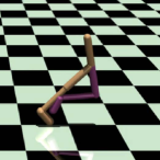
(b)

(c)

Figure 1: Snapshots of three robots.

We compare MADAC with two standard MARL algorithms as well as two safe MARL algorithms. HAPPO [8] is a state-of-the-art on-policy MARL method that extends the standard PPO algorithm [42] to multi-agent settings with an agent-by-agent sequential update scheme, facilitating convergence to a Nash equilibrium. HASAC [9] is a state-of-the-art off-policy MARL method with a similar structure to HAPPO but based on the maximum entropy framework of the SAC algorithm [39]. MACPO [17] is a state-of-the-art safe MARL method, which is the multi-agent extension of the standard CPO algorithm [28], using a trust-region approach for constrained policy updates. MAPPO-Lagrangian [17] is a state-of-the-art safe MARL method that extends the PPO-Lagrangian algorithm [43] to multi-agent scenarios, applying Lagrange multipliers for enforcing policy constraints.

The hyperparameters for HAPPO and HASAC are taken from the tuned configurations for standard (unconstrained) multi-agent MuJoCo environments in the open-source implementation provided by [8, 9]. The hyperparameters for MACPO and MAPPO-Lagrangian are taken from the tuned configurations in the open-source implementation provided by [17]. For each algorithm, we use the same set of hyperparameters across all environments, except for one adjustment with the Walker2D robot, where the learning rate of the Lagrange multipliers is increased for both MAPPO-Lagrangian and MADAC. Additionally, we do not terminate an episode when a constraint is violated, as this would blur the distinction between the algorithm’s reward-seeking capability and its safety-preserving capability. We expect the algorithm to discover safe behaviors on its own, which aligns with the setting in [41, 43]. An exception is made for MACPO in the Ant environments; without it, MACPO fails to learn, resulting in extremely negative episode returns.

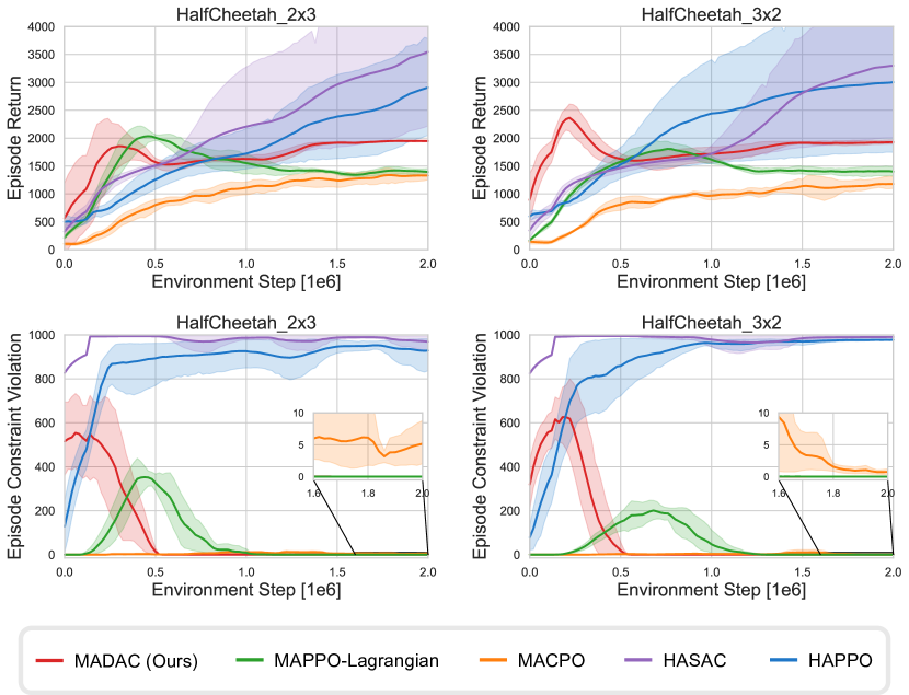
Figure 2: Training curves on HalfCheetah environments. While standard MARL baselines (HASAC and HAPPO) achieve higher rewards, they violate the constraints heavily. MADAC outperforms safe MARL baselines (MACPO and MAPPO-Lagrangian) by achieving significantly higher rewards, while maintaining equal or superior compliance with safety constraints.

We adopt two evaluation metrics in the training process: episode return and episode constraint violation. The training results of all algorithms for the six environments are shown in Figs. 2, 3, and 4. The solid lines correspond to the mean and the shaded regions correspond to 95% confidence interval over five seeds. The standard MARL algorithms, HAPPO and HASAC, violate constraints heavily in all environments, highlighting the need for properly designed safe MARL algorithms for safety-critical tasks. In general, among the safe MARL algorithms, our algorithm (MADAC) significantly outperforms MACPO and MAPPO-Lagrangian, achieving much higher rewards and fewer constraint violations. In the HalfCheetah environments, MAPPO-Lagrangian achieves similar safety-preserving performance to MADAC. However, in the more complex Walker2D and Ant environments, MAPPO-Lagrangian violates constraints more frequently than MADAC. MACPO performs the poorest among the three algorithms, as it struggles to learn a zero-violation policy even in the simplest HalfCheetah environments. A notable observation is that, in the HalfCheetah environments, MACPO shows fewer constraint violations during the early stages of training. This is because MADAC and MAPPO-Lagrangian, with their stronger reward-seeking capabilities, quickly learn to drive the robot faster (which violates the safety constraints heavily). As training progresses, both algorithms start to constrain the robot’s speed to meet the safety threshold. Another important observation is MADAC’s significant ability to achieve high rewards while maintaining safety. In the Ant environments, MADAC reaches returns comparable to HASAC but with significantly lower constraint violations. This demonstrates the effectiveness of MADAC’s underlying mechanism, multi-agent dual policy iteration, which seeks generalized Nash equilibria to maximize rewards while ensuring joint constraint satisfaction.

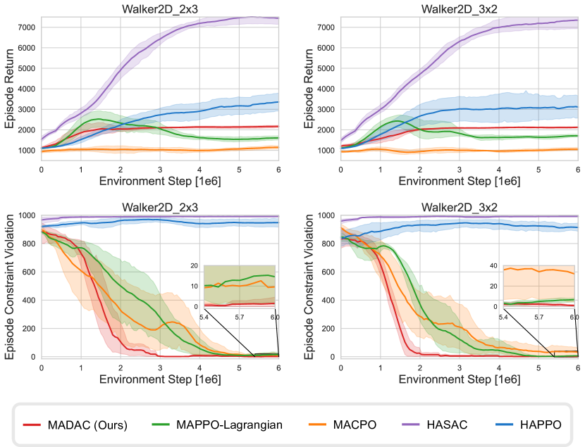
Figure 3: Training curves on Walker2D environments. While standard MARL baselines (HASAC and HAPPO) achieve higher rewards, they violate the constraints heavily. MADAC outperforms safe MARL baselines (MACPO and MAPPO-Lagrangian) by achieving significantly higher rewards, while maintaining equal or superior compliance with safety constraints.

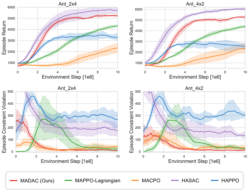
Figure 4: Training curves on Ant environments. Standard MARL baselines (HASAC and HAPPO) violate the constraints heavily. MADAC achieves rewards comparable to HASAC and substantially higher than HAPPO, while adhering to safety requirements. MADAC outperforms safe MARL baselines (MACPO and MAPPO-Lagrangian) by achieving significantly higher rewards, while maintaining equal or superior compliance with safety constraints.

6 Conclusion

In this paper, we presented a comprehensive framework for solving state-wise safe MARL problems, covering both theoretical analysis and algorithm design. We introduced a multi-agent approach for identifying controlled invariant sets that monotonically converges to a Nash equilibrium on safety value functions. We then embedded this method within a multi-agent dual policy iteration scheme that guarantees convergence to a generalized Nash equilibrium for state-wise constrained cooperative Markov games. Furthermore, we proposed the multi-agent dual actor-critic algorithm for effective deployment in complex high-dimensional systems. Experimental results on safety-critical MARL benchmarks demonstrate the effectiveness of our method.

References

- [1] Kaiqing Zhang, Zhuoran Yang, and Tamer Başar. Multi-agent reinforcement learning: A selective overview of theories and algorithms. Handbook of reinforcement learning and control, pages 321–384, 2021.
- [2] Shengbo Eben Li. Reinforcement Learning for Sequential Decision and Optimal Control. Springer Verlag, Singapore, 2023.
- [3] Ryan Lowe, Yi I Wu, Aviv Tamar, Jean Harb, OpenAI Pieter Abbeel, and Igor Mordatch. Multi-agent actor-critic for mixed cooperative-competitive environments. Advances in neural information processing systems, 30, 2017.
- [4] Ming Zhou, Ziyu Wan, Hanjing Wang, Muning Wen, Runzhe Wu, Ying Wen, Yaodong Yang, Yong Yu, Jun Wang, and Weinan Zhang. Malib: A parallel framework for population-based multi-agent reinforcement learning. Journal of Machine Learning Research, 24(150):1–12, 2023.
- [5] Tabish Rashid, Mikayel Samvelyan, Christian Schroeder De Witt, Gregory Farquhar, Jakob Foerster, and Shimon Whiteson. Monotonic value function factorisation for deep multi-agent reinforcement learning. Journal of Machine Learning Research, 21(178):1–51, 2020.
- [6] Dimitri Bertsekas. Multiagent reinforcement learning: Rollout and policy iteration. IEEE/CAA Journal of Automatica Sinica, 8(2):249–272, 2021.
- [7] Sushmita Bhattacharya, Siva Kailas, Sahil Badyal, Stephanie Gil, and Dimitri Bertsekas. Multiagent reinforcement learning: Rollout and policy iteration for pomdp with application to multi-robot problems. IEEE Transactions on Robotics, 2023.
- [8] Yifan Zhong, Jakub Grudzien Kuba, Xidong Feng, Siyi Hu, Jiaming Ji, and Yaodong Yang. Heterogeneous-agent reinforcement learning. Journal of Machine Learning Research, 25(1-67):1, 2024.
- [9] Jiarong Liu, Yifan Zhong, Siyi Hu, Haobo Fu, QIANG FU, Xiaojun Chang, and Yaodong Yang. Maximum entropy heterogeneous-agent reinforcement learning. In The Twelfth International Conference on Learning Representations, 2024.
- [10] Oriol Vinyals, Igor Babuschkin, Wojciech M Czarnecki, Michaël Mathieu, Andrew Dudzik, Junyoung Chung, David H Choi, Richard Powell, Timo Ewalds, Petko Georgiev, et al. Grandmaster level in starcraft ii using multi-agent reinforcement learning. nature, 575(7782):350–354, 2019.
- [11] Tianshu Chu, Jie Wang, Lara Codecà, and Zhaojian Li. Multi-agent deep reinforcement learning for large-scale traffic signal control. IEEE transactions on intelligent transportation systems, 21(3):1086–1095, 2019.
- [12] Chao Yu, Akash Velu, Eugene Vinitsky, Jiaxuan Gao, Yu Wang, Alexandre Bayen, and Yi Wu. The surprising effectiveness of ppo in cooperative multi-agent games. Advances in Neural Information Processing Systems, 35:24611–24624, 2022.
- [13] Guido Novati, Hugues Lascombes de Laroussilhe, and Petros Koumoutsakos. Automating turbulence modelling by multi-agent reinforcement learning. Nature Machine Intelligence, 3(1):87–96, 2021.
- [14] Weiye Zhao, Tairan He, Rui Chen, Tianhao Wei, and Changliu Liu. State-wise safe reinforcement learning: A survey. In International Joint Conference on Artificial Intelligence. IJCAI, 2023.
- [15] Daniel Melcer, Christopher Amato, and Stavros Tripakis. Shield decentralization for safe multi-agent reinforcement learning. Advances in Neural Information Processing Systems, 35:13367–13379, 2022.
- [16] Songtao Lu, Kaiqing Zhang, Tianyi Chen, Tamer Başar, and Lior Horesh. Decentralized policy gradient descent ascent for safe multi-agent reinforcement learning. In Proceedings of the AAAI conference on Artificial Intelligence, volume 35, pages 8767–8775, 2021.
- [17] Shangding Gu, Jakub Grudzien Kuba, Yuanpei Chen, Yali Du, Long Yang, Alois Knoll, and Yaodong Yang. Safe multi-agent reinforcement learning for multi-robot control. Artificial Intelligence, 319:103905, 2023.
- [18] Dongsheng Ding, Xiaohan Wei, Zhuoran Yang, Zhaoran Wang, and Mihailo Jovanovic. Provably efficient generalized lagrangian policy optimization for safe multi-agent reinforcement learning. In Learning for dynamics and control conference, pages 315–332. PMLR, 2023.
- [19] Donghao Ying, Yunkai Zhang, Yuhao Ding, Alec Koppel, and Javad Lavaei. Scalable primal-dual actor-critic method for safe multi-agent rl with general utilities. Advances in Neural Information Processing Systems, 36, 2024.
- [20] Youpeng Zhao, Yaodong Yang, Zhenbo Lu, Wengang Zhou, and Houqiang Li. Multi-agent first order constrained optimization in policy space. Advances in Neural Information Processing Systems, 36, 2024.
- [21] Eitan Altman. Constrained Markov Decision Processes: Stochastic Modeling. Routledge, 1999.
- [22] Kostas Margellos and John Lygeros. Hamilton–jacobi formulation for reach–avoid differential games. IEEE Transactions on Automatic Control, 56(8):1849–1861, 2011.
- [23] Dongjie Yu, Haitong Ma, Shengbo Li, and Jianyu Chen. Reachability constrained reinforcement learning. In International Conference on Machine Learning, pages 25636–25655. PMLR, 2022.
- [24] Zeyang Li, Chuxiong Hu, Yunan Wang, Yujie Yang, and Shengbo Eben Li. Safe reinforcement learning with dual robustness. IEEE Transactions on Pattern Analysis and Machine Intelligence, 2024.
- [25] Somil Bansal, Mo Chen, Sylvia Herbert, and Claire J Tomlin. Hamilton-Jacobi reachability: A brief overview and recent advances. In 2017 IEEE 56th Annual Conference on Decision and Control (CDC), pages 2242–2253. IEEE, 2017.
- [26] Sehoon Ha, Peng Xu, Zhenyu Tan, Sergey Levine, and Jie Tan. Learning to walk in the real world with minimal human effort. In Conference on Robot Learning, volume 155, pages 1110–1120. PMLR, 2021.
- [27] Yinlam Chow, Mohammad Ghavamzadeh, Lucas Janson, and Marco Pavone. Risk-constrained reinforcement learning with percentile risk criteria. Journal of Machine Learning Research, 18(1):6070–6120, 2017.
- [28] Joshua Achiam, David Held, Aviv Tamar, and Pieter Abbeel. Constrained policy optimization. In International Conference on Machine Learning, pages 22–31. PMLR, 2017.
- [29] Yiming Zhang, Quan Vuong, and Keith Ross. First order constrained optimization in policy space. Advances in Neural Information Processing Systems, 33:15338–15349, 2020.
- [30] Kai-Chieh Hsu, Haimin Hu, and Jaime F Fisac. The safety filter: A unified view of safety-critical control in autonomous systems. Annual Review of Control, Robotics, and Autonomous Systems, 7, 2023.
- [31] Aaron D Ames, Samuel Coogan, Magnus Egerstedt, Gennaro Notomista, Koushil Sreenath, and Paulo Tabuada. Control barrier functions: Theory and applications. In 2019 18th European control conference (ECC), pages 3420–3431. IEEE, 2019.
- [32] Changliu Liu and Masayoshi Tomizuka. Control in a safe set: Addressing safety in human-robot interactions. In Dynamic Systems and Control Conference, volume 46209, page V003T42A003. American Society of Mechanical Engineers, 2014.
- [33] Haitong Ma, Changliu Liu, Shengbo Eben Li, Sifa Zheng, and Jianyu Chen. Joint synthesis of safety certificate and safe control policy using constrained reinforcement learning. In Learning for Dynamics and Control Conference, pages 97–109. PMLR, 2022.
- [34] Justin Wang, Haimin Hu, Duy Phuong Nguyen, and Jaime Fernández Fisac. Magics: Adversarial rl with minimax actors guided by implicit critic stackelberg for convergent neural synthesis of robot safety. arXiv preprint arXiv:2409.13867, 2024.
- [35] Weiye Zhao, Rui Chen, Yifan Sun, Feihan Li, Tianhao Wei, and Changliu Liu. State-wise constrained policy optimization. Transactions on Machine Learning Research, 2024.
- [36] Jaime F Fisac, Neil F Lugovoy, Vicenç Rubies-Royo, Shromona Ghosh, and Claire J Tomlin. Bridging Hamilton-Jacobi safety analysis and reinforcement learning. In 2019 International Conference on Robotics and Automation (ICRA), pages 8550–8556. IEEE, 2019.
- [37] Jingqi Li, Donggun Lee, Somayeh Sojoudi, and Claire J Tomlin. Infinite-horizon reach-avoid zero-sum games via deep reinforcement learning. arXiv preprint arXiv:2203.10142, 2022.
- [38] Oswin So, Zachary Serlin, Makai Mann, Jake Gonzales, Kwesi Rutledge, Nicholas Roy, and Chuchu Fan. How to train your neural control barrier function: Learning safety filters for complex input-constrained systems. In 2024 IEEE International Conference on Robotics and Automation (ICRA), pages 11532–11539. IEEE, 2024.
- [39] Tuomas Haarnoja, Aurick Zhou, Pieter Abbeel, and Sergey Levine. Soft actor-critic: Off-policy maximum entropy deep reinforcement learning with a stochastic actor. In International conference on machine learning, pages 1861–1870. PMLR, 2018.
- [40] Emanuel Todorov, Tom Erez, and Yuval Tassa. Mujoco: A physics engine for model-based control. In 2012 IEEE/RSJ international conference on intelligent robots and systems, pages 5026–5033. IEEE, 2012.
- [41] Jiaming Ji, Borong Zhang, Jiayi Zhou, Xuehai Pan, Weidong Huang, Ruiyang Sun, Yiran Geng, Yifan Zhong, Josef Dai, and Yaodong Yang. Safety gymnasium: A unified safe reinforcement learning benchmark. Advances in Neural Information Processing Systems, 36, 2023.
- [42] John Schulman, Filip Wolski, Prafulla Dhariwal, Alec Radford, and Oleg Klimov. Proximal policy optimization algorithms. arXiv preprint arXiv:1707.06347, 2017.
- [43] Alex Ray, Joshua Achiam, and Dario Amodei. Benchmarking safe exploration in deep reinforcement learning. arXiv preprint arXiv:1910.01708, 7(1):2, 2019.