Threetangle in the XY-model class with a non-integrable field background

Abstract

The square root of the threetangle is calculated for the transverse XY-model with an integrability-breaking in-plane field component. To be in a regime of quasi-solvability of the convex roof, here we concentrate here on a 4-site model Hamiltonian. In general, the field and hence a mixing of the odd/even sectors, has a detrimental effect on the threetangle, as expected. Only in a particular spot of models with no or weak inhomogeneity $\gamma$ does a finite value of the tangle prevail in a broad maximum region of the field strength $h\approx 0.3\pm 0.1$. There, the threetangle is basically independent of the non-zero angle $\alpha$. This system could be experimentally used as a quasi-pure source of threetangled states or as an entanglement triggered switch depending on the experimental error in the field orientation.

Introduction – Entanglement is one of the main ingredients of modern quantum technology applications like quantum computationLadd et al. (2010); Gill et al. (2022); Orús et al. (2019); Ringbauer et al. (2022), quantum sensing and metrologyNarducci et al. (2022); Degen et al. (2017); Crawford et al. (2021); Wang et al. (2023); Aslam et al. (2023); Schnabel et al. (2010); Pezze et al. (2018); Polino et al. (2020), and quantum communicationGisin and Thew (2007); Luo et al. (2023a); Cozzolino et al. (2019); De Santis et al. (2024). However, finite temperature and experimental imperfections cast theoretically ideal models to the experimentally realistic realm of feasibility. Therefore it is extremely important to analyse the effect these imperfections have on this valuable resource. The focus here lies on multipartite entanglementHorodecki et al. (2009); Gühne and Tóth (2009); Eltschka and Siewert (2014a); Hein et al. (2004) for this resource. There are multiple ways to measure whether some multipartite entanglement might be in the system. The so-called Genuine Multipartite EntanglementTóth and Gühne (2005); Huber et al. (2010); Huber and Sengupta (2014); Milz et al. (2021), and the Generalized Multipartite NegativityVidal and Werner (2002); Jungnitsch et al. (2011) deliver useful information as far as a coarse grained classification of the entanglement content beyond bipartite entanglement is concerned. These are constructed from bipartite measures of entanglement as the Partial Transpose, and (linear) entropies of entanglement and are constructed to be zero for convex combinations of bipartite states. Another philosophy is applied in the (Generalized) Geometric EntanglementWei and Goldbart (2003); Sen et al. (2010); Das et al. (2016); Kondra et al. (2021); Blasone et al. (2008), where the distance to a certain class of states is detected. These can be but don’t necessarily need to be the separable states. For being more selective on the special type of entanglement, there exist measures for pure statesVerstraete et al. (2003); Osterloh and Siewert (2005); Osterloh (2016a), which are sufficiently relevant due to the vast amount of interesting features they accumulate in a single conceptOsterloh and Siewert (2005); D–oković and Osterloh (2009); Osterloh and Siewert (2010). To clearly distinguish from its bipartite cousin, we call it genuine multipartite SL-entanglement. We preserve the term tangle as an umbrella term for multipartite SL-entanglement measures. The drawback of these SL-invariant measures is that they have a non-linearity of $2n$ in the wave function entries. This lifts their convex-roof extension from the integrable regime of the concurrence with second degree non-linearity to being a highly non-trivial taskGurvits (2003). A degree two measure of SL-entanglement still exist for all even number of qubits that is integrable with respect to obtaining their convex-roof but it only covers the generalized GHZ stateOsterloh and Schützhold (2017). Even though it is futile to look for an exact solution of the convex roof due to the NP-hardness of the problemGurvits (2003) in general, it is extremely useful to study the behavior of optimal decompositions in simple cases, in order to elaborate an approximative scheme of structural similarity to perturbation theory along the lines of  Osterloh (2016b, a). We compare our results to a lower bound to the one parameter family of GHZ-symmetric statesEltschka and Siewert (2014b, a). Obtaining new such lower bounds is cumbersome since it requires multiple parameters to be optimized over.

We here study a quantity that singles out GHZ-type of SL-entanglement, namely the threetangleCoffman et al. (2000), and analyze its dependence on an integrability breaking field in the class of transverse XY models. We utilize an upper bound approach in that we construct quasi-optimal decompositions of the density matrix in consideration, but argue that the result is the exact convex roof because the maximal amount of states in this case is limited by $4$, and based on the state-lockingOsterloh (2016a) of the zero-polytope in optimal decompositions.

Model Hamiltonian – We deal with the Hamiltonian

$$H = -\sum_{j=1}^{L}\left[\frac{1+\gamma}{2}\sigma_{j}^{x}\sigma_{j+1}^{x}+\frac{1-\gamma}{2}\sigma_{j}^{y}\sigma_{j+1}^{y}\right.$$ (1)

$$\quad\left.+h(\sigma_{j}^{z}\cos{\alpha}+\sigma_{j}^{x}\sin{\alpha})\right]\;,$$

where $L$ is the number of sites, $\gamma$ is the isotropy parameter, $h$ is the magnetic field, and $\sigma^{.}_{j}$ are the Pauli matrices. For the angle $\alpha=0$ this is the integrable XY model in transverse fieldMcCoy et al. (1971). A non-zero angle $\alpha$ leads to a ${\sf Z\kern-4.40002ptZ}_{2}$ symmetry breaking and thus the odd and even sectors, which before were conserved, become intertwined. A non-zero $\alpha$ can be either due to experimental imperfections or it may be introduced willingly to destroy the integrability. Of course, it is interesting how various correlations behave and in particular would it be intriguing to see how entanglement quantifiers behave in presence of a non-zero angle. Here, we are interested in quantifiers, which detect the genuine SL-invariant part of the entanglement content; among them, most prominently, the concurrenceWootters (1998) and the threetangleCoffman et al. (2000) $\tau_{3}$ (see Appendix B) which will be detected by $\sqrt{\tau_{3}}$Viehmann et al. (2012). For the purposes of this work, we deal only with the four site model as it has the advantage of exact predictive power where the entanglement vanishes. We draw a comparison with the lower bound from GHZ-symmetric states.

For a general $\alpha\neq 0$ the eigenstates of the Hamiltonian (1) are superpositions of eigenstates of both parity sectors. Only the two groundstates will have an essential participation and the ground state will be approximately given by a superposition $|\psi_{\rm GS}\rangle(p):=\sqrt{p}|\psi_{o}\rangle+\sqrt{1-p}|\psi_{e}\rangle$, $p\in\{0,1\}$, and $\partial_{p}H=0$, $\partial_{p}^{2}H>0$. However, for the four site model the ground state is found by means of an exact diagonalisation.

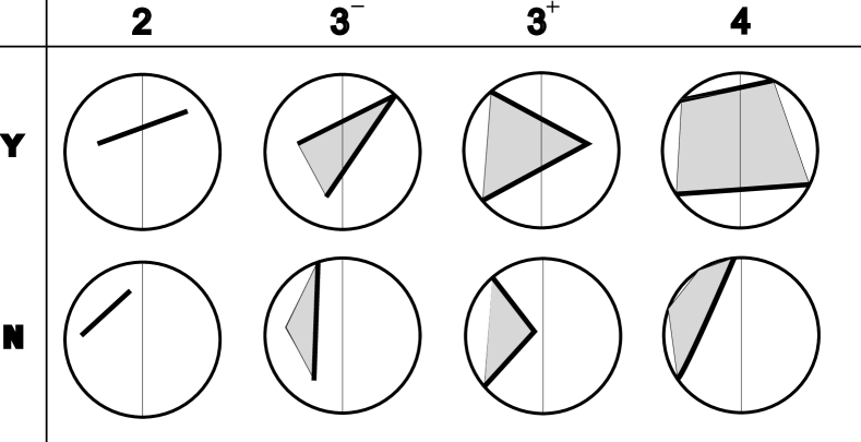
Figure 1: Complete classification of polytopes for real eigenstates of the density matrix in the real $x-z$-plane. Shown are typical examples for the model Hamiltonian. Every rotation of the zero polytope about the $y$-axis may lead to another classification. For the rightmost two columns, each of the distributions of $n$ pure states is possible with $n\in\{0,1,2,3\}$ for both orientations. Here only the evenly distributed cases are depicted.

Given that the wavefunction for the groundstates is strictly real, the solutions for the zero-polytope Osterloh et al. (2008); Osterloh (2016a) are grouped in complex conjugated pairs. There are eight different types of polytopes of particular relevance here; for each of them there is one intersecting the $z$-axis of the Bloch sphere (Y) and one that does not (N). They are shown in Fig. 1 in the ($x-z$) plane so that each complex solution $z$ and $z^{*}$ are projected onto the same point. Therefore, each vertex in the inner part of this projected Bloch sphere represents two complex conjugated solutions. Each bold line marks a side of the polytope, which is visible from a state $\rho$ the $z$-axis and that therefore can be part of an optimal decompositionOsterloh (2016a); Neveling (2019) for it. For a point $\vec{b}$ inside this projection of the Bloch sphere being member of an optimal decomposition for a density matrix $\rho_{0}$ lying on the $z$-axis at $\vec{r}_{0}$ of the Bloch sphere, it is clear that the remaining states from the zero-polytope that completes the optimal decomposition will correspond to a point $\vec{z}$ on the line $\vec{b}-\vec{r}_{0}$. Due to the reality of the ground state, we further have that every element $\vec{b}$ in the optimal decomposition has its complex conjugated solution $\vec{b}^{*}$ yielding the same value for the tangle. So, without loss of generality, we have that $\vec{b}_{0}=(\vec{b}+\vec{b}^{*})/2$ is real and corresponds precisely to the real point within the Bloch sphere projection. Combined, both arguments lead to the real point $\vec{z}_{0}$ that lies closest on the connecting line $\vec{b}_{0}-\vec{r}_{0}$.

Every decomposition is classified by two numbers, $n_{0}$ and $n_{e}$, by $(n_{0},n_{e})$. Whereas $n_{0}$ is the number of pure states taken from the zero-polytope, $n_{e}$ is the corresponding number of entangled pure states in the decomposition. Its tangle is given by convex combination of the corresponding density matrix: $\rho_{0}=\sum_{i=1}^{n_{0}}m_{i}|Z_{\nu_{i}}\rangle\langle Z_{\nu_{i}}|+\sum_{\varepsilon=1}^{n_{e}}M_{\varepsilon}|T_{\varepsilon}\rangle\langle T_{\varepsilon}|$ $\Rightarrow\tau=M_{\varepsilon}\tau[T_{\varepsilon}]$, where $T_{\varepsilon}$ are the entangled states in the decomposition and $\tau$ is the tangle. Any decomposition that reaches the minimum for the mixed state $\rho_{0}$ is an optimal decomposition. The main working assumption is that optimal decomposition must continuously vary in the available parameters. The probability $p$ connecting both eigenstates of the density matrix is the only parameter here.

Our approach is to first look at the minimum solution with one single pure state out of the zero-polytope, i.e. optimal $(n_{0},1)$-solutions. This gives some insight of how these optimal decompositions behave. We make use of the behavior known for optimal decompositionsOsterloh and Siewert (2005); Eltschka et al. (2008); Osterloh (2016b, a); Viehmann et al. (2012). In the next step we tried to look whether $(n_{0},2)$-decompositions optimize the result, admitting the pure state to split into two, maintaining the connecting axis the optimal $(n_{0},1)$ decomposition had with the density matrix.
The first non-trivial result is that, what we call ”brachiating states”, are optimal $(n_{0},1)$-decomposition. For this, we have analysed polytopes of the type $3^{+}Y/N$ as the main contributors for this model (see Fig. 1). We list some general requirements on optimal decompositions in Appendix A.

Brachiating states – Before turning to the more relevant case of two-dimensional zero-polytopes, we briefly want to highlight one-dimension polytope with two equally degenerate solutions. This is the integrable situation for the convex roof as for the concurrence: here every $(n,1)$ decomposition is optimal, giving the same result for the tangle. This case has been analyzed in Ref. Regula and Adesso (2016a, b) and it could be observed also in this work.
The symmetric case for type $4Y$ with two values $p_{i}$ with opposing phases is the only one occurring in the transverse models. The exact convex roof is obtained from a standard procedure, with corresponding pure states located precisely in the poles of the sphere as for the symmetric GHZ-W mixtureLohmayer et al. (2006). Interesting is the asymmetric case for which a case study is shown in Ref. C.

Polytopes of type $2N$ occured for the XX model with non-orthogonal field. In these cases we have run an extra analysis of general $(2,1)$ decompositions for optimality due to an initial error in the algorithm. Both $(2,1)$ decompositions have been analyzed with the states corresponding to the real parts $z_{0;i}$, $i=1,2$. It is found that the respective minimum is either in the middle or at the end points, hence for $(1,1)$ decompositions. The minimal tangle was found in the center $z_{0;i}$ that lied closer to the state in consideration. We want to stress that a minimum elsewhere on the Bloch sphere would mean that a state with complex part would be singled out that forms an optimal $(2,1)$ decomposition; i.e., the same would be true for the corresponding complex conjugated images of these states. This would enlarge the optimal decomposition to $(2,2)$ type. This has never been found optimal in the model of consideration.

Three dimensional polytopes of type $3$ – Both zero-polytopes $3^{+}w$ for $w=Y,N$, among others, do occur for certain regions of the parameters of (1) and give interesting insights in the behavior of optimal decompositions. First we discuss the $3^{+}N$ class which does not cross the central axis of the Bloch sphere. It is clear that the corresponding tangle will be non-zero outside the zero-polytope, hence for the whole polar axis of the Bloch sphere. The two sets $3^{\pm}Y/N$ are equivalent in what the optimal decomposition is concerned. We describe the analysis of $3^{+}Y$ in more detail in Appendix D, but give a summary of the findings here.

The relatively optimal decomposition of type $(n_{0},1)$ can be obtained in two steps which is indicated in the right Bloch sphere in Fig. 2: identifying the two points $p^{+}_{\rm low}$ and $p^{-}_{\rm high}$ where the z-axis leaves the zero polytope and the both points $p^{+}_{\rm high}$ and $p^{-}_{\rm low}$ where the z-axis leaves the respective $(3,1)$ polytopes with singled out states $|N_{\pm}\rangle$. These polytopes are attached to all the sides of the zero polytopes. The two lines $\overline{p^{\pm}_{\rm low}p^{\pm}_{\rm high}}$ where the tangle as a convex combination grows linearlyLohmayer et al. (2006); Osterloh et al. (2008); Osterloh (2016a) are highlighted in bold. Beyond these linear behaviors the tangle behaves strictly convex as only a single zero state ($|Z_{3}\rangle$ or $|Z_{4}\rangle$) is left for optimal $(1,1)$ decompositions as indicated by green lines.

In the case of $3^{+}N$ polytopes, we have to analyse both $(1,1)$ decompositions with $|Z_{3}\rangle$ and $|Z_{4}\rangle$ in comparison with the $(2,1)$-decomposition including the both states $|Z_{1/2}\rangle$. A case study is shown in Fig. 7. Here we focus on the two pure states $|N_{\pm}\rangle$ corresponding to the two facets visible from the $\psi_{0}$-$\psi_{1}$ axis. Due to the reality of the wavefunction $|N_{\pm}\rangle$ come to lie at phases $\phi=0$ (the right meridian drawn) or $\phi=\pi$ on the Bloch sphere.

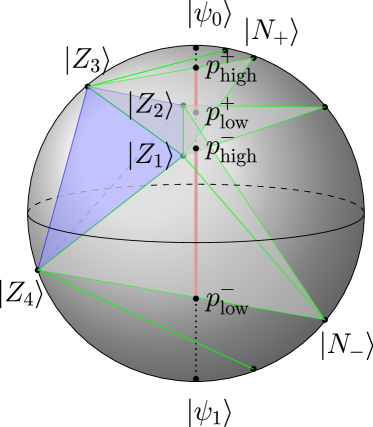
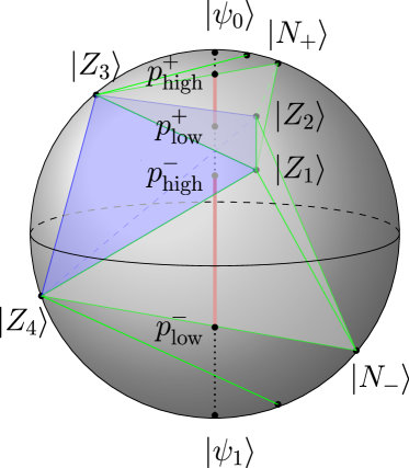
Figure 2: Polytopes of type $3^{+}N$ (left figure) and $3^{+}Y$ (right figure). Shown is that to the zero polytope (blue) a single pure state on the Bloch sphere is added corresponding to each of its zero-facets, respectively. They give rise to another simplex (grey triangular tetrahedra) lying on top of the corresponding 2-dimensional simplices of the zero-polytope. This is a general feature for every simplex on the surface of zero-polytopes. Optimal decompostions, here indicated by green lines, brachiate through this structure of polytopes.

It is seen that the minimum of these three curves is not convex. Result are single pure states, $|N_{\pm}\rangle$ in a $(3,1)$-decomposition. This is demonstrated by the coinciding $p$-values of either state. In principle, it could be that different pure states were responsible for both convexification points. This would correspond to $5$ pure states in an optimal decomposition and their convex set forms the polytope. Though, always four out of the five states can be chosen as optimal decomposition. Included is a search for optimality of $2$ entangled states in the decomposition. The values of the tangle are shown exemplarily for the green curve. A more detailed analysis of these deviations into both two dimensional $(2;2)$- or $(1;2)$-decompositions was never optimal for this Hamiltonian. However, it must be stated, that this is done by inspection and a strict proof of this statement is missing. In general, we cannot exclude that these 2-dimensional decompositions are optimal nowhere in the Bloch sphere.

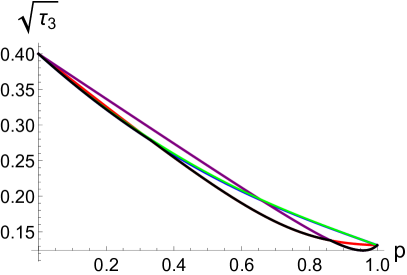
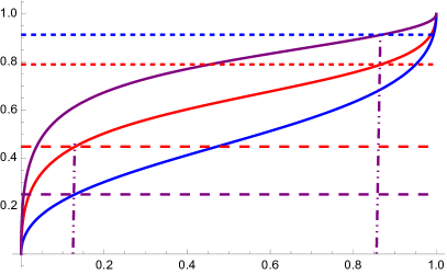
Figure 3: $\sqrt{\tau_{3}}$ is shown in the left panel for the $(2,1)$ (red) and $(1,1)$ (blue and purple) decompositions for a zero-polytope of classes $3^{+}N$. The minimum is given by the black curve underneath. Convexifications are obviously needed. It leads to a single 3D simplex on top of each visible sides of the zero-polytope as a basis. This is shown in the right panel where $p_{0}$ of $\rho[p_{0}]$ is plotted as a function of the $p$-value of the corresponding pure state as tip of that tetrahedron.

Summarizing, a single pure state on the Bloch sphere is added to the zero polytope (blue) corresponding to each of its zero-facets. Together with the three pure states of the zero-polytope lying on top of the corresponding 2-dimensional simplices of the zero-polytope, they form polytopes outside of the zero polytope, like the two polytopes highlighted in grey - Fig. 2. We want to stress that this is a more general feature for every simplex on the surface of zero-polytopes.

The optimal decompostions, here indicated by green lines, brachiate through this structure of tetrahedra with an additional pure state at $\phi=0$. Following Fig. 2 the optimal $(1,1)$-decomposition starts with the lowest pure state $|Z_{4}\rangle$ of the zero polytope and the second pure state brachiates through until it reaches $\vec{n}_{-}\mathrel{\widehat{=}}|N_{-}\rangle$ with value $p_{\rm low}^{-}$ in $\rho(p_{\rm low}^{-})$. This state gets fixed next in the lower grey pyramid and the state brachiates on the bisecting line in a $(3,1)$-decomposition until $\rho(p_{\rm high}^{-})$ where it will be located in the center of the both states $|Z_{1}\rangle$ and $|Z_{2}\rangle$. Next these two states of the zero polytope get locked with a variable pure state on the Bloch sphere in a $(2,1)$-decomposition until it reaches $|N_{+}\rangle$ and $\rho(p_{\rm low}^{+})$. Being this new pure state $|N_{+}\rangle$ the fixed point, the variable mixed state again brachiates along the bisecting line until it reaches the state $|Z_{3}\rangle$ in $(3,1)$-decompositions. Afterwards the optimal decomposition swings up in a $(1,1)$-decomposition until the upper pole of the Bloch-sphere is reached. This brachiating behavior of optimal decompositions was observed in Ref. Neveling (2019). It gives a scheme how optimal decompositions behave in general for the threetangle and in general for arbitrary tangles iff the density matrix has rank two.

Analysis for non-zero alpha – For the non-transverse XY-model, we observe that its largest eigenvalues for three-site density matrices is very close to one such that $(1;1)$- and $(2;1)$-decompositions are optimal. We nowhere observed that the value for $p$ of the model considered was inside an convexified area. The results are shown in Fig. 4. For larger values of $\gamma$ the value for $\sqrt{\tau_{3}}$ quickly decays for $\alpha\neq 0$ and will be discussed in a forthcoming paper. $\alpha$ is show in multiples of $\pi$ from $\alpha=0$ to $\alpha=\pi/2$. We show curves for $\gamma=0.0$ and $0.1$ in Fig. 4. $\sqrt{\tau_{3}}$ is algebraically decreasing with the angle $\alpha$. For the XX model there is a pronounced peak at finite $\alpha$ with a maximum roughly at $h=0.5$ and $\alpha=0.03$; while $\tau_{3}$ decays algebraically in this maximum to a relative minimal value at $\alpha=\pi/2$, $\sqrt{\tau_{3}}$ proves to be essentially unaffected by the angle at an intermediate value of $h=0.3$ with reasonably high values of $\sqrt{\tau_{3}}\approx 0.1$. The independence of the latter on the alignment of the field is observed also for small values of $\gamma$ up to $\gamma=0.3$ with a value of $\sqrt{\tau_{3}}$ is still about $0.05$. For models away from the symmetric XX model, we immediately see the typical maximum for $\sqrt{\tau_{3}}$ at vanishing angle $\alpha$. Away from this maximum $\sqrt{\tau_{3}}$ rapidly decays about an order of magnitude when the angle is about $\alpha=0.03\,\pi$. This could be used to trigger the entanglement in a switch like situation having as a knob the orientation of the magnetic field. Likewise the independence of the entanglement of the field orientation might be used in environments where the orientation of the field is much less accurately controllable than its strength.

We do not show curves for higher values of $\gamma$ and refer to a forthcoming publicationOsterloh . However, the only behavior which survives there is the quick decay to about one order of magnitude from the maximum value for vanishing $\alpha$Osterloh . There is no reasonably large $\tau_{3}$ any longer. The region of strictly absent $\tau_{3}$ is slightly enlarged from $h=0.1$ at $\gamma=0.1$ to $h=0.3$ for $\gamma=0.5$ for being reduced again for larger values of $\gamma$. They could be still used as sensitive entanglement switch with the orientation of the magnetic field.

We compare the results with the lower bound from GHZ-symmetric statesEltschka and Siewert (2012a); Siewert and Eltschka (2012) in Fig. 5. For higher values of $\gamma$ and in the limit of $\alpha\to\pi/2$ it approximates our results well with more pronounced under-estimations for small values of $\alpha$ where our result turns to a provably exact valueLohmayer et al. (2006); Osterloh et al. (2008). Inaccuracies in the algorithm are mainly due to $(1,2)$ and $(2,2)$ decompositions, which would result in invisible changes on the scale of the tangle. These under-estimations of the lower bound have been first noticed and outlined in Ref. Osterloh (2016a). For smaller values of $\gamma$ and in particular for the XX-model, it fails to predict the finite value of $\sqrt{\tau_{3}}$ also for higher values of $\alpha$ which could gain experimental relevance. There the model is apparently sufficiently off the GHZ-symmetric case.

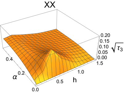
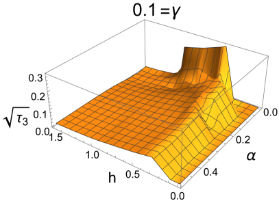
Figure 4: Entanglement detected by $\sqrt{\tau_{3}}$ for the reduced density matrix interpolating between both of its eigenstates as a function of the deviation angle $\alpha$ of the magnetic field. We show curves for $\gamma=0.0$ and $0.1$. The tangle $\sqrt{\tau_{3}}$ is algebraically decreasing with the angle $\alpha$. At about $h=0.3$ lies a broad maximum of $\sqrt{\tau_{3}}$ which is not notably changed in varying $\alpha$. From $\gamma=0.5$ (not shown) this effect is absent and the tangle in the system is destroyed immediately. Therefore the field to be transversally aligned is a hot-spot which does not support non-transversality of the field.

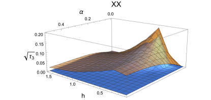
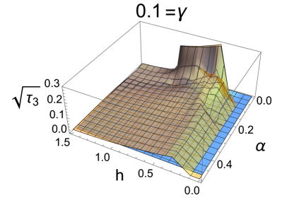
Figure 5: Comparison of the result found here (transparent orange) with the lower bound from GHZ-symmetric states (blue). A reasonably large difference, in particular for values which are close to the isotropic XX model, is observed as already noticed in Ref. Osterloh (2016a).

Conclusions – The transverse XY models have been studied theoretically in a symmetry breaking field of given strength but with a deviation angle $\alpha$ from transversality. The model has been analysed for four sites, which provides a standard situation where the density matrix on three sites is strictly of rank 2 and therefore is accessible to a quasi-exact treatment. The measure of entanglement is the genuine multipartite SL-entanglement, measured here by the square root of the threetangle.

The general behavior is a detrimental effect whenever field inclinations are observed. Only the model with small anisotropy parameter $\gamma$ shows a remarkable resistance to this symmetry breaking field. Wheras the isotropic transverse model is disentangled in the threetangle it develops a steep maximum or pike at about $h=0.5$ and $\sqrt{\tau_{3}}\approx 0.2$. It tends to be independent of $\alpha$ for basically all investigated values of $h$ but with a maximum observed about $h=0.3$. In a reasonable range about this value of $h$, we observe fixed $\sqrt{\tau_{3}}\approx 0.1$. For a inhomogeneity of $\gamma=0.5$ and larger, this effect vanishes. Hence, from an initially disentangled state the symmetry breaking and mixing of the two parity sectors of the ${\sf Z\kern-4.40002ptZ}_{2}$ symmetric model creates the entanglement for this case. This is important from an experimental point of view because one can choose the parameter region properly and generates an output state with a reasonable value of $\sqrt{\tau_{3}}\approx 0.1$ which also is observed to be quasi-pure. This is not observed using the lower bound. The output state could then be fed into entanglement purification/distillation protocols. This would guarantee a source where this class of entanglement is necessary. The system could also be used as a sensitive entanglement switch around the maxima of the tangle at $\alpha=0$. The tangle could be checked experimentally either by full state tomography as a proof of principle but also by every measure of multipartite entanglementZhang and Nori (2023); Cao et al. (2024); Malla et al. (2023); Wu et al. (2024); Li et al. (2024) or by witnessesGühne and Tóth (2009); Iglói and Tóth (2023) once the nature of entanglement having been established. Also the detection via Machine Learning or Neural Networks, as suggested in Refs. Luo et al. (2023b); Gulati et al. (2024) is a possibility.

As byproduct a behavior of optimal decompositions for general SL-tangles could be singled out: simplified they are brachiating among states, which are visible states of the zero-polytope on the one side and specific entangled states on the Bloch sphere on the opposite side. These states must be found by a convexification protocol. The peculiar behavior of optimal decompositions could be harnessed for many important tasks as looking towards an order dependent deviation as perturbation theory. For this task, it would be of utmost importance to develop lower bounds along the lines of Ref. Eltschka and Siewert (2012b, 2014b).

Finally, the quasi pureness of the eigenstates apparently survives switching on the integrability breaking field. This could be used for calculating the threetangle for these models along the lines of Ref. Osterloh (2016b).

Acknowledgements – We thank TII and in particular L. Amico for supporting this research.

Here is a collection of results that are used for the calculations or supporting evidence the for results. We start with remarks on optimal decompositions and parametrization of the states in the rank-two situation.

Appendix A General properties of optimal decompositions for real states of rank two

In Refs. Carathéodory (1911); Uhlmann (1998) it is shown that for the number of pure states contained in any optimal decomposition, $n_{\rm opt}$, we have ${\rm rank}[\rho]\leq n_{\rm opt}\leq({\rm rank}[\rho])^{2}$. Here that means that it is sufficient to look for up to $4$ such pure states which form in general three dimensional simplices. We want to emphasize that more than the maximal $4$ states may be in an optimal decomposition; in this case every $4$ states out of that decomposition are optimal as well and the optimal decomposition is given by the convex polytope made out of these points. The tangle will behave linear in these optimal polytopes.
If the density matrix is made of real entries only, as is the case for the ground state of a Hamiltonian which is non-degenerate, then every tangle $\tau$ has the property that $\tau(z)\equiv\tau(z^{*})$ where $|\psi\rangle\propto|\psi_{1}\rangle+z|\psi_{2}\rangle$ is a representation that corresponds to a vector onto the Bloch-sphere with the parametrizationOsterloh (2016a)

$$z\mathrel{\widehat{=}}\vec{n}=\left(\begin{array}[]{c}x\\ y\\ z\end{array}\right)=\left(\begin{array}[]{c}2\sqrt{p(1-p)}\cos\phi\\ 2\sqrt{p(1-p)}\sin\phi\\ 2p-1\end{array}\right)$$ (2)

where $|\psi_{i}\rangle$ are the two anti-podes on the z-axis. Real superpositions lie in the $(x-z)$-plane. If two vectors corresponding to $z_{i}$, $i=0,1$ give an optimal decomposition with $z_{0}$ being on an external edge of the zero-polytope, so do $z_{i}^{*}$. Therefore, the union of pure decomposition states is also an optimal decomposition. Within the same reasoning we can as well take the real values $z_{i,r}$ as reference values for searches after optimal decompositions. This leads to

$$z_{i,r}\mathrel{\widehat{=}}\vec{n}_{i}=\left(\begin{array}[]{c}2\sqrt{p_{i}(1-p_{i})}\cos\phi_{i}\\ 0\\ 2p_{i}-1\end{array}\right)$$ (3)

where it will be of particular interest a) where the line $\overline{\vec{n}_{0}\vec{n}_{1}}$ cuts the $z$-axis, b) which are the weights of the corresponding entangled state(s), and c) where it crosses the Bloch sphere, that is the corresponding pure states. Whereas the answer to a) is given by the probability

$$P=\frac{p_{0}\sqrt{p_{1}(1-p_{1})}\cos\phi_{1}+p_{1}\sqrt{p_{0}(1-p_{0})}\cos\phi_{0}}{p_{0}\sqrt{p_{0}(1-p_{0})}\cos\phi_{0}+p_{1}\sqrt{p_{1}(1-p_{1})}\cos\phi_{1}}$$ (4)

such that the point is located in $\vec{n}_{P}=(2P-1)\vec{e}_{z}$, the answer to b) is given by

$$\lambda=\frac{\mu_{1}}{\mu_{0}}=\frac{\sqrt{p_{0}(1-p_{0})}\cos\phi_{0}}{\sqrt{p_{1}(1-p_{1})}\cos\phi_{1}}$$ (5)

and for the mainly interesting case of $\cos\phi_{1}=0$ and $p$ being the probability in the density matrix in consideration we obtain as a solution to c)

$$P_{\pm}=p_{0}+\frac{p-p_{0}}{2}\frac{(p-p_{0})(1-2p_{0})+2p_{0}(1-p_{0})\cos^{2}\phi_{0}\pm\sqrt{(p_{0}-p)^{2}+4pp_{0}(1-p_{0})(1-p)\cos^{2}\phi_{0}})}{(p-p_{0})^{2}+p_{0}(1-p_{0})\cos^{2}\phi_{0}}$$ (6)

We refer to the Appendix A for a collection of formulas used.

Since every sub-partition of an optimal decomposition is itself optimal it gives a convex composition of the tangle values of the respective pure states. This strictly linear behavior inside all the simplices of an optimal decomposition also indirectly tells about whether there will be some more states in a decomposition for being optimal: the continuation of the respective decomposition type leads to a convex behavior in the tangle value. This holds in particular if the corresponding optimal polytope changes dimension, here, this means to dimensionality at most three. It must be noted that here for $(n_{0},n_{f})$-decompositions with $n_{f}>1$ the weight on the $n_{f}$ states necessarily increases as the projection on the $(x-z)$-plane moves closer to the density matrix in consideration. This must be overcompensated by a decreasing of the tangle of the corresponding pure states on the Bloch sphere. Therefore, a relative maximum would be favorable for this to happen; however, far away from the states $|Z_{i}\rangle$ the tangle behaves smoothly and in particular, there are no ripples seen. The presence of such ripples would indicate a much higher degree of the respective polynomial which however would be reflected mainly in more zeroes. In particular this also means that it must not be looked after a vertical splitting of the pure state in the $(2,1)$-decompositions here since the result would be a three-dimensional tetrahedron which cuts the polar line of the Bloch sphere in an interval of non-zero length. This indicates a linear slope of the tangle. But every linear connection line lies above a strictly convex behavior of the tangle. Hence it cannot be optimal in this case.

sectionCollection of useful formulae

We here consider the weight laid on a state to ensure that the convex combination is in $2p-1$ on the $z$-axis, where $p$ is the weight of the density matrix.

A.1 $(1,1)$-decompositions

Here, we have a $(1,1)$-decomposition of a pure state at z-coordinate $2p_{1}-1$ where $p_{1}$ corresponds to its probability of the two states $|\psi_{i}\rangle$; $i\in\{N,S\}$. We find

$$l_{1}(p_{1},p) = 2\sqrt{(p-p_{1})^{2}+p_{1}(p_{1}-1)}$$ (7)

$$l_{2}(p_{1},p) = \frac{4p(1-p)}{l_{1}(p_{1},p)}$$ (8)

$$m_{2}(p_{1},p) = \frac{l_{1}(p_{1},p)}{l_{1}(p_{1},p)+l_{2}(p_{1},p)}$$ (9)

$$p_{2}(p_{1},p) = \frac{4p^{2}(1-p_{1})}{l_{1}(p_{1},p)^{2}}=(1-p_{1})\frac{p}{1-p}\cdot\frac{l_{2}(p_{1},p)}{l_{1}(p_{1},p)}$$ (10)

$$p(p1,p2) = p_{1}+\frac{(p_{2}-p_{1})\sqrt{p_{1}(1-p_{1})}}{\sqrt{p_{1}(1-p_{1})}+\sqrt{p_{2}(1-p_{2})}}$$ (11)

Next we want to examine whether for a given $(1,1)$ decomposition with $p_{1}$, $p_{2}$, and $p$ it is convenient to split the pure state in two to give a $(1,2)$ decomposition. It can be seen that the ratios $x_{1}/(2|p_{1}-p|)=x_{2}/(2|p_{2}-p|)=x^{\prime}_{2}/(2|p^{\prime}_{2}-p|)$ with $y^{\prime}_{2}=\pm\sqrt{4p^{\prime}_{2}(1-p^{\prime}_{2})-{x^{\prime}}_{2}^{2}}$. For the new $p^{\prime}_{2}$ of this new state at phase $\phi_{2}$ the calculation gives

$$p^{\prime}_{2}(p_{1},p;\phi_{2})=p_{1}+(p-p_{1})\frac{2p_{1}(1-p_{1})-(p-p_{1})(2p_{1}-1)\cos^{2}\phi_{2}+\cos\phi_{2}\sqrt{4p(1-p)p_{1}(1-p_{1})+(p-p_{1})^{2}\cos^{2}\phi_{2}}}{2(p_{1}(1-p_{1})+(p-p_{1})^{2}\cos^{2}\phi_{2})}$$ (12)

A.2 $(2,2)$-decompositions

In the following we will assume that both are corresponding to a superposition of two states at $p_{i}$ and angles $\pm\phi_{i}$, $i\in\{1,2\}$, so that both states come to lie inside the Bloch sphere.

We find

$$m_{2}(p_{1},\phi_{1};p_{2},\phi_{2}) = \frac{\sqrt{p_{1}(1-p_{1})\cos^{2}(\phi_{1})}}{\sqrt{p_{1}(1-p_{1})\cos^{2}(\phi_{1})}+\sqrt{p_{2}(1-p_{2})\cos^{2}(\phi_{2})}}$$ (13)

$$= \frac{l_{1}(p_{1},\phi_{1};p_{2},\phi_{2};p)}{l_{1}(p_{1},\phi_{1};p_{2},\phi_{2};p)+l_{2}(p_{1},\phi_{1};p_{2},\phi_{2};p)}$$ (14)

$$m_{1}(p_{1},\phi_{1};p_{2},\phi_{2}) = 1-m_{2}(p_{1},\phi_{1};p_{2},\phi_{2})$$ (15)

$$p(p_{1},\phi_{1};p_{2},\phi_{2}) = p_{1}+(p_{2}-p_{1})\frac{\sqrt{p_{1}(1-p_{1})\cos^{2}(\phi_{1})}}{\sqrt{p_{1}(1-p_{1})\cos^{2}(\phi_{1})}+\sqrt{p_{2}(1-p_{2})\cos^{2}(\phi_{2})}}$$ (16)

$$= \frac{p_{2}\sqrt{p_{1}(1-p_{1})\cos^{2}(\phi_{1})}+p_{1}\sqrt{p_{2}(1-p_{2})\cos^{2}(\phi_{2})}}{\sqrt{p_{1}(1-p_{1})\cos^{2}(\phi_{1})}+\sqrt{p_{2}(1-p_{2})\cos^{2}(\phi_{2})}}$$ (17)

$$= p_{1}m_{1}(p_{1},\phi_{1};p_{2},\phi_{2})+p_{2}m_{2}(p_{1},\phi_{1};p_{2},\phi_{2})$$ (18)

$$l_{1}(p_{1},\phi_{1};p_{2},\phi_{2};p) = 2\sqrt{(p_{1}-p)^{2}+p_{1}(1-p_{1})\cos^{2}\phi_{1}}$$ (19)

$$l_{2}(p_{1},\phi_{1};p_{2},\phi_{2};p) = 2\sqrt{(p_{2}-p)^{2}+p_{2}(1-p_{2})\cos^{2}\phi_{2}}$$ (20)

From this it is seen that the weights of the states are symmetric under exchanging $p_{i}\to 1-p_{i}$ separately for $i\in\{1,2\}$.

Usually, only one or two pure states are known together with the parameter $p$ of the mixed state on the $z$-axis. It is then slightly more tedious calculating the respective variables though one could in principle obtain them via the theorem of implicit functions. We have not chosen this part and preferred to solve the linear algebraic geometric equations instead. The result for setting $\phi_{2}=0$ is

$$p_{2}(p_{1},\phi_{1};p)=p_{1}+(p-p_{1})\frac{(p_{1}-p)(2p_{1}-1)+2p_{1}(1-p_{1})\cos^{2}\phi_{1}+\sqrt{(p_{1}-p)^{2}+4p(1-p)p_{1}(1-p_{1})\cos^{2}\phi_{1}}}{2((p_{1}-p)^{2}+p_{1}(1-p_{1})\cos^{2}\phi_{1})}$$ (21)

Next, for the evaluation of $(2,2)$ from $(2,1)$ decompositions for given $p_{1}$, $\phi_{1}$, and $p$ the ratios of the following quantities are kept fixed: $x_{1}/(2|p_{1}-p|)=x_{2}/(2|p_{2}-p|)=x^{\prime}_{2}/(2|p^{\prime}_{2}-p|)$ with $y^{\prime}_{2}=\pm\sqrt{4p^{\prime}_{2}(1-p^{\prime}_{2})-{x^{\prime}}_{2}^{2}}$. These have to be substituted in $m_{2}(p_{1},\phi_{1};p^{\prime}_{2},\phi^{\prime}_{2})$ where $x^{\prime}_{2}=2\sqrt{p^{\prime}_{2}(1-p^{\prime}_{2})\cos\phi^{\prime}_{2}}$.

Appendix B Detecting genuine three-partite entanglement via the threetangle

I will consider $\sqrt{|\tau_{3}|}$ as entanglement measures, where the threetangle $|\tau_{3}|$ has been defined asCoffman et al. (2000) (see also in Refs. Wong and Christensen (2001); Verstraete et al. (2003); Osterloh and Siewert (2005))

$$\tau_{3} = d_{1}-2d_{2}+4d_{3}$$

$$d_{1} = \psi^{2}_{000}\psi^{2}_{111}+\psi^{2}_{001}\psi^{2}_{110}+\psi^{2}_{010}\psi^{2}_{101}+\psi^{2}_{100}\psi^{2}_{011}$$

$$d_{2} = \psi_{000}\psi_{111}\psi_{011}\psi_{100}+\psi_{000}\psi_{111}\psi_{101}\psi_{010}$$

$$+\psi_{000}\psi_{111}\psi_{110}\psi_{001}+\psi_{011}\psi_{100}\psi_{101}\psi_{010}$$

$$+\psi_{011}\psi_{100}\psi_{110}\psi_{001}+\psi_{101}\psi_{010}\psi_{110}\psi_{001}$$

$$d_{3} = \psi_{000}\psi_{110}\psi_{101}\psi_{011}+\psi_{111}\psi_{001}\psi_{010}\psi_{100}\ \ ,$$

and coincides with the three-qubit hyperdeterminantCayley (1846); Miyake and Wadati (2002). It is the only continuous SL-invariant here, meaning that every other such SL-invariant for three qubits can be expressed as a function of $\tau_{3}$. It detects states from the only genuine SL-entangled GHZ-class. $W$-states are not detected; they are instead detected as entangled by the pairwise Concurrence which is distributed along all possible pairs in the state. It is therefore not bipartite.

Appendix C Case studies for the $4Y$ scenario

A case study of this scenario is shown in Fig. 6 where the zero-states $|Z_{i}\rangle$ are situated as in Fig. 1 and the number of the state is in decreasing order of $p$. $(1,1)$ decompositions with all zero-states $|Z_{3,4}\rangle$ are shown. The convexification of the curve leads to the position of $|N_{\pm}\rangle$.

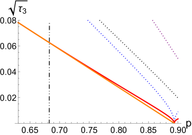
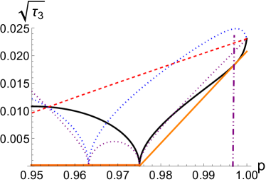
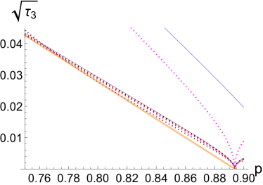
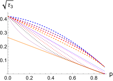
Figure 6: Convexification procedure where four different real solutions, both negative and positive, are present in the model. Here is shown a particular case for $\gamma=1$, $h=0.9$ and $\alpha=0.1\pi$, but this case is generic for this particular case of $\gamma=1$. The solutions $Z_{i}$ of the zero polytope (zero-states) are located at values $p_{i}=0.999142$, $0.998093$ (both solutions have positive sign), $0.567217$ , and $0.119002$ (both with negative sign); the respective tangle vanishes in between $0.893712$ and $0.975046$ Osterloh (2016a). The particular convexification points are indicated by dash-dot-dotted vertical lines at $p_{-}=0.656507$ and $p_{+}=0.997357$ in the first line of figures. Shown are the 1-1-decompositions with the first (black) to fourth (red) zero-state $|Z_{i}\rangle$ and their convexifications in orange. In the second row of figures (2,1)-decompositions are shown (dotted lines) where convex combinations of $|Z_{2}\rangle$ and $|Z_{4}\rangle$ are the disentangled part of the decomposition; they are all above the convexification.

In the cases we have inspected, the weight of the corresponding eigenstate was located within the strictly convex zones. We have therefore not implemented the convexification procedure into the algorithm.

Appendix D Case studies for the $3^{+}N$ an $3^{-}N$ scenario

Here we analyze exemplarily the state emerging as ground state for the values $h=0.5$, $\gamma=0.1$ and $\alpha=0.15708$ with a four tangle vector of $\vec{\tau}_{4}\approx(0.0802,0.0648,0.0934)$ with length $\tau_{4}\approx 0.1391$ in case of the $3^{+}N$ class and $\vec{\tau}_{4}\approx(0.0273,0.0393,0.0484)$ with length $\tau_{4}=0.0680$ in case of the $3^{-}N$ class. The corresponding $(2,1)$ and $(1,1)$ decompositions can be seen in Fig. 7. There, $\sqrt{\tau_{3}}$ is shown for the $(2,1)$ (red) and $(1,1)$ (blue and purple) decompositions for this specific case. The minimum is given by the black curve underneath. It is clearly seen that a convexification is needed.

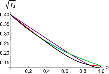
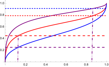
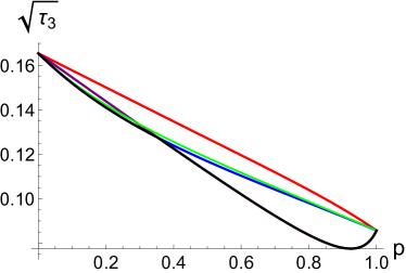
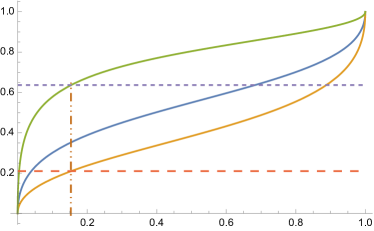
Figure 7: $\sqrt{\tau_{3}}$ is shown in the left panel for the $(2,1)$ (red) and $(1,1)$ (blue and purple) decompositions for a zero-polytope of classes $3^{+}N$ (upper row) and $3^{-}N$ (lower row). The minimum is given by the black curve underneath. It is clearly seen that a convexification is needed. This convexification leads for the $3^{+}N$ class to a single 3D simplex on top of each visible sides of the zero-polytope as a basis. This can be seen in the right panel of the plot where the piercing point of the central axis is plotted as a function of the $p$-value of the corresponding pure state as tip of that tetrahedron. For the class $3+N$, single pure states at $p$-values of $p_{N^{+}}\approx 0.8692$ and $p_{N^{-}}\approx 0.1296$ can be singled out. In the $3^{-}N$ class a single triangular tip at $p_{\Delta}\approx 0.1539$. Also here multiple states in the optimal decomposition would be indicated by multiple $p$-values for them in the right corresponding figure.

We have analysed whether deviations in $\phi$ direction are possible to lower the overall value for $\sqrt{\tau_{3}}$ with respect to $(1,1)$ decompositions. It is shown a light green curve which corresponds to $(1,2)$ decompositions with a yet considerable value of $\phi=0.5$. The growing of the weight function slightly overcompensates the gain one would have in the threetangle of the corresponding pure states. As argued earlier, a splitting in $p$ direction would immediately lead to linearization in a 3D simplex; this would lead to a linearization in an already stricly convex background and hence to a bigger value for $\sqrt{\tau_{3}}$.

In the first case, this convexification leads to a single 3D simplex on top of each visible sides of the zero-polytope as a basis which cut the central $z$-axis from $p_{\rm low}^{-}\approx 0.2487$ to $p_{\rm high}^{-}\approx 0.4476$ and from $p_{\rm low}^{+}\approx 0.7913$ to $p_{\rm high}^{+}\approx 0.9141$. This can be seen in the corresponding right panel of the plot where the piercing point of the central axis is plotted as a function of the $p$-value of the corresponding pure state as tip of that simplex. Indeed, single pure states at $p$-values of $p_{N^{+}}\approx 0.8692$ and $p_{N^{-}}\approx 0.1296$ can be singled out. Multiple pure states would be indicated by different corresponding values of $p$ for them.

The same procedure for a zero polytope of the $3^{-}N$ type leads to the curves plotted in the lower two plots in Fig. 7. Again, the left figure shows the curves for $(2,1)$ (red) and $(1,1)$ (blue and purple) decompositions, whereas on the right the convexification points are shown with $p^{-}\approx 0.2098$ and $p^{+}\approx 0.6368$. Both points coincide in a single pure state at $p_{\Delta}\approx 0.1539$.

References

- Ladd et al. (2010) T. D. Ladd, F. Jelezko, R. Laflamme, Y. Nakamura, C. Monroe, and J. L. O’Brien, Nature 464, 45 (2010).
- Gill et al. (2022) S. S. Gill, A. Kumar, H. Singh, M. Singh, K. Kaur, M. Usman, and R. Buyya, Software: Practice and Experience 52, 66 (2022).
- Orús et al. (2019) R. Orús, S. Mugel, and E. Lizaso, Reviews in Physics 4, 100028 (2019).
- Ringbauer et al. (2022) M. Ringbauer, M. Meth, L. Postler, R. Stricker, R. Blatt, P. Schindler, and T. Monz, Nature Physics 18, 1053 (2022).
- Narducci et al. (2022) F. A. Narducci, A. T. Black, and J. H. Burke, Advances in Physics: X 7, 1946426 (2022).
- Degen et al. (2017) C. L. Degen, F. Reinhard, and P. Cappellaro, Reviews of modern physics 89, 035002 (2017).
- Crawford et al. (2021) S. E. Crawford, R. A. Shugayev, H. P. Paudel, P. Lu, M. Syamlal, P. R. Ohodnicki, B. Chorpening, R. Gentry, and Y. Duan, Advanced Quantum Technologies 4, 2100049 (2021).
- Wang et al. (2023) Y. Wang, Z. Hu, and S. Kais, Photonic Quantum Technologies: Science and Applications 2, 651 (2023).
- Aslam et al. (2023) N. Aslam, H. Zhou, E. K. Urbach, M. J. Turner, R. L. Walsworth, M. D. Lukin, and H. Park, Nature Reviews Physics 5, 157 (2023).
- Schnabel et al. (2010) R. Schnabel, N. Mavalvala, D. E. McClelland, and P. K. Lam, Nature communications 1, 121 (2010).
- Pezze et al. (2018) L. Pezze, A. Smerzi, M. K. Oberthaler, R. Schmied, and P. Treutlein, Reviews of Modern Physics 90, 035005 (2018).
- Polino et al. (2020) E. Polino, M. Valeri, N. Spagnolo, and F. Sciarrino, AVS Quantum Science 2 (2020).
- Gisin and Thew (2007) N. Gisin and R. Thew, Nature photonics 1, 165 (2007).
- Luo et al. (2023a) W. Luo, L. Cao, Y. Shi, L. Wan, H. Zhang, S. Li, G. Chen, Y. Li, S. Li, Y. Wang, et al., Light: Science & Applications 12, 175 (2023a).
- Cozzolino et al. (2019) D. Cozzolino, B. Da Lio, D. Bacco, and L. K. Oxenløwe, Advanced Quantum Technologies 2, 1900038 (2019).
- De Santis et al. (2024) G. De Santis, K. Kravtsov, S. Amairi-Pyka, and J. A. Grieve, arXiv preprint arXiv:2406.08562 (2024).
- Horodecki et al. (2009) R. Horodecki, P. Horodecki, M. Horodecki, and K. Horodecki, Reviews of modern physics 81, 865 (2009).
- Gühne and Tóth (2009) O. Gühne and G. Tóth, Physics Reports 474, 1 (2009).
- Eltschka and Siewert (2014a) C. Eltschka and J. Siewert, Journal of Physics A: Mathematical and Theoretical 47, 424005 (2014a).
- Hein et al. (2004) M. Hein, J. Eisert, and H. J. Briegel, Physical Review A 69, 062311 (2004).
- Tóth and Gühne (2005) G. Tóth and O. Gühne, Physical review letters 94, 060501 (2005).
- Huber et al. (2010) M. Huber, F. Mintert, A. Gabriel, and B. C. Hiesmayr, Physical review letters 104, 210501 (2010).
- Huber and Sengupta (2014) M. Huber and R. Sengupta, Physical review letters 113, 100501 (2014).
- Milz et al. (2021) S. Milz, C. Spee, Z.-P. Xu, F. Pollock, K. Modi, and O. Gühne, SciPost Physics 10, 141 (2021).
- Vidal and Werner (2002) G. Vidal and R. F. Werner, Physical Review A 65, 032314 (2002).
- Jungnitsch et al. (2011) B. Jungnitsch, T. Moroder, and O. Gühne, Physical review letters 106, 190502 (2011).
- Wei and Goldbart (2003) T.-C. Wei and P. M. Goldbart, Physical Review A 68, 042307 (2003).
- Sen et al. (2010) A. Sen, U. Sen, et al., Physical Review A 81, 012308 (2010).
- Das et al. (2016) T. Das, S. S. Roy, S. Bagchi, A. Misra, A. Sen, U. Sen, et al., Physical Review A 94, 022336 (2016).
- Kondra et al. (2021) T. V. Kondra, C. Datta, and A. Streltsov, arXiv preprint arXiv:2111.12646 (2021).
- Blasone et al. (2008) M. Blasone, F. Dell’Anno, S. De Siena, and F. Illuminati, Physical Review A 77, 062304 (2008).
- Verstraete et al. (2003) F. Verstraete, J. Dehaene, and B. D. Moor, Phys. Rev. A 68, 012103 (2003).
- Osterloh and Siewert (2005) A. Osterloh and J. Siewert, Phys. Rev. A 72, 012337 (2005).
- Osterloh (2016a) A. Osterloh, Physical Review A 94, 062333 (2016a).
- D–oković and Osterloh (2009) D. Ž. D–oković and A. Osterloh, J. Math. Phys. 50, 033509 (2009).
- Osterloh and Siewert (2010) A. Osterloh and J. Siewert, New Journal of Physics 12, 075025 (2010).
- Gurvits (2003) L. Gurvits, in Proceedings of the thirty-fifth annual ACM symposium on Theory of computing (2003) pp. 10–19.
- Osterloh and Schützhold (2017) A. Osterloh and R. Schützhold, Physical Review A 96, 012331 (2017).
- Osterloh (2016b) A. Osterloh, Physical Review A 93, 052322 (2016b).
- Eltschka and Siewert (2014b) C. Eltschka and J. Siewert, Physical Review A 89, 022312 (2014b).
- Coffman et al. (2000) V. Coffman, J. Kundu, and W. K. Wootters, Phys. Rev. A 61, 052306 (2000).
- McCoy et al. (1971) B. M. McCoy, E. Barouch, and D. B. Abraham, Physical Review A 4, 2331 (1971).
- Wootters (1998) W. K. Wootters, Phys. Rev. Lett. 80, 2245 (1998).
- Viehmann et al. (2012) O. Viehmann, C. Eltschka, and J. Siewert, Applied Physics B 106, 533 (2012).
- Osterloh et al. (2008) A. Osterloh, J. Siewert, and A. Uhlmann, Phys. Rev. A 77, 032310 (2008).
- Neveling (2019) J. Neveling, 3-TANGLE VON RANG-2-ZUSTANDSGEMISCHEN IM LINEAREN XY-MODELL, Master’s thesis, University of Duisburg-Essen, Germany (2019).
- Eltschka et al. (2008) C. Eltschka, A. Osterloh, J. Siewert, and A. Uhlmann, New J. Phys. 10, 043014 (2008).
- Regula and Adesso (2016a) B. Regula and G. Adesso, Physical Review A 94, 022324 (2016a).
- Regula and Adesso (2016b) B. Regula and G. Adesso, Physical Review Letters 116, 070504 (2016b).
- Lohmayer et al. (2006) R. Lohmayer, A. Osterloh, J. Siewert, and A. Uhlmann, Phys. Rev. Lett. 97, 260502 (2006).
- (51) A. Osterloh, “More details on the threetangle in the xy-model class with a non-integrable field background,” To be published soon.
- Eltschka and Siewert (2012a) C. Eltschka and J. Siewert, Physical review letters 108, 020502 (2012a).
- Siewert and Eltschka (2012) J. Siewert and C. Eltschka, Physical review letters 108, 230502 (2012).
- Zhang and Nori (2023) Y.-R. Zhang and F. Nori, arXiv preprint arXiv:2304.00564 (2023).
- Cao et al. (2024) H. Cao, S. Morelli, L. A. Rozema, C. Zhang, A. Tavakoli, and P. Walther, Physical Review Letters 133, 150201 (2024).
- Malla et al. (2023) R. K. Malla, A. Weichselbaum, T.-C. Wei, and R. M. Konik, arXiv preprint arXiv:2310.05870 (2023).
- Wu et al. (2024) K. Wu, Z. Chen, Z.-P. Xu, Z. Ma, and S.-M. Fei, arXiv preprint arXiv:2406.07274 (2024).
- Li et al. (2024) R. Li, S. Zhang, Z. Qin, C. Du, Y. Zhou, and Z. Xiao, arXiv preprint arXiv:2408.13015 (2024).
- Iglói and Tóth (2023) F. Iglói and G. Tóth, Physical Review Research 5, 013158 (2023).
- Luo et al. (2023b) Y.-J. Luo, J.-M. Liu, and C. Zhang, Physical Review A 108, 052424 (2023b).
- Gulati et al. (2024) V. Gulati, S. Siyanwal, K. Dorai, et al., arXiv preprint arXiv:2409.19739 (2024).
- Eltschka and Siewert (2012b) C. Eltschka and J. Siewert, Scientific Reports 2, 942 (2012b).
- Carathéodory (1911) C. Carathéodory, Rendiconti Del Circolo Matematico di Palermo (1884-1940) 32, 193 (1911).
- Uhlmann (1998) A. Uhlmann, Open Syst. Inf. Dyn. 5, 209 (1998).
- Wong and Christensen (2001) A. Wong and N. Christensen, Phys. Rev. A 63, 044301 (2001).
- Cayley (1846) A. Cayley, Journal für reine und angewandte Mathematik 30, 1 (1846).
- Miyake and Wadati (2002) A. Miyake and M. Wadati, Quant. Info. Comp. 2, 540 (2002).