Gravitational Dark Matter Production in Supergravity $\alpha$-Attractor Inflation

Abstract

We consider gravitational particle production (GPP) of dark matter (DM) under supergravity framework, where $\alpha$-attractor inflation model is used. The particle spectrum is computed numerically and the dark matter number density is obtained. We show how the dark matter mass, gravitino mass and inflation model parameters modify the results, and find the corresponding reheating temperature which leads to sufficient DM production. In our setup, supergravity corrections suppress the efficiency of GPP, and make the isocurvature constraint much weaker compared with the normal case. With tensor to scalar ratio ranges from $10^{-3}-10^{-4}$, and dark matter mass from $10^{-2}m_{\phi}-m_{\phi}$, the required reheating temperature should be around $10^{3}\textrm{GeV}-10^{7}\textrm{GeV}$.

1 Introduction

Based on current observations, our Universe is almost isotropic and presumably also homogeneous. It contains dark matter (DM) that interacts weakly with ordinary matter Planck:2018vyg . Inflation, where the Universe experiences a period of accelerated expansion, provides an excellent explanation to this isotropy and homogeneity Linde:1981mu ; Albrecht:1982wi . The quantum fluctuations of inflaton field also seed the initial conditions for structure formation. In addition, inflation can source particle production; one example is the so-called gravitational particle production (GPP), where time evolution of the background spacetime leads to the production Lyth:1996yj ; Chung:1998zb .

GPP is inevitable for any degree of freedom as long as it couples to gravity. This production channel can contribute significantly to dark matter abundance, and generate isocurvature perturbation. For a comprehensive review, we refer the review Kolb:2023ydq . If gravity is the only interaction between DM and Standard Model (SM) particles, DM from GPP will never be in thermal equilibrium with the rest of particles, unlike canonical thermal freeze-in or freeze-out mechanism. GPP has been extensively studied in the past two decades, leading to a rich phenomenology in scalar and higher spin fields Lyth:1996yj ; Chung:1998ua ; Kolb:1998ki ; Mukhanov:2005sc ; Ling:2021zlj ; Garcia:2023qab ; Kuzmin:1998kk ; Chung:2011ck ; Graham:2015rva ; Ahmed:2020fhc ; Kolb:2020fwh ; Gorghetto:2022sue ; Cembranos:2023qph ; Ozsoy:2023gnl ; Hasegawa:2017hgd ; Kallosh:1999jj ; Antoniadis:2021jtg ; Kaneta:2023uwi ; Casagrande:2023fjk ; Kolb:2023dzp ; Nilles:2001ry ; Nilles:2001fg . Meanwhile, analytic treatments to track particle productions have been developed in certain cases Chung:1998bt ; Ema:2018ucl ; Cembranos:2019qlm ; Enomoto:2020xlf ; Basso:2021whd ; Hashiba:2021npn ; Basso:2022tpd ; Kaneta:2022gug ; Racco:2024aac ; Verner:2024agh ; Jenks:2024fiu .

Even though the precise results of GPP depend on the inflation model, some general statements can be made without specifying inflation dynamics. For a scalar field $\chi$ lighter than the inflation scale $H_{I}$, its number density spectrum will feature an infra-red (IR) divergence, which has to be regulated through a cut-off in momentum space. Its isocurvature spectrum will be almost scale invariant, which might go conflicts with CMB observations. On the contrast, if the field is heavier than $H_{I}$, its number density will be convergent without cut-off and the isocurvature signal can be negligible.

Due to the weak nature of gravity, the above conclusion can be easily modified. Corrections may appear from various sources. Introducing non-minimal coupling between DM and gravity can greatly change the efficiency of GPP. A conformal coupled scalar experiences less GPP, has no IR divergence and leaves negligible isocurvature at CMB scale, larger interaction will enhance the GPP production Markkanen:2015xuw ; Fairbairn:2018bsw ; Cembranos:2019qlm ; Clery:2022wib ; Garcia:2023qab ; Yu:2023ity . Introducing direct coupling between inflaton field and DM leads to a similar effects Garcia:2022vwm ; Garcia:2023awt . In this paper we would like to focus on another possibility, where such correction comes from supergravity (SUGRA) effects.

SUGRA is the local gauge theory of supersymmetry (SUSY), which generally predicts non-renormalizable interactions between inflaton field and DM field. These interactions can play a significant role in cosmology Endo:2006qk ; Endo:2006nj ; Endo:2007sz ; Enomoto:2013mla ; Ema:2024sit . Previous study in SUGRA GPP focused on the case where $m_{\chi}>H_{I}$ Nakayama:2019yjv , and we would like to have a comprehensive understanding over different parameter spaces. Even for light DMs, SUGRA correction makes their effective mass naturally larger than Hubble scale. This correction has the same origin as the $\eta$ problem in SUGRA inflation research Copeland:1994vg .

In this paper, we focus on $\alpha$-attractor model, which is realized in SUGRA using a stabilizer field DallAgata:2014qsj ; Kallosh:2014hxa . This framework also allows us to introduce arbitrary SUSY breaking scale $m_{3/2}$. Even though for canonical choice of $m_{3/2}\sim\textrm{TeV}$, its impact on GPP can be safely neglect. It is still interesting to investigate how a larger $m_{3/2}$ could alert GPP. We numerically calculate the number density of a scalar DM, as well as its isocurvature contribution. Compared with non-SUSY GPP, SUGRA models need a higher reheating temperature to produce the same amount of DM.

This paper is organized as follows. In section 2, we introduce the inflation model, basics of GPP, and eventually how to embed our model in SUGRA framework. The numerical results of GPP are presented in section 3 and possibly observational consequences are discussed. Section 4 contains conclusion and outlook of this work.

2 Theoretical framework of GPP and SUGRA GPP

2.1 Inflation model

Inflation is assumed to be a period of quasi-de Sitter spacetime. The simplest realization is single-field slow-roll inflation, where the assumed (scalar) field slows down dramatically. The kinetic energy is negligible compared to the potential energy and therefore the equation of state becomes $\omega\approx-1$. This leads the Universe to expand exponentially. The equation of motion of the inflaton field and Friedmann equations of first and second kind expressed in conformal time $\tau$ are

$$\phi^{\prime\prime} +2\mathcal{H}\phi^{\prime}+a^{2}\partialderivative{V}{\phi}=0,$$ (1a)

$$\mathcal{H}^{2} =\left(\frac{a^{\prime}}{a}\right)^{2}=\frac{1}{3}\left(\frac{1}{2}\phi^{\prime 2}+a^{2}V\right),$$ (1b)

$$\frac{a^{\prime\prime}}{a} =\frac{1}{6m_{\text{pl}}^{2}}\left(4a^{2}V-\phi^{\prime 2}\right),$$ (1c)

where prime denotes derivative with respect to the conformal time.

The (potential) slow-roll parameters are given by the first and second derivative of the inflaton potential

$$\epsilon_{V}=\frac{1}{2m_{\text{pl}}^{2}}\left(\frac{V^{\prime}}{V}\right)^{2},\quad\eta_{V}=\frac{1}{m_{\text{pl}}^{2}}\frac{V^{\prime\prime}}{V}.$$ (2)

Here we denote $V^{\prime}=\differential{V}/\differential{\phi}$. It can be shown slow-roll inflation happens when $\epsilon,|\eta_{V}|\ll 1$.

In this work, we choose to work with T model $\alpha$-attractor as our inflation model, which can be easily realized in the SUGRA context, see section 2.3. It has the following potential Kallosh:2013yoa

$$V_{I}(\phi)=V_{0}\tanh^{2n}{\left(\frac{\phi}{\sqrt{6\alpha}}\right)}.$$ (3)

In this work, $n=1$ is used throughout. The slow roll parameters for this model are

$$\epsilon_{V} =\frac{2n^{2}}{\sinh(\phi/\sqrt{6\alpha})\cosh(\phi/\sqrt{6\alpha})}$$ (4)

$$\eta_{V} =\frac{1}{6\alpha}\frac{2(1-\tanh^{2}(\phi/\sqrt{6\alpha}))-6\tanh^{2}(\phi/\sqrt{6\alpha})(1-\tanh^{2}(\phi/\sqrt{6\alpha}))}{\tanh^{2}(\phi/\sqrt{6\alpha})}$$ (5)

The spectral index of the scalar perturbation $n_{s}$ can be given by the two potential slow-roll parameters at the CMB scale

$$n_{s}-1=2\eta_{*}-4\epsilon_{*}.$$ (6)

It has to be consistent with the observed value of $n_{s}=0.965\pm 0.004$ Planck:2018vyg . One can use this to compute the field value $\phi_{*}$ at the CMB scale Germ_n_2021

$$\cosh^{2}\left(\frac{\phi_{*}}{\sqrt{6\alpha}}\right)=\frac{1}{2(1-n_{s})}\left(1-n_{s}+\frac{4}{3\alpha}+\sqrt{(1-n_{s})^{2}+\frac{8}{3\alpha}(1-n_{s})+\frac{16}{9\alpha^{2}}}\right).$$ (7)

We can rewrite the potential parameter $\alpha$ in terms of observables. When fixing the tensor-to-scalar ratio and spectral index, we have

$$\alpha=\frac{64}{3}\frac{r}{(8(1-n_{s})-r)^{2}-r^{2}}.$$ (8)

As we only have a upper bound on $r$, $\alpha$ also only has a upper bound. At last, the “scale” of the potential $V_{0}$ can be determined by the normalization of the power spectrum Planck:2018jri

$$\mathcal{A}=\frac{1}{24\pi^{2}}\left.\frac{V}{\epsilon}\right|_{\phi=\phi_{*}}\stackrel{{\scriptstyle!}}{{=}}2.1\cdot 10^{-9}.$$ (9)

Another important scale is the infalton mass, which reads

$$m_{\phi}^{2}=\left.\partialderivative[2]{V}{\phi}\right|_{\phi=0}=\frac{V_{0}}{3\alpha}.$$ (10)

As a result, we have in this model $m_{\phi}^{2}/H_{\text{inf}}^{2}=1/\alpha$ which can be much smaller than unity, especially if the bound for tensor-to-scalar ratio is lowered in the future.

The end of slow-roll inflation is marked by either one of the magnitude of slow roll parameters being unity

$$2\cosh^{2}\left(\frac{\phi_{e}}{\sqrt{6\alpha}}\right)=\begin{cases}1+\frac{2}{3\alpha}+\sqrt{1+\frac{8}{3\alpha}\left(\frac{1}{6\alpha}-1\right)},&\alpha\leq\alpha_{l}\\ 1+\sqrt{1+\frac{4}{3\alpha}},&\alpha>\alpha_{l}\end{cases},$$ (11)

with $\alpha_{l}\approx 0.17$ for $n=1$.

2.2 Gravitational Particle Production

In addition to the inflaton field, we also assume there exists a spectator scalar field $\chi$ with the following action

$$S_{\chi}=-\frac{1}{2}\int\differential[4]{x}\sqrt{-g}\left(2\xi\chi^{2}R+g^{\mu\nu}\partial_{\mu}\chi\partial_{\nu}\chi+m_{\chi}^{2}\chi^{2}\right),$$ (12)

where $g$ is the determinant of $g^{\mu\nu}$ and $R$ is the Ricci scalar. Higher order self-interactions of $\chi$ have been neglected and $m_{\chi}^{2}$ could be a function of other fields. Here, we use the FLRW metric with conformal time

$$g_{\mu\nu}\differential{x^{\mu}}\differential{x^{\nu}}=a^{2}(\tau)\left(\differential{\tau}^{2}-\differential{\vec{x}^{2}}\right).$$ (13)

The field is rescaled $\tilde{\chi}=a\chi$. Then, after Fourier decomposing the field $\tilde{\chi}$, the equation of motion for $\tilde{\chi}$ field turns into the equation for the mode function

$$\tilde{\chi}_{k}^{\prime\prime}+\omega^{2}_{k}\tilde{\chi}_{k}=0,\quad\omega_{k}^{2}=k^{2}+a^{2}m_{\chi,\text{eff}}^{2}=k^{2}+a^{2}m_{\chi}^{2}-(1-6\xi)\frac{a^{\prime\prime}}{a}.$$ (14)

In this work, we only consider vanishing conformal coupling $\xi=0$. In the case where $\omega^{2}_{k}$ varies rapidly, the field $\chi$ can get excited and particles are produced.

The same phenomenon can also be understood in terms of the Bogoliubov coefficients. Assume that the spacetime are asymptotically flat at early and late times. The Bogoliubov coefficients describes how the orthonormal basis functions at these times relate to each other. The equation (14) can be formulated in terms of the Bogoliubov coefficients

$$\alpha^{\prime}_{k}v_{k}=\frac{\omega^{\prime}_{k}}{2\omega_{k}}v_{k}^{*}\beta_{k},\quad\beta^{\prime}_{k}v_{k}^{*}=\frac{\omega^{\prime}_{k}}{2\omega_{k}}v_{k}\alpha_{k},$$ (15)

with

$$v_{k}(\tau)=\frac{1}{\sqrt{2\omega_{k}}}\exp(-i\int\omega_{k}\differential{\tau}).$$ (16)

It proves to be more efficient numerically to solve for these instead of the mode functions.

The number density spectrum is given by

$$f_{\chi}(k,\tau)=|\beta(k,\tau)|^{2},$$ (17)

and the comoving number density can be obtained from it

$${a}^{3}n_{\chi}=\frac{1}{2\pi^{2}}\int\differential{k}k^{2}|\beta_{k}|^{2}.$$ (18)

We assume that the comoving number density doesn’t change after production and they are always the cold dark matter .

Using normal ordering to cure the UV divergence, the final energy density can be approximated as

$$a^{3}\rho_{\chi}\approx\frac{1}{2\pi^{2}a^{4}}\int\differential kk^{2}|\beta_{k}|^{2}\omega_{k},$$ (19)

where we only include terms up to second order in $|\beta_{k}|$ and ignore the terms suppressed by Hubble parameter and Ricci scalar (decays away quickly).

The isocurvature power spectrum is defined as

$$\Delta_{\delta}^{2}(k)=\frac{1}{\rho^{2}}\frac{k^{3}}{2\pi^{2}}\int\differential[3]{r}e^{-i\vec{k}\cdot\vec{r}}\expectationvalue{\delta\hat{\rho}(0)\delta\hat{\rho}(\vec{r})},$$ (20)

where time-dependence has been ignored. It can be written in terms of the mode functions Chung_2005 ; Ling:2021zlj ; Kolb:2023ydq

$$\begin{split}\Delta_{\delta}^{2}(\eta,k)&=\frac{1}{a^{8}\bar{\rho}^{2}}\frac{k^{3}}{(2\pi)^{5}}\int\differential[3]{k^{\prime}}\Big{[}|\partial\chi_{k^{\prime}}|^{2}|\partial\chi_{|\boldsymbol{k}^{\prime}-\boldsymbol{k}|}|^{2}+a^{4}m^{4}|\chi_{k^{\prime}}|^{2}|\chi_{|\boldsymbol{k}^{\prime}-\boldsymbol{k}|}|^{2}\\ &\quad+a^{2}m^{2}\left(\chi_{k^{\prime}}\partial\chi_{k^{\prime}}^{*}\chi_{|\boldsymbol{k}^{\prime}-\boldsymbol{k}|}\partial\chi_{|\boldsymbol{k}^{\prime}-\boldsymbol{k}|}^{*}+\chi_{k^{\prime}}^{*}\partial\chi_{k^{\prime}}\chi_{|\boldsymbol{k}^{\prime}-\boldsymbol{k}|}^{*}\partial\chi_{|\boldsymbol{k}^{\prime}-\boldsymbol{k}|}\right)\Big{]}\end{split}$$ (21)

Instead, it can be reformulated using the Bogoliubov coefficients and momenta can be relabeled at $(k,k^{\prime},|\boldsymbol{k}^{\prime}-\boldsymbol{k}|)\rightarrow(k,p,q)$ Garcia:2023awt

$$\Delta_{\delta}^{2}(k)=\frac{a_{e}^{2}m_{\chi}^{2}}{(a_{e}^{4}\rho)^{2}}\frac{2k^{2}}{(2\pi)^{4}}\int_{0}^{\infty}\differential{p}p\int_{|k-p|}^{k+p}\differential{q}q\left[|\beta_{p}|^{2}|\alpha_{q}|^{2}+\Re{\alpha_{p}^{*}\beta_{p}\alpha_{q}\beta_{q}^{*}e^{2i\Phi_{p}-2i\Phi_{q}}}\right]$$ (22)

where the time-dependence has been omitted as we are only interested in the final spectrum.

2.3 SUGRA Embedment

In this section we will discuss how to realize inflation in supergravity framework. In supergravity, scalar potential is generated by a Kähler potential $\mathcal{K}$ and Superpotential $\mathcal{W}$, both of them are functions of superfields $\Phi^{\alpha}$, where $\alpha$ refers to different superfields in the theory. Note Kähler potential $\mathcal{K}$ is a hermitian function while superpotential $\mathcal{W}$ is a holomorphic function. In the scalar part, Kähler potential determines the kinetic function of scalar fields and controls the scalar potential together with superpotential (We use Planck units in this section $m_{\text{pl}}=1$).

$$\begin{split}\sqrt{-g}\mathcal{L}&=-\mathcal{K}_{\alpha\overline{\beta}}\partial_{\mu}\phi^{\alpha}\partial^{\mu}\bar{\phi}^{\overline{\beta}}-V\\ V&=e^{{\cal K}}({\cal K}^{\alpha\overline{\beta}}D_{\alpha}{\cal W}\overline{D_{\beta}{\cal W}}-3|{\cal W}|^{2})\,,\end{split}$$ (23)

where $\phi^{\alpha}$ is the spin-0 component of superfield $\Phi^{\alpha}$. $\mathcal{K}_{\alpha\overline{\beta}}=\frac{\partial^{2}\mathcal{K}}{\partial\phi^{\alpha}\partial\bar{\phi}^{\bar{\beta}}}$ is the Kähler metric, and $\mathcal{K}^{\alpha\overline{\beta}}$ is the inverse of it. $D_{\alpha}\mathcal{W}=\frac{\partial\mathcal{W}}{\partial\phi^{\alpha}}+\frac{\partial\mathcal{K}}{\partial\phi^{\alpha}}\mathcal{W}$ is the Kähler covariant derivative. Existence of $e^{\mathcal{K}}$ in the scalar potential leads to the so called $\eta$ problem in the early study of supergravity inflation Copeland:1994vg . For any field with canonical Kähler potential $\mathcal{K}=\bar{\Phi}\Phi$, the second order derivative of the potential:

$$\frac{\partial^{2}V}{\partial\phi\partial\phi}\sim V+\textrm{others}...$$ (24)

leads to a $\mathcal{O}(1)$ slow roll parameter $\eta=V^{\prime\prime}/V\sim 1$. This holds true for both possible inflaton field and any other fields present in the Kähler potential. In this paper, we will assume this correction indeed exist for dark matter field, which means DM get a effective mass in order of Hubble scale. As we will show in this paper, this significantly alter the results for GPP production of DM fields.

One elegant solution of $\eta$ problem is shift symmetry, by which the inflaton field doesn’t appear in the Kähler potential. In this way, one can realize most of the inflation models Kallosh:2010xz . To embed the aforementioned inflation model in supergravity, we use the formalism proposed in DallAgata:2014qsj ; Kallosh:2014hxa , which can accommodate arbitrary inflationary model with arbitrary supersymmetry (SUSY) breaking scale. It essentially has three superfields: the inflaton field $\Phi$, the stabilizer field $S$ and the DM field $\chi$, with the following Kähler potential $\mathcal{K}$ and Superpotential $\mathcal{W}$

$$\begin{split}\mathcal{K}(\Phi,S,\chi)&=-\frac{1}{2}(\Phi-\bar{\Phi})^{2}+S\bar{S}+\chi\bar{\chi},\\ \mathcal{W}(\Phi,S,\chi)&=f(\Phi)+Sg(\Phi)+\frac{1}{2}m_{\chi}\chi^{2}.\end{split}$$ (25)

We also assume both $\textrm{Im}(\Phi),S,\chi=0$ during inflation as in Kallosh:2010xz . The Kähler covariant derivative of each field reads

$$\begin{split}D_{\Phi}W&=f^{\prime}(\Phi)+g^{\prime}(\Phi)S-(\Phi-\bar{\Phi})W,\\ D_{S}W&=g(\Phi)+\bar{S}W,\\ D_{\chi}W&=m_{\chi}\chi+\bar{\chi}W.\end{split}$$ (26)

We set $g(\Phi)=\sqrt{3}f(\Phi)$ and the scalar potential reads

$$V=e^{K}\left(K^{\alpha\bar{\beta}}{D_{\alpha}W}\overline{D_{\beta}W}-3\absolutevalue{W}^{2}\right).$$ (27)

Up to second order in $\chi$ and ignore the contribution form $\textrm{Im}(\Phi)$ and $S$, we have

$$\begin{split}V_{\chi}=e^{K}\Big{(}&m_{\chi}^{2}\chi\bar{\chi}+\frac{1}{4}m_{\chi}^{2}\chi^{2}\bar{\chi}^{2}+\frac{1}{4}m_{\chi}^{2}\chi^{3}\bar{\chi}^{3}\\ &-\frac{1}{2}m_{\chi}\bar{\chi}^{2}f+\frac{1}{2}m_{\chi}\chi\bar{\chi}^{3}f-\frac{1}{2}m_{\chi}\chi^{2}\bar{f}+\frac{1}{2}m_{\chi}\chi^{3}\bar{\chi}\bar{f}\\ &+\chi\bar{\chi}f\bar{f}+f^{\prime}\bar{f^{\prime}}\Big{)},\end{split}$$ (28)

where $V_{I}(\phi)=\absolutevalue{f^{\prime}(\Phi)}^{2}$ is the inflationary potential and $\phi=\sqrt{2}\textrm{Re}(\Phi)$ is the actual inflaton.

Accordingly, the inflationary potential (3) has the following $f$ function (with $n=1$)

$$f(\Phi)=\sqrt{3\alpha V_{0}}\log\left(\cosh(\frac{\Phi}{\sqrt{3\alpha}})\right)+\frac{m_{3/2}}{\sqrt{3}}.$$ (29)

In terms of DM field, We can split the complex field into two real fields $\chi=(\chi_{R}+i\chi_{I})/\sqrt{2}$ with the following mass term:

$$m_{\chi,R}^{2} =m_{\chi}^{2}+V_{I}+|f|^{2}-m_{\chi}f,$$ (30a)

$$m_{\chi,I}^{2} =m_{\chi}^{2}+V_{I}+|f|^{2}+m_{\chi}f,$$ (30b)

where we have used $f\in\mathbb{R}$ as only $\textrm{Re}(\Phi)$ is non-zero and there is no mixing between the real and imaginary parts. After the rescaling $\tilde{\chi}_{i}=a\chi_{i}$, their effective masses read

$$m_{\tilde{\chi},\text{eff}}^{2}=a^{2}\left(m_{\chi}^{2}+H^{2}+|f|^{2}\mp m_{\chi}f\right).$$ (31)

3 Numerical results

In this section we show the necessary numerical results for calculation of DM relic abundance in the current universe. The first step is to solve the background evolution of inflaton field through equations (1). In practice, we use the slow-roll solution as initial conditions for the inflaton field. As the inflation model is an attractor, the trajectory converges to the “true” one after sufficient time.

By choosing the above condition for the background, we also need to ensure that every mode is well inside the horizon upon simulation start and can be described by the Bunch-Davies vacuum

$$\chi_{k}=\frac{1}{\sqrt{2\omega_{k}}},\;\chi^{\prime}_{k}=\frac{-i\omega_{k}}{\sqrt{2\omega_{k}}},\quad\text{or equivalently,}\quad\alpha=1,\;\beta=0,$$ (32)

where $\omega_{k}$ is taken at the time of initialization and it approaches $k$ in the infinite past $\tau\rightarrow-\infty$. This means longer wavelength modes need to be initialized earlier. The smallest scale considered here is $k=10^{-2}\cdot a_{e}H_{e}$, and it requires initialization at $\sim 10$ e-folds before the end of inflation.

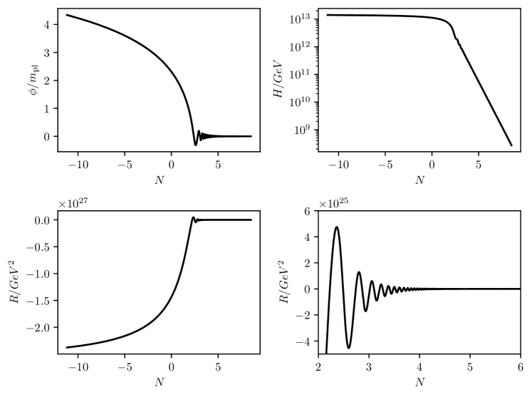
Figure 1: Background evolution: inflaton field value $\phi$, Hubble parameter $H$ and Ricci scalar $R$, with $\alpha\approx 1.0$ corresponding to would-be tensor to scalar ratio $r=0.0035$. The time variable has been transformed to number of $e$-folds $N(t)=\ln(a(t))$.

We show the relevant background quantities in figure 1. This is done using the inflation potential given in equation (3) with a fixed tensor to scalar ratio $r=0.0035$ ($\alpha\approx 1$). When plotting the variables, we use the number of $e$-folds $N=\ln a(t)$, instead of the cosmic time $t$, as the time variable. The scale factor has been rescaled so that the scale factor at end of inflation is unity $a(t_{e})\equiv 1$, which was chosen by the condition that the first Hubble slow-roll parameter equals $0.1$

$$\epsilon_{1}=-\frac{\dot{H}}{H^{2}}=\frac{1}{2m_{\text{pl}}^{2}}\left(\derivative{\phi}{N}\right)^{2}\stackrel{{\scriptstyle!}}{{=}}0.1.$$ (33)

Thus, the number of $e$-folds at the end of inflation is defined as zero. The first diagram shows the evolution of the field value $\phi(N)$. It smoothly rolls down to the minimum at $\phi=0$ and starts to oscillate around it. This oscillation process induces the decrease of Hubble scale $H$ as well as an oscillation of the Ricci scalar $R$. During slow roll inflation, both two quantities are more or less constants:

$$R=-6\frac{a^{\prime\prime}}{a^{3}}\approx-12H^{2}.$$ (34)

However, Ricci scalar oscillate around zero after inflation, and the Hubble $H$ oscillates much mildly than Ricci scalar due to the kinetic energy of inflaton field. Note that the Ricci scalar $R$ appears in the effective mass for non-SUGRA case in equation (14), and the Hubble parameter $H$ for the SUGRA case in equation (31).

Let us first consider effective frequency squared without SUGRA correction; it takes the following form

$$\omega_{k}^{2}=k^{2}+a^{2}m_{\chi}^{2}-\frac{a^{\prime\prime}}{a}=k^{2}+a^{2}\left(m_{\chi}^{2}+\frac{R}{6}\right)\stackrel{{\scriptstyle\text{SR}}}{{=}}k^{2}+a^{2}\left(m_{\chi}^{2}-\frac{2}{\alpha}m_{\phi}^{2}\right),$$ (35)

where the second Friedman equation in equations (34) have been used. The last equality only holds during slow roll inflation. For light DM field, the oscillation of $R$ leads the $\omega_{k}^{2}$ crosses zero and induce tachyonic instability, especially for low momentum modes.

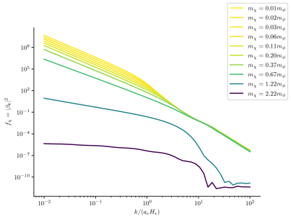
Figure 2: Phase space distribution of $\chi$ quanta without SUGRA correction. In the vanishing mass limit, the phase space distribution approaches $|\beta_{k}|^{2}\propto k^{-3}$.

One can then solve the differential equation associated with $\omega_{k}$ to get the phase space distribution of DM field. It proves to be more efficient to use equation (14) due to the tachyonic instability. We show some examples with different DM mass in figure 2. For light fields, the effects of tachyonic instability is significant, which leads to the typical scaling behavior in the low momentum region $f_{\chi}\propto k^{3}$. On the contrast, for heavier DM field, $f_{\chi}$ approaches a constant for similar momentum. The threshold DM mass is roughly the inflaton mass, as expected from equation (35). Heavier DM fields are generally harder to get excited. Their $f_{\chi}$ are much smaller than light fields.

Now let us consider the gravitational particle production of DM particles with SUGRA correction. The spectra with two distinct $m_{3/2}$’s are shown in figure 3. The most striking feature is that the spectrum has no infrared divergence. Due to the additional terms in effective mass in equation (31), the tachyonic instability doesn’t exist in SUGRA case. Again, higher $m_{\chi}$ gives less $\chi$ particles. When $m_{\chi}\ll m_{3/2}$, the spectra is controlled by the inflation potential and size of $m_{3/2}$. All light fields share basically indistinguishable spectra.

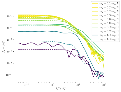
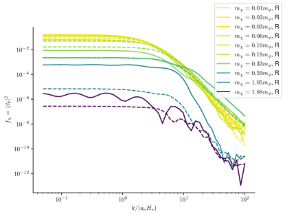
Figure 3: Phase space distribution of $\chi$ quanta with $m_{3/2}=0$ (left) and $m_{3/2}=0.1m_{\phi}$ (right). Dashed line represents the imaginary field and solid line the real field.

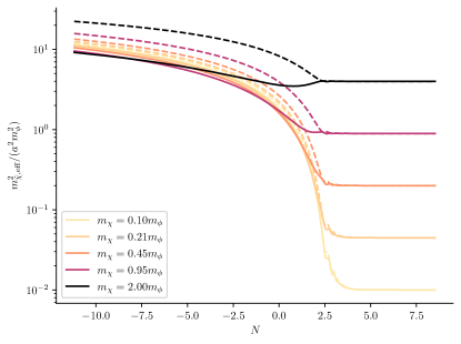
Figure 4: Effective mass squred in the appropriate units with $m_{3/2}=0.0$ (left) and $m_{3/2}=0.1\cdot m_{\phi}$ (right) respectively. Solid (dashed) line is for effective mass of real (imaginary) field.

We show the effective mass of DM fields during and after inflation in figure 4. The imaginary field has higher mass during inflation and the rate of change in effective frequency is higher for $m_{\chi}<m_{\phi}$. Thus, as one can see from the figure 3, in SUGRA the imaginary part has higher production in this region. On the contrary, for $m_{\chi}\gtrsim m_{\phi}$, the real part is produced in greater amount. When $m_{3/2}\ll\alpha m_{\phi}$, The mass splittings prior to reheating are similar among $m_{3/2}$’s, as the first term in the $f$-function dominates, see equation (29). Despite the splittings at the end of the particle production clearly depends on the gravitino mass

$$m_{\chi,R,I}^{2}=m_{\chi}^{2}+\frac{m_{3/2}^{2}}{3}\mp\frac{m_{3/2}m_{\chi}}{\sqrt{3}},$$ (36)

the ultimate rate of change for $m_{\chi,\text{eff}}^{2}$ and $\omega_{k}^{2}$ are largely unaffected by it. Thus, the phase space distributions are very similar with light gravitino masses.

From the phase space distribution, the isocurvature spectrum can be calculated via equation (5). The expectation is that $|\beta_{k}|^{2}\propto k^{-3}$ produces near scale-invariant isocurvature spectrum Kolb_2023 . In the vanishing mass limit $m_{\chi}\rightarrow 0$, the isocurvature spectrum indeed approaches scale invariance, see figure 5(a). This can be potentially dangerous when considering CMB isocurvature constraints Ling:2021zlj . In the SUGRA case, the isocurvature spectrum always holds a $k^{3}$ scaling in the low momentum limit. The spectra are shown in figure 5(b). Thus, the CMB isocurvature constraint poses no limitation on the model parameters.

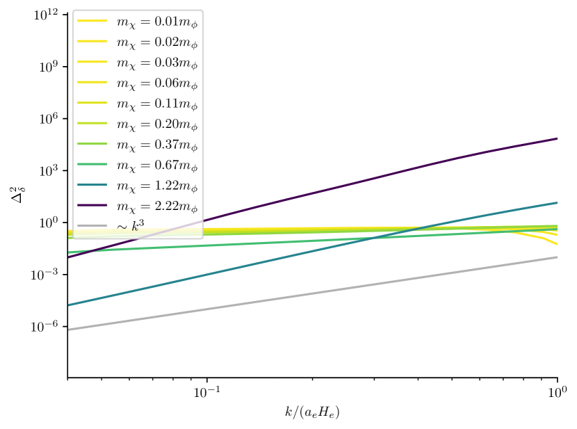
(a) Without SUGRA correction. Computed from the phase space distribution shown in figure 2.

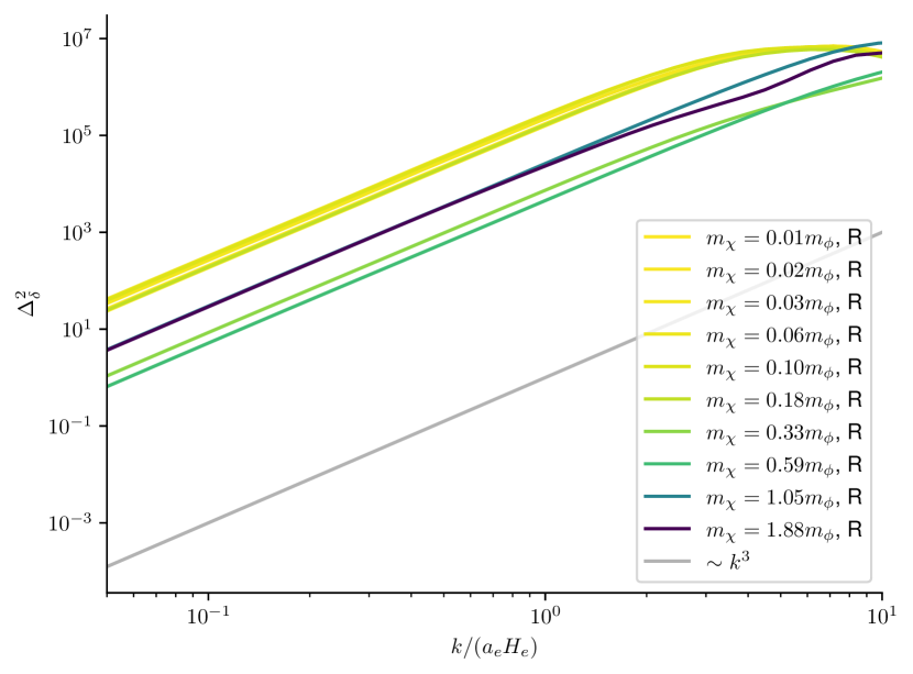
(b) With SUGRA correction and $m_{3/2}=0.0$. Computed from the phase space distribution shown in figure 3. Only the real field contributions are shown here.

Figure 5: Isocurvature power spectrum calculated using equation (22).

We show the energy densities of DM in the current universe in figure 6. We assume that the DM particle does not interact with other (standard model) particles and their comoving number density is conserved after production. Thus, its current energy density can be expressed as $\rho_{\chi,0}\approx m_{\chi}n_{\chi}$. On the vertical axis, we use the energy density of the DM particles divided by the entropy density and reheating temperature $\rho/(s_{0}T_{\text{rh}})$. This quantity is obtained from comoving number via the equation (43). To get the desired relic abundance $\Omega_{\textrm{DM}}h^{2}\approx 0.12$, we need

$$\frac{\rho_{\chi}(t_{0})}{s_{0}}\approx$4\text{\cdot}{10}^{-10}\text{\,}\mathrm{GeV}$.$$ (37)

This means different $m_{\chi}$’s will need different reheating temperature to satisfy this condition.

The phase space distribution of non-SUGRA case scales like $k^{-3}$ in the infra-red limit. This leads to an IR divergence in the total number density equation (18) with $n\sim\int_{0}^{\infty}\differential{k}k^{-1}$. To cure this divergence, one can set an IR cutoff at CMB scale, since (DM) perturbations larger than the horizon at recombination are just part of the background. As it is expensive to track modes across so many number of $e$-folds in our numerical computation, we choose to extrapolate the phase space distribution to the CMB scale. We take $60$ $e$-folds of inflation since CMB scale. It can be shown that the final abundance is proportional to the number of $e$-folds, if the number of $e$-folds is chosen differently. The abundance without SUGRA correction can be found in figure 6. As we see, the abundance saturates at the low mass limit, as expected from the phase space distribution in figures 2. The tachyonic instability goes away with increasing $m_{\chi}$, therefore, the abundance decreases rapidly.

The number density with SUGRA correction is more straightforward to compute and it is shown in figure 6 with $r=0.0035$. When $m_{\chi}<m_{\phi}$, the abundance from GPP increases with $m_{\chi}$ linearly, which comes from the linear mass dependency in energy density of non-relativistic particles. The abundance then decreases exponentially when $m_{\chi}>m_{\phi}$. There is an interesting bump for small $m_{3/2}$ around $m_{\chi}\sim m_{\phi}$. This primarily comes from the real field contribution, and one can see this for $k/(a_{e}m_{\phi})\gtrapprox 1$ also in figure 3.

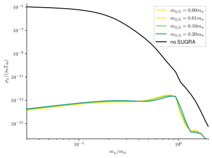
Figure 6: Comoving energy density of the DM field $\chi$ divided by the reheating temperature. Higher values require lower reheating temperatures. The tensor-to-scalar ratio is fixed to $r=0.0035$.

The abundances with various desired values of tensor-to-scalar ratio are plotted in figure 7. As we wish $\chi$ to be the only DM around, equation (43) leads to certain reheating temperature for a set of fixed model parameters ($m_{3/2}$, $m_{\chi}$ and $r$). As implied in figure 6, required reheating temperature $T_{\text{rh}}$ for all values of $r$ goes like $m_{\chi}^{-1}$ for small $m_{\chi}$ until $m_{\chi}\sim m_{\phi}$, where the produced comoving number density drops dramatically and high reheating temperature is necessary. Effects of $m_{3/2}$ is still very minimal. Lower desired tensor-to-scalar ratio demands higher reheating temperature, since the comoving number density drops with $r$ (however, $H_{e}^{2}$ gives additional parameter dependence).

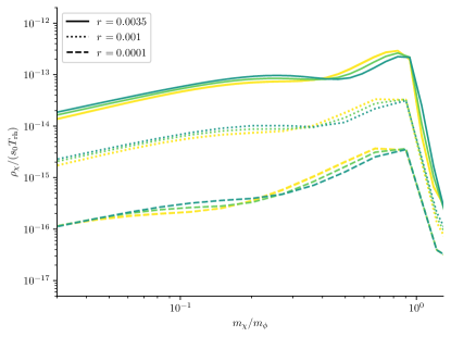
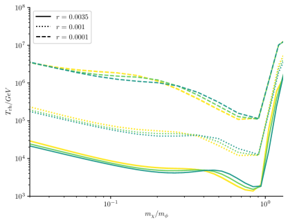
Figure 7: Dark matter abundance $\rho/(s_{0}T_{\text{rh}})$ and required reheating temperature for $\chi$ to be the only dark matter. Color corresponds to $m_{3/2}$, c.f. figure 6.

4 Conclusion and outlook

In this work, we looked at gravitationally produced dark matter particles with SUGRA correction. The $\alpha$-attractor inflation model was chosen for this investigation. It is theoretically well-motivated and fits the observation well. We solve the equation (14) on top of the evolving background. Then the Bogoliubov coefficients are re-constructed and (its modulus square) can be interpreted as particle number spectrum. As the vanilla scenario without SUGRA correction, the produced particle number decrease exponentially once the DM particles are roughly heavier than the inflaton. However, the particle production with SUGRA correction has some distinctive features. The phase space distribution shows no infra-red divergence due to the lack of tachyonic instability. Computation of the current abundance, thus, requires no cut-off. The isocurvature power spectrum is blue-titled ($\propto k^{3}$) and not constraint by CMB isocurvature non-detection. The required reheating temperature is shown to increase with decreasing tensor-to-scalar ratio, and higher than non SUGRA cases.

There are a couple of directions for further investigation. We focus only on the $\alpha$-attractor potential with $n=1$. One can then ask themselves how this would change our results. The potential can be written as $V\propto|\phi|^{2n}$ near the origin. This changes the inflaton mass (no quadratic term in potential with $n\geq 2$) and the equation of state during the reheating phase changes. The formula (43) is derived assuming matter domination for reheating. Additionally, there are non-linear phenomenons in the inflaton sector, which can further change the background evolution, see e.g. lozanovSelfresonanceInflationOscillons2018 and review aminNonperturbativeDynamicsReheating2015 . In this work, the results are all computed numerically. One might gain additional insight by deriving analytical results. How to incorporate non-minimal coupling in SUGRA setting would be an interesting direction. Introduction of a non-minimal coupling to scalar field famously introduces massively different spectrum. It would be interesting to see such effects with SUGRA correction. We leave these for further works.

The $\chi$ field does not have to be the DM; instead there are several other possibilities. Gravitational particle production can also be used as a portal to reheating the hidden sector Barman_2022 . GPP could also be an important channel to produce the observed baryon-asymmetry, where a heavy $X$ particles are produced gravitationally. Its decay violates baryon number and $CP$ conservation flores2024rolecosmologicalgravitationalparticle .

GPP can also be applied to other fields with higher spin types. One important example is the tensor modes (spin-$2$ field) in the metric perturbations which (can) corresponds to the gravitational waves. Gravitational waves are inevitably produced via the same mechanism as the scalar field: they have the same dispersion relation as massless non-minimal scalar field (at least in non-SUGRA case). The only difference is that tensor mode has two polarizations. They would correspond to frequencies from radiation-matter equality scale $f_{\text{eq}}\sim$5\text{\cdot}{10}^{-17}\text{\,}\mathrm{Hz}$$ to $f_{\text{rh}}\sim$200\text{\,}\mathrm{Hz}$\left(\frac{T_{\text{rh}}}{10^{9}$\mathrm{GeV}$}\right)$ Kolb:2023ydq , which corresponding to $\sim$1\text{\,}\mathrm{Hz}$-10^{-4}$\mathrm{Hz}$$. It is well within accessible frequency ranges of e.g. LISA. The energy density parameter would be $\Omega_{\text{gw},0}h^{2}\sim 10^{-15}$ and the spectrum would be near-scale-invariant. Contrary to it, GWs with SUGRA correction would sharply peak around $f_{\text{rh}}$ and potentially escape the LISA sensitivity curve.

Appendix A Calculation for DM energy density to entropy density ratio

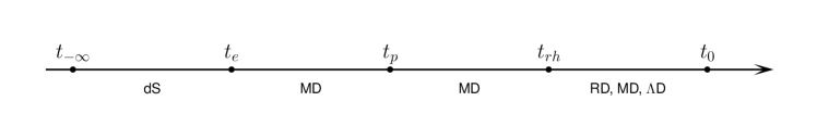
Figure 8: Thermal history of our model. Here $t_{-\infty}$ represents the initial time in our simulation. $t_{e}$ represents the time when inflation has ended and inflaton starts to oscillates around its minimum. $t_{p}$ denotes the time when GPP is almost finished and $t_{\textrm{rh}}$ denotes the time when reheating is complete. We also use $t_{0}$ to denote the current time.

In this section we briefly review the thermal history of our universe and explain how we calculate the density to entropy ratio explicitly. Our simulation starts when the inflaton $\phi$ field stays in the inflation region, which we will formally denote it by $t_{-\infty}$. At $t=t_{e}$ the (Hubble) slow roll conditions are broken and $\phi$ field start to oscillate around its minimum. In this paper we consider the case where the oscillation part can be approximated by $\phi^{2}$, which means the energy density of the inflaton field red-shift as matter. This transition from de Sitter spacetime to matter dominated space also triggers the gravitational production of the super heavy dark matter. Most of the super heavy dark matter are produced at the beginning of the oscillation part, and we assume at $t=t_{p}$ this production is basically complete and its energy density also red-shifts as matter. Hence we have the following identity

$$\frac{\rho_{\chi}(t_{p})}{\rho_{\phi}(t_{p})}=\frac{\rho_{\chi}(t_{\textrm{rh}})}{\rho_{\phi}(t_{\textrm{rh}})}=\frac{\rho_{\chi}(t_{\textrm{rh}})}{\rho_{r}(t_{\textrm{rh}})},$$ (38)

where we have used that dark matter $\chi$ field redshifts in the same way as the inflaton $\phi$ field, and we define the reheating temperature when $\rho_{\phi}(t_{\textrm{rh}})=\rho_{r}(t_{\textrm{rh}})$. Here $\rho_{r}$ denotes the energy density in radiation. After the reheating is complete, we have

$$\frac{\rho_{\chi}(t_{\textrm{rh}})}{\rho_{r}(t_{\textrm{rh}})}=\frac{\rho_{\chi}(t_{0})}{\rho_{r}(t_{0})}\frac{T_{0}}{T_{\textrm{rh}}}.$$ (39)

The entropy density and energy density in today’s Universe reads

$$\begin{split}s_{0}&=g_{*}\frac{2\pi^{2}}{45}T_{0}^{3},\\ \rho_{r,0}&=g_{*}\frac{\pi^{2}}{30}T_{0}^{4}.\end{split}$$ (40)

Hence, we can rewrite $\rho_{r,0}=\frac{3}{4}sT_{0}$ and the energy density to entropy density reads

$$\frac{\rho_{\chi}(t_{0})}{s_{0}}=\frac{3}{4}T_{0}\frac{\rho_{\chi}(t_{0})}{\rho_{r}(t_{0})}=\frac{3m_{\chi}T_{\textrm{rh}}}{4}\frac{n_{\chi}(t_{p})}{\rho_{\phi}(t_{p})},$$ (41)

where we have used $\rho=mn$ for non-relativistic particles (CDM). The energy density of $\rho_{\phi}(t_{p})$ can be connected to the energy density of inflaton at the end of inflation

$$\rho_{\phi}(t_{p})=\rho_{\phi}(t_{e})\left(\frac{a({t_{e}})}{a(t_{p})}\right)^{3}=3m_{\text{pl}}^{2}H^{2}(t_{e})\left(\frac{a({t_{e}})}{a(t_{p})}\right)^{3}.$$ (42)

The finial expression reads

$$\frac{\rho_{\chi}(t_{0})}{s_{0}}=\frac{m_{\chi}T_{\textrm{rh}}H(t_{e})}{4m_{\text{pl}}^{2}}\left(\frac{a^{3}(t_{p})n_{\chi}(t_{p})}{a^{3}({t_{e}})H^{3}(t_{e})}\right).$$ (43)

Current observation suggests this quantity should be equal to $4\text{\cdot}{10}^{-10}\text{\,}\mathrm{GeV}$ to contribute the full amount of dark matter.

- (1) Planck collaboration, Planck 2018 results. VI. Cosmological parameters, Astron. Astrophys. 641 (2020) A6 [1807.06209].
- (2) A.D. Linde, A New Inflationary Universe Scenario: A Possible Solution of the Horizon, Flatness, Homogeneity, Isotropy and Primordial Monopole Problems, Phys. Lett. B 108 (1982) 389.
- (3) A. Albrecht and P.J. Steinhardt, Cosmology for Grand Unified Theories with Radiatively Induced Symmetry Breaking, Phys. Rev. Lett. 48 (1982) 1220.
- (4) D.H. Lyth and D. Roberts, Cosmological consequences of particle creation during inflation, Phys. Rev. D 57 (1998) 7120 [hep-ph/9609441].
- (5) D.J.H. Chung, E.W. Kolb and A. Riotto, Superheavy dark matter, Phys. Rev. D 59 (1998) 023501 [hep-ph/9802238].
- (6) E.W. Kolb and A.J. Long, Cosmological gravitational particle production and its implications for cosmological relics, 2312.09042.
- (7) D.J.H. Chung, E.W. Kolb and A. Riotto, Nonthermal supermassive dark matter, Phys. Rev. Lett. 81 (1998) 4048 [hep-ph/9805473].
- (8) E.W. Kolb, D.J.H. Chung and A. Riotto, WIMPzillas!, AIP Conf. Proc. 484 (1999) 91 [hep-ph/9810361].
- (9) V. Mukhanov, Physical Foundations of Cosmology, Cambridge University Press, Oxford (2005), 10.1017/CBO9780511790553.
- (10) S. Ling and A.J. Long, Superheavy scalar dark matter from gravitational particle production in -attractor models of inflation, Phys. Rev. D 103 (2021) 103532 [2101.11621].
- (11) M.A.G. Garcia, M. Pierre and S. Verner, New window into gravitationally produced scalar dark matter, Phys. Rev. D 108 (2023) 115024 [2305.14446].
- (12) V. Kuzmin and I. Tkachev, Matter creation via vacuum fluctuations in the early universe and observed ultrahigh-energy cosmic ray events, Phys. Rev. D 59 (1999) 123006 [hep-ph/9809547].
- (13) D.J.H. Chung, L.L. Everett, H. Yoo and P. Zhou, Gravitational Fermion Production in Inflationary Cosmology, Phys. Lett. B 712 (2012) 147 [1109.2524].
- (14) P.W. Graham, J. Mardon and S. Rajendran, Vector Dark Matter from Inflationary Fluctuations, Phys. Rev. D 93 (2016) 103520 [1504.02102].
- (15) A. Ahmed, B. Grzadkowski and A. Socha, Gravitational production of vector dark matter, JHEP 08 (2020) 059 [2005.01766].
- (16) E.W. Kolb and A.J. Long, Completely dark photons from gravitational particle production during the inflationary era, JHEP 03 (2021) 283 [2009.03828].
- (17) M. Gorghetto, E. Hardy, J. March-Russell, N. Song and S.M. West, Dark photon stars: formation and role as dark matter substructure, JCAP 08 (2022) 018 [2203.10100].
- (18) J.A.R. Cembranos, L.J. Garay, A. Parra-López and J.M. Sánchez Velázquez, Vector dark matter production during inflation and reheating, JCAP 02 (2024) 013 [2310.07515].
- (19) O. Özsoy and G. Tasinato, Vector dark matter, inflation, and non-minimal couplings with gravity, JCAP 06 (2024) 003 [2310.03862].
- (20) F. Hasegawa, K. Mukaida, K. Nakayama, T. Terada and Y. Yamada, Gravitino Problem in Minimal Supergravity Inflation, Phys. Lett. B 767 (2017) 392 [1701.03106].
- (21) R. Kallosh, L. Kofman, A.D. Linde and A. Van Proeyen, Gravitino production after inflation, Phys. Rev. D 61 (2000) 103503 [hep-th/9907124].
- (22) I. Antoniadis, K. Benakli and W. Ke, Salvage of too slow gravitinos, JHEP 11 (2021) 063 [2105.03784].
- (23) K. Kaneta, W. Ke, Y. Mambrini, K.A. Olive and S. Verner, Gravitational production of spin-3/2 particles during reheating, Phys. Rev. D 108 (2023) 115027 [2309.15146].
- (24) G. Casagrande, E. Dudas and M. Peloso, On energy and particle production in cosmology: the particular case of the gravitino, JHEP 06 (2024) 003 [2310.14964].
- (25) E.W. Kolb, S. Ling, A.J. Long and R.A. Rosen, Cosmological gravitational particle production of massive spin-2 particles, JHEP 05 (2023) 181 [2302.04390].
- (26) H.P. Nilles, M. Peloso and L. Sorbo, Nonthermal production of gravitinos and inflatinos, Phys. Rev. Lett. 87 (2001) 051302 [hep-ph/0102264].
- (27) H.P. Nilles, M. Peloso and L. Sorbo, Coupled fields in external background with application to nonthermal production of gravitinos, JHEP 04 (2001) 004 [hep-th/0103202].
- (28) D.J.H. Chung, Classical Inflation Field Induced Creation of Superheavy Dark Matter, Phys. Rev. D 67 (2003) 083514 [hep-ph/9809489].
- (29) Y. Ema, K. Nakayama and Y. Tang, Production of Purely Gravitational Dark Matter, JHEP 09 (2018) 135 [1804.07471].
- (30) J.A.R. Cembranos, L.J. Garay and J.M. Sánchez Velázquez, Gravitational production of scalar dark matter, JHEP 06 (2020) 084 [1910.13937].
- (31) S. Enomoto and T. Matsuda, The exact WKB for cosmological particle production, JHEP 03 (2021) 090 [2010.14835].
- (32) E.E. Basso and D.J.H. Chung, Computation of gravitational particle production using adiabatic invariants, JHEP 11 (2021) 146 [2108.01653].
- (33) S. Hashiba and Y. Yamada, Stokes phenomenon and gravitational particle production — How to evaluate it in practice, JCAP 05 (2021) 022 [2101.07634].
- (34) E. Basso, D.J.H. Chung, E.W. Kolb and A.J. Long, Quantum interference in gravitational particle production, JHEP 12 (2022) 108 [2209.01713].
- (35) K. Kaneta, S.M. Lee and K.-y. Oda, Boltzmann or Bogoliubov? Approaches compared in gravitational particle production, JCAP 09 (2022) 018 [2206.10929].
- (36) D. Racco, S. Verner and W. Xue, Gravitational production of heavy particles during and after inflation, JHEP 09 (2024) 129 [2405.13883].
- (37) S. Verner, Nonminimal Superheavy Dark Matter, 2408.11889.
- (38) L. Jenks, E.W. Kolb and K. Thyme, Gravitational Particle Production of Scalars: Analytic and Numerical Approaches Including Early Reheating, 2410.03938.
- (39) T. Markkanen and S. Nurmi, Dark matter from gravitational particle production at reheating, JCAP 02 (2017) 008 [1512.07288].
- (40) M. Fairbairn, K. Kainulainen, T. Markkanen and S. Nurmi, Despicable Dark Relics: generated by gravity with unconstrained masses, JCAP 04 (2019) 005 [1808.08236].
- (41) S. Clery, Y. Mambrini, K.A. Olive, A. Shkerin and S. Verner, Gravitational portals with nonminimal couplings, Phys. Rev. D 105 (2022) 095042 [2203.02004].
- (42) Z. Yu, C. Fu and Z.-K. Guo, Particle production during inflation with a nonminimally coupled spectator scalar field, Phys. Rev. D 108 (2023) 123509 [2307.03120].
- (43) M.A.G. Garcia, M. Pierre and S. Verner, Scalar dark matter production from preheating and structure formation constraints, Phys. Rev. D 107 (2023) 043530 [2206.08940].
- (44) M.A.G. Garcia, M. Pierre and S. Verner, Isocurvature constraints on scalar dark matter production from the inflaton, Phys. Rev. D 107 (2023) 123508 [2303.07359].
- (45) M. Endo, M. Kawasaki, F. Takahashi and T.T. Yanagida, Inflaton decay through supergravity effects, Phys. Lett. B 642 (2006) 518 [hep-ph/0607170].
- (46) M. Endo, F. Takahashi and T.T. Yanagida, Spontaneous Non-thermal Leptogenesis in High-scale Inflation Models, Phys. Rev. D 74 (2006) 123523 [hep-ph/0611055].
- (47) M. Endo, F. Takahashi and T.T. Yanagida, Inflaton Decay in Supergravity, Phys. Rev. D 76 (2007) 083509 [0706.0986].
- (48) S. Enomoto, S. Iida, N. Maekawa and T. Matsuda, Beauty is more attractive: particle production and moduli trapping with higher dimensional interaction, JHEP 01 (2014) 141 [1310.4751].
- (49) Y. Ema, M.A.G. Garcia, W. Ke, K.A. Olive and S. Verner, Inflaton Decay in No-Scale Supergravity and Starobinsky-like Models, Universe 10 (2024) 239 [2404.14545].
- (50) K. Nakayama, A Note on Gravitational Particle Production in Supergravity, Phys. Lett. B 797 (2019) 134857 [1905.09143].
- (51) E.J. Copeland, A.R. Liddle, D.H. Lyth, E.D. Stewart and D. Wands, False vacuum inflation with Einstein gravity, Phys. Rev. D 49 (1994) 6410 [astro-ph/9401011].
- (52) G. Dall’Agata and F. Zwirner, On sgoldstino-less supergravity models of inflation, JHEP 12 (2014) 172 [1411.2605].
- (53) R. Kallosh, A. Linde and M. Scalisi, Inflation, de Sitter Landscape and Super-Higgs effect, JHEP 03 (2015) 111 [1411.5671].
- (54) R. Kallosh, A. Linde and D. Roest, Superconformal Inflationary -Attractors, JHEP 11 (2013) 198 [1311.0472].
- (55) G. Germán, On the -attractor t-models, Journal of Cosmology and Astroparticle Physics 2021 (2021) 017.
- (56) Planck collaboration, Planck 2018 results. X. Constraints on inflation, Astron. Astrophys. 641 (2020) A10 [1807.06211].
- (57) D.J.H. Chung, E.W. Kolb, A. Riotto and L. Senatore, Isocurvature constraints on gravitationally produced superheavy dark matter, Physical Review D 72 (2005) .
- (58) R. Kallosh, A. Linde and T. Rube, General inflaton potentials in supergravity, Phys. Rev. D 83 (2011) 043507 [1011.5945].
- (59) E.W. Kolb, A.J. Long, E. McDonough and G. Payeur, Completely dark matter from rapid-turn multifield inflation, Journal of High Energy Physics 2023 (2023) .
- (60) K.D. Lozanov and M.A. Amin, Self-resonance after inflation: Oscillons, transients and radiation domination, Physical Review D 97 (2018) 023533 [1710.06851].
- (61) M.A. Amin, M.P. Hertzberg, D.I. Kaiser and J. Karouby, Nonperturbative Dynamics Of Reheating After Inflation: A Review, International Journal of Modern Physics D 24 (2015) 1530003 [1410.3808].
- (62) B. Barman, S. Cléry, R.T. Co, Y. Mambrini and K.A. Olive, Gravity as a portal to reheating, leptogenesis and dark matter, Journal of High Energy Physics 2022 (2022) .
- (63) M.M. Flores and Y.F. Perez-Gonzalez, On the role of cosmological gravitational particle production in baryogenesis, 2024.
- (64) J.D. Hunter, Matplotlib: A 2D graphics environment, Computing in Science & Engineering 9 (2007) 90.
- (65) P. Virtanen, R. Gommers, T.E. Oliphant, M. Haberland, T. Reddy, D. Cournapeau et al., SciPy 1.0: Fundamental algorithms for scientific computing in python, Nature Methods 17 (2020) 261.
- (66) C.R. Harris, K.J. Millman, S.J. van der Walt, R. Gommers, P. Virtanen, D. Cournapeau et al., Array programming with NumPy, Nature 585 (2020) 357.
- (67) C. Rackauckas and Q. Nie, DifferentialEquations.jl–a performant and feature-rich ecosystem for solving differential equations in Julia, Journal of Open Research Software 5 (2017) .