Rough or crumpled: Strong coupling phases of a generalized Kardar-Parisi-Zhang surface

Abstract

We study a generalized Kardar-Parisi-Zhang (KPZ) equation [D. Jana et al, Phys. Rev. E 109, L032104 (2024)], that sets the paradigm for universality in roughening of growing nonequilibrium surfaces without any conservation laws, but with competing local and nonlocal nonlinear effects. We show that such a generalized KPZ equation in two dimensions can describe a strong coupling rough or a crumpled surface, in addition to a weak coupling phase. The conformation fluctuations of such a rough surface are given by nonuniversal exponents, with orientational long-ranged order and positional short-ranged order, whereas the crumpled phase has positional and orientational short range order. Experimental and theoretical implications of these results are discussed.

The Kardar-Parisi-Zhang (KPZ) equation Kardar et al. (1986); Krug (1997); Barabási and Stanley (1995), originally proposed as a model for growing surfaces without overhangs, provides a paradigm for nonequilibrium phase transitions. It undergoes a roughening transition between a smooth phase, statistically identical to a surface described by the linear Edwards-Wilkinson (EW) equation Edwards and Wilkinson (1982), and a perturbatively inaccessible strong coupling phase Barabási and Stanley (1995), in dimension $d>2$. Perturbative dynamic renormalization group (RG) Barabási and Stanley (1995); Täuber (2014) analysis has been successful in describing this roughening transition in an $\epsilon$-expansion, where $d=2+\epsilon$, with two dimensions (2D) being the lower critical dimension of the model. In $d\leq 2$, there exists only the strong coupling phase. A KPZ surface described by a single-valued height field $h({\bf x},t)$ measured with respect to an arbitrary base plane in the Monge gauge Nelson et al. (1989) displays universal scaling in the long wavelength limit, characterized by $z$ and $\chi$, the dynamic and roughness exponents Barabási and Stanley (1995). These are formally defined through the correlation function

$$C(r,t)\equiv\langle[h({\bf x},t)-h({\bf 0},0)]^{2}\rangle\sim r^{2\chi}\phi({r^{z}}/{t})$$ (1)

in the scaling limit, where $r=|{\bf x}|$ and $\phi$ is a dimensionless scaling function of its argument Barabási and Stanley (1995). In the smooth phase, $z=2$ and $\chi=1-d/2$ Barabási and Stanley (1995) and at the roughening transition at $d=2+\epsilon,\,\epsilon>0$, $z=2$ and $\chi=0$ Barabási and Stanley (1995); Täuber (2014); Janssen et al. (1999). Failure of RG to capture the strong coupling phase has led to the development of alternative techniques. Notable are the self-consistent mode-coupling theories (MCT) Bouchaud and Cates (1993); Bhattacharjee (1998), which have predicted a variety of results on scaling within specific different calculational approaches. For example Ref. Hwa and Frey (1991) explored the scenario with $d=1$, yielding $z=3/2$, a value known exactly due to the Galilean invariance and a Fluctuation-Dissipation-Theorem Barabási and Stanley (1995). Furthermore, Ref. Doherty et al. (1994) shows that $z$ rises from $z=3/2$ at $d=1$ to 2 around $d_{U}=3.6$, the upper critical dimension of the KPZ equation. In contrast, Ref. Tu (1994) suggests $z<2$ at any finite dimension indicating $d_{U}=\infty$. Furthermore, Refs. Bhattacharjee (1998); Bhattacharjee and Bhattacharyya (2007); Basu and Frey (2004, 2009a) used MCT to predict $\chi=(4-d)/6,\,z=(8+d)/6$ that tend to agree reasonably with the numerical results Gomes-Filho et al. (2021). See also Ref. Colaiori and Moore (2001), which gives $d_{c}=4$ and dynamic exponent $z$ in different dimensions. More recently, Ref. Canet and Moore (2007) revisited the MCT for the KPZ equation and showed that solutions for the MCT equations for the KPZ equation actually have two branches or two distinct universality classes below $d<2$. At $d\geq 2$, there is only one branch that continues to $d_{U}=4$, giving scaling exponents closed to those known from numerical studies.

The dynamics of a KPZ surface depends locally on surface fluctuations, and hence cannot model nonequilibrium surfaces with nonlocal dynamics. Nonlocal effects, however, can be important in wide-ranging systems, including biological growth process Santalla and Ferreira (2018), fast nonlocal transport Aharonov and Rothman (1996) and nonlocal stabiliztion of surfaces Krug and Meakin (1991); Nicoli et al. (2009). Recently, a generalized or “active” KPZ equation (hereafter a-KPZ equation) with nonlocal effects as a conceptual model with competing local and nonlocal nonlinear effects has been proposed Jana et al. (2024)

$$\frac{\partial h}{\partial t} = \nu\nabla^{2}h+\frac{\lambda}{2}(\bm{\nabla}h)^{2}$$ (2)

$$+ \lambda_{1}\int d^{d}rQ_{ij}({\bf r-r^{\prime}})(\nabla_{i}h({\bf r^{\prime}},t)\nabla_{j}h({\bf r^{\prime}},t))+\eta.$$

Here, $Q_{ij}({\bf r})$ denotes the longitudinal projection operator, which in Fourier space is expressed as $Q_{ij}({\bf k})=k_{i}k_{j}/k^{2}$, with ${\bf k}$ being a Fourier wave vector. Thus $Q_{ij}({\bf r})$, which is the inverse Fourier transform of $Q_{ij}({\bf k})$, is nonlocal in space. Physically, the term $\lambda_{1}\int d^{d}rQ_{ij}({\bf r-r^{\prime}})(\nabla_{i}h({\bf r^{\prime}},t)\nabla_{j}h({\bf r^{\prime}},t))$ contributes to the surface velocity normal to the base plane, $v_{p}=\partial h/\partial t$, and is nonlocal in ${\bm{\nabla}}h$. Furthermore, $\eta({\bf x},t)$ is a zero-mean Gaussian-distributed white noise with a variance $\langle\eta({\bf x},t)\eta({\bf 0},0)\rangle=2D\delta^{d}({\bf x})\delta(t).$ If $\lambda_{1}=0$, Eq. (2) reduces to the usual KPZ equation. As a consequence of the competition between the local and nonlocal nonlinearities, a-KPZ equation (2) shows macroscopic properties dramatically different from the KPZ equation. It can have a stable, sub- or super-logarithmically rough surface in 2D, characterized by nonuniversal scaling exponents. More strikingly and unlike the 2D KPZ equation, it also admits a roughening transition even in 2D, again characterized by nonuniversal exponents. At $d>2$, it shows a roughening transition different from that in the KPZ equation Jana et al. (2024). Equation (2) admits a pseudo-Galilean invariance under the transformation $x_{i}^{\prime}=x_{i}-(\lambda+2\lambda_{1})c_{i}t$ and $t^{\prime}=t$, together with $h^{\prime}({\bf x}^{\prime},t^{\prime})=h({\bf x},t)+\textbf{c}\cdot\textbf{x}$, which ensures that the combination $\lambda+2\lambda_{1}$ does not renormalize; see also Ref. Jana et al. (2024). This further means $\chi+z=2$ exactly so long as nonlinearities remain relevant (in the scaling sense).

In this Letter, we focus on the strong coupling phases of (2). We show that these strong coupling phases can be of two distinct kinds: (i) rough phase with positional short range order (SRO), but orientational long range order (LRO), or (ii) crumpled with both positional and orientational SRO. We extract the scaling exponents of the rough phase in $d\geq 2$, which show their nonuniversal nature: The variance $\Delta\equiv\langle[h({\bf x},t)-\overline{h}(t)]^{2}\rangle\sim L^{2\chi(\gamma)}$, $0<\chi(\gamma)<1$ where $L$ is the linear size of the surface and $\overline{h}(t)$ is the average height at time $t$. Furthermore, the time-scale of relaxation $\tau(L)\sim L^{z(\gamma)}$. Both $\chi$ and $z$ are parametrized continuously by $\gamma\equiv\lambda_{1}/\lambda$, reflecting model parameter-dependent, nonuniversal scaling. In the crumpled phase, $\chi>1$.

We now derive the above results. Nonlinear terms preclude any exact analysis. We first use a Wilson dynamic RG framework Kardar et al. (1986); Barabási and Stanley (1995); Forster et al. (1977); Täuber (2014) and build upon the results discussed in Ref. Jana et al. (2024). Dimensional analysis allows us to define two effective dimensionless coupling constants:

$$g\equiv\frac{\lambda^{2}D}{\nu^{3}}k_{d},\,g_{1}\equiv\frac{\lambda_{1}^{2}D}{\nu^{3}}k_{d},\,g_{2}\equiv\text{sign}(\gamma)\sqrt{g_{1}}.$$ (3)

Here $k_{d}=\frac{S_{d}}{(2\pi)^{d}}$, and $S_{d}$ is the surface area of a $d$-dimensional sphere. Considering $\lambda>0$ without any loss of generality, we notice that from (3) above that $g_{2}$ can be both positive and negative, depending upon the sign of $\gamma$. There are no one-loop corrections to $\lambda,\lambda_{1}$. The one-loop corrections to $\nu$ and $D$ can be obtained following Refs. Barabási and Stanley (1995); Forster et al. (1977); Jana et al. (2024), which allow us to calculate the one-loop RG flow equations for $g$, $g_{1}$ and hence $g_{2}$,

$$\frac{dg}{dl} = g[2-d-g\tilde{A}(\gamma)],$$ (4)

$$\frac{dg_{2}}{dl} = \frac{g_{2}}{2}[2-d-g\tilde{A}(\gamma)],$$ (5)

where $\tilde{A}(\gamma)=\frac{9}{8}\gamma^{2}+\frac{11}{8}\gamma-\frac{1}{4}$. Considering 2D, the physically relevant dimension, we focus on the RG flow lines in the $g$-$g_{2}$ plane, with (0,0) as the only RG fixed point. Its stability properties are intriguing. It is stable (i.e., attractive) along the $g_{2}$-axis, but unstable (i.e., repulsive) along the $g$-axis. This indicates the existence of a separatrix, an invariant manifold under RG in the $g$-$g_{2}$ plane, that separates the stable phase from instability. While (0,0) is the only fixed point of both (22) and (23), it may be stable or unstable. Stability requires $dg/dl<0,dg_{2}/dl<0$, so that both $g(l),\,g_{2}(l)$ flow to zero in the long wavelength limit. Else when $dg/dl>0,dg_{2}/dl>0$, both $g(l),\,g_{2}(l)$ flow away from (0,0) giving instability. These two behaviors are demarcated by the separatrices $\tilde{A}(\gamma)=0$, giving

$$g_{2}=(0.161)\sqrt{g},\;g_{2}=-1.383\sqrt{g}$$ (6)

for $\lambda_{1}>0$ and $\lambda_{1}<0$, respectively, as the separatrices, in $g$-$g_{2}$ plane passing through (0,0). The RG flow diagram in 2D is shown in Fig. 1(a). The red lines in Fig. 1(a) are the separatrices given in (6): the RG flow lines in the green regions bordered by the separatrices flow to the origin, giving the “weak coupling phase”. Although (0,0) is the stable fixed point in this region, the flow to (0,0) is so slow that $\nu$ and $D$ are infinitely renormalized, giving being super- or sub-logarithmically rough phases, as explored in Ref. Jana et al. (2024). In the remaining regions, both $g$ and $g_{2}$ grow monotonically with the “RG time” $l$. As soon as $g(l),\,g_{2}(l)\sim{\cal O}(1)$, which happens for a surface of finite size, the RG flow equations are outside the validity of the perturbative expansions. This is the perturbatively inaccessible “strong coupling phase”.

We first argue that the region confined between the two separatrices [red lines in Fig. 1(a)] actually consists of two subregions with distinct scaling properties (instead of just one region with a rough phase, as originally speculated in Ref. Jana et al. (2024)). To investigate that let us first consider the bare perturbation theory for $\nu$ in 2D, which is same as the RG calculations for $\nu$ except that now we extend the integrals over wave vectors down to an infrared cutoff $q_{\text{min}}=2\pi/L$. Setting $d=2$, we get for the effective $\nu_{e}$

$$\nu_{e}\approx\nu_{0}+g\nu_{0}\Bigl{(}\frac{1}{2}\gamma^{2}+\frac{5}{8}\gamma\Bigl{)}\ln(L/a).$$ (7)

We thus find that for $\Bigl{(}\frac{1}{2}\gamma^{2}+\frac{5}{8}\gamma\Bigl{)}<0$ or $\Bigl{(}\frac{(g_{2})^{2}}{2g}+\frac{5g_{2}}{8\sqrt{g}}\Bigl{)}<0$ i.e. $-1.25<\gamma<0$, $\nu_{e}<\nu_{0}$. In fact, for sufficiently large $L/a$, $\nu_{e}<0$, giving divergence of $\langle({\bm{\nabla}}h)^{2}\rangle$ implying surface crumpling with positional and orientational SRO. In higher dimensions $d>2$, the one loop integrals are finite and hence the lower limit can be extended to 0, corresponding to the thermodynamic limit. Then for a range of $\gamma$, $-1.25<\gamma<0$ and low enough bare $\nu_{0}$, $\nu_{e}$ can turn negative, once again implying crumpling. We will revisit the region with crumpling below, shown in purple in Fig. 1(a), by using mode coupling methods, and come to a similar conclusion, giving us confidence about the existence of a crumpled phase. See Fig. 1(b) for a schematic phase diagram in the $\lambda-\lambda_{1}$ plane.

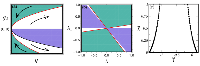
Figure 1: (a) RG flow diagram in the $g$-$g_{2}$ plane in 2D. Stable and unstable regions are divided by the separatrices (red lines). Stable (Unstable) regions are indicated by flow lines moving towards (away from) the origin. The arrows indicate the flow directions, delineating the stable and unstable regions. In this flow diagram (0,0) is the only fixed point that is unstable along the $g$-direction, but stable along the $g_{2}$-direction. (b) Phases in the $\lambda-\lambda_{1}$ plane. The green regions are the weak coupling logarithmically rough phase, the white regions are the algebraically rough phase, and the purple regions are the crumpled phase. In (a) and (b) the solid red line represents the locus of unstable fixed points where the roughening transition occurs. (c) Variation of $\chi$ in 2D in the phase space region where it is positive, with $\gamma$ as obtained from MCT. Central region where $\chi>1$, corresponds to a crumpled surface.

To study the unstable regions in the RG flow diagrams, we now set up an MCT calculation Bhattacharjee (1998); Basu and Frey (2009b) to extract the scaling behavior; see also Basu (2004); Basu and Bhattacharjee (2005) for applications of MCT in a slightly different context. The response $G({\bf k},\omega)$ and correlation $C({\bf k},\omega)$ functions have the following scaling form

$$G({\bf k},\omega)=k^{-z}g\biggl{(}\frac{\omega}{k^{z}}\biggr{)}=-i\omega+\Sigma(k,\omega),$$ (8)

$$C({\bf k},\omega)=k^{-d-2\chi-z}f\biggl{(}\frac{\omega}{k^{z}}\biggr{)}.$$ (9)

where the self-energy $\Sigma({\bf k},\omega=0)=\Gamma k^{z}$ in the zero frequency limit. Similarly for the correlator in the Lorentzian approximation, we write

$$C({\bf k},\omega)=\frac{2D\Gamma k^{-2\chi-d+z}}{\omega^{2}+\Gamma^{2}k^{2z}}.$$ (10)

Our argument is that the universal amplitude ratio $\Gamma^{2}/(D\lambda^{2})$ can be written down both from the one-loop diagrammatics of $G^{-1}({\bf k},\omega)$ and $C({\bf k},\omega)$. We use $\chi+z=2$, which is an exact result in the strong coupling phases (also consistent with the absence of vertex corrections at the one-loop order). Further assuming that $G^{-1}$ and $C$ are dominated by their respective one-loop contributions,which would hold if $z<2$ and $\chi>0$. Combining contributions from all the one-loop diagrams for $G({\bf k},\omega=0)$, we obtain sup

$$\frac{\Gamma^{2}}{\lambda^{2}D}=\frac{k_{d}}{\chi\,d}\biggl{[}\frac{\chi}{2}+\gamma\biggl{(}\frac{4d+2d^{2}+2\chi d+10\chi-6}{2(d+2)}\biggl{)}$$

$$\quad\quad\quad\quad\quad\quad\quad\quad\quad\quad\quad\quad+\gamma^{2}\biggl{(}\frac{6\chi+4d-4}{d+2}\biggl{)}\biggl{]}.$$ (11)

Next, considering the one-loop contributions to $C({\bf k},\omega=0)$, we find

$$\frac{\Gamma^{2}}{\lambda^{2}D}=\frac{k_{d}\biggl{[}d(d+2)+4\gamma(d+2)+12\gamma^{2}\biggl{]}}{4d(d+2)(d+3\chi-2)}.$$ (12)

Now comparing RHS of Eqs. (58) and (71), we obtain a quadratic equation of $\chi$

$$A\chi^{2}+B\chi+C=0.$$ (13)

Here, $A=36\gamma^{2}+(6d+30)\gamma+(3d+6),\,B=(36d-54)\gamma^{2}+(8d^{2}+16d-42)\gamma+\biggl{(}\frac{d^{2}}{2}-4-d\biggl{)},\,C=(d-2)\gamma\bigl{[}\gamma(8d-8)+(2d^{2}+4d-6)\bigl{]}.$ Solving (13)

$$\chi=\frac{-B\pm|\sqrt{B^{2}-4AC}|}{2A}=\chi_{\pm}.$$ (14)

We take $\chi=\chi_{+}$, for $\gamma=0$ only $\chi_{+}$ reduces to $\chi=1/2$ at $d=1$, the known exact value; incidentally, the choice $\chi=\chi_{+}$ reduces to $\chi=1/3$ in 2D obtained in an analogous MCT for the pure KPZ equation along with $d_{U}=4$ Bhattacharjee (1998) for $\gamma=0$. We now calculate $\chi$ in 2D. By setting $d=2$ in $A$, $B$ and $C$ defined above, we get $C=0$ and $\chi=\frac{-B+|B|}{2A}$ where, $B=18\gamma^{2}+22\gamma-4$ and $A=36\gamma^{2}+42\gamma+12$. Validity of our MCT requires $\chi>0$. This means either $B<0$ and $A>0$, or $B>0$ and $A<0$. Notice that $B=0$ gives the separatrix (6) with $B<0$ corresponds to the unstable region in Fig. 1(a). We focus on the region $B<0$, which holds for $-1.383<\gamma<.161$. Within this region,

$$\chi=\frac{-B}{A}=\frac{-18\gamma^{2}-22\gamma+4}{36\gamma^{2}+42\gamma+12}.$$ (15)

On the separatrices (6), $B=0$ and $A=22.77$ corresponding to $\gamma=\gamma_{c1}=0.161$ and $A=19.69$ corresponding to $\gamma=\gamma_{c2}=-1.383$; $A$ changes from these boundary values within the unstable region between the separatrices. In particular, as $A$, depending upon $\gamma$, decreases, $\chi$ grows, eventually exceeding unity. At this point, our theory (2) breaks down, as $\langle({\bm{\nabla}}h)^{2}\rangle$ diverges with $L$, giving a crumpled surface. (We make a technical point here that as $\chi$ exceeds unity, higher order nonlinear terms not included in (2) become relevant (in a RG sense), making our theory given by Eq. (2) to breakdown.) Setting $\chi=1$ in (15), we get $\gamma=-1.043,-0.142$. Thus in the region $(-1.043<\gamma<-0.142)$ MCT predicts existence of a crumpled phase, which is the purple region in Fig. 1(a) and is slightly different from the region defined by $\nu_{e}=0$ (see above). Due to the breakdown of our theory, we cannot make any definitive conclusion about any scaling properties in the crumpled region.

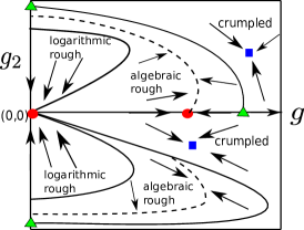
Figure 2: Conjectured “Occam’s razor” global RG flows in the $g$-$g_{2}$ plane. Different speculated fixed points characterizing the rough and crumpled phases are marked. The broken lines are speculated fixed lines in the rough phase; see text.

We now focus on the region where $0<\chi<1$. When $B=0$, which gives the separatrices (6), we have $\chi=0$, giving two solutions for $\gamma=-1.383,\,0.161$. These are the red lines in Fig. 1(a). Within the region demarcated by $0<\chi<1$, $\chi$ follows Eq. (15) which is parametrized by $\gamma$. Thus we have nonuniversal scaling exponents, that has its origin in the competition between the nonlocal and local nonlinearities in (2). The variation of $\chi$ with $\gamma$ is depicted in Fig. 1(c). In a renormalization group language, this nonuniversality in scaling indicates a fixed line, as opposed to a fixed point, that characterizes the rough phase. Such nonuniversal $\chi(\gamma)$ are reminiscent of the analogous nonuniversal exponents found in the logarithmically rough phase in Ref. Jana et al. (2024). The vanishing of $\chi$ at $\gamma=\gamma_{c2}=-1.383$ and $\gamma=\gamma_{c1}=0.161$ defines the boundary between regions with logarithmically rough and algebraically rough surfaces, which exactly matches with the predictions from RG analysis Jana et al. (2024). Outside the unstable region, i.e., for $\gamma>\gamma_{c1}$ or $\gamma<\gamma_{c2}$, one has $\chi<0$, which falls outside the validity regime of our MCT. Since $\chi<0$ is predicted from (15) for $|\gamma|\rightarrow\infty$, the whole $g_{2}$ axis should fall outside the rough phase (and also of course the crumpled phase) and describe the logarithmically rough phase found in Ref. Jana et al. (2024). At $\gamma=0$ we recover the KPZ result with $\chi=1/3$ Bhattacharjee (1998).

Having ascertained the existence of rough and crumpled phases in 2D, we now speculate on the global fixed point structure including the strong coupling fixed points, which are inaccessible to perturbative RG; see Fig. 2. The RG flow lines that flow out of the fixed point (0,0) in the unstable region of the phase space should flow to one of these fixed points. To analyze these fixed points, we are first guided by the expectation that there should be a strong coupling fixed point at $g\neq 0,g_{2}=0$, which is the expected 2D KPZ string coupling fixed point and should govern the scaling laws for a 2D KPZ surface (which is rough). This is marked by a red circle (the other red circle at the origin is another fixed point that is unstable along the $g$-direction, but stable along the $g_{2}$-direction). In the present model, this fixed point is expected to be unstable against perturbation by a finite $\gamma$ or $g_{2}$. On one side of the $g$-axis, there should be a crumpled phase, which we expect to be characterized by a stable crumpled phase fixed point, marked by a blue square in Fig. 2. On the other side of the $g$-axis, there should be a rough phase. Considering the MCT prediction of nonuniversal scaling in the rough phase, we speculate a fixed line marked by broken line in Fig. 2, corresponding to the rough phase. On the side of the $g$-axis with a crumpling fixed, we also expect to have a stable rough phase fixed line for higher negative values of $g_{2}$ (or higher negative values of $\gamma$), giving nonuniversal scaling. Finally, we generally expect that for larger noises, i.e., with larger values of $D$, for which both $g$ and $g_{2}$ grow, the surface should be less and less ordered. This line of reasoning suggests that there should be a crumpling fixed point on the $g$-axis beyond the putative 2D KPZ rough phase fixed point, as well as on the $g_{2}$ axis (marked by a green triangle), indicating eventual crumpling of the surface for high enough $g$ or $g_{2}$. These are basically an “Occam”-razor style arguments: Fig. 2 has the simplest topology that naturally reduces to the known RG flow lines for small $g,\,g_{2}$, as shown in Fig. 1(a). At the same time, it gives the putative global flow lines, allowing for a transition to presumed rough and crumpled phases; see Ref. Banerjee et al. (2019); Mukherjee and Basu (2022a, b) for similar Occam’s razor arguments in different contexts.

We now consider the model in higher dimensions: $d>2$. In $d=2+\epsilon>2$, there are additional fixed points of the RG flows, other than (0,0) (stable fixed point) in the $g$-$g_{2}$ plane. In the accessible region i.e. $\tilde{A}(\gamma)>0$, (0,0) is the only stable fixed point and the long-wavelength scaling behavior matches that of the Edwards-Wilkinson (EW) equation, characterized by $z=2,\,\chi=(2-d)/2$ Jana et al. (2024). In the perturbatively inaccessible strong coupling phase, i.e., $\tilde{A}(\gamma)<0$, from an RG analysis Ref. Jana et al. (2024) argued a roughening transition with an associated $\chi=-\epsilon\,\tilde{C}(\gamma)/{\tilde{A}(\gamma)}$; $\tilde{C}(\gamma)\equiv\gamma^{2}/2+5\gamma/8$. For any $\epsilon>0$, at the roughening transition $\chi$ can grow arbitrarily large, if $\tilde{A}(\gamma)$ becomes small enough (remaining negative). As $\chi$ exceeds unity, our theory (2) breaks down, as $\langle({\bm{\nabla}}h)^{2}\rangle$ diverges with $L$, giving a crumpled surface. (We make a technical point here that as $\chi$ exceeds unity, higher order nonlinear terms not included in (2) become relevant (in a RG sense), making our theory given by Eq. (2) to breakdown.) Setting $\chi=1$, we get a limit on $\gamma$, up to which this roughening transition between a smooth phase and an algebraically rough phase can be observed. Beyond this threshold value of $\gamma$ there is a range of $\gamma$ bounded by another threshold such that in the entire range $\tilde{A}(\gamma)$ is small enough to make $\chi>1$, suggesting that the roughening transition in this range of $\gamma$ is actually between a smooth phase and a crumpled phase (and not a rough phase)! Overall thus, similar to our discussions for 2D, we expect the strong coupling phase to consist of a rough phase with $0<\chi<1$ and a crumpled phase with $\chi>1$. Our further theoretical analysis below substantiate this expectation.

We now briefly discuss the MCT predictions for $d>2$. Our RG calculations already predicted a smooth phase and a roughening transition presumably to a strong coupling phase. The latter however cannot be accessed in the RG calculations. Assuming $\chi>0$, we apply MCT to extract the scaling behaviour in the strong coupling phase. Focusing on $d=3$, we get $A=36\gamma^{2}+48\gamma+15$, $B=54\gamma^{2}+78\gamma-2.5$ and $C=16\gamma^{2}+24\gamma$, giving $\chi\equiv\chi(\gamma)$. Thus, both $\chi$ and $z=2-\chi$ are nonuniversal, as they are in 2D. Secondly, by varying $\gamma$, one can make $\chi$ bigger, eventually exceeding unity. As in 2D, $\chi>1$ should imply crumpling of the surface, for which our theory breaks down. We therefore find that the strong coupling phase in 3D is similar to 2D. Similar analysis indicates analogous behavior in the strong coupling phase for any $d>2$.

We have thus studied the strong coupling phases of a generalized KPZ equation, in which local and nonlocal nonlinear effects compete (in the scaling sense). Our results from the RG and bare perturbation theory in 2D suggest that the strong coupling region in the parameter space the strong coupling phase actually is made of two distinct phases, one an algebraically rough phase with $0<\chi<1$ corresponding to orientational LRO but positional SRO, and another with $\chi>1$ implying a crumpled phase having both positional and orientational SRO. These are corroborated by our one-loop MCT calculations. While the crumpled phase cannot be systematically explored by our theory, our MCT predicts that the algebraic rough phase is characterized by nonuniversal scaling exponents parametrized by $\gamma$, similar to the nonuniversal exponents in the logarithmically rough phase by the RG calculations. Similar behavior including a crumpled phase and a rough phase with nonuniversal scaling exponents are predicted by MCT in 3D. The results in Ref. Jana et al. (2024) showed that chirality has the effect of suppressing the nonlinear instabilities of the RG flow. We thus expect that chiral effects together with the nonlocality should be able to suppress the crumpling of the membrane, stabilising orientational order. We note that the nonuniversal scaling exponents are a crucial outcome of the lack of vertex renormalization in one-loop MCT. We are unable to speculate whether this result protected by any “hidden” symmetry not known at present, or a fortuitous result, or will not hold at higher order perturbation theory. Thus, it would be interesting to verify our results numerically, e.g., by using pseudo-spectral methods Basu and Frey (2009a); Basu et al. (1998), or by nonperturbative methods Canet et al. (2011a, b, 2010). Nonetheless, we expect our predictions on the existence of a crumpled phase to hold true.

Acknowledgement:- A.B. thanks the SERB, DST (India) for partial financial support through the TARE scheme [file no.: TAR/2021/000170] and Alexander von Humboldt Stiftung, Germany for partial financial support through the Research Group Linkage Programme (2024).

Appendix A Renormalization group calculations

We revisit and reanalyse the renormalization group calculations on the generalized KPZ equation (2) of the main text. We follow Jana et al. (2024). We first give the path integral over $h({\bf r},t)$ and its dynamic conjugate field $\hat{h}({\bf r},t)$ Bausch et al. (1976); Täuber (2014) that is equivalent to and constructed from Eq. (2) of the main text together with the noise variance. The generating functional corresponding to Eq. (2) of the main text is given by Bausch et al. (1976); Täuber (2014)

$$\mathcal{Z}=\int\mathcal{D}\hat{h}\mathcal{D}he^{-\mathcal{S}[\hat{h},h]},$$ (16)

where $\hat{h}$ is the dynamic conjugate field and $\mathcal{S}$ is the action functional:

$$S=-\int_{{\bf x},t}\hat{h}D\hat{h}+\int_{{\bf x},t}\hat{h}\bigg{\{}\partial_{t}h-\nu\nabla^{2}h-\frac{\lambda}{2}(\bm{\nabla}h)^{2}-\lambda_{1}\frac{\nabla_{i}\nabla_{j}}{\nabla^{2}}(\nabla_{i}h\nabla_{j}h)\bigg{\}}.$$ (17)

Using the one loop diagrams from the supplemental material of Ref. Jana et al. (2024) we obtain renormalized $D$ ($D^{<}$) and renormalized $\nu$ ($\nu^{<}$):

$$D^{<}=D\Biggr{[}1+\frac{\lambda^{2}D}{\nu^{3}}k_{d}\biggl{(}\frac{1}{4}+\gamma\frac{1}{d}+\gamma^{2}\frac{3}{d(d+2)}\biggl{)}\int_{\frac{\Lambda}{b}}^{\Lambda}\frac{d^{d}q}{q^{2}}\Biggr{]},$$ (18)

$$\nu^{<}=\nu\Biggr{[}1+\frac{\lambda^{2}D}{\nu^{3}}k_{d}\biggl{(}\frac{2-d}{4d}+\frac{\gamma}{d(d+2)}\Bigl{(}3-\frac{d+2}{2}+\frac{d(d+2)}{2}\Bigl{)}+\frac{\gamma^{2}}{d}\biggl{)}\int_{\frac{\Lambda}{b}}^{\Lambda}\frac{d^{d}q}{q^{2}}\Biggr{]}.$$ (19)

Here $k_{d}=\frac{S_{d}}{(2\pi)^{d}}$, where $S_{d}$ is the surface area of a $d$-dimensional sphere and $\gamma=\frac{\lambda_{1}}{\lambda}$ as defined in the main text. Using above equations and Setting $d=2$ in the above integrals, with $b=e^{\delta l}\approx 1+\delta l$ ($l$ is the RG time) and defining dimensionless coupling constant by $g\equiv\frac{\lambda^{2}D}{\nu^{3}}k_{d}$ as in the main text, we obtain the RG flow equations for $D$ and $\nu$:

$$\frac{dD}{dl}=D\Biggr{[}z-d-2\chi+g\biggl{(}\frac{1}{4}+\gamma\frac{1}{d}+\gamma^{2}\frac{3}{d(d+2)}\biggl{)}\Biggr{]},$$ (20)

$$\frac{d\nu}{dl}=\nu\Biggr{[}z-2+g\biggl{(}\frac{2-d}{4d}+\frac{\gamma}{d(d+2)}\Bigl{(}3-\frac{d+2}{2}+\frac{d(d+2)}{2}\Bigl{)}+\frac{\gamma^{2}}{d}\biggl{)}\Biggr{]}.$$ (21)

Also defining another dimensionless coupling constant, $g_{1}\equiv\frac{\lambda_{1}^{2}D}{\nu^{3}}k_{d},\,g_{2}\equiv\text{sign}(\gamma)\sqrt{g_{1}}$ and using above equations we can write the flow equations of $g$ and $g_{2}$:

$$\frac{dg}{dl}=g\Biggr{[}2-d+g\biggl{\{}\frac{1}{4}+\frac{3}{d(d+2)}\gamma^{2}+\frac{\gamma}{d}-\frac{3}{4}\frac{2-d}{d}-\frac{3}{d}\gamma^{2}-\frac{3\gamma}{d(d+2)}\biggl{(}3-\frac{d+2}{2}+\frac{d(d+2)}{2}\biggl{)}\biggl{\}}\Biggr{]},$$

$$\frac{dg_{2}}{dl}=\frac{g_{2}}{2}\Biggr{[}2-d+g\biggl{\{}\frac{1}{4}+\frac{3}{d(d+2)}\gamma^{2}+\frac{\gamma}{d}-\frac{3}{4}\frac{2-d}{d}-\frac{3}{d}\gamma^{2}-\frac{3\gamma}{d(d+2)}\biggl{(}3-\frac{d+2}{2}+\frac{d(d+2)}{2}\biggl{)}\biggl{\}}\Biggr{]}.$$

To the lowest order in $d-d_{c}$, where $d_{c}=2$ is the critical dimension,

$$\frac{dg}{dl} = g[2-d-g\tilde{A}(\gamma)],$$ (22)

$$\frac{dg_{2}}{dl} = \frac{g_{2}}{2}[2-d-g\tilde{A}(\gamma)].$$ (23)

Where $\tilde{A}(\gamma)=\frac{9}{8}\gamma^{2}+\frac{11}{8}\gamma-\frac{1}{4}$ as given in the main text.

Appendix B MCT Calculations

We start with the general definitions of the correlation $C({{\bf k}},\omega)$ and response functions $G({{\bf k}},\omega)$

$$\delta^{(d)}({\bf k+k^{{}^{\prime}}})\delta(\omega+\omega^{{}^{\prime}})G({{\bf k}},\omega)=\biggl{\langle}\frac{\delta h({\bf k},\omega)}{\delta\eta({\bf k^{{}^{\prime}}},\omega^{{}^{\prime}})}\biggr{\rangle}$$ (24)

$$\delta^{(d)}({\bf k+k^{{}^{\prime}}})\delta(\omega+\omega^{{}^{\prime}})C({{\bf k}},\omega)=\langle h({\bf k},\omega)h({\bf k^{{}^{\prime}}},\omega^{{}^{\prime}})\rangle.$$ (25)

The response and correlation functions are assumed to have the following scaling form

$$G({\bf k},\omega)=k^{-z}g\biggl{(}\frac{\omega}{k^{z}}\biggr{)}$$ (26)

$$C({\bf k},\omega)=k^{-d-2\chi-z}f\biggl{(}\frac{\omega}{k^{z}}\biggr{)},$$ (27)

where $z$ is the dynamic exponent and $\chi$ is the roughness exponent. The Dyson’s equation for the self energy in the scaling limit is

$$G^{-1}({\bf k},\omega)=-i\omega+\Sigma({\bf k},\omega).$$ (28)

The zero frequency self energy or the relaxation rate has the form

$$\Sigma({\bf k},0)=\Gamma k^{z}.$$ (29)

Here $\Gamma$ is basically renormalised or effective $\nu$. The correlation function in Lorentzian approximation can be written as

$$C({\bf k},\omega)=\frac{2D\Gamma k^{-2\chi-d+z}}{\omega^{2}+\Gamma^{2}k^{2z}}.$$ (30)

Furthermore, the zero-frequency correlation function is

$$C({\bf k},0)=\frac{2D}{\Gamma}k^{-2\chi-d-z}.$$ (31)

Figure 3: One-loop Feynman diagrams that contribute to the zero frequency self energy.

Figure 3(a) shows the one-loop diagrammatic correction to the self energy at ${\cal O}(\lambda)^{2}$ that comes with a symmetry factor of $8$ and contributes

$$\Bigl{(}\frac{\lambda}{2}\Bigl{)}^{2}\times\frac{1}{2!}\times 8\int_{{\bf q},\Omega}{\bf q\cdot(k-q)(q\cdot k)}C({\bf q},\Omega)G({\bf k-q},-\Omega)=\lambda^{2}\int_{{\bf q},\Omega}\frac{{\bf(k-q)\cdot q\times(k\cdot q)}\times 2D\Gamma q^{-2\chi-d+z}}{(\Omega^{2}+\Gamma^{2}q^{2z})(i\Omega+\Gamma({\bf k-q})^{z})}$$ (32)

After performing the $\Omega$ integral and making ${\bf q}\rightarrow{\bf(q+\frac{k}{2})}$ above integral becomes,

$$I =\frac{\lambda^{2}D}{\Gamma}\int_{\bf q}\Bigl{(}{\bf q+\frac{k}{2}}\Bigl{)}^{-2\chi-d+z}{\bf\biggl{[}\Bigl{(}\frac{k}{2}-q\Bigl{)}\cdot\Bigl{(}q+\frac{k}{2}\Bigl{)}\biggl{]}}\frac{{\bf\biggl{[}k\cdot\Bigl{(}q+\frac{k}{2}\Bigl{)}\biggl{]}}}{{\bf\Bigl{(}q+\frac{k}{2}\Bigl{)}}^{z}+{\bf\Bigl{|}q-\frac{k}{2}\Bigl{|}}^{z}}$$

$$=\frac{\lambda^{2}D}{2\Gamma}\frac{2\chi+d}{2}\int_{\bf q}\frac{q^{2}({\bf k\cdot q})q^{-2\chi-d}}{q^{z}}\frac{({\bf k\cdot q})}{q^{2}}-\frac{\lambda^{2}D}{2\Gamma}k^{2}\int_{\bf q}\frac{q^{2}}{2q^{z}}q^{-2\chi-d}$$ (33)

After simplifications, the first contribution in the second line of the above integral becomes

$$\frac{\lambda^{2}D}{2\Gamma}\times\frac{2\chi+d}{2}\times\frac{k_{d}}{d}\times k^{2}\int_{\bf q}q^{-\chi-1}.$$

Similarly, the second contribution gives

$$\frac{\lambda^{2}D}{2\Gamma}\times\frac{k_{d}}{2}\times k^{2}\int_{\bf q}q^{-\chi-1}.$$

Adding the above contributions, we get the ${\cal O}(\lambda^{2})$ correction to the zero frequency self energy

$$I=\frac{\lambda^{2}D}{4\Gamma}\frac{2}{d}k_{d}k^{2-\chi}.$$ (34)

Figure 3(b) shows the one-loop contribution to the self energy at ${\cal O}(\lambda_{1})^{2}$ with a symmetry factor of $8$ and contributes

$$I =\frac{\lambda_{1}^{2}}{2!}\times 8\int_{{\bf q},\Omega}\frac{k_{i}k_{j}}{k^{2}}q_{i}(k-q)_{j}\frac{(q-k)_{m}(q-k)_{n}}{(q-k)^{2}}q_{m}k_{n}C({\bf q},\Omega)\times G({\bf k-q},-\Omega)$$

$$=\frac{4\lambda_{1}^{2}k_{i}k_{j}k_{n}}{k^{2}}\int_{{\bf q},\Omega}q_{i}q_{m}(k-q)_{j}(q-k)_{m}(q-k)_{n}\frac{1}{{\bf(q-k)^{2}}}\times\frac{2D\Gamma q^{-2\chi-d+z}}{(\Omega^{2}+\Gamma^{2}q^{2z})}\times\frac{1}{i\Omega+\Gamma{\bf(k-q)}^{z}}$$ (35)

After performing the $\Omega$ integral, we get

$$I=\frac{4\lambda_{1}^{2}D}{\Gamma}\frac{k_{i}k_{j}k_{n}}{k^{2}}\int_{\bf q}\frac{q_{i}q_{m}(k-q)_{j}(q-k)_{m}(q-k)_{n}q^{-2\chi-d}}{{\bf(q-k)}^{2}(q^{z}+{\bf|k-q|}^{z})}.$$ (36)

Then shifting ${\bf q}\rightarrow{\bf q+\frac{K}{2}}$, above integral becomes

$$\frac{4\lambda_{1}^{2}D}{\Gamma}\frac{k_{i}k_{j}k_{n}}{k^{2}}\int_{\bf q}\frac{(q+\frac{k}{2})_{i}(\frac{k}{2}-q)_{j}(q-\frac{k}{2})_{m}(q-\frac{k}{2})_{n}(q+\frac{k}{2})_{m}}{{\bf(q-\frac{k}{2})}^{2}({\bf|q+\frac{k}{2}|}^{z}+{\bf|q-\frac{k}{2}|}^{z})}{\bf(q+\frac{k}{2})}^{-2\chi-d}.$$ (37)

Next, we extract the ${\cal O}(k)$ and ${\cal O}(k^{0})$ contributions from the numerator. Then above integral $I$ can be split into three parts $I_{1}$, $I_{2}$ and $I_{3}$, with

$$I_{1} =-\frac{4\lambda_{1}^{2}D}{2\Gamma}\frac{k_{i}k_{j}k_{m}k_{n}}{k^{2}}\int_{\bf q}q_{i}q_{j}q_{m}q_{n}q^{2-2\chi-d-z-4}=-\frac{6\lambda_{1}^{2}D}{\Gamma d(d+2)}\frac{1}{\chi}k_{d}k^{-\chi+2},$$ (38)

$$I_{2} =\frac{4\lambda_{1}^{2}D}{\Gamma}\frac{k_{i}k_{j}k_{m}k_{n}}{k^{2}}\int_{\bf q}\frac{q_{i}q_{j}q_{m}q_{n}q^{-2\chi-d}}{q^{2}\times 2q^{z}}\times\frac{2\chi+d}{2}=\frac{3\lambda_{1}^{2}D}{\Gamma d(d+2)}\frac{2\chi+d}{\chi}k_{d}k^{-\chi+2},$$ (39)

where we have used the following identity Yakhot and Orzag (1986),

$$k_{i}k_{j}k_{m}k_{n}\int d^{d}qf(q^{2})q_{i}q_{j}q_{m}q_{n}=k_{i}k_{j}k_{m}k_{n}\frac{[\delta_{ij}\delta_{mn}+\delta_{im}\delta_{jn}+\delta_{in}\delta_{jm}]}{d(d+2)}\int d^{d}qf(q^{2})q^{4},$$ (40)

and

$$I_{3} =\frac{4\lambda_{1}^{2}D}{\Gamma}k_{i}k_{j}\int_{\bf q}\frac{q_{i}q_{j}q^{2}q^{-2\chi-d}}{4q^{2}q^{z}}=\frac{\lambda_{1}^{2}D}{\Gamma d}\frac{1}{\chi}k_{d}k^{-\chi+2}.$$ (41)

Then, $I_{3}$ is evaluated by using the well-known relation Yakhot and Orzag (1986)

$$k_{i}k_{j}\int d^{d}qf(q^{2})q_{i}q_{j}=k_{i}k_{j}\times\frac{[\delta_{ij}]}{d}\int d^{d}qf(q^{2})q^{2}.$$ (42)

Adding $I_{1}$, $I_{2}$ and $I_{3}$ we get contribution to zero frequency self energy from vertices $\lambda_{1}$-$\lambda_{1}$

$$-\frac{\lambda_{1}^{2}D}{\Gamma}\frac{k_{d}}{d}\frac{1}{\chi}k^{2-\chi}\biggl{(}\frac{4-4d-6\chi}{d+2}\biggl{)}.$$ (43)

Figure 3(c) gives one of the two one-loop corrections to the self energy at ${\cal O}(\lambda_{1}\lambda)$,with a contribution

$$I=\frac{4\lambda\lambda_{1}}{2!}\frac{k_{i}k_{j}}{k^{2}}\int_{{\bf q},\Omega}q_{i}(k-q)_{j}({\bf q\cdot k})\frac{1}{i\Omega+\Gamma{\bf|k-q|}^{z}}\frac{2D\Gamma q^{-2\chi-d+z}}{\Omega^{2}+\Gamma^{2}q^{2z}}.$$ (44)

After performing the $\Omega$ integral and shifting ${\bf q}\rightarrow{\bf q+\frac{K}{2}}$, we get

$$\frac{2\lambda\lambda_{1}D}{\Gamma}\frac{k_{i}k_{j}k_{m}}{k^{2}}\int_{{\bf q}}(q+\frac{k}{2})_{i}(\frac{k}{2}-q)_{j}(q+\frac{k}{2})_{m}\frac{(q+\frac{k}{2})^{-2\chi-d}}{{\bf(q+\frac{k}{2})}^{z}+{\bf|\frac{k}{2}-q|}^{z}}.$$ (45)

$$=-\frac{2\lambda\lambda_{1}D}{\Gamma}\times\frac{k_{i}k_{j}k_{m}}{k^{2}}\int_{{\bf q}}q_{i}q_{j}\bigl{(}q_{m}+\frac{k_{m}}{2}\bigl{)}\frac{q^{-2\chi-d}}{2q^{z}}\biggl{(}1+\frac{{\bf k\cdot q}}{q^{2}}\biggl{)}^{-(\frac{2\chi+d}{2})}$$ (46)

$$=\frac{2\lambda\lambda_{1}D}{\Gamma}\frac{k_{i}k_{j}k_{m}k_{n}}{k^{2}}\frac{2\chi+d}{2}\int_{{\bf q}}\frac{q_{i}q_{j}q_{m}q_{n}}{2q^{2}q^{z}}q^{-2\chi-d}-\frac{2\lambda\lambda_{1}D}{\Gamma}\frac{k_{i}k_{j}}{2}\int_{{\bf q}}\frac{q_{i}q_{j}}{2q^{z}}q^{-2\chi-d}$$ (47)

$$=\frac{\lambda\lambda_{1}D}{\Gamma}3k^{2}k_{d}\frac{2\chi+d}{2}\frac{1}{d(d+2)}\int_{{\bf q}}q^{4-2\chi-d-z-2+d-1}-\frac{\lambda\lambda_{1}D}{2\Gamma}\frac{k^{2}k_{d}}{d}\int_{{\bf q}}q^{2-2\chi-d-z+d-1}.$$ (48)

In evaluation of these integrals we used identity (40) and (42). After some simplifications, the above integral gives

$$-\frac{\lambda\lambda_{1}D}{\Gamma}\frac{k_{d}}{2d}\frac{k^{2-\chi}}{\chi}\biggl{(}\frac{2-6\chi-2d}{d+2}\biggl{)}.$$ (49)

Finally, Fig. 3(d) gives the second one-loop correction to the self energy that is also ${\cal O}(\lambda\lambda_{1})$, but is distinct from the one in Fig. 3(c).

$$I=\frac{4\lambda\lambda_{1}}{2!}\int_{{\bf q},\Omega}{\bf(q\cdot(k-q))}\frac{(q-k)_{i}(q-k)_{j}}{{\bf(q-k)}^{2}}q_{i}k_{j}\times\frac{1}{i\Omega+\Gamma{\bf|k-q|}^{z}}\times\frac{2D\Gamma q^{-2\chi-d+z}}{\Omega^{2}+\Gamma^{2}q^{2z}}.$$ (50)

After performing the $\Omega$ integral above integral is,

$$\frac{2\lambda\lambda_{1}D}{\Gamma}K_{j}\int_{{\bf q}}\frac{{\bf(q\cdot(k-q))}(q-k)_{i}(q-k)_{j}q_{i}q^{-2\chi-d}}{{\bf(q-k)}^{2}\times(q^{z}+{\bf|k-q|}^{z})}.$$ (51)

After shifting ${\bf q}\rightarrow{\bf q+\frac{K}{2}}$ above integral reduces to

$$\frac{2\lambda\lambda_{1}D}{\Gamma}k_{j}\int_{{\bf q}}(q+\frac{k}{2})_{m}(\frac{k}{2}-q)_{m}(q-\frac{k}{2})_{i}(q-\frac{k}{2})_{j}(q+\frac{k}{2})_{i}\times\frac{{\bf(q+\frac{k}{2})}^{-2\chi-d}}{({\bf q-\frac{k}{2}})^{2}\times\biggl{(}({\bf q+\frac{k}{2}})^{z}+{\bf|q-\frac{k}{2}|}^{z}\biggl{)}}.$$ (52)

Next we find ${\cal O}(k)$ and ${\cal O}(k^{0})$ contributions from numerator, which are relevant to us. Then the above integral $I$ can be split into three parts say $I_{1}$, $I_{2}$ and $I_{3}$. The first part $I_{1}$, after expanding its denominator binomially, is

$$I_{1} =-\frac{2\lambda\lambda_{1}D}{\Gamma}k_{j}\int_{{\bf q}}\frac{q^{4}q_{j}q^{-2\chi-d}}{2q^{z}}\times\frac{k_{i}q_{i}}{q^{4}}$$

$$=-\frac{\lambda\lambda_{1}D}{\Gamma}\frac{k_{d}}{d}\frac{k^{2-\chi}}{\chi}.$$ (53)

Next,

$$I_{2} =\frac{2\lambda\lambda_{1}D}{\Gamma}k_{j}\int_{{\bf q}}\frac{q^{4}q_{j}q^{-2\chi-d}}{q^{2}\times 2q^{z}}\times\frac{2\chi+d}{2}\times\frac{k_{i}q_{i}}{q^{2}}$$

$$=\frac{\lambda\lambda_{1}D}{2\Gamma}(2\chi+d)\frac{k_{d}}{d}\frac{k^{2-\chi}}{\chi}.$$ (54)

In evaluating $I_{1}$ and $I_{2}$ we used relation (42). Finally,

$$I_{3} =\frac{2\lambda\lambda_{1}D}{2\Gamma}k^{2}\int_{{\bf q}}\frac{q^{4}q^{-2\chi-d}}{q^{2}\times 2q^{z}}$$

$$=\frac{\lambda\lambda_{1}D}{2\Gamma}\frac{k_{d}k^{2-\chi}}{\chi}.$$ (55)

Adding above three contributions we get

$$-\frac{\lambda\lambda_{1}D}{\Gamma}\frac{k_{d}}{d}\frac{k^{2-\chi}}{\chi}\biggl{[}\frac{2-2\chi-2d}{2}\biggl{]}.$$ (56)

Adding Eqs. (49) and (56) we get the total ${\cal O}(\lambda\lambda_{1})$ contribution to self energy at zero-frequency

$$\frac{\lambda^{2}D}{\Gamma}\gamma\frac{k_{d}}{2d}\frac{k^{2-\chi}}{\chi}\biggl{[}\frac{4d+2d^{2}+2\chi d+10\chi-6}{d+2}\biggl{]}.$$ (57)

Here, $\gamma=\frac{\lambda_{1}}{\lambda}$, as originally defined in the main text. Now adding Eqs. (34), (43) and (57) we get total one-loop contribution to the zero frequency self energy. Now using the definition given in Eq. (29), we obtain the relation

$$\frac{\Gamma^{2}}{\lambda^{2}D}=\frac{k_{d}}{\chi\times d}\biggl{[}\frac{\chi}{2}+\gamma\biggl{(}\frac{4d+2d^{2}+2\chi d+10\chi-6}{2(d+2)}\biggl{)}+\gamma^{2}\biggl{(}\frac{6\chi+4d-4}{d+2}\biggl{)}\biggl{]}.$$ (58)

Figure 4: One-loop Feynman diagrams that contribute to the zero frequency correlation function.

Next we calculate the one-loop contributions to the correlation function; see Fig. 4.

Figure 4(a) gives the one-loop correction at ${\cal O}(\lambda^{2})$ to the correlation function with a symmetry factor of $2$. Evaluating it at zero frequency, we get

$$2\times\Bigl{(}\frac{\lambda}{2}\Bigl{)}^{2}\frac{1}{2!}\times 2\times\frac{1}{\Gamma^{2}k^{2z}}\int_{{\bf q},\Omega}\bigl{(}{\bf q}\cdot({\bf k-q})\bigl{)}^{2}C({\bf q},\Omega)\times C({\bf k-q},-\Omega)$$

$$=\frac{\lambda^{2}}{2\Gamma^{2}k^{2z}}\int_{{\bf q},\Omega}\bigl{(}{\bf q}\cdot({\bf k-q})\bigl{)}^{2}4D^{2}\Gamma^{2}q^{-2\chi-d+z}\times\frac{|{\bf k-q}|^{-2\chi-d+z}}{(\Omega^{2}+\Gamma^{2}q^{2z})(\Omega^{2}+\Gamma^{2}({\bf k-q})^{2z})}$$ (59)

$$=\frac{2D^{2}\lambda^{2}}{k^{2z}}\int_{{\bf q},\Omega}\frac{q^{4}\times q^{-4\chi-2d+2z}}{(\Omega^{2}+\Gamma^{2}q^{2z})^{2}}$$ (60)

After performing the $\Omega$ integral, we find

$$\frac{2D^{2}\lambda^{2}}{k^{2z}}\times\frac{1}{4\Gamma^{3}}k_{d}\int q^{4-4\chi-2d-z+d-1}dq$$ (61)

$$=\frac{\lambda^{2}D^{2}}{2\Gamma^{3}}k_{d}\frac{1}{(d+3\chi-2)}k^{-d-\chi-2}.$$ (62)

Next, Fig. 4(b) is the one-loop correction at ${\cal O}(\lambda_{1}^{2})$ with a symmetry factor of $2$. Evaluating it at zero frequency, we get

$$-2\times\frac{\lambda_{1}^{2}}{2!}\times 2\frac{1}{\Gamma^{2}k^{2z}}\frac{k_{i}k_{j}k_{m}k_{n}}{k^{4}}\int_{{\bf q},\Omega}q_{i}(k-q)_{j}q_{m}(q-k)_{n}\times\frac{4D^{2}\Gamma^{2}q^{-4\chi-2d+2z}}{\bigl{(}\Omega^{2}+\Gamma^{2}q^{2z}\bigl{)}^{2}}.$$ (63)

Using, $\int_{\Omega}\frac{1}{\bigl{(}\Omega^{2}+\Gamma^{2}q^{2z}\bigl{)}^{2}}=\frac{1}{4\Gamma^{3}q^{3z}}$ above integral reduces to,

$$\frac{8\lambda_{1}^{2}D^{2}\Gamma^{2}}{4\Gamma^{5}k^{2z}}\times\frac{k_{i}k_{j}k_{m}k_{n}}{k^{4}}\int_{{\bf q}}q_{i}q_{j}q_{m}q_{n}q^{-4\chi-2d-z}.$$ (64)

By using $\chi+z=2$ and identity (40), we get the one-loop contribution to the correlation function at ${\cal O}(\lambda_{1})^{2}$:

$$\frac{6\lambda^{2}D^{2}}{\Gamma^{3}}\gamma^{2}\frac{k_{d}}{d(d+2)}\frac{1}{(d+3\chi-2)}k^{-d-\chi-2}.$$ (65)

Finally, Fig. 4(c) gives the one-loop contribution to zero frequency correlation function at ${\cal O}(\lambda_{1}\lambda)$ with a symmetry factor of $2$. Evaluating, we find

$$-2\times\frac{\lambda\lambda_{1}}{2!}\times 2\frac{1}{\Gamma^{2}k^{2z}}\frac{k_{i}k_{j}}{k^{2}}\int_{{\bf q},\Omega}q_{i}(k-q)_{j}\bigl{[}{\bf q\cdot(q-k)}\bigl{]}\times\frac{4D^{2}\Gamma^{2}q^{-4\chi-2d+2z}}{\bigl{(}\Omega^{2}+\Gamma^{2}q^{2z}\bigl{)}^{2}}$$ (66)

$$=\frac{8\lambda\lambda_{1}D^{2}\Gamma^{2}}{4\Gamma^{5}k^{2z}}\times\frac{k_{i}k_{j}}{k^{2}}\int_{{\bf q}}q_{i}q_{j}q^{2-4\chi-2d-z}$$ (67)

$$=\frac{2\lambda_{1}\lambda D^{2}}{\Gamma^{3}k^{2z}}\frac{k_{d}}{d}\int_{q}q^{4-4\chi-2d-z+d-1}.$$ (68)

In evaluation of the above integral we used relation $\chi+z=2$ and identity (42). After some simplifications, we finally obtain

$$\frac{2\lambda^{2}D^{2}}{\Gamma^{3}}\gamma\frac{k_{d}}{d}\frac{k^{-d-\chi-2}}{(d+3\chi-2)}.$$ (69)

Now, adding Eqs. (62), (65) and (69), we obtain the total contribution to zero frequency correlation function from all combination of vertices at one loop order, which reads

$$\frac{\lambda^{2}D^{2}}{\Gamma^{3}}\frac{k_{d}}{(d+3\chi-2)}k^{-d-\chi-2}\biggl{[}\frac{1}{2}+\frac{2\gamma}{d}+\frac{6\gamma^{2}}{d(d+2)}\biggl{]}.$$ (70)

Then equating Eq. (70) with the definition of the zero frequency correlation function given by Eq. (31) we obtain

$$\frac{\Gamma^{2}}{\lambda^{2}D}=\frac{k_{d}}{4d(d+2)(d+3\chi-2)}\biggl{[}d(d+2)+4\gamma(d+2)+12\gamma^{2}\biggl{]}.$$ (71)

Comparing the RHS of Eqs. (58) and (71) we obtain a quadratic equation of the roughness exponent $\chi$ as a function of dimension $d$ and dimensionless ratio $\gamma$ which is

$$A\chi^{2}+B\chi+C=0.$$ (72)

Where,

$$A=36\gamma^{2}+(6d+30)\gamma+(3d+6)$$

$$B=(36d-54)\gamma^{2}+(8d^{2}+16d-42)\gamma+\biggl{(}\frac{d^{2}}{2}-4-d\biggl{)}$$

$$C=(d-2)\times\gamma\times\bigl{[}\gamma(8d-8)+(2d^{2}+4d-6)\bigl{]},$$

as given in the main text.

References

Kardar et al. (1986)M. Kardar, G. Parisi, and Yi-C. Zhang, “Dynamic scaling of growing
interfaces,” Phys. Rev. Lett. 56, 889 (1986).
Barabási and Stanley (1995)A-L Barabási and H E Stanley, Fractal concepts in
surface growth (Cambridge university press, 1995).
Edwards and Wilkinson (1982)S. F. Edwards and D. R. Wilkinson, “The surface
statistics of a granular aggregate,” Proc. R. Soc. Lond. A 381, 17 (1982).
Täuber (2014)Uwe C Täuber, Critical dynamics: a
field theory approach to equilibrium and non-equilibrium scaling behavior (Cambridge University Press, 2014).
Nelson et al. (1989)David Nelson, T Piran, and Steven Weinberg, Statistical Mechanics of Membranes
and Surfaces (WORLD SCIENTIFIC, 1989).
Janssen et al. (1999)H. K. Janssen, U. C. Täuber, and E. Frey, “Exact results for
the kardar-parisi-zhang equation with spatially correlated noise,” Eur. Phys. J. B 9, 491–511 (1999).
Bouchaud and Cates (1993)J. P. Bouchaud and M. E. Cates, “Self-consistent
approach to the kardar-parisi-zhang equation,” Phys.
Rev. E 47, R1455
(1993).
Bhattacharjee (1998)J. K. Bhattacharjee, “Upper
critical dimension of the kardar - parisi - zhang equation,” J. Phys. A Math. Gen. 31, L93 (1998).
Hwa and Frey (1991)T. Hwa and E. Frey, “Exact scaling function of
interface growth dynamics,” Phys. Rev. A 44, R7873 (1991).
Doherty et al. (1994)J. P. Doherty, M. A. Moore,
J. M. Kim, and A. J. Bray, “Generalizations of the
kardar-parisi-zhang equation,” Phys. Rev. Lett. 72, 2041–2044 (1994).
Tu (1994)Y. Tu, “Absence of finite
upper critical dimension in the spherical kardar-parisi-zhang model,” Phys. Rev. Lett. 73, 3109 (1994).
Bhattacharjee and Bhattacharyya (2007)J. K. Bhattacharjee and S. Bhattacharyya, Nonlinear
Dynamics Near and Far from Equilibrium (Springer, 2007).
Basu and Frey (2004)A. Basu and E. Frey, “Novel universality classes
of coupled driven diffusive systems,” Phys.
Rev. E 69, 015101
(2004).
Gomes-Filho et al. (2021)M. S. Gomes-Filho, A. L. A. Penna, and F. A. Oliveira, “The
kardar-parisi-zhang exponents for the 2+1 dimensions,” Results in Physics 26, 104435 (2021).
Colaiori and Moore (2001)F. Colaiori and M. A. Moore, “Upper critical
dimension, dynamic exponent, and scaling functions in the mode-coupling
theory for the kardar-parisi-zhang equation,” Phys. Rev. Lett. 86, 3946 (2001).
Canet and Moore (2007)L. Canet and M. A. Moore, “Universality
classes of the kardar-parisi-zhang equation,” Phys. Rev. Lett. 98, 200602 (2007).
Santalla and Ferreira (2018)S. N. Santalla and S. C. Ferreira, “Eden model
with nonlocal growth rules and kinetic roughening in biological systems,” Phys. Rev. E 98, 022405 (2018).
Aharonov and Rothman (1996)E. Aharonov and D. H. Rothman, “Growth of
correlated pore-scale structures in sedimentary rocks: A dynamical model,” J. Geophys. Res. Solid Earth 101, 2973 (1996).
Jana et al. (2024)D. Jana, A. Haldar, and A. Basu, “Logarithmic or algebraic: Roughening of
an active kardar-parisi-zhang surface,” Phys. Rev. E 109, L032104 (2024).
Forster et al. (1977)D. Forster, D. R. Nelson,
and M. J. Stephen, “Large-distance and long-time
properties of a randomly stirred fluid,” Phys.
Rev. A 16, 732 (1977).
Basu (2004)A. Basu, “Statistical
properties of driven magnetohydrodynamic turbulence in three dimensions:
Novel universality,” EPL 65, 505 (2004).
Basu and Bhattacharjee (2005)A. Basu and J. K. Bhattacharjee, “Universal
properties of three-dimensional magnetohydrodynamic turbulence: do alfvén
waves matter?” JSTAT 2005, P07002 (2005).
(28)“See
Supplemental Material for calculations,” .
Banerjee et al. (2019)T. Banerjee, N. Sarkar,
J. Toner, and A. Basu, “Statistical mechanics of asymmetric tethered
membranes: Spiral and crumpled phases,” Phys.
Rev. E 99, 053004
(2019).
Mukherjee and Basu (2022a)S. Mukherjee and A. Basu, “Statistical
mechanics of phase transitions in elastic media with vanishing thermal
expansion,” Phys. Rev. E 106, 054128 (2022a).
Mukherjee and Basu (2022b)S. Mukherjee and A. Basu, “Rough or crumpled:
Phases in kinetic growth with surface relaxation,” Phys. Rev. E 106, L022102 (2022b).
Basu et al. (1998)A. Basu, A. Sain, S. K. Dhar, and R. Pandit, “Multiscaling in models of magnetohydrodynamic
turbulence,” Phys. Rev. Lett. 81, 2687 (1998).
Canet et al. (2011a)L. Canet, H. Chat’e, and B. Delamotte, “General framework of the
non-perturbative renormalization group for non-equilibrium steady states,” J. Phys. A: Math. Theor. 44 (2011a).
Canet et al. (2011b)L. Canet, H. Chaté,
B. Delamotte, and N. Wschebor, “Nonperturbative renormalization group
for the kardar-parisi-zhang equation: General framework and first
applications,” Phys. Rev. E 84, 061128 (2011b).
Canet et al. (2010)L. Canet, H. Chaté,
B. Delamotte, and N. Wschebor, “Nonperturbative renormalization group
for the kardar-parisi-zhang equation,” Phys. Rev. Lett. 104, 150601 (2010).
Yakhot and Orzag (1986)V. Yakhot and S. A. Orzag, “Renormalization
group analysis of turbulence. i. basic theory, v. yakhot and s. a. orzag,” Journal of
Scientific Computing 1, 3 (1986).