Approximating Prize-Collecting Variants of TSP
Abstract
We present an approximation algorithm for the Prize-collecting Ordered Traveling Salesman Problem (PCOTSP), which simultaneously generalizes the Prize-collecting TSP and the Ordered TSP. The Prize-collecting TSP is well-studied and has a long history, with the current best approximation factor slightly below , shown by Blauth, Klein and Nägele [IPCO 2024]. The best approximation ratio for Ordered TSP is , presented by Böhm, Friggstad, Mömke, Spoerhase [SODA 2025] and Armbruster, Mnich, Nägele [Approx 2024]. The former also present a factor 2.2131 approximation algorithm for Multi-Path-TSP.
By carefully tuning the techniques of the latest results on the aforementioned problems and leveraging the unique properties of our problem, we present a -approximation algorithm for PCOTSP. A key idea in our result is to first sample a set of trees, and then probabilistically pick up some vertices, while using the pruning ideas of Blauth, Klein, Nägele [IPCO 2024] on other vertices to get cheaper parity correction; the sampling probability and the penalty paid by the LP playing a crucial part in both cases. A straightforward adaptation of the aforementioned pruning ideas would only give minuscule improvements over standard parity correction methods. Instead, we use the specific characteristics of our problem together with properties gained from running a simple combinatorial algorithm to bring the approximation factor below 2.1.
Our techniques extend to Prize-collecting Multi-Path TSP, building on results from Böhm, Friggstad, Mömke, Spoerhase [SODA 2025], leading to a -approximation.
1 Introduction
The metric traveling salesman problem (TSP), which asks for a shortest closed tour in a metric space on an element vertex set visiting each vertex exactly once111Note that the problem can alternatively be defined as having a weighted graph as input, and seeking to find a shortest closed walk (or shortest Eulerian multi-subgraph) that visits each vertex at least once. is one of the most well-studied problems in combinatorial optimization in its various incarnations. Christofides [Chr22] and Serdjukov [Ser78] gave a simple approximation algorithm for symmetric (undirected) TSP; an approximation factor slightly below was provided by Karlin, Klein and Oveis Gharan [KKO21].
Also the path versions of TSP have been subject to intense study. This line of study led to a surprising outcome: Traub, Vygen, and Zenklusen [TVZ20] give a reduction from path-TSP to TSP which only loses in the approximation factor. In their book, Traub and Vygen [TV24] simplify the reduction and use Multi-Path-TSP (see below) as a building block. The book gives a comprehensive overview of the aforementioned results and more, including asymmetric (directed) variants of TSP.
A more general, and more practical version of the problem can be defined by allowing the tour to omit some cities by paying some additional penalty. This prize collecting paradigm has been intensely studied for various combinatorial optimization problems; see, e.g., [AGH+24a, AGH+24b] for some recent results regarding Prize Collecting Steiner Forest and Steiner Tree Problems. As regards the Prize-collecting Traveling Salesman Problem (PCTSP), Bienstock et. al. [BGSLW93] give a -approximation for this problem. Goemans and Williamson [GW95] give a factor 2 approximation. The first group to break the 2 barrier were Bateni et. al. [ABHK11], who achieved a factor of . Goemans [Goe09] observed that by carefully combining the two aforementioned algorithms, one can achieve an approximation factor of . Blauth and Nägele [BN23] gave a factor -approximation. Blauth, Klein, and Nägele [BKN24] achieved a factor of .
Another important generalization of TSP is attained by enforcing some ordering on a subset of vertices. Formally, the metric Ordered Traveling Salesman Problem (OTSP), we are given a metric graph together with terminals , and the objective is to find a shortest tour that visits the terminals in order. Any -approximation for TSP can be utilized to give an -approximation algorithm for OTSP by finding an -approximate tour on and combining it with the cycle on [BHKK06]. Furthermore, there is a combinatorial -approximation algorithm [BMS13]. A substantial improvement in the approximation factor to was achieved by [BFMS25] and [AMN24].
In Multi-Path Traveling Salesman Problem (Multi-Path-TSP), in addition to a weighted graph we are given a list of terminals . The objective is to find paths of minimum total length, partitioning the vertex set of the graph (see also Section 16.4 of [TV24]). Böhm, Friggstad, Mömke and Spoerhase [BFMS25] give a factor approximation algorithm for the problem.
1.1 Our Contribution and Overview of Techniques
We study OTSP and Multi-Path-TSP in the prize-collecting setting, which can also be viewed as generalizations of PCTSP.
Definition 1.
In the Prize-collecting Ordered Traveling Salesman Problem (PCOTSP) we are given a metric weighted complete graph with penalties for vertices , together with terminals , and the objective is to find a tour , minimizing .
Definition 2.
In the Prize-collecting Multi-Path Traveling Salesman Problem (PC-Multi-Path-TSP), we are given a metric weighted complete graph with vertex penalties , together with a set of terminal pairs , and the objective is to find paths , such that is a path with endpoints , minimizing .
Theorem 1.
There is a -approximation algorithm for PCOTSP.
Theorem 2.
There is a -approximation algorithm for PC-Multi-Path-TSP.
In the remainder of this section we provide an overview of our algorithms and techniques for PCOTSP and PC-Multi-Path-TSP. The details of the algorithms and the proofs of correctness are covered in the following sections
In Section 2, we specify the LP relaxation (OLP) of PCOTSP. Our algorithm first solves the LP, and then it samples a tree for each of the parts of the LP solution, in the manner of Lemma 2 in [BKN24], and Theorem 4 in [BFMS25], which are both based on a result of Bang Jensen, Frank and Jackson [BJFJ95] and Post and Swamy [PS15]222Post and Swamy showed that the Bang Jensen, Frank, Jackson decomposition can be computed in polynomial time. (see Lemma 2). The expected cost of each tree is at most the corresponding part of the LP solution, and its expected coverage is at least that of the corresponding values. Now a key idea in our algorithm is to even out the penalty ratios paid by the algorithm, by either reducing the penalties paid by some vertices through connecting them up with the ’s (which inevitably increases the connectivity cost), or utilizing the spare penalty ratios of other vertices to bring down the cost of parity correction. More precisely, we use the pruning idea from [BKN24] to probabilistically prune away portions of the resultant structure with low connectivity. This allows us to assign weights to the edges of the tree, which, when combined with a suitable multiple of the LP solution, gives a point in the -join polytope, where is the set of odd degree vertices of the current structure. This allows for cheaper parity correction, because the tree edges with higher assigned weights, which are associated with lower value cuts, are pruned with higher probability, and thus the expected cost incurred by them remains low.
The prominent difference between our problem and the standard PCTSP, which necessitates finding new ideas for pruning, is the sampling probability for vertices. In PCTSP, the sampling probability for each vertex is equal to , hence the expected penalty ratio for is one, and intuitively, there is lots of spare penalty for to utilize for pruning. But in PCOTSP, the sampling probability of a vertex is lower (bounded from below by ); hence there is little spare penalty ratio left (and for fewer vertices) to utilize for pruning. Thus, in order to get a nontrivial improvement from pruning we need new ideas.
This can be partly achieved by combining our algorithm with a version of the classical algorithm for OTSP [BHKK06]. That algorithm simply combines the cycle on terminals with a -approximation for TSP on the remaining vertices. If the length of the cycle on terminals is low, this algorithm gives a good overall approximation ratio. If the length of the cycle is large, this fact can be utilized to improve the analysis for parity correction, because we can show that there is no need to assign (nonzero) weights to the cycle edges.
We believe that this view of evening out the penalty ratio of vertices vis-a-vis the optimal LP solution is a very useful conceptual tool for approaching prize collecting versions of TSP or other combinatorial optimization problems. In the case of PCOTSP, it is partly realized through the new idea of probabilistically including in the solution those vertices which currently have a too high penalty ratio (based on the desired approximation factor). Squeezing out the slack penalty ratio (again, based on the target approximation factor), is achieved through pruning. Here, the specific structure of the OTSP, and the partially constructed solution proves useful; we can show that if the current cycle through the terminals is small, combining the cycle on terminals with the best PCTSP approximation for the rest of vertices gives a good factor, while a large cycle improves the cost of pruning.
In the case of Multi-Path-TSP, Böhm, Friggstad, Mömke, and Spoerhase [BFMS25] propose two algorithms, and show that a careful combination of them leads to a good approximation. The first one, which doubles all edges except those on paths (and is good when the sum of distances is large) can be adapted to our setting by probabilistically picking up vertices with high penalty ratio, as opposed to picking up all remaining vertices in [BFMS25]. We replace their second algorithm, which finds a minimum length forest in which each terminal appears in exactly one of the components and then adds direct edges with an algorithm that uses Lemma 2 to sample a tree from the related PCTSP, and then adds direct edges.
2 Prize-collecting Ordered TSP
In this section we describe our algorithm for PCOTSP. Some of the technical proofs will be presented in the following sections.
2.1 Preliminaries and Definitions
In the OTSP, a tour can be decomposed into subtours, between and .333For notational convenience, we identify with . We can take the polyhedron determined by the following inequalities as the relaxation of one such subtour between two vertices and . For each vertex , the variable indicates its fractional degree in the stroll.
Now, the PCOTSP can be modeled as the following linear program. For we define and to be the vectors and , respectively. For each , the vector is constrained to be a feasible point in the --stroll relaxation, the sum over all fractional degrees of a vertex is an indicator of to what degree is used in the solution. When is not fully used, i.e., when , the LP has to pay a fractional penalty of . We will usually refer to the pair as , to emphasize that is a fractional tour/stroll from to . {mini*} ∑e ∈E ∑i = 1k ce xi, e + ∑v ∈V πv (1 - yv) \addConstrainty_v= ∑_i = 1^k y_i, v ∀v ∈V \addConstraint(x_i, y_i) lies in the s_i-t_i-stroll relaxation
We refer to this LP as (OLP). Note that every feasible solution to (OLP) has for all terminals . Similar to , we will use as a shorthand for . It follows immediately from the LP constraints that for any . By contracting all terminals into a single vertex , we therefore obtain the relaxation for the normal PCTSP from [BKN24], which also involves a root, which (without loss of generality; see, e.g., [ABHK11]) is required to be in the tour. Given a solution to (OLP) and some threshold , we define .
2.2 A simple algorithm
We consider the following simple algorithm for PCOTSP, inspired by [BHKK06]. First, directly connect the terminals in order, creating a simple cycle . Then, compute a solution to the PCTSP on the same instance. Since all terminals have infinite penalty, every tour obtained in this way includes all terminals. We obtain an ordered tour of cost by following the original cycle and grafting in the tour at an arbitrary terminal .
Using an -approximation algorithm to solve the PCTSP, we know that the sum of tour- and penalty costs for this solution is at most . Since , this immediately implies a -approximation algorithm for PCOTSP. One can see that this algorithm performs even better if we can guarantee that is small. To be precise, for any we obtain an -approximation provided that . We therefore may assume in the analysis of our main algorithm. The currently best value for is the approximation guarantee of (roughly) 1.599 obtained by [BKN24].
2.3 Overview of our main algorithm
Fix . We first solve (OLP)444The separation oracle for the LP boils down to separating subtour elimination constraints. Hence the LP can be solved in polynomial time using the ellipsoid algorithm., to get an optimal solution . Using the following Lemma 1, we then split off the vertices for which , for a parameter to be determined later, to get a solution for the LP were all vertices have a certain minimum connectivity to the terminals. Our solution will not include these vertices in the final tour, and instead pays the full penalty for them. We state the following lemma for PCOTSP, as the proof is identical to the one for PCTSP.
Lemma 1 (Splitting off [BKN24]).
Let be a feasible solution to the PCOTSP relaxation and let . Then we can efficiently compute another feasible solution in which for all , but for all , and .
Lemma 1 ensures that we can remove vertices from the support of , without increasing the cost of . Since we only split off vertices for which is relatively low, we can afford to pay the additional penalties if we set (we will prove this in Section 3.1). We proceed by sampling a set of trees based on .
Lemma 2.
Lemma 2 can be used to sample a random tree of expected cost which contains each vertex with probability at least . It is straightforward to see that this can be achieved by choosing each tree with probability .
For each component of our solution, we apply Lemma 2 and sample a tree as we have described. Define . Note that is no longer a tree, and it might even have repeated edges.
2.3.1 Picking up and Pruning
The probability that any vertex is not in is at most (we will formally prove this in Lemma 4), while the penalty that the LP pays for is . We define the penalty ratio of a vertex as . Since we want to obtain an -approximation, we define as the value for which this ratio is equal to , i.e., is the unique solution to the equation .
As is an increasing function of , vertices for which have a penalty ratio greater than . In fact, their penalty ratio becomes arbitrarily high as approaches . We define to be critical vertices. Intuitively, this means that the probability of these vertices to not be sampled is too high. We pick up these critical vertices with certain probability. That means, we will probabilistically select some unsampled critical vertices and connect them to our solution. We first describe how these vertices are selected and then give the details on how we connect them.
Note that by our observation on , the chance for picking up a fixed unsampled critical vertex should increase with the value of . Our strategy is therefore the following: we first draw a global threshold from a suitable distribution , and then pickup all critical vertices whose -value is above , i.e., all vertices in .
The distribution is determined by the cumulative probability function which we state in the following. Choosing according to this function will ensure that for any the probability of being picked up is just high enough so that the expected penalty paid for is at most times the fractional penalty paid by the LP solution. We will formally prove this fact in Section 3.1. For now, we simply define . We remark that by definition of , we have , from which it is easy to verify that is indeed a cumulative probability function, i.e., , and is monotonously increasing on .
To properly describe how we connect to , we use the following definition from [BFMS25].
Definition 3.
Let . An -rooted spanning forest of is a spanning forest of such that each of its connected components contains a vertex of .
A cheapest -rooted spanning forest of can be efficiently computed by contracting , computing a minimal spanning tree of in the contracted graph and then reversing the contraction.
For our pickup step, we buy the cheapest forest that spans and is rooted in . This forest has two crucial properties: (i) after buying , each vertex will be connected to ; and (ii) only spans vertices with . Property (ii) follows immediately from the definition of , and property (i) follows from the fact that for any choice of .
We now move on to those vertices for which . These vertices have some spare penalty ratio, which we utilize to prune with certain probability.
Note that in the PCTSP regime, e.g., in the result of [BKN24], the probability that a vertex is in the (one) sampled tree is exactly , which means that for every . But in our setting, the probability of a vertex not being sampled is [bounded by] , which intuitively means that the spare penalties are much more constrained, and the grains would be more meager. Nonetheless, we show how to utilize the specific structure of our problem to gain almost as much from pruning as in the setting of PCTSP.
For our pruning step, we need the following definition from [BKN24]:
Definition 4.
For a fixed LP solution , a tree , and a threshold , we define as the inclusion-wise minimal subtree of that spans all vertices in .
Algorithmically, can be obtained by iteratively removing leaves with . To prune a tree simply means to replace it by . We emphasize that for pruning , we do not consider the local penalty values , but the global values . Furthermore, our construction ensures that as well as are part of the pruned tree (remember that ). As we did for our pickup threshold, we will draw the global pruning threshold according to some distribution which is defined by the following cumulative probability function: . We will prove in Section 3.1 that this ensures that the slack in the penalty ratios is fully utilized. Finally, we remark that our pickup and pruning steps target the disjoint vertex sets and , so neither step interferes with the other.
2.3.2 Obtaining an ordered tour
To turn into a feasible tour, we first need to correct parities, i.e., we ensure that every vertex has an even degree. Let be the graph that is obtained by adding a cheapest -join to , where is defined as the set of odd degree vertices of . Observe that initially, each tree contains a path between and . Since all terminals have , all of these paths survive the pruning step. So the multigraph still contains edge-disjoint ––paths which, taken together, form a closed walk . By removing from , we obtain a graph whose connected components have even degree and can thus be shortcut into cycles. Furthermore, since was connected, each of these cycles has a common vertex with . We obtain an ordered tour through by following the walk and grafting in the cycles obtained by shortcutting the components of on the way.
3 Analysis of Algorithm 1
In this section, we prove Theorem 1. We will compare the expected cost of our computed solution to the cost of the optimal LP solution . In particular, we compare the expected cost of our computed tour to the cost of and the expected sum of our incurred penalties to the fractional penalty cost defined by . In the following, we use to refer to the optimal LP solution computed by the algorithm, and to refer to the LP solution after the splitting-off step.
3.1 Bounding the Penalty Ratios
In this subsection, we prove the following lemma:
Lemma 3.
The expected total penalty cost paid by Algorithm 1 is at most
We note that we can express the expected total penalty cost paid by our algorithm as
We can thus prove Lemma 3 by showing that for each vertex , the ratio is at most .
Due Step 3 in Algorithm 1, i.e., due to the splitting-off step, spans only vertices whose -value is at least . Vertices with are therefore included in with probability 0. However, our choice of guarantees that for the vertices with ,
To continue our analysis for the remaining vertices, i.e., those with , we show the following lemma:
Lemma 4.
Let be a vertex with . Then the probability that is not in is at most
Proof.
By Lemma 2, the probability that is not in is at most for any fixed . The probability that this happens for all is at most
∎
Note that the distributions from which and are chosen guarantee that , i.e., only vertices with can be pruned and only vertices with can be picked up.
Now consider a vertex with . There are two cases in which we have to pay ’s penalty: If is not sampled, and if is sampled but immediately pruned afterwards.
By Lemma 4, the probability of the former is at most , whereas the probability of being pruned – given that was sampled in the first place – can be bounded from above by . Our choice of guarantees that the expected penalty is just high enough:
Finally, consider a vertex with . This time, there is only one case in which we have to pay the penalty for : When is neither sampled, nor picked up afterwards. Again, the probability of not being sampled is at most whereas the probability of not being picked up – given that was not sampled previously – is . Again, our choice of guarantees that
This concludes our proof of Lemma 3.
3.2 Parity Correction
In order to analyze the expected cost of both the parity correction step and of our final tour, we first need to further investigate the structure of our computed solution and introduce some additional notation. Recall that denotes the union of all sampled trees and that it includes the closed walk , which is obtained by joining all --paths . Let be the graph that contains all remaining edges i.e. the (multi-)graph induced by .
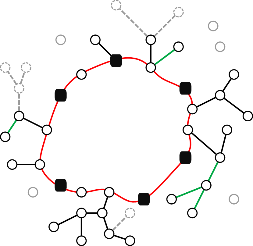
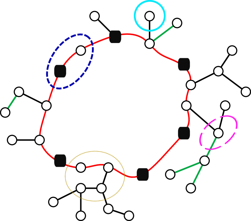
While it is convenient to think of as a cycle, note that the paths are not necessarily vertex disjoint. However, we can guarantee that is a Eulerian multigraph spanning all terminals. In the same sense, can be thought of as a collection of small trees which are all rooted at the cycle (in reality, some of those trees may intersect each other). In the following, we will call the edges of cycle edges and the edges of tree edges. A depiction of and can be seen in Fig. 1.
When we prune the trees into , the paths are not affected (because the pruning step guarantees that and stay connected in ). So our pruning step can only remove edges from . We thus define as the graph that is obtained by pruning all trees in with pruning threshold and then removing the cycle . We now partition the edge set of into layers. Intuitively, the -th layer of contains those edges that are contained in if and only if does not exceed some value .
Let be the -values of all vertices that might be affected by our pruning step, i.e., . By definition, we always have . Now let and for . One can see that is a partitioning of .
To be able to bound the cost of the cheapest -join , we define the following vector
| (1) |
where . To simplify future arguments, we also define the two components and of , as specified in (1). We remark that the vector has been used (for a different value of ) in [BKN24]. In Section 3.3, the cost of will be used as an upper bound for . To this end, we now prove the following lemma.
Lemma 5.
lies in the dominant of the -join polytope.
Proof.
First, observe that all coefficients are non-negative. We now consider an arbitrary for which is odd and show that .
We begin with the case where cuts the terminal set, i.e., where . In this case, separates at least two terminal pairs and , which implies and therefore . In the following we can thus assume that .
Now suppose that contains a pickup edge s.t. and . Recall that only spans vertices with . We therefore have which (by the connectivity constraints of (OLP)) implies and therefore .
It remains to show the bound for the case when only contains cycle and tree edges. By a simple counting argument, one can see that has the same parity as and therefore must be odd. Now observe that by our assumption, and that because is a Eulerian multigraph, must be even. If follows that must have an odd number of tree edges. We finish our proof by marginally adapting an argument from [BKN24]:
First, we consider the case where contains exactly one tree edge . This is only possible, if includes a whole subtree of one of the trees in . Because this subtree has survived the pruning step, must lie in some layer for which . Furthermore, if , then must contain at least one vertex with , which implies that . So we have
If, however, contains at least three tree edges, we know that all vertices have and that each tree edge contributes at least to . Therefore . ∎
(a)
(b)
3.3 Bounding the Tour Cost
In this section, we show the following bound on the cost of our computed tour:
Lemma 6.
The total cost of our computed tour can be bounded from above by
Our bound on the cost of is given by the cost of the parity correction vector . We start by analyzing the expected combined value of and .
Lemma 7.
where denotes the approximation guarantee of the current best PCTSP algorithm.
The main idea of the proof of Lemma 7 is that the weight which each layer is assigned in is large when is small and vice versa. At the same time, the chance for layer to be present after pruning and thus to contribute at all to both and is an increasing function of . By balancing out these two values, we obtain an upper bound or the contribution of all layers in to . At the same time we take into account that the cycle only contributes toward but crucially not towards the cost of the parity correction vector. This is where we utilize our assumption that and therefore also can be lower bounded by a constant fraction of opt. For formally proving Lemma 7, we need the following technical Lemma 8.
Lemma 8.
For , the function attains its maximum value over the interval at
Proof.
First, observe that and therefore
The claim follows from proving that is monotonously increasing on by showing that its derivative is strictly positive:
| (2) | ||||
| (3) |
where denotes the density function of . In (2) we used that for
Furthermore, (3) follows because and are determined by :
We obtain the function
The derivative of this function
is smaller than zero for , i.e., the function is monotonously decreasing. Therefore there is only one root in this range and one can easily check that it is located at . ∎
Proof of Lemma 7.
Our analysis follows the basic approach from [BKN24], but distinguishes between the cycle and the remaining part of the sampled solution to leverage the lower bound on the the cost of the cycle, which we get by running the simple algorithm from Section 2 in parallel. Another difference to [BKN24] is that is not a single tree, but consists of distinct sampled trees, which requires some additional notation.
Let denote the set of all possible outcomes obtained by sampling the trees as described in Section 2. One can see that the probability of a fixed outcome is and that .
Recall that technically, the subgraphs as well as the layers depend on the combination of sampled trees . We therefore write, e.g., to refer to the concrete cycle that arises from sampling the trees in . Now
| (4) | ||||
In (4) we used the fact from Lemma 8 that is maximized at and that the layers partition the edge set of . Now recall that we may assume that , which yields a bound of
∎
We will next analyze the cost of , in Lemma 9. The proof builds on the following theorem.
Theorem 3 (Böhm et al. [BFMS25]).
Let . Furthermore, let be a randomly chosen subset such that for each . Let and denote the the cheapest -rooted spanning forest and the cheapest -rooted spanning forest of respectively. Then .
Lemma 9.
For a fixed value of , the cost of is at most .
Proof.
We invoke Theorem 3 with , and . Recall that our pickup forest is the cheapest rooted spanning forest of and observe that . By Lemma 4, each vertex is not in sampled (and therefore not in ) with probability at most . It remains to show that the cost of the cheapest -rooted spanning forest of is at most .
As we have observed already in Section 2, the cost of the cheapest -rooted spanning forest of is equal to the cost of a minimum spanning tree in the graph obtained by contracting all vertices of into a single vertex , i.e., on . Furthermore, we have also observed that by applying the very same contraction to our solution (), we obtain a feasible solution to the (non-ordered) PCTSP relaxation. By splitting off all vertices in and scaling up by a factor of , we obtain a vector for which for all , i.e., a feasible point in the dominant555It is possible to obtain a feasible point in the polytope itself by applying a sequence of splitting-off operations. of the subtours elimination polytope of .
The cost of the minimum spanning tree on is therefore at most , which concludes the proof. ∎
Equipped with this upper bound, we can now bound the expected cost of , utilizing the density function and integrating over the range from which is drawn:
| (5) |
For the last equality we have used the definition of . We emphasize that by randomizing the choice of instead of flatly using , we have gained a factor of . In a similar way, we can use Lemma 9 to compute the expected cost of .
Lemma 10.
Proof.
Note that when , then is by definition the zero-vector. We compute
∎
Finally, we are able to combine the bounds on the various parts of , and obtain our final upper bound on the expected tour cost:
Note that the values of and are functions of . We therefore can express our upper bound as . By Lemma 3, Algorithm 1 pays at most times the penalty incurred by . Running Algorithm 1 with and determined by the single parameter thus yields an approximation factor of . Recall that the value of is currently slightly below . For , the term is minimized at . In fact, if we set , the term evaluates to .
For and , we have and . Thus we have proven Theorem 1.
4 Prize-collecting Multi-Path TSP
PC-Multi-Path-TSP can be modeled as the following linear program (kLP). {mini*} ∑e ∈E ∑i = 1k ce xi, e + ∑v ∈V-T πv (1 - yv) \addConstrainty_v= ∑_i = 1^k y_i, v ∀v ∈V \addConstraint(x_i, y_i) lies in the s_i-t_i-stroll relaxation
Similar to [BFMS25], we describe two algorithms for the problem and show that an appropriate combination of the two algorithms gives an -approximation.
In one algorithm, (which we call Algorithm ), we first sample trees using Lemma 2 and an optimal solution of (kLP), where tree connects terminals . The remaining vertices are picked up in a probabilistic fashion akin to Algorithm 1, i.e., we choose a random threshold and buy a -rooted spanning forest of . Here, is a constant whose value will be determined later. Then we double every edge that does not, for any , lie on the - path in . This gives a tour . Define and . Then it is easy to see that
One can already see that intuitively, this yields good results whenever is large.
Now we define the distribution from which is drawn. We choose s.t. where
Note that except for the constant , this is exactly the same distribution that we used in Algorithm 1. In fact, if we define , we obtain (compare this to ) so any result about obtained in the previous setting carries over to if we replace by . We remark that we use instead of because unlike in the previous case, will not be our final approximation factor.
We can thus bound the expected cost of in the same way as we did for PCOTSP. This is possible because the distribution as well as the (lower bound on the) probability of a vertex sampled at least once are the same as in Section 3.3.
First, we prove an equivalent of Lemma 9 i.e. we show that for any fixed value of , and then we compute the expected cost by integrating over the range from which is chosen as we have done in Eq. 5. This gives us the following upper bound on the expected tour cost:
Furthermore, by similar reasoning as in Section 3.1, we know that the expected total penalty paid by this algorithm is at most times the fractional penalty cost incurred by .
Now we give a simple Algorithm that works well when is small. Contract all the terminals into one mega-vertex with penalty , solve the PCTSP LP for this instance, and sample a tree from the solution. Double every edge in (obtained in the original graph), and then add the edges to get a final solution . It is easy to see that and that the incurred penalty is no higher than the fractional penalty cost of .
Running both algorithms and and returning each solution with probability , yields a tour of expected cost and an expected total penalty cost of at most
The approximation ratio that we get from combining both algorithms is
which is minimized at . This yields an approximation guarantee slightly below , proving Theorem 2.
5 Discussion
The PCOTSP, as a generalization of both PCTSP and OTSP, poses the challenges of each of the individual problems plus new challenges. The best approximation algorithms for OTSP ([BFMS25, AMN24]) both pick up vertices which have been left out of sampling, which imposes a cost of over the solution. In the latest PCTSP result ([BN23]), the cost of parity correction is slightly below . Hence, even without considering the specific characteristics of PCOTSP, utilizing the techniques of the latest results for the two problems brings the approximation factor close to 2. But note that in PCOTSP, the picking up of vertices is more complicated because the vertices are not necessarily wholly covered fractionally, and the need for parity correction for picked up vertices adds further complications which are absent from PCTSP.
It is not difficult to see that for the special cases of PCTSP, OTSP, our algorithms produce the best previously-known approximation factors for these problems. For example, when , PCOTSP is simply PCTSP. In this case, the cycle length over the one vertex is zero, and the output of our algorithm would be no worse than the output PCTSP algorithm of [BKN24] on the remaining vertices. Likewise, setting all penalties to turns PCOTSP into OTSP (and thus all values are 1). Thus all vertices that have not been sampled will be picked up (i.e., ), and no vertex is split off. This is equivalent to the algorithms of [BFMS25] and [AMN24]. In a similar vein, setting all penalties to turns PC-Multi-Path-TSP into Multi-Path-TSP, and here our algorithm would do the same as the factor algorithm of [BFMS25]. Their factor algorithm, however, does not directly carry over to our setting. The issue is that in the prize collecting setting, we require a picking-up step which leads to additional costs exceeding the additional gains as soon as we have to sample more than one tree.
It is an intriguing open question whether the problem admits an approximation factor of 2 or below, which we believe requires improvements of at least one of PCTSP or OTSP. Likewise, finding a good lower bound on the integrality gap of current LP relaxation would be very interesting.
References
- [ABHK11] Aaron Archer, MohammadHossein Bateni, MohammadTaghi Hajiaghayi, and Howard Karloff. Improved approximation algorithms for prize-collecting Steiner tree and TSP. SIAM journal on computing, 40(2):309–332, 2011.
- [AGH+24a] Ali Ahmadi, Iman Gholami, MohammadTaghi Hajiaghayi, Peyman Jabbarzade, and Mohammad Mahdavi. 2-approximation for prize-collecting steiner forest. In Proceedings of the 2024 Annual ACM-SIAM Symposium on Discrete Algorithms (SODA), pages 669–693. SIAM, 2024.
- [AGH+24b] Ali Ahmadi, Iman Gholami, MohammadTaghi Hajiaghayi, Peyman Jabbarzade, and Mohammad Mahdavi. Prize-collecting steiner tree: A 1.79 approximation. In Proceedings of the 56th Annual ACM Symposium on Theory of Computing, pages 1641–1652, 2024.
- [AMN24] Susanne Armbruster, Matthias Mnich, and Martin Nägele. A (3/2+ 1/e)-approximation algorithm for ordered TSP. In Approximation, Randomization, and Combinatorial Optimization. Algorithms and Techniques (APPROX/RANDOM 2024). Schloss Dagstuhl–Leibniz-Zentrum für Informatik, 2024.
- [BFMS25] Martin Böhm, Zachary Friggstad, Tobias Mömke, and Joachim Spoerhase. Approximating traveling salesman problems using a bridge lemma. In Proceedings of the 2025 Annual ACM-SIAM Symposium on Discrete Algorithms (SODA). SIAM, 2025. To appear.
- [BGSLW93] Daniel Bienstock, Michel X Goemans, David Simchi-Levi, and David Williamson. A note on the prize collecting traveling salesman problem. Mathematical programming, 59(1):413–420, 1993.
- [BHKK06] Hans-Joachim Böckenhauer, Juraj Hromkovič, Joachim Kneis, and Joachim Kupke. On the approximation hardness of some generalizations of TSP. In Algorithm Theory–SWAT 2006: 10th Scandinavian Workshop on Algorithm Theory, Riga, Latvia, July 6-8, 2006. Proceedings 10, pages 184–195. Springer, 2006.
- [BJFJ95] Jørgen Bang-Jensen, András Frank, and Bill Jackson. Preserving and increasing local edge-connectivity in mixed graphs. SIAM Journal on Discrete Mathematics, 8(2):155–178, 1995.
- [BKN24] Jannis Blauth, Nathan Klein, and Martin Nägele. A better-than-1.6-approximation for prize-collecting TSP. In International Conference on Integer Programming and Combinatorial Optimization, pages 28–42. Springer, 2024.
- [BMS13] Hans-Joachim Böckenhauer, Tobias Mömke, and Monika Steinová. Improved approximations for TSP with simple precedence constraints. J. Discrete Algorithms, 21:32–40, 2013.
- [BN23] Jannis Blauth and Martin Nägele. An improved approximation guarantee for prize-collecting TSP. In Proceedings of the 55th Annual ACM Symposium on Theory of Computing, pages 1848–1861, 2023.
- [Chr22] Nicos Christofides. Worst-case analysis of a new heuristic for the travelling salesman problem. Operations Research Forum, 3(1):20, 2022.
- [Goe09] Michel X Goemans. Combining approximation algorithms for the prize-collecting TSP. arXiv preprint arXiv:0910.0553, 2009.
- [GW95] Michel X Goemans and David P Williamson. A general approximation technique for constrained forest problems. SIAM Journal on Computing, 24(2):296–317, 1995.
- [KKO21] Anna R Karlin, Nathan Klein, and Shayan Oveis Gharan. A (slightly) improved approximation algorithm for metric TSP. In Proceedings of the 53rd Annual ACM SIGACT Symposium on Theory of Computing, pages 32–45, 2021.
- [PS15] Ian Post and Chaitanya Swamy. Linear programming-based approximation algorithms for multi-vehicle minimum latency problems (extended abstract). In Piotr Indyk, editor, Proceedings of the Twenty-Sixth Annual ACM-SIAM Symposium on Discrete Algorithms, SODA 2015, San Diego, CA, USA, January 4-6, 2015, pages 512–531. SIAM, 2015.
- [Ser78] AI Serdjukov. Some extremal bypasses in graphs [in russian]. Upravlyaemye Sistemy, 17(89):76–79, 1978.
- [TV24] Vera Traub and Jens Vygen. Approximation Algorithms for Traveling Salesman Problems. Cambridge University Press, 2024.
- [TVZ20] Vera Traub, Jens Vygen, and Rico Zenklusen. Reducing path TSP to TSP. In Proceedings of the 52nd Annual ACM SIGACT Symposium on Theory of Computing, pages 14–27, 2020.