aainstitutetext: Institut für Theoretische Physik, Universität Regensburg, D-93040 Regensburg, Germanybbinstitutetext: Institute of Particle and Nuclear Physics, Henan Normal University, Xinxiang 453007, Henan, P. R. Chinaccinstitutetext: II. Institut für Theoretische Physik, Universität Hamburg, D-22761 Hamburg, Germany

DESY 24-178
The two-loop coefficient functions for double deeply virtual Compton scattering

Vladimir M. Braun b    Hua-Yu Jiang c    Alexander N. Manashov a    and Andreas von Manteuffel vladimir.braun@ur.de jianghuayu@htu.edu.cn alexander.manashov@desy.de manteuffel@ur.de
Abstract

Making use of conformal symmetry of large-$n_{f}$ QCD in $d=4-2\epsilon$ dimensions at the Wilson-Fischer fixed point, we calculate the two-loop coefficient functions in the operator product expansion of two electromagnetic currents in general kinematics with two different photon virtualities. This result is necessary for the description of the double deeply virtual Compton scattering to the next-to-next-to-leading order accuracy, but is also interesting for a range of other two-photon processes. We present analytic expression for the coefficient function in momentum fraction space in the $\overline{\text{MS}}$ scheme and study its numerical impact on the Compton form factors for a simple model of the generalized parton distributions. The calculated corrections turn out to be large and are significant for the kinematics of proposed experiments.

Keywords:
DVCS, conformal symmetry, generalized parton distributions

1 Introduction

Deeply-virtual Compton scattering (DVCS) Ji:1996nm ; Radyushkin:1996nd ; Mueller:1998fv is generally accepted to be the “gold-plated” process with the highest potential impact on the determination of the generalized parton distributions (GPDs) in the nucleon. The problem is, however, that at leading order (LO) the DVCS and time-like Compton scattering (TCS) amplitudes only involve GPDs at the $x=\xi$ line, where $x$ is the average parton momentum and $\xi$ is the asymmetry parameter. The double deeply virtual Compton scattering $\gamma^{\ast}(q_{1})+N(p_{1})\to\gamma^{\ast}(q_{2})+N(p_{2})$ (DDVCS) avoids this restriction Belitsky:2002tf ; Guidal:2002kt and can be accessed by studying exclusive electroproduction of a lepton pair. Varying the invariant mass of the lepton pair, one can, in principle, directly extract the GPDs from the observables. DDVCS can be measured in near future at both fixed target Zhao:2021zsm and collider facilities AbdulKhalek:2021gbh ; Anderle:2021wcy . A preliminary impact study of DDVCS phenomenology for the JLAB12, JLAB20+ and EIC kinematics Deja:2023ahc reached promising conclusions.

The main challenge of all GPD studies is that the quantities of interest are functions of three kinematic variables. Their extraction requires a massive amount of data and very high precision for both experimental and theory inputs. The future GPD determinations will therefore have to be based on global fits of all available experiments and the constraints from lattice measurements and PDFs in the forward limit. It is imperative that all ingredients in such fits are calculated with the same precision. Ideally, one would like to reach the same level of accuracy as in inclusive reactions, where the next-to-next-to leading order (NNLO) analysis has become the standard in the field Accardi:2016ndt . One-loop DVCS coefficient functions have been known for a long time Ji:1997nk ; Belitsky:1997rh and the two-loop ones have been calculated recently Braun:2020yib ; Gao:2021iqq ; Braun:2021grd ; Braun:2022bpn ; Ji:2023xzk . Two-loop evolution equations for the GPDs are known from Belitsky:1998gc ; Belitsky:1999hf . Three-loop evolution equations for flavor-nonsinglet GPDs in position space have been derived in Braun:2017cih ; Ji:2023eni and for the first few moments of flavor-singlet GPDs in Braun:2022byg . The DDVCS description has to be extended to the same level of accuracy. As the first step in this direction, in this work we calculate the two-loop DDVCS coefficient functions (CFs) for the flavor-nonsinglet vector contributions using conformal symmetry techniques.

The idea to apply the conformal symmetry to off-forward reactions is not new but the early work Brodsky:1984xk was missing an important element: the scheme-dependent difference between the dilatation and special conformal anomalies Mueller:1991gd . It was first shown in Belitsky:1997rh that conformal symmetry provides a connection between the CFs in DVCS and DIS. The general strategy of our calculation follows Ref. Braun:2020yib , but involves some new technical elements. We make use of conformal symmetry of large-$n_{f}$ QCD in non-integer $d=4-2\epsilon$ dimensions at the Wilson-Fischer fixed point Braun:2013tva ; Braun:2018mxm . In a conformal theory the contributions of operators with total derivatives are related to the contributions of the operators without total derivatives by symmetry transformations and do not need to be calculated separately. In this way, the calculation of the $\ell$-loop off-forward CF can be reduced to the $\ell$-loop forward CF, known from DIS, and the $(\ell-1)$-loop calculation of the off-forward CF in $4-2\epsilon$ dimensions, including terms $\mathcal{O}(\epsilon^{\ell-1})$.

The presentation is organized as follows. Section 2 is introductory, it contains general definitions and specifies our notation and conventions. In Sect. 3 we present the general framework and the procedure for the calculation of CFs in the OPE of two electromagnetic currents using conformal symmetry of QCD at the Wilson-Fischer fixed point in non-integer dimensions. A new ansatz for the solution is presented, which allows one to solve the relevant equations for the case of arbitrary photon virtualities. Section 4 is devoted to the particularities of the two-loop calculation and the discussion of the mathematical structure of the results. Explicit expressions for the CFs in momentum fraction space are presented in Appendix E and in two ancillary files using different representations for the relevant generalized polylogarithms. Numerical estimates of the size of the two-loop correction for realistic kinematics are presented in Sect. 5. The final Sect. 6 is reserved for a short summary. The paper also contains several Appendices explaining the construction of helicity amplitudes, some useful integrals, expansion of the CFs in the threshold region, and more.

2 Kinematics, notation and conventions, and one-loop results

The generalized Compton amplitude is given by a Fourier transform of the off-forward matrix element of the time-ordered product of two electromagnetic currents,

$\displaystyle A_{\mu\nu}$ $\displaystyle=i\int d^{4}x\,e^{iq_{1}\cdot x}\big{\langle}p_{2}\big{\lvert}T\big{\{}j_{\mu}^{\mathrm{em}}(x)\,j_{\nu}^{\mathrm{em}}(0)\big{\}}\big{\rvert}p_{1}\big{\rangle},$ (1)

corresponding to the double deeply virtual Compton scattering process

$$\gamma^{\ast}(q_{1})+N(p_{1})\rightarrow\gamma^{\ast}(q_{2})+N(p_{2})\,.$$ (2)

Here $q_{1}$ and $q_{2}$ are the momenta of the incoming and outgoing photons, respectively, $p_{1},p_{2}$ are the target (nucleon) momenta in initial and final states, and $q_{2}=p_{1}+p_{2}-q_{1}$. Let

$\displaystyle q=\frac{1}{2}(q_{1}+q_{2}),\qquad p=\frac{1}{2}(p_{1}+p_{2}),\qquad\Delta=p_{2}-p_{1}=q_{1}-q_{2}\,,\qquad Q^{2}=-q^{2},$ (3)

and

$\displaystyle\xi=-\frac{\Delta\cdot q}{2p\cdot q},\qquad\eta=\frac{Q^{2}}{2p\cdot q},\qquad\omega=\frac{\xi}{\eta}=\frac{q_{1}^{2}-q_{2}^{2}}{q_{1}^{2}+q_{2}^{2}-\Delta^{2}/2}.$ (4)

In the following we assume $\Delta^{2}=0$.

The DVCS corresponds to $\omega=1$ such that $\eta=\xi\simeq x_{B}/(2-x_{B})$, DIS corresponds to $\xi=0$, $\eta=x_{B}$, TCS corresponds to $\omega=-1$, and exclusive electroproduction of a lepton pair (DDVCS) to $\omega<-1$. For all processes of interest $q_{1}^{2}-q_{2}^{2}<0$ and $0<\xi<1$.

In the leading-twist approximation, the parity-even (vector) part of the DDVCS amplitude can be written in terms of two Compton form factors (CFFs), e.g. Belitsky:2005qn

$\displaystyle A^{\mu\nu}$ $\displaystyle=\left(-g^{\mu\nu}+\frac{q_{2}^{\mu}q_{1}^{\nu}}{(q_{1}\cdot q_{2})}\right)\mathcal{F}_{1}(\xi,\eta,\Delta^{2},Q^{2})+\frac{2}{pq}\left(p^{\mu}+\frac{1}{2\eta}q_{2}^{\mu}\right)\left(p^{\nu}+\frac{1}{2\eta}q_{1}^{\nu}\right)\mathcal{F}_{2}(\xi,\eta,\Delta^{2},Q^{2}).$ (5)

A more convenient decomposition is in terms of the “transverse” and “longitudinal” CFFs defined as

$$\mathcal{F}_{\perp}=\mathcal{F}_{1}\,,\qquad\quad\mathcal{F}_{L}=\frac{1}{\eta}\mathcal{F}_{2}-\mathcal{F}_{1}\,.$$ (6)

For completeness, in Appendix A, we also discuss the decomposition of the amplitude $A^{\mu\nu}$ in terms of helicity amplitudes.

The factorization theorem Radyushkin:1997ki ; Ji:1998xh ; Collins:1998be relates flavor-nonsinglet contributions to the CFFs $\mathcal{F}_{i}$, $i=\perp,L$, to charge conjugation $C=+1$ combinations of quark GPDs

$\displaystyle\mathcal{F}_{i}(\xi,\eta,\Delta^{2},Q^{2})$ $\displaystyle=\sum_{q}e_{q}^{2}\int_{-1}^{1}\!\frac{dx}{\xi}\,C_{i}\left(\frac{x}{\eta},\frac{\xi}{\eta},\frac{Q^{2}}{\mu^{2}}\right)F_{q}^{(+)}(x,\xi,\Delta^{2},\mu^{2})\,,$
$\displaystyle F_{q}^{(+)}(x,\xi,\Delta^{2},\mu^{2})$ $\displaystyle=F_{q}(x,\xi,\Delta^{2},\mu^{2})-F_{q}(-x,\xi,\Delta^{2},\mu^{2})\,.$ (7)

The GPDs are defined by an appropriate matrix element of the light-ray operator

$\displaystyle\mathcal{O}_{q}(z_{1},z_{2})=\bar{q}(z_{1}n)\not{n}[z_{1}n,z_{2}n]q(z_{2}n)\,,$ (8)

where $n^{\mu}$ is a light-like vector, $[z_{1}n,z_{2}n]$ is the Wilson line. For our present purposes one can choose (see Appendix A) $n^{\mu}=q_{1}^{\mu}/q_{1}^{2}-q_{2}^{\mu}/q_{2}^{2}$ so that $\xi=-\Delta_{+}/(2p_{+})$ where $\Delta_{+}=\Delta\cdot n$ and $p_{+}=p\cdot n$. An off-forward matrix element of the renormalized light-ray operator (8) can be parametrized as follows:

$\displaystyle\langle p_{2}|[\mathcal{O}_{q}(z_{1},z_{2})]|p_{1}\rangle$ $\displaystyle=2p_{+}\int_{-1}^{1}dx\,e^{-ip_{+}\xi(z_{1}+z_{2})+ip_{+}x(z_{1}-z_{2})}\,F_{q}(x,\xi,\Delta^{2},\mu^{2})\,,$
$\displaystyle F_{q}^{(+)}(x,\xi,\Delta^{2},\mu^{2})$ $\displaystyle=F_{q}(x,\xi,\Delta^{2},\mu^{2})-F_{q}(-x,\xi,\Delta^{2},\mu^{2})\,.$ (9)

where the bracket $[\ldots]$ in the matrix element above stands for renormalization in the $\overline{\mathrm{MS}}$ scheme. The quark GPD for a nucleon can further be decomposed in contributions of the two Dirac structures $H_{q}(x,\xi)$ and $E_{q}(x,\xi)$Diehl:2003ny , but this decomposition is irrelevant for our present purposes.

The scale dependence of the GPDs is governed by the renormalization group equation (RGE)

$\displaystyle\left(\mu\frac{\partial}{\partial\mu}+\beta(\alpha_{s})\frac{\partial}{\partial\alpha_{s}}+\mathbb{H}\right)[\mathcal{O}_{q}(z_{1},z_{2})]=0\,,$ (10)

where $\mathbb{H}$ (evolution kernel) is an integral operator acting on the coordinates $z_{1},z_{2}$. Translation-invariant polynomials $z_{12}^{N}=(z_{1}-z_{2})^{N}$ are eigenfunctions of the evolution kernel and the corresponding eigenvalues define the anomalous dimensions of local operators with spin $N$,

$\displaystyle\mathbb{H}\,z_{12}^{N-1}=\gamma_{N}z_{12}^{N-1},$ (11)

see Braun:2017cih ; Braun:2020yib for the systematic presentation and details.

In what follows we drop electromagnetic charges and the sum over flavors, and introduce a notation

$\displaystyle z=x/\eta\,,\qquad\quad C_{i}\left(\frac{x}{\eta},\frac{\xi}{\eta},\frac{Q^{2}}{\mu^{2}}\right)\equiv C_{i}\left(z,\omega,\frac{Q^{2}}{\mu^{2}}\right)\,.$ (12)

The CFs do not depend on the target and can be calculated in perturbation theory

$\displaystyle C_{i}(z,\omega,Q^{2}/\mu^{2})=C^{(0)}_{i}(z)+a_{s}C^{(1)}_{i}(z,\omega,Q^{2}/\mu^{2})+a_{s}^{2}C^{(2)}_{i}(z,\omega,Q^{2}/\mu^{2})+\ldots,$ (13)

where

$\displaystyle a_{s}=\alpha_{s}(\mu)/(4\pi)\,.$ (14)

They are real functions in the Euclidean region $\omega\in[-1,1]$, $z\in(-1,1)$ and $Q^{2}>0$, and can be continued analytically Mueller:2012sma to the physical regions of different processes. Assuming $x$, $\xi>0$ and $q_{1}^{2}-q_{2}^{2}<0$ are real numbers and the usual causal prescription for $q_{1}^{2}+q_{2}^{2}\mapsto q_{1}^{2}+q_{2}^{2}+i0$ one obtains

$\displaystyle C_{i}\left(\frac{x}{\eta},\frac{\xi}{\eta},\frac{Q^{2}}{\mu^{2}}\right)$ $\displaystyle\mapsto C_{i}\left(\frac{x}{\eta-i0},\frac{\xi}{\eta-i0},\frac{Q^{2}}{\mu^{2}}-i0\right)=C_{i}\left(\frac{x}{\xi}(\omega+i0),\omega+i0,\frac{Q^{2}}{\mu^{2}}-i0\right).$ (15)

We have checked that the resulting one-loop CFs agree with the explicit evaluation in Minkowski space in Ref. Pire:2011st .

The tree-level CFs are well-known since the pioneering works Ji:1996nm ; Radyushkin:1996nd

$\displaystyle C_{\perp}^{(0)}(z,\omega)$ $\displaystyle=\frac{\omega}{1-z}-\frac{\omega}{1+z}\,,\qquad C_{L}^{(0)}(z,\omega)=0\,.$ (16)

We find it convenient to present the results for loop corrections in the following generic form to emphasize the symmetries and the structure of singularities:

$\displaystyle C_{i}^{(k)}\left(z,\omega,\frac{Q^{2}}{\mu^{2}}\right)$ $\displaystyle=\frac{C_{F}\,\omega}{1-z}\Big{[}A_{i}^{(k)}\left(z,\omega,\frac{Q^{2}}{\mu^{2}}\right)+A_{i}^{(k)}\left(z,-\omega,\frac{Q^{2}}{\mu^{2}}\right)\Big{]}$
$\displaystyle\quad+\frac{C_{F}}{\omega-z}\Big{[}B_{i}^{(k)}\left(z,\omega,\frac{Q^{2}}{\mu^{2}}\right)-B_{i}^{(k)}\left(-z,-\omega,\frac{Q^{2}}{\mu^{2}}\right)\Big{]}-(z\leftrightarrow-z)\,.$ (17)

The one-loop results have been available for a long time Ji:1997nk ; Mankiewicz:1997bk ; Belitsky:2005qn ; Pire:2011st :

$\displaystyle A_{\perp}^{(1)}\left(z,\omega,\frac{Q^{2}}{\mu^{2}}\right)$ $\displaystyle=\ln^{2}(1\!-\!z)-\ln^{2}(1\!-\!\omega)-\frac{3}{2}\ln(1\!-\!z)+3\ln(1\!-\!\omega)-\frac{9}{2}$
$\displaystyle\quad+2\ln\frac{Q^{2}}{\mu^{2}}\Big{[}\ln(1\!-\!z)-\ln(1\!-\!\omega)+\frac{3}{4}\Big{]},$
$\displaystyle B_{\perp}^{(1)}\left(z,\omega,\frac{Q^{2}}{\mu^{2}}\right)$ $\displaystyle=-\frac{1+\omega}{2}\Big{[}\ln^{2}(1\!-\!z)-\ln^{2}(1\!-\!\omega)\Big{]}+3\omega\Big{[}\ln(1\!-\!z)-\ln(1\!-\!\omega)\Big{]}$
$\displaystyle\quad-\ln\frac{Q^{2}}{\mu^{2}}(1+\omega)\Big{[}\ln(1\!-\!z)-\ln(1\!-\!w)\Big{]},$
$\displaystyle A_{L}^{(1)}\left(z,\omega,\frac{Q^{2}}{\mu^{2}}\right)$ $\displaystyle=0\,,$
$\displaystyle B_{L}^{(1)}\left(z,\omega,\frac{Q^{2}}{\mu^{2}}\right)$ $\displaystyle=2\Big{[}\ln(1\!-\!z)-\ln(1\!-\!w)\Big{]}\,.$ (18)

It is important that, despite the factor $1/(\omega-z)$ present in Eq. (2), the one-loop CFs are analytic functions at $z=\omega$. They are also analytic functions in the limit $\lambda\to 0$, rescaling $Q^{2}\mapsto\lambda Q^{2}$, $\omega\mapsto\omega/\lambda$, $z\mapsto z/\lambda$. The latter property ensures that collinear factorization holds at the kinematic point $q_{1}^{2}+q_{2}^{2}=0$, as expected from the leading regions analysis Belitsky:2005qn . We will find that the two-loop CFs have the same analytic properties.

The two-loop CFs contain contributions of three different color structures. We choose them as follows:

$\displaystyle C_{i}^{(2)}\Big{(}z,\omega,\frac{Q^{2}}{\mu^{2}}\Big{)}$ $\displaystyle=C_{F}\biggl{[}\beta_{0}C_{i}^{(2,\beta)}\Big{(}z,\omega,\frac{Q^{2}}{\mu^{2}}\Big{)}+C_{F}C_{i}^{(2,P)}\Big{(}z,\omega,\frac{Q^{2}}{\mu^{2}}\Big{)}+\frac{1}{N_{c}}C_{i}^{(2,NP)}\Big{(}z,\omega,\frac{Q^{2}}{\mu^{2}}\Big{)}\biggr{]},$ (19)

and use the same color decomposition for the $A_{i}^{(2)}$ and $B_{i}^{(2)}$ functions defined in Eq. (2), apart from the overall $C_{F}$ factor. The two-loop results turn out to be rather lengthy so that we write them separating the renormalization group (RG) logarithms, with the notation

$\displaystyle A_{i}^{(2)}\Big{(}z,\omega,\frac{Q^{2}}{\mu^{2}}\Big{)}$ $\displaystyle=A_{i}^{(2)}\left(z,\omega\right)+\ln\Big{(}\frac{Q^{2}}{\mu^{2}}\Big{)}A_{i,\ln}^{(2)}\left(z,\omega\right)+\ln^{2}\Big{(}\frac{Q^{2}}{\mu^{2}}\Big{)}A_{i,\ln^{2}}^{(2)}\left(z,\omega\right)\,,$ (20)

and similarly for $B_{i}^{(2)}$.

3 General framework

One can consider, formally, the two-photon reactions in a generic $4-2\epsilon$-dimensional theory. All definitions in Sec. 2 can be taken over without modifications except for that the CFs acquire an $\epsilon$-dependence so that

$$C_{i}(z,\omega,Q^{2}/\mu^{2},a_{s})\mapsto C_{i}(z,\omega,Q^{2}/\mu^{2},a_{s},\epsilon)\,.$$

Hence their perturbative expansion involves $\epsilon$-dependent coefficients:

$\displaystyle C(a_{s},\epsilon)$ $\displaystyle=C^{(0)}+a_{s}\,C^{(1)}(\epsilon)+a_{s}^{2}\,C^{(2)}(\epsilon)+\mathcal{O}(a_{s}^{3})\,,$
$\displaystyle C^{(k)}(\epsilon)$ $\displaystyle=C^{(k)}+\epsilon\,C^{(k,1)}+\epsilon^{2}C^{(k,2)}+\mathcal{O}(\epsilon^{3})\,.$ (21)

Note that the tree-level CF $C^{(0)}$ does not depend on $\epsilon$.

We are interested in the CFs in four dimensions as a function of the coupling, but as an intermediate step will calculate $C_{\ast}=C(\alpha_{s}^{*},\epsilon)$ on the line in the $(\epsilon,\alpha_{s})$ plane where $\beta(\alpha_{s}^{\ast})=0$ so that $\alpha_{s}^{\ast}=\alpha_{s}^{\ast}(\epsilon)$ (Wilson-Fisher fixed point) or, equivalently,

$\displaystyle\epsilon_{\ast}$ $\displaystyle=\epsilon_{\ast}(a_{s})=-\big{(}\beta_{0}a_{s}+\beta_{1}a_{s}^{2}+\ldots\big{)}\equiv-\bar{\beta}(a_{s})\,,\qquad\beta_{0}=\frac{11}{3}N_{c}-\frac{2}{3}n_{f}\,,$ (22)

with $N_{c}$ and $n_{f}$ being the numbers of colors and light flavors, respectively. Trading the $\epsilon$-dependence for the $a_{s}^{\ast}$ dependence one can write the CFs on this line as an expansion in the coupling alone,

$\displaystyle C_{\ast}(a_{s})$ $\displaystyle=C(a_{s},\epsilon_{\ast})=C^{(0)}+a_{s}C_{\ast}^{(1)}+a_{s}^{2}C_{\ast}^{(2)}+\mathcal{O}(a_{s}^{3})\,,$ (23)

where, obviously,

$\displaystyle C_{\ast}^{(1)}$ $\displaystyle=C^{(1)}\,,\qquad C_{\ast}^{(2)}=C^{(2)}-\beta_{0}C^{(1,1)}\,,$ (24)

or, equivalently

$\displaystyle C^{(1)}$ $\displaystyle=C_{\ast}^{(1)}\,,\qquad C^{(2)}=C_{\ast}^{(2)}+\beta_{0}C^{(1,1)}\,.$ (25)

The rationale for organizing the calculation in this way is that QCD at the Wilson-Fischer critical point is conformally invariant Fortin:2012hn ; Braun:2018mxm . Conformal symmetry allows one to obtain the coefficients $C_{\ast}^{(2)}$ from the known results from DIS avoiding explicit calculation. To restore the result in 4 dimensions one also needs to know terms of order $\epsilon$ in the one-loop CFs. This additional calculation is, however, rather simple.

It is straightforward to continue this construction to higher orders. The general statement is that the $\ell$-loop off-forward CFs in QCD in $d=4$ in the $\overline{\text{MS}}$ scheme can be obtained from the corresponding result in conformal theory (alias from the corresponding CFs in the forward limit), adding terms proportional to the QCD beta-function. Such extra terms require the calculation of the corresponding $(\ell-1)$-loop off-forward CFs in $d=4-2\epsilon$ dimensions expanded to order $\epsilon^{\ell-1}$.

3.1 Conformal OPE

The OPE for the product of currents has a generic form, schematically

$\displaystyle T\{j^{\rm em}_{\mu}(x)j^{\rm em}_{\nu}(0)\}$ $\displaystyle=\sum_{N,k}C_{N,k}\partial_{+}^{k}\mathcal{O}_{N}(0)\,,$ (26)

where $\mathcal{O}_{N}(0)$ are local operators of increasing dimension and $C_{Nk}$ are the corresponding CFs. The power of conformal symmetry is that it allows one to restore the contributions of all operators containing total derivatives from the ones without total derivatives, i.e. restore $C_{N,k}$ from $C_{N,0}$ using conformal algebra Ferrara:1972uq .

Retaining the contributions of twist-two vector operators only, the result reads Braun:2020yib

$\displaystyle\text{T}\,\big{\{}j^{\mu}(x_{1})j^{\nu}(x_{2})\big{\}}$ $\displaystyle=\sum_{N,\text{even}}\frac{\mu^{\gamma_{N}}}{(-x_{12}^{2}+i0)^{t_{N}}}\int_{0}^{1}du\Biggl{\{}-\frac{1}{2}A_{N}(u)\left(g^{\mu\nu}-\frac{2x_{12}^{\mu}x_{12}^{\nu}}{x_{12}^{2}}\right)+B_{N}(u)g^{\mu\nu}$
$\displaystyle\quad+C_{N}(u)x_{12}^{\nu}\partial_{1}^{\mu}-C_{N}(1-u)x_{12}^{\mu}\partial_{2}^{\nu}+D_{N}(u)x_{12}^{2}\partial_{1}^{\mu}\partial_{2}^{\nu}\Biggr{\}}\mathcal{O}_{N}^{x_{12}\ldots x_{12}}(x_{21}^{u})\,,$ (27)

where

$\displaystyle\partial^{\mu}_{k}=\frac{\partial}{\partial x^{\mu}_{k}},\qquad\quad x_{12}=x_{1}-x_{2}\,,\qquad\quad x_{21}^{u}=(1-u)x_{2}+ux_{1}\,,$ (28)

and

$\displaystyle\mathcal{O}_{N}^{x\ldots x}(y)=x_{\mu_{1}}\ldots x_{\mu_{N}}\mathcal{O}_{N}^{\mu_{1}\ldots\mu_{N}}(y)\,.$ (29)

Further, $\mathcal{O}_{N}^{\mu_{1}\ldots\mu_{N}}(y)$ are the leading-twist conformal operators that transform in the proper way under conformal transformations

$\displaystyle[\mathbb{K}_{\mu},\mathcal{O}_{N}^{x\ldots x}(y)]=\left(2y_{\mu}y^{\nu}\frac{\partial}{\partial y^{\nu}}-y^{2}\frac{\partial}{\partial y^{\mu}}+2\Delta_{N}y_{\mu}+2y^{\nu}\left(x_{\mu}\frac{\partial}{\partial x^{\nu}}-x_{\nu}\frac{\partial}{\partial x^{\mu}}\right)\right)\mathcal{O}_{N}^{x\ldots x}(y).$ (30)

Here and below, $N$ is the spin and $\Delta_{N}$ the scaling dimension of $\mathcal{O}_{N}^{\mu_{1}\ldots\mu_{N}}$, $\Delta_{N}=d_{\ast}+N-2+\gamma_{N}$ where $d_{\ast}=4-2\epsilon_{\ast}$, $\gamma_{N}=\gamma_{N}(a_{s})$ is the anomalous dimension, $t_{N}=2-\epsilon_{\ast}-\frac{1}{2}\gamma_{N}(a_{s})$ is the twist and $j_{N}=N+1-\epsilon_{\ast}+\frac{1}{2}\gamma_{N}(a_{s})$ is the conformal spin. We have separated in Eq. (3.1) the scale factor $\mu^{\gamma_{N}}$ to make the invariant functions $A_{N}(u),\ldots,D_{N}(u)$ dimensionless. Note that only vector operators with even spin $N$ contribute to the expansion.

Conformal invariance and current conservation $\partial^{\mu}j_{\mu}=0$ constrain the functional form of the invariant functions $A_{N}(u),\ldots,D_{N}(u)$ in Eq. (3.1) and also lead to certain relations between them. One obtains Braun:2020yib

$\displaystyle A_{N}(u)=a_{N}(a_{s})\,u^{j_{N}-1}(1-u)^{j_{N}-1}\,,$ $\displaystyle B_{N}(u)=b_{N}(a_{s})u^{j_{N}-1}(1-u)^{j_{N}-1}\,.$ (31)

Explicit expressions for $C_{N}(u)$ and $D_{N}(u)$ can be found in Ref. (Braun:2020yib, , Eq. (3.12)) and do not involve new parameters. Thus the OPE of the product of two conserved spin-one currents in a generic conformal theory involves two constants, $a_{N}(a_{s})$ and $b_{N}(a_{s})$, for each (even) spin $N$. In QCD the expansion of $a_{N}(a_{s})$ starts at order $\mathcal{O}(a_{s})$.

For the matrix elements between states with the same momentum (forward scattering), the position of the operators on the r.h.s of Eq. (3.1) is irrelevant and the integration over the $u$-variable can be taken explicitly. It is convenient to fix the normalization of the operators such that

$\displaystyle\mathcal{O}_{N}^{\mu_{1}\ldots\mu_{N}}(0)=i^{N-1}\bar{q}(0)\gamma^{\{\mu_{1}}D^{\mu_{2}}\ldots D^{\mu_{N}\}}q(0)+\,\text{total~{}derivatives}\,,$ (32)

where $D^{\mu}=\partial^{\mu}+igA^{\mu}$ and $\{\ldots\}$ denotes the symmetrization of all enclosed Lorentz indices and the subtraction of traces. In this way the forward matrix elements of these operators can be identified with the moments of quark parton distributions (PDFs)

$\displaystyle\langle p|\mathcal{O}_{N}^{\mu_{1}\ldots\mu_{N}}(0)|p\rangle=p^{\{\mu_{1}}\ldots p^{\mu_{N}\}}f_{N}\,.$ (33)

With this normalization one obtains Braun:2020yib

$\displaystyle T_{\mu\nu}(p,q)$ $\displaystyle\equiv i\int d^{d}x\,e^{-iqx}\langle p|T(j_{\mu}(x)j_{\nu}(0)|p\rangle$
$\displaystyle=\sum_{N,\text{even}}\!\!\frac{f_{N}}{x_{B}^{N}}\left(\frac{\mu}{Q}\right)^{\gamma_{N}}\!\biggl{[}\left(-g_{\mu\nu}+\frac{q_{\mu}q_{\nu}}{q^{2}}\right)c_{1N}(a_{s})+\frac{(q_{\mu}\!+\!2x_{B}p_{\mu})(q_{\nu}\!+\!2x_{B}p_{\nu})}{Q^{2}}c_{2N}(a_{s})\biggr{]},$ (34)

where $x_{B}=Q^{2}/(2qp)$ is the Bjorken scaling variable and

$\displaystyle c_{1N}$ $\displaystyle=i^{N}\pi^{d/2}2^{\gamma_{N}}B(j_{N},j_{N})\frac{\Gamma(N+\gamma_{N}/2)}{\Gamma(t_{N})}\left(\frac{t_{N}-1}{2t_{N}}a_{N}-b_{N}\right),$
$\displaystyle c_{2N}$ $\displaystyle=i^{N}\pi^{d/2}2^{\gamma_{N}}B(j_{N},j_{N})\frac{\Gamma(N+\gamma_{N}/2)}{\Gamma(t_{N})}\left(-b_{N}+\frac{2N+d-t_{N}-1}{2t_{N}}a_{N}\right).$ (35)

Here and below $B(j_{N},j_{N})$ is the Euler Beta function.

Comparing this expression with the usual expansion for the DIS structure functions, see e.g. Vermaseren:2005qc , we can identify

$\displaystyle c_{2N}(a_{s})\left(\frac{\mu}{Q}\right)^{\gamma_{N}}$ $\displaystyle=C_{2}^{\mathrm{\scriptscriptstyle DIS}}\left(N,\frac{Q^{2}}{\mu^{2}},a_{s},\epsilon_{\ast}\right),$
$\displaystyle c_{1N}(a_{s})\left(\frac{\mu}{Q}\right)^{\gamma_{N}}$ $\displaystyle=C_{2}^{\mathrm{\scriptscriptstyle DIS}}\left(N,\frac{Q^{2}}{\mu^{2}},a_{s},\epsilon_{\ast}\right)-C_{L}^{\mathrm{\scriptscriptstyle DIS}}\left(N,\frac{Q^{2}}{\mu^{2}},a_{s},\epsilon_{\ast}\right)\equiv C_{1}^{\mathrm{\scriptscriptstyle DIS}}\left(N,\frac{Q^{2}}{\mu^{2}},a_{s},\epsilon_{\ast}\right).$ (36)

where $C_{2}^{\mathrm{\scriptscriptstyle DIS}}$ and $C_{L}^{\mathrm{\scriptscriptstyle DIS}}$ are the familiar CFs for the structure functions $F_{2}$ and $F_{L}$, respectively, (in $4-2\epsilon_{\ast}$ dimensions) that are known to third order in the QCD coupling. With this identification, the structure of the OPE for the product of two vector currents in conformal QCD is completely fixed.

For the off-forward case there are two modifications. First, the position of the operator $\mathcal{O}_{N}(ux)$ in Eq. (3.1) becomes relevant since

$\displaystyle\langle p_{2}|\mathcal{O}_{N}(x_{21}^{u})|p_{1}\rangle=e^{i(x_{21}^{u}\cdot\Delta)}\langle p_{2}|\mathcal{O}_{N}(0)|p_{1}\rangle\,,$ (37)

producing a $u$-dependent shift of the momentum in the Fourier integral. Second, the matrix element becomes more complicated. It can be parameterized as

$\displaystyle\langle p_{2}|n^{\mu_{1}}\ldots n^{\mu_{N}}\mathcal{O}_{\mu_{1}\ldots\mu_{N}}(0)|p_{1}\rangle$ $\displaystyle=\sum_{k}\left(-\frac{1}{2}\right)^{k}f_{N}^{(k)}p_{+}^{N-k}\Delta_{+}^{k}=p_{+}^{N}f_{N}(\xi)\,,$
$\displaystyle f_{N}(\xi)$ $\displaystyle\equiv\sum_{k}f_{N}^{(k)}\xi^{k}\,,\qquad f_{N}^{(0)}=f_{N}^{\rm DIS}\,.$ (38)

The leading-twist CFFs $\mathcal{F}_{1}(\xi,\eta,\Delta^{2},Q^{2})$ and $\mathcal{F}_{L}(\xi,\eta,\Delta^{2},Q^{2})$ (5) can be separated by taking $g_{\perp}^{\mu\nu}\mathcal{A}_{\mu\nu}$ and $\Delta^{\mu}\mathcal{A}_{\mu\nu}\Delta^{\nu}$ projections, respectively. In this way the (complicated) $C_{N}(u)$ and $D_{N}(u)$ terms in (3.1) drop out, and one obtains after a short calculation

$\displaystyle\mathcal{F}^{\ast}_{\perp}(\xi,\eta,Q^{2})$ $\displaystyle=\sum_{N}f_{N}(\xi)\eta^{-N}\frac{C_{1}^{\mathrm{\scriptscriptstyle DIS}}(N,\tfrac{Q^{2}}{\mu^{2}},a_{s},\epsilon_{\ast})}{(1+w)^{\tfrac{1}{2}\gamma_{N}+N}}{}_{2}F_{1}\left(\tfrac{1}{2}\gamma_{N}+N,j_{N},2j_{N},\frac{2w}{1+w}\right),$ (39)
$\displaystyle\mathcal{F}^{\ast}_{L}(\xi,\eta,Q^{2})$ $\displaystyle=\sum_{N}f_{N}(\xi)\eta^{-N}\frac{C_{L}^{\mathrm{\scriptscriptstyle DIS}}(N,\tfrac{Q^{2}}{\mu^{2}},a_{s},\epsilon_{\ast})}{(1+w)^{\tfrac{1}{2}\gamma_{N}+N+1}}{}_{2}F_{1}\left(\tfrac{1}{2}\gamma_{N}+N+1,j_{N},2j_{N},\frac{2w}{1+w}\right),$ (40)

where the superscript indicates that these results refer to QCD at the critical point. Hereafter we do not show the dependence of the CFFs on $\Delta^{2}$, which only enters through the matrix elements and does not affect CFs.

3.2 Coefficient functions in momentum fraction space: master equation

As the next step, we have to find a way to obtain the CFs in momentum fraction space $C_{1,L}(z,w)$ starting from these expressions. To this end one needs to write the GPD in terms of the matrix elements of conformal operators, which is difficult. The form of these operators is determined by the generator of special conformal transformation, which is modified in an interacting theory compared to the “canonical” expression, and is rather complicated in QCD in the $\overline{\rm MS}$ scheme Braun:2016qlg . The way out Braun:2017cih ; Braun:2020yib is to go over to a different, “rotated” renormalization scheme at the intermediate step,

$\displaystyle\mathcal{F}_{i}(\xi,\eta)=\int_{-1}^{1}\!\frac{dx}{\xi}\,C_{i}\left(\frac{x}{\eta},\omega,\frac{Q^{2}}{\mu^{2}}\right)F_{q}(x,\xi,\mu^{2})=\int_{-1}^{1}\!\frac{dx}{\xi}\,\mathbf{C}_{i}\left(\frac{x}{\eta},\omega,\frac{Q^{2}}{\mu^{2}}\right)\mathbf{F}_{q}(x,\xi,\mu^{2})\,,$ (41)

where

$\displaystyle\mathbf{F}_{q}(x,\xi)$ $\displaystyle=\int_{-1}^{1}\frac{dx^{\prime}}{\xi}\mathrm{U}(x,x^{\prime},\xi)F_{q}(x^{\prime},\xi)\,,$
$\displaystyle C_{i}\left(\frac{x}{\eta},\omega,\frac{Q^{2}}{\mu^{2}}\right)$ $\displaystyle=\int_{-1}^{1}\frac{dx^{\prime}}{\xi}\mathbf{C}_{i}\left(\frac{x^{\prime}}{\eta},\omega,\frac{Q^{2}}{\mu^{2}}\right)\mathrm{U}(x^{\prime},x,\xi)\,.$ (42)

The operator

$\displaystyle\mathrm{U}=e^{\mathbb{X}}\,,\qquad\mathbb{X}(a_{s})=a_{s}\mathbb{X}^{(1)}+a_{s}^{2}\mathbb{X}^{(2)}+\ldots\,,$ (43)

is defined in such a way that the “rotated” generators of conformal transformations $\mathbf{S}_{\pm,0}=\mathrm{U}{S}_{\pm,0}\mathrm{U}^{-1}$ are given entirely in terms of the “rotated” evolution kernel (10) $\mathbf{H}=\mathrm{U}\,\mathbb{H}\,\mathrm{U}^{-1}$. In the light-ray operator (position space) representation

$\displaystyle\mathbf{S}_{-}$ $\displaystyle={S}_{-}^{(0)}\,,$ (44a)
$\displaystyle\mathbf{S}_{0}\,$ $\displaystyle={S}_{0}^{(0)}-\epsilon_{\ast}+\frac{1}{2}\mathbf{H}\,,$ (44b)
$\displaystyle\mathbf{S}_{+}$ $\displaystyle={S}_{+}^{(0)}+(z_{1}+z_{2})\left(-\epsilon_{\ast}+\frac{1}{2}\mathbf{H}\right)\,,$ (44c)

where

$\displaystyle{S}_{-}^{(0)}=-\partial_{z_{1}}-\partial_{z_{2}}\,,$ $\displaystyle{S}_{0}^{(0)}=z_{1}\partial_{z_{1}}+z_{2}\partial_{z_{2}}+2\,,$ $\displaystyle{S}_{+}^{(0)}=z_{1}^{2}\partial_{z_{1}}+z_{2}^{2}\partial_{z_{2}}+2(z_{1}+z_{2})\,,$ (45)

are the canonical generators. Explicit expressions for $\mathbb{X}^{(1)}$ and $\mathbb{X}^{(2)}$ in the position-space representation can be found in Braun:2017cih .

One obtains (Braun:2020yib, , Eq.(3.49)) for the GPD at $\xi=1$ in the “rotated” scheme

$\displaystyle\mathbf{F}(x,\xi=1)=\frac{1}{4}\sum_{N}\frac{\sigma_{N}\,\omega_{N}}{2^{N-1}(N-1)!}\,f_{N}(\xi=1)P^{(\lambda_{N})}_{N-1}(x)\,,$ (46)

where

$\displaystyle P^{(\lambda_{N})}_{N-1}(x)=\left(\frac{1-x^{2}}{4}\right)^{\lambda_{N}-\frac{1}{2}}C_{N-1}^{\lambda_{N}}(x)\,,$ $\displaystyle\lambda_{N}=\frac{3}{2}-\epsilon_{\ast}+\frac{1}{2}\gamma_{N}(a_{s})\,,$ (47)

$C^{\lambda}_{N}$ are Gegenbauer polynomials, $\sigma_{N}(a_{s})$ are eigenvalues of the rotation operator $\mathrm{U}$

$\displaystyle\mathrm{U}\,z_{12}^{N-1}=\sigma_{N}z_{12}^{N-1}\,,$ $\displaystyle\sigma_{N}(a_{s})=1+a_{s}\sigma_{N}^{(1)}+a^{2}_{s}\sigma_{N}^{(2)}+\ldots$ (48)

and

$\displaystyle\omega_{N}$ $\displaystyle=\frac{(N-1)!\,\Gamma(2j_{N})\Gamma(2\lambda_{N})}{\Gamma(\lambda_{N}+\frac{1}{2})\Gamma(j_{N})\Gamma(N-1+2\lambda_{N})}\,.$ (49)

The restriction to $\xi=1$ is due to the well-known problem caused by non-uniform convergence of a sum representation for GPDs in the DGLAP region $\xi<|x|$. This result is sufficient, however, because the CFs only depend on the ratios of scaling variables $x/\eta,\xi/\eta$ so that for our purposes we can set $\xi=1$ and eliminate the DGLAP region completely. Using this expression in Eq. (41) and comparing the result with the expansion in (39), (40) one obtains

$\displaystyle\int_{-1}^{1}\!\!dx\,\mathbf{C}_{\perp}\left(\omega x,\omega,\tfrac{Q^{2}}{\mu^{2}}\right)P^{(\lambda_{N})}_{N-1}(x)$ $\displaystyle=\frac{C_{1}^{\mathrm{\scriptscriptstyle DIS}}(N,\tfrac{Q^{2}}{\mu^{2}},a_{s},\epsilon_{\ast})}{(1\!+\!\omega)^{\tfrac{1}{2}\gamma_{N}}}\Big{(}\frac{2\omega}{1\!+\!w}\Big{)}^{N}\!\!{}_{2}F_{1}\left(\tfrac{1}{2}\gamma_{N}+N,j_{N},2j_{N},\frac{2\omega}{1\!+\!\omega}\right)$
$\displaystyle\quad\times\frac{2\Gamma(\lambda_{N}+\frac{1}{2})\Gamma(j_{N})\Gamma(N-1+2\lambda_{N})}{\sigma_{N}\Gamma(2j_{N})\Gamma(2\lambda_{N})},$
$\displaystyle\int_{-1}^{1}\!\!dx\,\mathbf{C}_{L}\left(\omega x,\omega,\tfrac{Q^{2}}{\mu^{2}}\right)P^{(\lambda_{N})}_{N-1}(x)$ $\displaystyle=\frac{C_{L}^{\mathrm{\scriptscriptstyle DIS}}(N,\tfrac{Q^{2}}{\mu^{2}},a_{s},\epsilon_{\ast})}{(1\!+\!\omega)^{1+\tfrac{1}{2}\gamma_{N}}}\!\!\Big{(}\frac{2\omega}{1\!+\!w}\Big{)}^{N}\!\!{}_{2}F_{1}\left(\tfrac{1}{2}\gamma_{N}\!\!+\!\!N\!\!+\!\!1,j_{N},2j_{N},\frac{2\omega}{1\!+\!\omega}\right)$
$\displaystyle\quad\times\frac{2\Gamma(\lambda_{N}\!+\!\frac{1}{2})\Gamma(j_{N})\Gamma(N\!-\!1\!+\!2\lambda_{N})}{\sigma_{N}\Gamma(2j_{N})\Gamma(2\lambda_{N})}.$ (50)

DVCS corresponds to $\omega=1$ in which case

$\displaystyle\frac{1}{(1+\omega)^{\tfrac{1}{2}\gamma_{N}+N}}{}_{2}F_{1}\left(\tfrac{1}{2}\gamma_{N}+N,j_{N},2j_{N},\frac{2\omega}{1+\omega}\right)\mapsto\frac{1}{2^{\tfrac{1}{2}\gamma_{N}+N}}\frac{\Gamma(\frac{d}{2}-1)\Gamma(2j_{N})}{\Gamma(j_{N}+\frac{d}{2}-1)\Gamma(j_{N})}$ (51)

and the first equation in (50) reduces to the corresponding expression in Ref. Braun:2020yib apart from the $2^{-\gamma_{N}/2}$ factor, which is due to a different choice of the hard scale: in Braun:2020yib $Q^{2}=-q_{1}^{2}$.

It remains to solve the equations (50) to obtain the CFs in “rotated” scheme, and apply a finite renormalization (42) to arrive at the final expressions in the $\overline{\rm MS}$ scheme. In the next section we outline the general procedure for this calculation.

3.3 Solution ansatz and invariant kernels

The scale-dependent terms $\sim\ln\tfrac{Q^{2}}{\mu^{2}}$ in the CFs can be restored from the renormalization group equations, see App. D. This task is easy, so that we concentrate on the case $\mu^{2}=Q^{2}$. Hereafter $\mathbf{C}_{i}\left(\omega x,\omega\right)\equiv\mathbf{C}_{i}\left(\omega x,\omega,1\right)$.

At leading order $\lambda_{N}=3/2$ and the functions $P_{N-1}^{(\lambda_{N})}\left(x\right)$ form an orthonormal system. Hence one can write the CFs, at least formally, as a series over these functions. Beyond the leading order this cannot be done, because $P_{N-1}^{(\lambda_{N})}\left(x\right)$ with different $N$ are not orthogonal with any simple weight function. However, these functions are eigenfunctions of the Casimir operator corresponding to the “rotated” conformal generators (44), and, therefore, also eigenfunctions of the (exact) “rotated” evolution kernel

$\displaystyle\int dx^{\prime}\,\mathbf{H}(x,x^{\prime})\,P^{(\lambda_{N})}_{N-1}(x^{\prime})=\gamma_{N}P^{(\lambda_{N})}_{N-1}(x)\,.$ (52)

This property suggests the following ansatz for the CFs:

$\displaystyle\mathbf{C}_{i}\left(\omega x,\omega\right)=\int_{-1}^{1}dx^{\prime}\,c_{i}(\omega,x^{\prime})K_{i}\left(x^{\prime},x,\omega\right)\,,$ (53)

where $c_{i}(\omega,x)$ are certain weight functions (see below), and $K_{i}(x,x^{\prime},\omega)$ are $\mathrm{SL}(2)$-invariant operators, $[K_{i},\mathbf{S}_{\pm,0}]=0$. Since the polynomials $P_{N-1}^{(\lambda_{N})}\left(x\right)$ are eigenfunctions of the quadratic Casimir operator, they are also eigenfunctions of any $\mathrm{SL}(2)$-invariant operator, i.e.

$\displaystyle\int dx^{\prime}\,K_{i}\left(x^{\prime},x,\omega\right)\,P_{N-1}^{(\lambda_{N})}(x^{\prime})=K_{i}\left(N,\omega\right)\,P_{N-1}^{(\lambda_{N})}(x)\,.$ (54)

Using the above ansatz (53) one obtains for the integrals on the l.h.s. of Eqs. (50)

$\displaystyle\int_{-1}^{1}dx\,\mathbf{C}_{i}(\omega x,\omega)\,P_{N-1}^{(\lambda_{N})}(x)$ $\displaystyle=\int_{-1}^{1}dx\int_{-1}^{1}dx^{\prime}\,c_{i}(\omega,x^{\prime})K_{i}(x^{\prime},x,\omega)\,P_{N-1}^{(\lambda_{N})}(x)$
$\displaystyle=K_{i}(N,\omega)\,\int_{-1}^{1}dx\,c_{i}(\omega,x)P_{N-1}^{(\lambda_{N})}(x)\,.$ (55)

The weight functions $c_{i}(\omega,x)$ can be fixed by the requirement that they lead to sufficiently simple resulting expressions for the eigenvalues $K_{i}(N,\omega)$ of the invariant kernels. We require that (cf. (3.3))

$\displaystyle\int_{-1}^{1}dx\,c_{\perp}(\omega,x)P_{N-1}^{(\lambda_{N})}(x)$ $\displaystyle=\int_{-1}^{1}dx\,\biggl{\{}\frac{\omega}{(1-\omega x)^{1+\frac{1}{2}\gamma_{N}}}-\frac{\omega}{(1+\omega x)^{1+\frac{1}{2}\gamma_{N}}}\biggr{\}}P_{N-1}^{(\lambda_{N})}(x),$
$\displaystyle\int_{-1}^{1}dx\,c_{L}(\omega,x)P_{N-1}^{(\lambda_{N})}(x)$ $\displaystyle=\int_{-1}^{1}dx\,\biggl{\{}\frac{\omega}{(1-\omega x)^{2+\frac{1}{2}\gamma_{N}}}-\frac{\omega}{(1+\omega x)^{2+\frac{1}{2}\gamma_{N}}}\biggr{\}}P_{N-1}^{(\lambda_{N})}(x).$ (56)

The functions $c_{i}(x,\omega)$ themselves can easily be restored from these expressions by observing that the anomalous dimension $\gamma_{N}$ is, by definition, the eigenvalue of the (exact) “rotated” evolution kernel (52), so that effectively

$\displaystyle{(1\pm\omega x)^{-n-\frac{1}{2}\gamma_{N}}}\mapsto\sum_{k=0}^{\infty}\frac{1}{k!}\int_{-1}^{1}dx^{\prime}\frac{\ln^{k}(1\pm\omega x^{\prime})}{(1\pm\omega x^{\prime})^{n}}\left(-\frac{1}{2}\mathbf{H}(x^{\prime},x)\right)^{k}\,,$ (57)

The integrals on the r.h.s. of (56) can be taken explicitly,

$\displaystyle\int_{-1}^{1}dx\,c_{\perp}(\omega,x)P_{N-1}^{(\lambda_{N})}(x)$ $\displaystyle=\frac{1\!+\!(-1)^{N}}{2}\Big{(}\frac{2\omega}{1\!+\!\omega}\Big{)}^{N}\Big{(}\frac{1}{1\!+\!\omega}\Big{)}^{\tfrac{1}{2}\gamma_{N}}\frac{2\Gamma(\lambda_{N}+\tfrac{1}{2})\Gamma(N-1+2\lambda_{N})\Gamma(j_{N})}{\Gamma(2\lambda_{N})\Gamma(2j_{N})}$
$\displaystyle\quad\times\frac{\Gamma(N+\tfrac{1}{2}\gamma_{N})}{\Gamma(N)\Gamma(1+\tfrac{1}{2}\gamma_{N})}{}_{2}F_{1}\big{(}N+\tfrac{1}{2}\gamma_{N},j_{N},2j_{N},\tfrac{2\omega}{1+\omega}\big{)},$
$\displaystyle\int_{-1}^{1}dx\,c_{L}(\omega,x)P_{N-1}^{(\lambda_{N})}(x)$ $\displaystyle=(1\!+\!(-1)^{N})\Big{(}\frac{2\omega}{1\!+\!\omega}\Big{)}^{N}\!\!\Big{(}\frac{1}{1\!+\!\omega}\Big{)}^{1+\tfrac{1}{2}\gamma_{N}}\frac{\Gamma(\lambda_{N}+\tfrac{1}{2})\Gamma(N\!-\!1\!+\!2\lambda_{N})\Gamma(j_{N})}{\Gamma(2\lambda_{N})\Gamma(2j_{N})}$
$\displaystyle\quad\times\frac{\Gamma(N+1+\tfrac{1}{2}\gamma_{N})}{\Gamma(N)\Gamma(2+\tfrac{1}{2}\gamma_{N})}{}_{2}F_{1}\big{(}N+1+\tfrac{1}{2}\gamma_{N},j_{N},2j_{N},\tfrac{2\omega}{1+\omega}\big{)}.$ (58)

Comparing these expressions with (50) one obtains

$\displaystyle K_{\perp}(\omega,N)$ $\displaystyle=\frac{\Gamma(N)\Gamma(1+\tfrac{1}{2}\gamma_{N})}{\sigma_{N}\Gamma(N+\tfrac{1}{2}\gamma_{N})}C_{1}(N,\tfrac{Q^{2}}{\mu^{2}},a_{s},\epsilon_{\ast})\equiv K_{\perp}(N)\,,$
$\displaystyle K_{L}(\omega,N)$ $\displaystyle=\frac{\Gamma(N)\Gamma(2+\tfrac{1}{2}\gamma_{N})}{\sigma_{N}\Gamma(N+1+\tfrac{1}{2}\gamma_{N})}C_{L}^{\mathrm{\scriptscriptstyle DIS}}(N,\tfrac{Q^{2}}{\mu^{2}},a_{s},\epsilon_{\ast})\equiv K_{L}(N)\,.$ (59)

Remarkably, with the choice (56), the invariant kernels $K_{\perp,L}$ do not depend on $\omega$: their spectrum is given directly in terms of moments of the DIS CFs and the eigenvalues $\sigma_{N}$ of the rotation operator U.

Expanding all entries in (57), (59) in powers of the coupling constant

$\displaystyle K_{i}(N)$ $\displaystyle=1+a_{s}K_{i}^{(1)}(N)+a_{s}^{2}K_{i}^{(2)}(N)+\ldots,$ $\displaystyle\mathbf{H}=a_{s}\mathbf{H}^{(1)}+a_{s}^{2}\mathbf{H}^{(2)}+\ldots$ (60)

one obtains to one loop accuracy

$\displaystyle\gamma_{N}^{(1)}$ $\displaystyle=4C_{F}\biggl{\{}2S_{1}(N)-\frac{1}{N(N+1)}-\frac{3}{2}\biggr{\}},$
$\displaystyle K_{\perp}^{(1)}(N)$ $\displaystyle=2C_{F}\biggl{\{}3S_{1}(N)+\frac{1}{N(N+1)}-\frac{9}{2}\biggr{\}},$
$\displaystyle K_{L}^{(1)}(N)$ $\displaystyle=4C_{F}\frac{1}{N(N+1)}\,.$ (61)

An $SL(2)$-invariant operator, i.e., an operator that commutes with the generators $\mathbf{S}_{\pm,0}$ of $SL(2,\mathbb{R})$ transformations, is fixed uniquely by its spectrum. Therefore, Eq. (61) unambiguously defines the operators $K_{i}^{(1)}$, $\mathbf{H}^{(1)}$, and, by virtue of Eq. (53), also the CFs $\mathbf{C}_{i}^{(1)}(x)$. Let

$\displaystyle[\mathcal{H}_{+}f](z_{1},z_{2})$ $\displaystyle=\int_{0}^{1}d\alpha\int^{\bar{\alpha}}_{0}d\beta\,f(z_{12}^{\alpha},z_{21}^{\beta})\,,$
$\displaystyle[\widehat{\mathcal{H}}f](z_{1},z_{2})$ $\displaystyle=\int_{0}^{1}\frac{d\alpha}{\alpha}\Big{[}2f(z_{1},z_{2})-\bar{\alpha}f(z_{12}^{\alpha},z_{2})-\bar{\alpha}f(z_{1},z_{21}^{\alpha})\Big{]}\,.$ (62)

These operators commute with the canonical generators $S^{(0)}_{\pm,0}$. Using $f(z_{1},z_{2})=z_{12}^{N-1}$ it is easy to check that

$\displaystyle\mathcal{H}_{+}\,z_{12}^{N-1}=\frac{1}{N(N+1)}z_{12}^{N-1}\,,$ $\displaystyle\widehat{\mathcal{H}}\,z_{12}^{N-1}=2S_{1}(N)z_{12}^{N-1}\,,$ (63)

Thus

$\displaystyle\mathbf{H}^{(1)}$ $\displaystyle=4C_{F}\left(\widehat{\mathcal{H}}-\mathcal{H}_{+}-\frac{3}{2}\hbox{{1}\kern-2.5pt\hbox{l}}\right)\,,$
$\displaystyle K_{\perp}^{(1)}$ $\displaystyle=2C_{F}\left(\frac{3}{2}\widehat{\mathcal{H}}+\mathcal{H}_{+}-\frac{9}{2}\hbox{{1}\kern-2.5pt\hbox{l}}\right),$
$\displaystyle K_{L}^{(1)}$ $\displaystyle=4C_{F}\mathcal{H}_{+}\,.$ (64)

The complete list of invariant kernels appearing in the two-loop calculation is given in Appendix C. They are sufficiently simple in the position-space representation and can be transformed to the momentum fraction space, if desired.

The general procedure for the transformation from position to momentum space is as follows. Let $R$ be an integral operator in position space111 Operators of this form commute with translations, $RT_{a}=T_{a}R$, where $[T_{a}f](z_{1},z_{2})=f(z_{1}+a,z_{2}+a)$. As a consequence, $\xi$, which is the Fourier-conjugate variable to $z_{1}+z_{2}$, is conserved.

$\displaystyle[Rf](z_{1},z_{2})=\int_{0}^{1}d\alpha\int_{0}^{\bar{\alpha}}d\beta\,r(\alpha,\beta)f(z_{12}^{\alpha},z_{21}^{\beta})\,.$ (65)

Going over to the momentum fraction space $(z_{1},z_{2})\mapsto(x,\xi)$ corresponds to a Fourier transformation in two variables (cf. (2)),

$\displaystyle f(z_{1},z_{2})$ $\displaystyle=\int dx\int d\xi\,e^{-i(\xi-x)z_{1}-i(\xi+x)z_{2}}f_{\xi}(x)\,.$ (66)

One obtains

$\displaystyle[R_{\xi}f_{\xi}](x)$ $\displaystyle=\int_{-\infty}^{\infty}dx^{\prime}\,r_{\xi}(x,x^{\prime})\,f_{\xi}(x^{\prime})\,,$ (67)

where

$\displaystyle r_{\xi}(x,x^{\prime})$ $\displaystyle=\int_{0}^{1}d\alpha\int_{0}^{\bar{\alpha}}d\beta\,\delta\left(x^{\prime}-(\alpha-\beta)\xi-(1-\alpha-\beta)x\right)\,r(\alpha,\beta)\,.$ (68)

The expressions for the momentum fraction kernels $r_{\xi}(x,x^{\prime})$ are in general much more involved as compared to their position-space counterparts $r(\alpha,\beta)$. Fortunately, these expressions are not needed since the convolution integrals of the kernels with the weight functions $c_{i}(x,\omega)$ (56), (57) can be calculated starting from the position space expressions directly:

$\displaystyle\int dx^{\prime}\frac{\ln^{k}(1-\omega x^{\prime})}{(1-\omega x^{\prime})^{n}}r_{\xi=1}(x^{\prime},x)=\int_{0}^{1}d\alpha\int_{0}^{\bar{\alpha}}d\beta\,r(\alpha,\beta)\frac{\ln^{k}((1-x)\omega_{+-}^{\alpha}+(1+x)\omega_{-+}^{\beta})}{\left((1-x)\omega_{+-}^{\alpha}+(1+x)\omega_{-+}^{\beta}\right)^{n}}\,,$ (69)

where $\omega_{+}=(1+\omega)/2$, $\omega_{-}=(1-\omega)/2$. The $\alpha,\beta$ integral in the r.h.s. in (69) can be calculated with the help of HyperInt package Panzer:2014caa for sufficiently large class of functions $r(\alpha,\beta)$. Note also that for $-1<\omega,x<1$ the combination $(1-x)w_{+-}^{\alpha}+(1+x)w_{-+}^{\beta}$ is positive in the whole integration domain.222If $R$ is given by a product of several operators of the form (65), the right hand side of (69) can be written as a multifold integral of the same type, cf. Braun:2020yib .

Let us introduce a short-hand notation for the functions

$\displaystyle Y_{n}^{(k)}(x,w)$ $\displaystyle=\frac{\omega(-1)^{k}}{2^{k}k!}\left(\frac{\ln^{k}(1-\omega x)}{(1-\omega x)^{n}}-\frac{\ln^{k}(1+\omega x)}{(1+\omega x)^{n}}\right)$ (70)

and for the convolution

$\displaystyle(f\otimes R)(x)\equiv\int dx^{\prime}f(x^{\prime})R(x^{\prime},x)\,.$ (71)

In this notation, the one-loop CFs in the $\overline{\text{MS}}$ scheme take the form

$\displaystyle C^{(1)}_{\perp}(\omega x,\omega)$ $\displaystyle=Y_{1}^{(0)}\otimes\Big{(}K_{\perp}^{(1)}+\mathbb{X}^{(1)}\Big{)}+Y_{1}^{(1)}\otimes\mathbf{H}^{(1)}\,,$
$\displaystyle C^{(1)}_{L}(\omega x,\omega)$ $\displaystyle=Y_{2}^{(0)}\otimes K_{L}^{(1)}\,,$ (72)

where $\mathbb{X}^{(1)}$ (43) is given by Braun:2017cih :

$\displaystyle[\mathbb{X}^{(1)}f](z_{1},z_{2})$ $\displaystyle=2C_{F}\int_{0}^{1}d\alpha\frac{\ln\alpha}{\alpha}\Big{(}2f(z_{1},z_{2})-f(z_{12}^{\alpha},z_{2})-f(z_{1},z_{21}^{\alpha})\Big{)}\,.$ (73)

Calculating the convolution integrals in Eq. (3.3) we reproduce the known one-loop expressions Ji:1997nk ; Mankiewicz:1997bk ; Belitsky:2005qn ; Pire:2011st collected in Eqs. (2).

4 Two-loop coefficient functions

Beyond one-loop, reconstruction of the operator $K_{i}$ ($i=1,L$) from its eigenvalues $K_{i}(N)$ is more complicated since, by definition, it commutes with deformed generators $\mathbf{S}_{\pm,0}$ (44) which differ from the canonical generators (45). It has been shown recently Ji:2023eni that any invariant operator $[\mathbf{S}_{\pm,0}^{(0)},K]=0$ can be cast in the form

$\displaystyle K=T^{-1}\widehat{K}T,$ (74)

where $\widehat{K}$ is the canonically invariant operator, $[S_{\pm,0}^{(0)},\widehat{K}]=0$, and the operator $T$ intertwines the deformed symmetry generators $\mathbf{S}_{\pm,0}$, Eq. (44), and the canonical ones, $S_{\pm,0}^{(0)}$, Eq. (45),

$\displaystyle T\mathbf{S}_{\pm,0}=S_{\pm,0}^{(0)}T.$ (75)

One finds Ji:2023eni

$\displaystyle T=\sum_{k=0}^{\infty}\frac{1}{k!}{\ln^{k}|z_{12}|}\left(\bar{\beta}(a_{s})+\frac{1}{2}\mathbf{H}\right)^{k}\,,$ (76)

where $\bar{\beta}(a_{s})=-\beta(a)/(2a)$ (22) is the usual QCD beta-function (in 4 dimensions) and $\mathbf{H}(a_{s})$ is the (rotated) evolution kernel.

The eigenvalues of $K$ and $\widehat{K}$ are related by the so-called reciprocity relation Dokshitzer:2005bf ; Basso:2006nk

$\displaystyle K(N)$ $\displaystyle=\widehat{K}\left(N+\bar{\beta}(a_{s})+\frac{1}{2}\gamma_{N}(a_{s})\right).$ (77)

It turns out that the eigenvalues of $\widehat{K}(N)$ are invariant under the replacement $N\to-N-1$ at large $N$. As a consequence, only special combinations of the harmonic sums Vermaseren:1998uu — the so called parity-invariant harmonic sums Dokshitzer:2006nm ; Beccaria:2009vt — appear in the expansion of $\widehat{K}(N)$.

Expanding everything in powers of the coupling, $K_{i}=a_{s}K_{i}^{(1)}+a_{s}^{2}K_{i}^{(2)}+\cdots$, etc., one obtains

$\displaystyle K_{i}^{(1)}$ $\displaystyle=\widehat{K}_{i}^{(1)},$
$\displaystyle K_{i}^{(2)}$ $\displaystyle=\widehat{K}_{i}^{(2)}+\left[\widehat{K}_{i}^{(1)},\ln|z_{12}|\right]\left(\beta_{0}+\frac{1}{2}\mathbf{H}^{(1)}\right),$ (78)

etc.

Expanding the entries in the second equation in (59) to second order in $a_{s}$ and taking into account Eq.  (77) we obtain (for even $N$)

$\displaystyle\widehat{K}_{L}^{(2)}(N)$ $\displaystyle=\beta_{0}C_{F}\widehat{K}_{L}^{(2,\beta)}(N)+C_{F}^{2}\widehat{K}_{L}^{(2,P)}(N)+\frac{C_{F}}{N_{c}}\widehat{K}_{L}^{(2,NP)}(N)$ (79)

with

$\displaystyle\widehat{K}_{L}^{(2,\beta)}(N)$ $\displaystyle=\frac{26}{3}\frac{1}{N(N+1)},$
$\displaystyle\widehat{K}_{L}^{(2,P)}(N)$ $\displaystyle=\frac{24}{N(N+1)}S_{1}-\frac{130}{3}\frac{1}{N(N+1)},$
$\displaystyle\widehat{K}_{L}^{(2,NP)}(N)$ $\displaystyle=-\frac{12+16S_{-2}}{(N-2)(N+3)}+\frac{16}{N(N+1)}\left(\frac{5}{6}-3\zeta_{3}+S_{3}+S_{1}\right)$
$\displaystyle\quad+\frac{32}{N(N+1)}\left(S_{1,-2}-\frac{1}{2}S_{-3}\right)-\frac{16}{N(N+1)}\left(1+\frac{2}{N(N+1)}\right)S_{-2}\,.$ (80)

Here $S_{\vec{a}}\equiv S_{\vec{a}}(N)$ are the harmonic sums Vermaseren:1998uu . The harmonic sums $S_{1}$, $S_{-2}$, $S_{3}$ and $S_{1,-2}-\frac{1}{2}S_{-3}$ are parity invariant Beccaria:2009vt so that the whole expression has this property.

Canonically invariant operators with the spectrum of eigenvalues corresponding to different terms in these expressions are collected in Appendix C. We obtain

$\displaystyle\widehat{K}_{L}^{(2,\beta)}$ $\displaystyle=\frac{26}{3}\mathcal{H}_{+}\,,$
$\displaystyle\widehat{K}_{L}^{(2,P)}$ $\displaystyle=12\mathcal{H}_{1,+}-\frac{130}{3}\mathcal{H}_{+}\,,$
$\displaystyle\widehat{K}_{L}^{(2,NP)}$ $\displaystyle=-8\mathcal{H}_{\text{sing}}+8\left(\frac{5}{3}+\zeta_{2}-3\zeta_{3}\right)\mathcal{H}_{+}+16\mathcal{H}_{+}\mathcal{H}_{3}-8\mathcal{H}_{+}\mathcal{H}_{-3}+8(1-\zeta_{2})\mathcal{H}_{1,+}$
$\displaystyle\quad-8\mathcal{H}_{+}\mathcal{H}_{-2}-16\mathcal{H}_{++}\mathcal{H}_{-2}+16\zeta_{2}\mathcal{H}_{++}\,,$ (81)

and using (78)

$\displaystyle K_{L}^{(2,\beta)}$ $\displaystyle=\widehat{K}_{L}^{(2,\beta)}+4\mathcal{T}_{+}\,,$
$\displaystyle K_{L}^{(2,P)}$ $\displaystyle=\widehat{K}_{L}^{(2,P)}+8\mathcal{T}_{+}\left(\widehat{\mathcal{H}}-\mathcal{H}_{+}-\frac{3}{2}\right),$
$\displaystyle K_{L}^{(2,NP)}$ $\displaystyle=\widehat{K}_{L}^{(2,NP)},$ (82)

where

$\displaystyle[\mathcal{T}_{+}f](z_{1},z_{2})=\int_{0}^{1}d\alpha\int_{0}^{\bar{\alpha}}d\beta\,\ln(1-\alpha-\beta)f(z_{12}^{\alpha},z_{21}^{\beta})\,.$ (83)

The longitudinal CF at the critical point in $4-2\epsilon_{\ast}$ dimensions in the $\overline{\text{MS}}$ scheme is given by

$\displaystyle C_{*,L}^{(2)}(\omega x,\omega)$ $\displaystyle=Y_{2}^{(0)}\otimes\Big{(}K_{L}^{(2)}+K_{L}^{(1)}\mathbb{X}^{(1)}\Big{)}+Y_{2}^{(1)}\otimes\mathbf{H}^{(1)}K_{L}^{(1)}.$ (84)

All convolutions can be taken using Eq. (69).

The analysis of the transverse CFs is more complex but follows the same pattern. The expressions for the invariant kernel $\widehat{K}_{\perp}^{(2)}$ are given in Appendix B. The remaining convolution integrals were done starting from the position-space expressions (as explained above) with the help of a Maple HyperInt package by E. Panzer Panzer:2014caa . The results are obtained in terms of generalized polylogarithms Goncharov:1998kja ,

$\displaystyle\operatorname{G}(a_{1},\ldots,a_{n};x)$ $\displaystyle=\int_{0}^{x}\frac{\mathrm{d}t}{t-a_{1}}\operatorname{G}(a_{2},\ldots,a_{n};t)\qquad$ $\displaystyle\text{if~{}}a_{i}\neq 0\text{~{}for~{}at~{}least~{}one~{}}i\in\mathbb{N}\,,$ (85)
$\displaystyle\operatorname{G}(\underbrace{0,\ldots,0}_{n~{}\text{times}};x)$ $\displaystyle=\frac{1}{n!}\ln^{n}(x)\,\quad$ $\displaystyle\text{for~{}}n\in\mathbb{N}_{0}\,,$ (86)

in a filtration basis consisting of

$\displaystyle\operatorname{G}(a_{1},\ldots,a_{n};z)\quad$ $\displaystyle\text{with~{}}a_{i}\in\{\pm 1,\pm\omega\},$ (87)
$\displaystyle\operatorname{G}(a_{1},\ldots,a_{n};\omega)\quad$ $\displaystyle\text{with~{}}a_{i}\in\{\pm 1,0\},$ (88)

with transcendental weight $n\leq 4$. The final expressions for all 1-loop and 2-loop CFs contain 97 $\operatorname{G}$ functions and are provided in Mathematica format in the ancillary file CoefficientFunctions-FiltBasis.m attached to this paper. This representation is a convenient starting point for analytic continuations from the Euclidean region to the different physical regions. It has, however, the disadvantage that individual $\operatorname{G}$ functions contain spurious structures, as can be seen using symbol calculus Goncharov:2010jf for the transcendental functions. Indeed, the symbols of the functions have letters $\{\omega,\omega\pm 1,\omega\pm z,z\pm 1,2\}$, and all of of them also appear as first entries, corresponding to logarithmic singularities. The symbol of the sum entering the CFs has first entries $\{\omega\pm 1,z\pm 1\}$, implying only singularities $\sim\ln^{k}(\omega\pm 1)$ and $\sim\ln^{k}(z\pm 1)$ in the results. We note that the cancellation of spurious singular terms may lead to numerical instabilities near $\omega=0$ and $\omega=\pm z$ in this representation. For the numerical evaluation of generalized polylogarithms, we have used the implementation of Vollinga:2004sn in Ginac Bauer:2000cp and the FastGPL package Wang:2021imw .

To avoid spurious singularities and to reduce the number of transcendental functions which are difficult to numerically evaluate, we also consider alternative functional bases. The Duhr-Gangl-Rhodes algorithm Duhr:2011zq allows us to construct a basis of functions with nested sums of low depth, which can significantly improve numerical evaluations, see e.g. Bonciani:2013ywa ; Gehrmann:2015ora . Here, we were able to map our results map our 1-loop and 2-loop results to a functional basis consisting of 29 $\operatorname{Li}_{2,2}$, $\operatorname{Li}_{1,3}$ and $\operatorname{Li}_{1,2}$ functions plus classical polylogarithms and logarithms, all of which are free of spurious singularities and real-valued in the Euclidean region. We provide our results in the ancillary file CoefficientFunctions.m, with all $\operatorname{Li}$ functions expressed in the $\operatorname{G}$ function notation (see (E.108) for the $\operatorname{Li}$ function notation). Using transformations of individual functions, we produced another representation free of spurious singularities. While the resulting functions are more involved than in the previous case, this result is the most compact representation of our results in the Euclidean region that we could find, and we show it in Appendix E. Unfortunately, analytic continuation to the physical region in Minkowski space becomes more tricky with these functions, and the prescription in (15) is only applicable for real values of the parameters $x$, $\eta$ and $\xi$. These representations cannot be used, therefore, if the final convolution of the CF and the GPD is done using a deformed integration contour in the complex-$x$ plane.

We have verified that in the DVCS limit $\omega=1$ our results agree with Braun:2020yib ; Braun:2022bpn . One more check is provided by the structure of singular contributions $\sim\ln^{k}(1\pm z)/1\pm z)$ in the transverse CF, see Appendix F. Our results agree with an independent calculation by J. Schoenleber Schoenleber:2024dvq , using threshold resummation techniques. Last but not least, we have verified that the two-loop CFs are analytic functions in the limit when the ingoing and the outgoing photon momenta have the same absolute value but differ by sign, $q_{1}^{2}+q_{2}^{2}=0$. More precisely, the CFs are analytic functions in $\lambda$, defined by the rescaling $Q^{2}\mapsto\lambda Q^{2}$, $\omega\mapsto\omega/\lambda$, $z\mapsto z/\lambda$, in the limit $\lambda\to 0$. Analyticity for $\lambda\to 0$ is expected from the analysis of leading regions Belitsky:2005qn , which suggests that collinear factorization holds at the kinematic point $q_{1}^{2}+q_{2}^{2}=0$ as well.

5 Numerical estimates

The numerical results in this section are presented for the invariant mass of the $\mu^{+}\mu^{-}$-pair

$\displaystyle q_{2}^{2}=2.5~{}\text{GeV}^{2}\,,$ (89)

and two values

$\displaystyle q_{1}^{2}=-0.6~{}\text{GeV}^{2}\qquad\text{and}\qquad q_{1}^{2}=-0.3~{}\text{GeV}^{2}\,,$ (90)

which are considered realistic for the first DDVCS measurements in the JLAB12, JLAB20+ and EIC kinematics, see Ref. Deja:2023ahc . The corresponding values of the $\omega$-parameter (4) are $\omega=-1.63158$ and $\omega=-1.27273$. The factorization scale is taken to be

$\displaystyle\mu^{2}=\frac{1}{2}\left(q_{2}^{2}-q_{1}^{2}\right)$ (91)

and the value of the strong coupling (the same in both cases) $\alpha_{s}=0.4$ for three active flavors, $n_{f}=3$. The CFs are continued analytically from the Euclidean region using the prescription in Eq. (15). Here, we make use of the expressions collected in the ancillary file CoefficientFunctions-FiltBasis.m and the FastGPL C++ library Wang:2021imw for the numerical evaluation of generalized polylogarithms.

We employ the toy GPD model from Ref. (Belitsky:2005qn, , Eq. (3.331)) in order to estimate the size of the NNLO correction to the Compton form factor $\mathcal{F}_{\perp}(\xi,\eta)$ (7). It is based on the so-called double-distributions ansatz Radyushkin:1997ki and allows for a simple analytic representation:

$\displaystyle H(x,\xi)$ $\displaystyle=\frac{(1-n/4)}{\xi^{3}}\biggl{[}\theta(x+\xi)\left(\frac{x+\xi}{1+\xi}\right)^{2-n}\Big{(}\xi^{2}-x+(2-n)\xi(1-x)\Big{)}-(\xi\to-\xi)\biggr{]}\,.$ (92)

An overall normalization is irrelevant for our purposes so we omit it. We use the value of the parameter $n=1/2$ which corresponds to a valence-like PDF $q(x)\sim x^{-1/2}(1-x)^{3}$ in the forward limit.

Refer to caption
Refer to caption
Figure 1: Real (blue) and imaginary (red) parts of the CFF $\mathcal{F}_{\perp}(\xi,\eta)$ (7) as a function of $\xi$ for $\xi/\eta=-1.63158$ (upper panel) and $\xi/\eta=-1.27273$ (lower panel) for the GPD model in Eq. (92). The leading-order results, and the results including one-loop and two-loop corrections are shown by the short dashes, long dashes and solid curves, respectively.
Refer to caption
Refer to caption
Figure 2: Real (blue) and imaginary (red) parts of the CFF $\mathcal{F}_{L}(\xi,\eta)$ (7) as a function of $\xi$ for $\xi/\eta=-1.63158$ (upper panel) and $\xi/\eta=-1.27273$ (lower panel) for the GPD model in Eq. (92) The leading-order results, and the results including both one-loop and two-loop corrections are shown by the long dashes and solid curves, respectively.

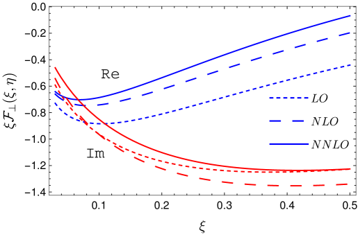
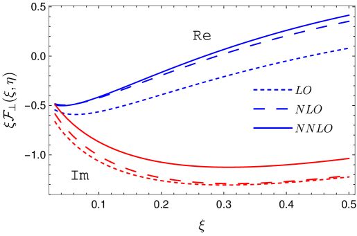
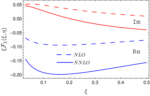
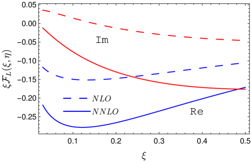
For a numerical evaluation of the convolution integrals in the $x<\xi$ region it proves to be convenient to shift the integration contour to the complex plane. We have checked that the results do not depend on the shape of the integration contour, which is a good test of numerical accuracy. The results for the transverse and the longitudinal CFFs (7) are shown in Fig. 1 and Fig. 2, respectively. We show real (blue) and imaginary (red) parts of the CFFs as a function of $\xi$ for the fixed value of $\omega=\xi/\eta=-1.63158$ (upper panels) and $\omega=\xi/\eta=-1.27273$ (lower panels). The leading-order (LO) results are shown by short dashes, and the calculation including one-loop (NLO) and two-loop corrections (NNLO) by the long dashes and solid curves, respectively.

One sees that the corrections are in general quite large (for the chosen kinematics) and have a nontrivial structure. In particular for $\mathcal{F}_{\perp}(\xi,\eta)$, the NLO (one loop) corrections are large for the real part and small for imaginary part of the CFF, whereas the NNLO (two-loop) corrections, on the contrary, are small for the real part and large for imaginary part. The NNLO corrections for $\mathcal{F}_{L}(\xi,\eta)$ are very large so that the perturbative expansion does not show any sign of convergence for this case. These features certainly call for an increase of the invariant mass of the lepton pair which, hopefully, will become possible in future experiments.

As far as the relative contributions of the three color structures (19) in the NNLO correction are concerned, the terms proportional to the QCD $\beta$-function prove to be the largest, but are partially compensated by contributions of “planar” diagrams $\sim C_{F}^{2}$. The non-planar contributions $\sim C_{F}/N_{c}$ are in all cases an order of magnitude below the planar ones.

6 Summary

Using the approach based on conformal symmetry Braun:2013tva ; Braun:2020yib we have calculated the two-loop coefficient functions in double deeply virtual Compton scattering in the $\overline{\text{MS}}$ scheme for the flavor-nonsinglet vector contributions. Analytic expressions for the coefficient functions in momentum fraction space are presented in Appendix E and in two ancillary files using different representations for the relevant generalized polylogarithms. Numerical estimates in Sect. 5 suggest that the two-loop contribution to the Compton form factors at the scale of proposed experiments is significant.

The technique developed in this work can be used to calculate the two-loop contributions to the flavor-nonsinglet coefficient functions for the correlation functions of all quark-antiquark currents with applications to, e.g., the light-cone sum rules for the pion electromagnetic and transition form factors Braun:1999uj ; Agaev:2010aq .

Acknowledgments

We thank J. Wagner and L. Szymanowski for the discussion of analytic continuation properties of the DDVCS amplitudes. This study was supported by Deutsche Forschungsgemeinschaft (DFG) through the Research Unit FOR 2926, “Next Generation pQCD for Hadron Structure: Preparing for the EIC”, project number 40824754. In addition, H.-Y.J. gratefully acknowledges support from the National Natural Science Foundation of China with Grant No. 12405114.

Appendices

Appendix A Helicity amplitudes

In this Appendix, we discuss the decomposition of the generalized Compton amplitude in terms of helicity amplitudes. It is convenient Braun:2012bg to use the photon momenta $q_{1}$, $q_{2}$ to define the longitudinal plane spanned by two light-like vectors $n^{\mu}$, $\tilde{n}^{\mu}$. In the present context we can put $\Delta^{2}=0$ and define

$\displaystyle n^{\mu}=\frac{q_{1}^{\mu}}{q_{1}^{2}}-\frac{q_{2}^{\mu}}{q_{2}^{2}}\,,\qquad\tilde{n}^{\mu}=q_{1}^{\mu}-q_{2}^{\mu}=\Delta^{\mu}\,,\qquad(n\tilde{n})=\frac{1}{2}\frac{(q_{1}^{2}-q_{2}^{2})^{2}}{q_{1}^{2}q_{2}^{2}}=\frac{2\omega^{2}}{1-\omega^{2}}.$ (A.93)

The amplitude (1) can be expanded in terms of helicity amplitudes to twist-two accuracy as follows:

$\displaystyle A^{\text{t2}}_{\mu\nu}$ $\displaystyle=\epsilon_{\mu}^{+}\epsilon_{\nu}^{-}A^{+-}+\epsilon_{\mu}^{-}\epsilon_{\nu}^{+}A^{-+}+\epsilon_{\mu}^{L}(q)\epsilon_{\nu}^{L}(q^{\prime})A^{L}=-g_{\mu\nu}^{\perp}A_{V}+\epsilon_{\mu\nu}^{\perp}A_{A}+\hat{\epsilon}_{\mu}^{L}(q_{1})\hat{\epsilon}_{\nu}^{L}(q_{2})A_{L}\,.$ (A.94)

Here

$\displaystyle g_{\mu\nu}^{\perp}=g_{\mu\nu}-\frac{n^{\mu}\tilde{n}^{\nu}+n^{\nu}\tilde{n}^{\mu}}{(n\tilde{n})},\qquad\quad\epsilon_{\mu\nu}^{\perp}=\frac{1}{(n\tilde{n})}\epsilon_{\mu\nu\alpha\beta}n^{\alpha}\tilde{n}^{\beta},$ (A.95)

$\epsilon^{\pm}_{\mu}$ are orthogonal unit vectors in the transverse plane that can be taken as transverse polarization vectors for both initial and final photons, and the longitudinal photon polarization vectors are given by

$\displaystyle\hat{\epsilon}_{L}^{\mu}(q_{1})$ $\displaystyle=\frac{1}{wQ\sqrt{1+\omega}}\Big{[}q_{1}^{\mu}-q_{2}^{\mu}(1+\omega)\Big{]}\,,$
$\displaystyle\hat{\epsilon}_{L}^{\nu}(q_{2})$ $\displaystyle=\frac{1}{wQ\sqrt{1-\omega}}\Big{[}q_{2}^{\nu}-q_{1}^{\nu}(1-\omega)\Big{]}\,.$ (A.96)

The longitudinal helicity amplitude can therefore be projected as

$\displaystyle A_{L}$ $\displaystyle=\hat{\epsilon}_{L}^{\mu}(q_{1})T_{\mu\nu}\hat{\epsilon}_{L}^{\nu}(q_{2})=-\frac{\sqrt{1-\omega^{2}}}{\omega^{2}Q^{2}}\Delta^{\mu}T_{\mu\nu}\Delta^{\nu},$ (A.97)

where we used that, since $q_{1}^{\mu}T_{\mu\nu}=T_{\mu\nu}q_{2}^{\nu}=0$, one can replace

$\displaystyle\hat{\epsilon}_{L}^{\mu}(q_{1})\mapsto\frac{\sqrt{1+\omega}}{\omega Q}\Delta^{\mu},\qquad\quad\hat{\epsilon}_{L}^{\nu}(q_{2})\mapsto-\frac{\sqrt{1-\omega}}{\omega Q}\Delta^{\nu}.$ (A.98)

Comparing these expressions with the the conventional decomposition in terms of (generalized) Compton form factors in (5), we get

$\displaystyle A_{V}$ $\displaystyle=\mathcal{F}_{1}=\mathcal{F}_{\perp}\,,\qquad\quad A_{L}=-\sqrt{1-\omega^{2}}\mathcal{F}_{L}\,.$ (A.99)

Note that the longitudinal CFF $\mathcal{F}_{L}$ does not vanish for $\omega=\pm 1$, but it does not contribute to DVCS and TCS thanks to the $\sqrt{1-\omega^{2}}$ prefactor.

Appendix B The $\widehat{\mathcal{K}}_{\perp}$ kernel

Here, we present the eigenvalues of the $\widehat{K}_{\perp}$ kernels employed in Sect. 4:

$\displaystyle\widehat{\mathcal{K}}_{\perp}^{(2,\beta)}(N)=\left(2\zeta_{2}+\frac{5}{9}\right)S_{1}-\left(\zeta_{2}+\frac{10}{9}\right)\frac{1}{N(N+1)}+2\zeta_{3}-\frac{65}{6}\zeta_{2}+\frac{45}{8},$
$\displaystyle\widehat{\mathcal{K}}^{(2,P)}_{\perp}(N)=$
$\displaystyle=\frac{1}{2}\left(\mathcal{K}_{\perp}^{(1)}(N)\right)^{2}+4\zeta_{2}(\bar{\gamma}^{(1)}_{N})^{2}+4\zeta_{3}\left(11+\frac{12}{N(N+1)}\right)-64\zeta_{3}S_{1}-8\zeta_{2}S_{1}^{2}+\frac{6S_{-2}}{N(N+1)}$
$\displaystyle\quad+\frac{{2S_{1}^{2}}}{N(N+1)}+12\zeta_{2}\left(-{1}+\frac{{2}}{3N(N+1)}\right)S_{1}+\left(\frac{149}{9}-\frac{8}{N(N+1)}-\frac{{2}}{N^{2}(N+1)^{2}}\right)S_{1}$
$\displaystyle\quad+\frac{11}{8}+\frac{11}{3}\zeta_{2}+8\zeta_{2}^{2}-\frac{19}{9N(N+1)}-\frac{{16}}{N^{2}(N+1)^{2}}-\frac{{2}}{N^{3}(N+1)^{3}}\,,$
$\displaystyle\widehat{\mathcal{K}}^{(2,NP)}_{\perp}(N)=$
$\displaystyle=-12S_{-2}^{2}-8S_{-4}+4\Big{(}2S_{1,3}-S_{4}\Big{)}-\frac{12S_{3}}{N(N+1)}+\frac{24\left(S_{-3}-2S_{1,-2}\right)}{N(N+1)}+\frac{16S_{1}S_{-2}}{N(N+1)}$
$\displaystyle\quad+\left(\frac{36}{N^{2}(N+1)^{2}}+\frac{24}{(N-2)(N+3)}+\frac{52}{N(N+1)}+8\right)S_{-2}$
$\displaystyle\quad+\left(-\frac{8}{N^{3}(N+1)^{3}}-\frac{8}{N^{2}(N+1)^{2}}-\frac{{10}}{N(N+1)}+{\frac{70}{9}}\right)S_{1}$
$\displaystyle\quad-\frac{{68}}{9N(N+1)}+\frac{18}{(N-2)(N+3)}-\frac{35}{4}+\left(\frac{50}{N(N+1)}+54\right)\zeta_{3}$
$\displaystyle\quad-4\zeta_{2}^{2}-36\zeta_{3}S_{1}-\frac{12\zeta_{2}S_{1}}{N(N+1)}+\zeta_{2}\left(\frac{8}{N^{2}(N+1)^{2}}+\frac{4}{N(N+1)}-\frac{20}{3}\right)\,.$ (B.100)

Appendix C $SL(2)$-invariant kernels

We collect here the invariant kernels and their eigenvalues used in Sect. 4. Let

$\displaystyle\mathrm{M}_{n}[\omega]=\int_{0}^{1}d\alpha\int_{0}^{\bar{\alpha}}\!d\beta\,\omega(\tau)(1-\alpha-\beta)^{n-1}\,,\qquad\tau=\frac{\alpha\beta}{\bar{\alpha}\bar{\beta}}\,,\qquad\bar{\tau}=1-\tau\,,$ (C.101)

where $n$ is even. One obtains

$\displaystyle\mathcal{H}_{+}$ $\displaystyle:\qquad\mathrm{M}_{n}[1]=\frac{1}{n(n+1)}\,,\qquad$ $\displaystyle\mathcal{H}_{++}:\qquad\mathrm{M}_{n}[-\ln\bar{\tau}]=\frac{1}{n^{2}(n+1)^{2}}\,,$
$\displaystyle\mathcal{H}_{1,+}$ $\displaystyle:\qquad\mathrm{M}_{n}[-\ln\tau]=\frac{2S_{1}(n)}{n(n+1)}\,,\qquad$ $\displaystyle\mathcal{H}_{-2}:\qquad\mathrm{M}_{n}[\bar{\tau}]=2S_{-2}(n)+\zeta_{2}\,,$
$\displaystyle\mathcal{H}_{-2,+}$ $\displaystyle:\qquad\mathrm{M}_{n}[\operatorname{Li}_{2}(\tau)]=\frac{2S_{-2}(n)+\zeta_{2}}{n(n+1)}\,,\qquad$ $\displaystyle\mathcal{H}_{3}:\qquad\mathrm{M}_{n}\left[\frac{\bar{\tau}}{2\tau}\ln\bar{\tau}\right]=S_{3}(n)-\zeta_{3}\,,$ (C.102)

and

$\displaystyle\mathcal{H}_{-3}:\qquad\mathrm{M}_{n}\left[-\bar{\tau}\ln\bar{\tau}\right]=2S_{-3}(n)-4S_{1,-2}(n)-2\zeta_{2}S_{1}(n)+\zeta_{3}\,,$
$\displaystyle\mathcal{H}_{-4}:\qquad\mathrm{M}_{n}\left[\bar{\tau}\left(\operatorname{Li}_{2}(\tau)+\frac{1}{2}\ln^{2}\bar{\tau}\right)\right]=2S_{-4}(n)+\frac{7}{10}\zeta_{2}^{2}\,,$
$\displaystyle\mathcal{H}_{1,3}:\qquad\mathrm{M}_{n}\left[\frac{\bar{\tau}}{4\tau}\left(\operatorname{Li}_{2}(\tau)+\frac{1}{2}\ln^{2}\bar{\tau}\right)\right]=S_{1,3}(n)-\frac{1}{2}S_{4}(n)-\zeta_{3}S_{1}(n)+\frac{3}{10}\zeta_{2}^{2}\,,$
$\displaystyle\mathcal{H}_{\mathrm{s}ing}:\qquad\mathrm{M}_{n}\left[\frac{\tau^{2}\!+\!4\tau\!+\!1}{(\tau-1)^{2}}\big{[}\operatorname{Li}_{2}(\tau)-\zeta_{2}\big{]}+3\Big{(}\frac{\tau\!+\!1}{\tau\!-\!1}\Big{)}\ln(1\!-\!\tau)-\frac{3}{2}\frac{3\tau+1}{(\tau-1)}\right]=\frac{2S_{-2}(n)+3/2}{(n-2)(n+3)}.$ (C.103)

Appendix D Restoring the scale dependence

In this Appendix, we provide details for the restoration of the scale dependence of the coefficient functions mentioned in Sect. 3.3. The scale-dependent terms $\sim\ln Q/\mu,\ln^{2}Q/\mu$ in the CFs are completely fixed by the renormalization group equations. Since the evolution kernel in the $\overline{\rm MS}$ scheme does not depend on $\epsilon$, $\mathbb{H}(a_{s},\epsilon)=\mathbb{H}(a_{s})$, in a generic $d$-dimensional theory

$\displaystyle\Big{(}\mu\partial_{\mu}+\beta(a_{s},\epsilon)\partial_{a_{s}}\Big{)}C\left(Q^{2}/\mu^{2},a_{s},\epsilon\right)=C\left(Q^{2}/\mu^{2},a_{s},\epsilon\right)\otimes\mathbb{H}(a_{s})\,,$ (D.104)

where

$\displaystyle C\otimes\mathbb{H}=\int_{-1}^{1}dx^{\prime}\,C(x^{\prime})\,\mathbb{H}(x^{\prime},x)\,.$ (D.105)

Solving this equation one obtains Braun:2020yib

$\displaystyle C(\sigma,a_{s},\epsilon)$ $\displaystyle=\Big{(}C^{(0)}+a_{s}C^{(1)}(\epsilon)+a_{s}^{2}C^{(2)}(\epsilon)+\ldots\Big{)}\otimes\Big{(}1-\frac{1}{2}\ln\sigma\,\mathbb{H}(a_{s})+\frac{1}{8}\ln^{2}\!\sigma\,\mathbb{H}^{2}(a_{s})+\ldots\Big{)}\,$
$\displaystyle\quad-\beta(a_{s},\epsilon)\left(-\frac{1}{2}C_{1}(\epsilon)\,\ln\sigma+\frac{1}{8a_{s}}\ln^{2}\sigma\,C_{0}\otimes\mathbb{H}(a_{s})\right)+O(a_{s}^{3},a_{s}^{2}\epsilon,a_{s}\epsilon^{2})\,.$ (D.106)

Here $\sigma=Q^{2}/\mu^{2}$ and $C^{(0)},C^{(1)}(\epsilon),C^{(2)}(\epsilon)$ are the CFs in $d$ dimensions (21) at $\mu^{2}=Q^{2}$, alias $\sigma=1$. Note that the contribution in the second line vanishes at the critical point, $\beta(a_{s},\epsilon_{\ast})=0$. For the physical case $d=4$ one obtains

$\displaystyle C(\sigma,a_{s},\epsilon=0)$ $\displaystyle=C^{(0)}+a_{s}\biggl{(}C^{(1)}_{\ast}-\frac{1}{2}\ln\sigma\,C^{(0)}\otimes\mathbb{H}^{(1)}\biggr{)}+a_{s}^{2}\biggl{\{}C_{2}^{(*)}+\beta_{0}C^{(1,1)}$
$\displaystyle\quad-\frac{1}{2}\ln\sigma\biggl{[}C^{(0)}\!\otimes\mathbb{H}^{(2)}+2C^{(1)}\!\otimes\Big{(}\beta_{0}+\frac{1}{2}\mathbb{H}^{(1)}\Big{)}\biggr{]}$
$\displaystyle\quad+\frac{1}{4}\ln^{2}\!\sigma\,C^{(0)}\!\otimes\mathbb{H}^{(1)}\Big{(}\beta_{0}+\frac{1}{2}\mathbb{H}^{(1)}\Big{)}\!\biggr{\}}\,,$ (D.107)

where the CFs in $d=4$ are related to the ones at the critical point as $C^{(1)}(\epsilon=0)=C^{(1)}_{\ast}$ and $C^{(2)}(\epsilon=0)=C_{\ast}^{(2)}+\beta_{0}C^{(1,1)}$, see Eq. (25).

Appendix E Two-loop coefficient functions

In this Appendix, we present explicit results for the two-loop coefficient functions discussed in Sect.  4. We express our results in terms of multiple polylogarithms

$\displaystyle\operatorname{Li}_{n_{1},\ldots,n_{r}}(z_{1},\ldots,z_{r})=\sum_{0<k_{1}<\ldots<k_{r}}\frac{z_{1}^{k_{1}}\cdots z_{r}^{k_{r}}}{k_{1}^{n_{1}}\cdots k_{r}^{n_{r}}}\,,$ (E.108)

where the depth $r$ denotes the number of summations. We note that this convention follows those of Refs. Goncharov:1998kja ; Borwein:1999js and the HyperInt package Panzer:2014caa , whereas the order of subscripts and arguments need to be reversed to match the conventions of Ginac’s $\operatorname{Li}$ functions Vollinga:2004sn . The $\operatorname{Li}$ functions can easily be converted into $\operatorname{G}$ function notation (86) and vice versa. Threshold expansions of our results are presented in Appendix F below.

E.1 Longitudinal CF

As was discussed in Sect. 3, the difference between the critical and four dimensional CFs at two loops, $C_{L}^{(2)}(z,\omega)-C_{*,L}^{(2)}(z,\omega)=\beta C_{L}^{(11)}(z,\omega)$ comes from the $\epsilon$-expansion of the one-loop CF in $d=4-2\epsilon$ dimensions. Taking this contribution into account and adding the RG logarithms as explained in App. D, we write the two-loop longitudinal CF using the notations in Eqs. (2),(19),(20). The $A_{L}$ -type contributions all vanish. The terms $\sim\ln(Q^{2}/\mu^{2})$ in the $B_{L}$-functions corresponding to the different color structures, Eq. (19), take the following form:

$\displaystyle B_{L,\ln}^{(2,\beta)}(z,w)$ $\displaystyle=-2\mathrm{L}_{1}(z,w)\,,$
$\displaystyle B_{L,\ln}^{(2,P)}(z,w)$ $\displaystyle=\mathrm{L}_{2}(z,-w)-\mathrm{L}_{2}(w,-w)+\mathrm{L}_{1}(z,w)\left(\mathrm{L}_{1}(z,-w)+\frac{3}{2}\right),$
$\displaystyle B_{L,\ln}^{(2,NP)}(z,w)$ $\displaystyle=0\,.$ (E.109)

The remaining contributions are:

$\bullet$  Terms $\sim\beta_{0}C_{F}$:

$\displaystyle B_{L}^{(2,\beta)}(z,w)$ $\displaystyle=2\,\mathrm{L}_{2}(z,w)+\frac{13}{3}\mathrm{L}_{1}(z,w)+\Big{[}-\ln^{2}(1-z)+\ln^{2}(1-w)+2\mathrm{L}_{1}(z,w)\Big{]}\,.$ (E.110)

The terms in square brackets in Eq. (E.110) originate from $C^{(11)}$.

$\bullet$  Planar contributions $\sim C_{F}^{2}$:

$\displaystyle B_{L}^{(2,P)}(z,w)$ $\displaystyle=4\biggl{\{}\mathrm{L}_{12}(z,w)+\mathrm{L}_{3}(z,-w)-\mathrm{L}_{3}(w,-w)+\Big{(}\mathrm{L}_{2}(z,-w)-\mathrm{L}_{2}(w,-w)\Big{)}\ln(1+w)$
$\displaystyle\quad+\frac{1}{3}\Big{(}\ln^{3}(1-z)-\ln^{3}(1-w)\Big{)}-\frac{3}{2}\mathrm{L}_{2}(z,w)+\frac{1}{4}\Big{(}\ln^{2}(1-z)-\ln^{2}(1-w)\Big{)}$
$\displaystyle\quad-\frac{1}{2}\left(\ln^{2}(1+w)+\ln^{2}(1-w)-\ln(1-w^{2})+\frac{47}{6}\right)\mathrm{L}_{1}(z,w)\biggr{\}}.$ (E.111)

$\bullet$  Non-planar contributions $\sim C_{F}/N_{c}$ are considerably more complicated:

$\displaystyle B_{L}^{(2,NP)}(z,w)~{}=$
$\displaystyle\quad=4\biggl{\{}\mathrm{L}_{2}(z,w)\Big{[}\mathrm{L}_{2}(z,-w)+\mathrm{L}_{2}(-z,w)\Big{]}+\widehat{\,\mathrm{M}}_{22}(-z,-w)-\widehat{\,\mathrm{M}}_{22}(-w,-z)+6\,\mathrm{L}_{112}(z,w)$
$\displaystyle\qquad\quad+\mathrm{L}_{1}(z,w)\left[\widehat{L}_{3}(z,w)+4\mathrm{L}_{12}(z,w)-6\zeta_{3}\right]-\frac{1}{2}\Big{[}\mathrm{L}_{1}^{2}(z,-w)-\mathrm{L}_{1}^{2}(w,-w)\Big{]}\mathrm{L}_{2}(-z,w)$
$\displaystyle\qquad\quad+\mathrm{L}_{2}(z,w)\Big{[}\mathrm{L}^{2}_{1}(z,w)+\frac{1}{2}\mathrm{L}_{1}^{2}(w,-w)\Big{]}+\mathrm{L}_{1}(-z,-w)\mathrm{L}_{2}(z,w)+\mathrm{L}_{1}(-z,w)\mathrm{L}_{2}(z,-w)$
$\displaystyle\qquad\quad-\frac{1}{6}\mathrm{L}^{3}_{1}(w,-w)\mathrm{L}_{1}(z,w)-\frac{1}{4}\mathrm{L}^{2}_{1}(w,-w)\mathrm{L}_{1}(z,-z)-\mathrm{L}_{1}(z,-z)\mathrm{L}_{1}(z,w)+\frac{5}{3}\mathrm{L}_{1}(z,w)\biggr{\}}$
$\displaystyle\qquad\quad-\frac{2(w^{2}-3)}{w^{2}}\left\{\mathrm{L}_{1}(-z,-w)\mathrm{L}_{2}(z,w)+\mathrm{L}_{1}(-z,w)\mathrm{L}_{2}(z,-w)-\frac{1}{4}\mathrm{L}^{2}_{1}(w,-w)\mathrm{L}_{1}(z,-z)\right\}$
$\displaystyle\quad\quad-\frac{12}{w}\left\{\mathrm{L}_{2}(z,-w)+\frac{1}{4}\mathrm{L}^{2}_{1}(w,-w)-\frac{1}{2}(w-2)\mathrm{L}_{1}(z,w)\right\}$
$\displaystyle\quad\quad+6(w-z)\Biggl{\{}\frac{z}{w^{4}}(w^{2}-3)\biggl{[}\widehat{D}_{L}(w)-\mathrm{M}_{22}(z,w)+\frac{1}{2}\mathrm{L}_{2}(z,w)\left(\mathrm{L}_{2}(-z,w)+\frac{1}{2}\mathrm{L}^{2}_{1}(w,-w)\right)$
$\displaystyle\qquad\qquad\qquad-\mathrm{L}_{4}(-z,-w)+\mathrm{L}_{2}(z,w)\mathrm{L}_{2}(-1,-w)-\frac{1}{4}\mathrm{L}_{1}(w,-w)\left[\widehat{L}_{3}(z,w)+6\zeta_{3}\right]$
$\displaystyle\qquad\qquad\qquad-\frac{2w}{z}\biggl{(}\mathrm{L}_{1}(z,-w)\mathrm{L}_{2}(-z,w)+\!\frac{1}{4}\mathrm{L}^{2}_{1}(w,-w)\mathrm{L}_{1}(z,w)\biggr{)}\biggr{]}$
$\displaystyle\qquad\qquad\qquad+\frac{6z}{w^{3}}\biggl{[}\frac{1}{4}\widehat{L}_{3}(z,w)-\frac{1}{2}\widehat{L}_{12}(z,w)-\frac{3}{2}\zeta_{3}-\left(\frac{1}{4}\mathrm{L}^{2}_{1}(w,-w)+\mathrm{L}_{2}(-z,-w)\right)\mathrm{L}_{1}(z,w)\biggr{]}$
$\displaystyle\qquad\qquad\qquad+2\frac{w-3}{w^{2}}\mathrm{L}_{2}(z,w)-\frac{2}{w}\mathrm{L}_{1}(z,w)\Biggr{\}}.$ (E.112)

Here,

$\displaystyle\widehat{D}_{L}(w)$ $\displaystyle=-\frac{1}{24}\ln^{3}w_{+}\Big{(}\ln w_{+}-4\ln w_{-}\Big{)}-3\operatorname{Li}_{13}\left(w_{-}\right)+6\operatorname{Li}_{4}\left(w_{-}\right)$
$\displaystyle\quad-\Big{(}\ln w_{+}+2\ln w_{-}\Big{)}\operatorname{Li}_{3}\left(w_{-}\right)-\frac{1}{2}\zeta_{2}\ln^{2}w_{-}+2\zeta_{3}\ln w_{-}\,,$ (E.113)

where $w_{\pm}=(1\pm w)/2$, and we use the following notation:

$\displaystyle\mathrm{L}_{\vec{n}}(z,w)=\begin{cases}\ln\left(\frac{1-z}{1-w}\right)&\vec{n}=1\\ \operatorname{Li}_{\vec{n}}\left(1,\dots,1,\frac{z-w}{1-w}\right)&\vec{n}\neq 1\end{cases}$ (E.114)

and

$\displaystyle\mathrm{M}_{22}(z,w)=\operatorname{Li}_{22}\left(\frac{z-w}{1-w},\frac{w-1}{w+1}\right)\,,$ $\displaystyle\widehat{\,\mathrm{M}}_{22}(z,w)=\operatorname{Li}_{22}\left(\frac{1+z}{1+w},\frac{z+w}{1+z}\right)\,,$ (E.115)

where $\operatorname{Li}_{\vec{n}}(\vec{z})$ are the multiple polylogarithms defined in (E.108). The hatted letters stand for the following combinations

$\displaystyle\widehat{L}_{3}(z,w)$ $\displaystyle=\mathrm{L}_{3}(z^{2},w^{2})-\mathrm{L}_{3}(z,w)-\mathrm{L}_{3}(-z,w)-\mathrm{L}_{3}(z,-w)-\mathrm{L}_{3}(-z,-w),$
$\displaystyle\widehat{L}_{12}(z,w)$ $\displaystyle=\mathrm{L}_{12}(z^{2},w^{2})-\mathrm{L}_{12}(z,w)-\mathrm{L}_{12}(-z,w)-\mathrm{L}_{12}(z,-w)-\mathrm{L}_{12}(-z,-w).$ (E.116)

All $B_{L}$-functions are regular at $z=w$. Moreover, $B_{L}^{(2,\beta)}(w,w)=B_{L}^{(2,P)}(w,w)=0$, and for the non-planar contribution the following identity holds: $B_{L}^{(2,NP)}(w,w)-B_{L}^{(2,NP)}(-w,-w)=0$. It can also be checked that $B^{(2,NP)}_{L}(z,w)$ is regular at the point $w=0$. Thus the longitudinal CF is a real analytic function in the whole Euclidean domain $-1<z<1$, $-1<w<1$ with logarithmic branching cuts outside this region.

E.2 Transverse CF

The resulting expression for the transverse CF can be brought to the form in Eqs. (2), (19), (20). The double logarithmic contributions $\sim\ln^{2}(Q^{2}/\mu^{2})$ are rather simple in this case too:

$\displaystyle A^{(2,\beta)}_{\perp,\ln^{2}}(z,w)$ $\displaystyle=-\mathrm{L}_{1}(z,w)-\frac{3}{4}\,,$
$\displaystyle B^{(2,\beta)}_{\perp,\ln^{2}}(z,w)$ $\displaystyle=\frac{1}{2}({1+w})\,\mathrm{L}_{1}(z,w)\,,$
$\displaystyle A^{(2,P)}_{\perp,\ln^{2}}(z,w)$ $\displaystyle=4\mathrm{L}_{2}(z,w)+4\mathrm{L}_{1}^{2}(z,w)-\mathrm{L}_{1}^{2}(w,-w)+6\mathrm{L}_{1}(z,w)+\frac{9}{4}\,,$
$\displaystyle B^{(2,P)}_{\perp,\ln^{2}}(z,w)$ $\displaystyle=(1+w)\Big{[}\mathrm{L}_{2}(w,-w)\!-\!\mathrm{L}_{2}(z,-w)\!-\!2\mathrm{L}_{1}(z,w)\Big{(}\mathrm{L}_{1}(z,-w)+\frac{3}{2}\Big{)}-\mathrm{L}_{1}(-z,-w)\Big{]},$
$\displaystyle A^{(2,NP)}_{\perp,\ln^{2}}(z,w)$ $\displaystyle=B^{(2,NP)}_{\perp,\ln^{2}}(z,w)=0\,.$ (E.117)

For the single-logarithmic contributions $\sim\ln(Q^{2}/\mu^{2})$ we obtain

$\displaystyle A^{(2,\beta)}_{\perp,\ln}(z,w)$ $\displaystyle=2\mathrm{L}_{2}(z,w)-\ln^{2}(1-z)+\ln^{2}(1-w)+\frac{29}{6}\mathrm{L}_{1}(z,w)-\frac{3}{2}\ln(1-w)+\frac{19}{4},$
$\displaystyle B^{(2,\beta)}_{\perp,\ln}(z,w)$ $\displaystyle=\frac{1+w}{2}\Big{[}\ln^{2}(1-z)-\ln^{2}(1-w)-2\mathrm{L}_{2}(z,w)-\frac{19}{3}\mathrm{L}_{1}(z,w)-\mathrm{L}_{1}(-z,-w)\Big{]},$
$\displaystyle A^{(2,P)}_{\perp,\ln}(z,w)$ $\displaystyle=8\mathrm{L}_{3}(z,w)+4\mathrm{L}_{1}^{3}(z,w)+4\Big{[}2\ln(1-w)-3\Big{]}\mathrm{L}_{2}(z,w)$
$\displaystyle\quad+\Big{[}4\ln(1-w^{2})-3\Big{]}\mathrm{L}_{1}^{2}(z,w)-\mathrm{L}_{1}(z,w)\Big{[}4\mathrm{L}_{1}^{2}(w,-w)-6\ln(1-w^{2})+\frac{103}{6}\Big{]}$
$\displaystyle\quad-\frac{47}{4}+\frac{1}{3}\ln^{3}(1-w^{2})-\frac{8}{3}\ln^{3}(1-w)+\frac{9}{2}\ln(1-w),$
$\displaystyle B^{(2,P)}_{\perp,\ln}(z,w)$ $\displaystyle=-2(1+w)\biggl{\{}\mathrm{L}_{12}(z,w)+\mathrm{L}_{3}(z,-w)+\mathrm{L}_{1}^{3}(z,w)-\frac{3}{2}\mathrm{L}_{2}(z,w)-\frac{3}{2}\mathrm{L}_{2}(-z,w)$
$\displaystyle\quad+\big{(}\ln(1+w)-1\big{)}\mathrm{L}_{2}(z,-w)-\frac{1}{2}\Big{(}\ln(1+w)-5\ln(1-w)+3\Big{)}\mathrm{L}_{1}^{2}(z,w)$
$\displaystyle\quad-\mathrm{L}_{1}^{2}(-z,-w)-\frac{1}{2}\mathrm{L}_{1}(z,w)\left(\ln^{2}(1-w^{2})-4\ln^{2}(1-w)-6\ln(1+w)+\frac{65}{6}\right)$
$\displaystyle\quad-\frac{1}{2}\mathrm{L}_{1}(-z,-w)\left(\ln(1+w)-3\ln(1-w)+\frac{19}{2}\right)$
$\displaystyle\quad-\mathrm{L}_{3}(w,-w)-\big{(}\ln(1+w)-1\big{)}\mathrm{L}_{2}(w,-w)+\frac{3}{2}\mathrm{L}_{2}(-w,w)\biggr{\}},$
$\displaystyle A^{(2,NP)}_{\perp,\ln}(z,w)$ $\displaystyle=-2\widehat{L}_{3}(z^{2},w^{2})+4\widehat{L}_{12}(z,w)+8\mathrm{L}_{1}(z,w)\mathrm{L}_{2}(-z,-w)+2\mathrm{L}_{1}^{2}(w,-w)\mathrm{L}_{1}(z,w)$
$\displaystyle\quad+\frac{8}{3}\mathrm{L}_{1}(z,w)+\frac{1}{2},$
$\displaystyle B^{(2,NP)}_{\perp,\ln}(z,w)$ $\displaystyle=4w\Big{(}\mathrm{P}_{12}(z,w)+\mathrm{L}_{3}(z,w)-\frac{1}{2}\widehat{L}_{12}(z,w)\Big{)}-2(1-w)\mathrm{L}_{1}(w,-w)\mathrm{L}_{2}(z,-w)$
$\displaystyle\quad-2(1+w)\mathrm{L}_{1}(z,w)\Big{(}\mathrm{L}_{2}(-z,-w)+\mathrm{L}_{2}(-z,w)+\frac{1}{2}\mathrm{L}_{1}^{2}(w,-w)\Big{)}$
$\displaystyle\quad-\left(\frac{10}{3}-\frac{2}{3}w\right)\mathrm{L}_{1}(z,w)-2w\Big{(}\mathrm{L}_{12}(w,-w)+\mathrm{L}_{12}(-w,w)\Big{)}$
$\displaystyle\quad+2(1-w)\mathrm{L}_{1}(w,-w)\mathrm{L}_{2}(w,-w).$ (E.118)

The function $\mathrm{P}_{12}$ is defined in Eq. (E.2).

The remaining contributions are:

$\bullet$  Terms $\sim\beta_{0}C_{F}$:

$\displaystyle A_{\perp}^{(2,\beta)}(z,w)$ $\displaystyle=\mathrm{L}_{3}(z,w)-2\,\mathrm{L}_{12}(z,w)+2\,\mathrm{L}_{2}(z,w)\left(\ln(1-w)-\frac{7}{3}\right)-\frac{3}{4}\zeta_{2}-\frac{25}{48}$
$\displaystyle\quad+\frac{5}{3}\biggl{(}\ln^{2}(1-z)-\ln^{2}(1-w)\biggr{)}-\left(\frac{121}{36}+\zeta_{2}\right)\mathrm{L}_{1}(z,w)+\frac{1}{4}\ln(1-w)$
$\displaystyle\quad+\biggl{\{}-\frac{1}{3}\bigl{[}\ln^{3}(1-z)-\ln^{3}(1-w)\bigr{]}+\frac{3}{4}\bigl{[}\ln^{2}(1-z)-2\ln^{2}(1-w)\bigr{]}$
$\displaystyle\quad+\zeta_{2}\mathrm{L}_{1}(z,w)-\frac{7}{2}\ln(1-z)+8\ln(1-w)-9+\frac{3}{4}\zeta_{2}\biggr{\}},$ (E.119a)
$\displaystyle B_{\perp}^{(2,\beta)}(z,w)$ $\displaystyle=\frac{1+w}{2}\biggl{[}2\,\mathrm{L}_{12}(z,w)-\mathrm{L}_{3}(z,w)-2\,\mathrm{L}_{2}(z,w)\left[\ln(1-w)-\frac{10}{3}\right]+\frac{31}{9}\mathrm{L}_{1}(z,w)$
$\displaystyle\quad+\zeta_{2}\mathrm{L}_{1}(z,w)\biggr{]}-\frac{w+4}{3}\bigl{[}\ln^{2}(1-z)-\ln^{2}(1-w)\bigr{]}-2\mathrm{L}_{2}(z,w)+\frac{1}{6}\mathrm{L}_{1}(z,w)$
$\displaystyle\quad+\biggl{\{}(1+w)\biggl{(}\frac{1}{6}\mathrm{L}_{1}^{3}(z,w)+\frac{1}{2}\ln(1-w)\mathrm{L}_{1}^{2}(z,w)-\frac{3}{4}\biggl{[}\mathrm{L}_{1}^{2}(z,w)+\mathrm{L}_{1}^{2}(-z,-w)\biggr{]}\biggr{)}$
$\displaystyle\quad-\mathrm{L}_{1}(z,w)\left(w\left[3\ln(1-w)-6\right]+\frac{1+w}{2}\zeta_{2}-2-\frac{1}{2}(1+w)\ln^{2}(1-w)\right)\biggr{\}}.$ (E.119b)

The terms in the curly brackets in Eq. (E.119) originate from the $\epsilon$-correction term $C^{(1,1)}$, see Eq. (25).

$\bullet$  Planar contributions $\sim C_{F}^{2}$:

$\displaystyle A_{\perp}^{(2,P)}(z,w)=$
$\displaystyle=4\biggl{\{}\frac{701}{192}+\frac{9}{2}\zeta_{3}+\mathrm{L}_{4}(z,w)+\mathrm{L}_{13}(z,w)+5\,\mathrm{L}_{112}(z,w)+\mathrm{L}_{1}(z,w)\Big{(}\mathrm{L}_{3}(z,w)+2\mathrm{L}_{12}(z,w)\Big{)}$
$\displaystyle\quad-\frac{3}{2}\mathrm{L}_{12}(z,w)+\left(2\ln(1-w)-\frac{9}{4}\right)\mathrm{L}_{3}(z,w)+\frac{1}{4}\left[\ln^{2}(1-z)-\ln^{2}(1-w)\right]^{2}$
$\displaystyle\quad-\frac{1}{16}\left[\ln^{2}(1-w)-\ln^{2}(1+w)\right]^{2}-\frac{3}{4}\Big{[}\ln^{2}(1-z)-\ln^{2}(1-w)\Big{]}\Big{(}\mathrm{L}_{1}(z,w)-\ln(1+w)\Big{)}$
$\displaystyle\quad+\left(\ln^{2}(1-w)-3\ln(1-w)+\frac{37}{12}\right)\mathrm{L}_{2}(z,w)-\frac{9}{4}\ln(1-w)\left[\ln(1-z)-\frac{1}{2}\ln(1+w)\right]$
$\displaystyle\quad-\frac{49}{48}\ln^{2}(1-z)+\frac{65}{24}\ln^{2}(1-w)+\left(6\zeta_{3}+\frac{167}{144}\right)\mathrm{L}_{1}(z,w)-\frac{47}{16}\ln(1-w)\biggr{\}}\,,$ (E.120a)
$\displaystyle B_{\perp}^{(2,P)}(z,w)=$
$\displaystyle=(1+w)\biggl{\{}-\mathrm{L}_{1}(z,w)\Big{[}\mathrm{L}_{3}(z,w)+2\mathrm{L}_{12}(z,w)\Big{]}-3\mathrm{L}_{13}(z,w)-3\mathrm{L}_{112}(z,w)+\frac{3}{2}\mathrm{L}_{3}(z,w)$
$\displaystyle\quad-\ln(1-w)\Big{[}2\mathrm{L}_{12}(z,w)-3\mathrm{L}_{2}(z,w)\Big{]}-\frac{8}{3}\mathrm{L}_{2}(z,w)-\mathrm{L}_{4}(z,-w)-\mathrm{L}_{13}(z,-w)$
$\displaystyle\quad-\mathrm{L}_{1}(z,-w)\Big{[}\mathrm{L}_{3}(z,-w)+2\mathrm{L}_{12}(z,-w)\Big{]}-5\mathrm{L}_{112}(z,-w)-2\ln(1+w)\mathrm{L}_{3}(z,-w)$
$\displaystyle\quad-\ln^{2}(1+w)\mathrm{L}_{2}(z,-w)+\mathrm{L}_{12}(z,-w)-\frac{1}{2}\Big{[}\ln^{2}(1-z)-\ln^{2}(1-w)\Big{]}\Big{[}\ln^{2}(1-z)$
$\displaystyle\quad-\ln^{2}(1+w)+3\ln(1-w^{2})\Big{]}-12\zeta_{3}\mathrm{L}_{1}(z,w)+\frac{1}{2}\mathrm{L}_{3}(-z,w)-\mathrm{L}_{1}(-z,-w)\mathrm{L}_{2}(-z,-w)$
$\displaystyle\quad-\mathrm{L}_{1}(-z,w)\mathrm{L}_{2}(-z,w)-3\mathrm{L}_{12}(-z,w)+\frac{5}{2}\Big{[}\mathrm{L}_{3}(z,-w)+\mathrm{L}_{3}(-z,w)\Big{]}$
$\displaystyle\quad+2\Big{[}\ln^{3}(1-z)-\ln^{3}(1-w)\Big{]}+\frac{2}{3}\big{[}\ln^{3}(1+z)-\ln^{3}(1+w)\Big{]}+2\ln(1+w)\mathrm{L}_{2}(z,-w)$
$\displaystyle\quad+\Big{(}3\ln(1-w)-1\Big{)}\mathrm{L}_{2}(-z,w)-\frac{5}{2}\Big{[}(\mathrm{L}_{2}(z,-w)+\mathrm{L}_{2}(-z,w)+\frac{1}{2}\mathrm{L}_{1}^{2}(w,-w)\Big{]}$
$\displaystyle\quad-3\Big{[}\mathrm{L}_{2}(z,w)+\mathrm{L}_{2}(-z,-w)\Big{]}-\frac{3}{2}\left[\ln^{2}(1-w)+\ln^{2}(1+w)\right]\Big{[}\mathrm{L}_{1}(z,w)+\mathrm{L}_{1}(-z,-w)\Big{]}$
$\displaystyle\quad+\frac{1}{2}\ln(1+w)\mathrm{L}_{1}(z,w)+\frac{1}{2}\ln(1-w)\mathrm{L}_{1}(-z,-w)+\frac{7}{6}\Big{[}\ln^{2}(1-z)-\ln^{2}(1-w)\Big{]}$
$\displaystyle\quad+\frac{3}{2}\Big{[}\ln^{2}(1+z)-\ln^{2}(1+w)\Big{]}+\ln(1-w^{2})\Big{[}4\mathrm{L}_{1}(z,w)+3\mathrm{L}_{1}(-z,-w)\Big{]}$
$\displaystyle\quad-\frac{295}{36}\mathrm{L}_{1}(z,w)-\frac{223}{12}\mathrm{L}_{1}(-z,-w)-\widehat{D}_{\perp}(w)\biggr{\}},$ (E.120b)

where

$\displaystyle\widehat{D}_{\perp}(w)$ $\displaystyle=-\mathrm{L}_{4}(w,-w)-\mathrm{L}_{1}(w,-w)\mathrm{L}_{3}(w,-w)-\mathrm{L}_{13}(w,-w)-2\mathrm{L}_{1}(w,-w)\mathrm{L}_{12}(w,-w)$
$\displaystyle\quad-5\mathrm{L}_{112}(w,-w)-2\ln(1+w)\mathrm{L}_{3}(w,-w)-\ln^{2}(1+w)\mathrm{L}_{2}(w,-w)+\mathrm{L}_{12}(w,-w)$
$\displaystyle\quad-\mathrm{L}_{1}(-w,w)\mathrm{L}_{2}(-w,w)-3\mathrm{L}_{12}(-w,w)+\frac{1}{2}\mathrm{L}_{3}(-w,w)+3\ln(1-w)\mathrm{L}_{2}(-w,w)$
$\displaystyle\quad-\mathrm{L}_{2}(-w,w)+\frac{5}{2}(\mathrm{L}_{3}(w,-w)+\mathrm{L}_{3}(-w,w))+2\ln(1+w)\mathrm{L}_{2}(w,-w).$ (E.121)

It can be checked that $B_{\perp}^{(2,P)}(w,w)=0$.

$\bullet$  Non-planar contributions $\sim C_{F}/N_{c}$:

$\displaystyle A_{\perp}^{(2,NP)}(z,w)=$
$\displaystyle=2\mathrm{L}_{13}(z^{2},w^{2})-4\mathrm{L}_{1}(z,w)\mathrm{L}_{3}(z^{2},w^{2})-6\mathrm{L}_{2}(z,w)\mathrm{L}_{2}(-z,w)+12\mathrm{L}_{1}(z,w)\mathrm{L}_{3}(-z,-w)$
$\displaystyle\quad-\mathrm{L}_{4}(z^{2},w^{2})-4\mathrm{L}_{2}(z,w)\mathrm{L}_{2}(z,-w)-4\Big{[}\widehat{\,\mathrm{M}}_{22}(-z,w)-\widehat{\,\mathrm{M}}_{22}(w,-z)-\frac{1}{2}\mathrm{L}^{2}_{1}(z,w)\mathrm{L}_{2}(-z,w)\Big{]}$
$\displaystyle\quad+2\Big{[}\widehat{\,\mathrm{M}}_{22}(z,w)-\widehat{\,\mathrm{M}}_{22}(w,z)-4\mathrm{L}_{1}(z,w)\mathrm{L}_{12}(-z,w)+2\mathrm{L}_{1}(-z,w)\widehat{L}_{12}(z,w)\Big{]}$
$\displaystyle\quad+\frac{3}{2}\mathrm{L}_{1}^{2}(-z,w)\Big{[}\mathrm{L}_{2}(z,w)+\mathrm{L}_{2}(z,-w)\Big{]}+2\mathrm{L}_{2}^{2}(z,w)+8\mathrm{L}_{1}(z,w)\mathrm{L}_{3}(z,w)-16\mathrm{L}_{13}(z,w)$
$\displaystyle\quad-2\mathrm{L}_{1}^{2}(z,w)\mathrm{L}_{2}(z,w)-4\mathrm{L}_{1}(z,w)\mathrm{L}_{12}(z,w)+2\Big{[}\mathrm{L}_{4}(z,w)+\mathrm{L}_{4}(-z,w)\Big{]}-4\mathrm{L}_{13}(-z,w)$
$\displaystyle\quad+2\mathrm{L}_{1}^{2}(-z,w)\mathrm{L}_{2}(-z,w)+8\mathrm{L}_{1}(-z,w)\mathrm{L}_{12}(-z,w)+12\mathrm{L}_{112}(-z,w)$
$\displaystyle\quad-\ln(1-w^{2})\Big{[}\mathrm{L}_{3}(z^{2},w^{2})-2\mathrm{L}_{12}(z^{2},w^{2})+4\mathrm{L}_{12}(z,w)\Big{]}+3\mathrm{L}_{1}(w,-w)\mathrm{L}_{1}(-z,w)\mathrm{L}_{2}(z,w)$
$\displaystyle\quad-2\Big{[}\ln(1+w)-3\ln(1-w)\Big{]}\Big{[}2\mathrm{L}_{1}(z,w)\mathrm{L}_{2}(-z,w)-2\mathrm{L}_{12}(z,-w)+\mathrm{L}_{3}(z,w)$
$\displaystyle\quad+\mathrm{L}_{3}(-z,-w)\Big{]}-\left[\frac{3}{2}\mathrm{L}_{1}^{2}(w,-w)+\frac{7}{3}\right]\mathrm{L}_{2}(z,w)+\frac{4}{3}\mathrm{L}_{1}^{2}(z,w)$
$\displaystyle\quad+\Big{[}\mathrm{L}_{1}(w,-w)\Big{(}7\ln(1-w)+\ln(1+w)\Big{)}+4\Big{]}\mathrm{L}_{2}(-z,w)+\mathrm{L}_{1}^{2}(w,-w)\mathrm{L}_{1}^{2}(-z,w)$
$\displaystyle\quad-\left[\frac{1}{3}\ln^{3}(1-w^{2})-\frac{4}{3}\ln^{3}(1-w)-\frac{4}{3}\ln^{3}(1+w)-\frac{4}{3}\ln(1-w^{2})+\frac{73}{18}-24\zeta_{3}\right]\mathrm{L}_{1}(z,w)$
$\displaystyle\quad+\frac{1}{4}\ln(1-w^{2})+\frac{1}{3}\mathrm{L}_{1}^{2}(w,-w)-\frac{13}{24}\mathrm{L}^{4}_{1}(w,-w)+27\zeta_{3}-\frac{73}{24}\,,$ (E.122a)
$\displaystyle B_{\perp}^{(2,NP)}(z,w)=$
$\displaystyle=(w+3)\mathrm{L}_{1}(z,w)\mathrm{L}_{3}(z^{2},w^{2})+(2w+3)\mathrm{L}_{2}(z,w)\mathrm{L}_{2}(-z,w)-w\Big{[}\widehat{\,\mathrm{M}}_{22}(z,w)-\widehat{\,\mathrm{M}}_{22}(z,-w)$
$\displaystyle\quad+\mathrm{L}_{13}(z^{2},w^{2})\Big{]}+2(2-w)\Big{[}\mathrm{L}_{1}(-z,-w)\mathrm{L}_{3}(z,w)+\mathrm{L}_{1}(-z,w)\mathrm{L}_{3}(z,-w)\Big{]}+\mathrm{M}_{22}(z,w)$
$\displaystyle\quad+7\mathrm{M}_{22}(z,-w)+3\mathrm{L}_{2}(z,w)\mathrm{L}_{2}(z,-w)+2w\Big{(}\mathrm{P}_{211}(z,-w)+2\mathrm{P}_{121}(z,w)+\mathrm{P}_{13}(z,w)$
$\displaystyle\quad+\mathrm{P}_{13}(z,-w)+\mathrm{P}_{31}(z,-w)-\mathrm{P}_{22}(z,w)+\mathrm{P}_{22}(z,-w)\Big{)}$
$\displaystyle\quad-2(w+3)\Big{[}\mathrm{M}_{13}(z,w)\!+\!\mathrm{M}_{13}(z,-w)\!+\!\mathrm{M}_{112}(z,w)\!+\!\mathrm{M}_{112}(z,-w)\!+\!\mathrm{M}_{22}(z,w)\!+\!\mathrm{M}_{22}(z,-w)\Big{]}$
$\displaystyle\quad-2(1+w)\Big{[}\mathrm{M}_{121}(z,w)+\mathrm{M}_{121}(z,-w)\Big{]}-(2w-5)\mathrm{L}_{4}(z,w)+(4w-1)\mathrm{L}_{4}(z,-w)$
$\displaystyle\quad+(9w+7)\mathrm{L}_{13}(z,w)+(5w+7)\mathrm{L}_{13}(z,-w)+2\mathrm{L}_{22}(z,w)+2(1+w)\mathrm{L}_{22}(z,-w)$
$\displaystyle\quad+(w+3)\Big{[}\mathrm{L}_{31}(z,w)+\mathrm{L}_{31}(z,-w)\Big{]}+\mathrm{L}_{121}(z,w)+(2w+1)\mathrm{L}_{121}(z,-w)$
$\displaystyle\quad-(3w+1)\mathrm{L}_{211}(z,w)+(w-1)\mathrm{L}_{211}(z,-w)+w\Big{[}\ln(1-w^{2})\mathrm{L}_{3}(z^{2},w^{2})-10\mathrm{P}_{12}(z,w)$
$\displaystyle\quad-4\ln(1-w)\mathrm{P}_{12}(z,-w)\Big{]}-\Big{[}2(1+w)\ln(1+w)+5(1-w)\Big{]}\mathrm{M}_{21}(z,w)$
$\displaystyle\quad-\Big{[}2(1+w)\ln(1-w)+5(1-w)\Big{]}\mathrm{M}_{21}(z,-w)+w\mathrm{L}_{1}(w,-w)\Big{[}\mathrm{L}_{21}(z,w)+\mathrm{L}_{21}(z,-w)\Big{]}$
$\displaystyle\quad-\Big{[}2w\ln(1-w^{2})-2(1-w)\ln(1-w)-5(1-w)\Big{]}\mathrm{L}_{3}(z,w)$
$\displaystyle\quad+\Big{[}6(1-w)\ln(1-w)-4(1+w)\ln(1+w)+5(1+w)\Big{]}\mathrm{L}_{3}(z,-w)$
$\displaystyle\quad+(w+2)\mathrm{L}_{1}^{2}(-w,w)\Big{[}\mathrm{L}_{2}(z,w)+\mathrm{L}_{2}(z,-w)\Big{]}-\Big{[}\frac{1}{2}\ln^{2}w_{-}+\operatorname{Li}_{2}(w_{+})-\frac{10}{3}w_{+}-\zeta_{2}\Big{]}\mathrm{L}_{2}(z,w)$
$\displaystyle\quad-\Big{[}\frac{7}{2}\ln^{2}w_{+}+7\operatorname{Li}_{2}(w_{-})-w-7\zeta_{2}\Big{]}\mathrm{L}_{2}(z,-w)+\mathrm{L}_{1}^{2}(z,w)\Big{[}\zeta_{2}(w+3)+\frac{10}{3}w-\frac{25}{6}\Big{]}$
$\displaystyle\quad+\mathrm{L}_{1}(z,w)\Big{[}\frac{1}{3}(2w+3)\Big{(}\ln^{3}w_{-}+\ln^{3}w_{+}\Big{)}-(w+2)\ln w_{+}\ln w_{-}\ln(w_{+}w_{-})$
$\displaystyle\quad-(1+w)\mathrm{L}_{1}(w,-w)\Big{(}\operatorname{Li}_{2}(w_{-})-\operatorname{Li}_{2}(w_{+})\Big{)}-2(3+w)\Big{(}\operatorname{Li}_{3}(w_{+})+\operatorname{Li}_{3}(w_{-})\Big{)}$
$\displaystyle\quad+\zeta_{2}\Big{(}(1+w)\ln(1-w^{2})+2(w+3)\ln w_{-}+5(1-w)\Big{)}$
$\displaystyle\quad-\frac{5}{2}(1-w)\mathrm{L}_{1}(w,-w)-\frac{2}{3}(5-w)\ln(1-w)-\frac{1}{9}(8w-49)\Big{]}-\widehat{D}^{(NP)}_{\perp}(w)$
$\displaystyle\quad-\frac{3(w^{2}-1)}{w^{2}}\Big{(}\mathrm{L}_{1}(-z,-w)\mathrm{L}_{2}(z,w)+\mathrm{L}_{1}(-z,w)\mathrm{L}_{2}(z,-w)-2w\mathrm{L}_{2}(z,-w)$
$\displaystyle\quad-\frac{1}{4}\mathrm{L}_{1}(z,-z)\mathrm{L}_{1}^{2}(w,-w)-\frac{1}{2}w\mathrm{L}^{2}_{1}(w,-w)-\frac{w(w+2)}{w+1}\mathrm{L}_{1}(z,w)\Big{)}$
$\displaystyle\quad+(w-z)\Biggl{(}\frac{6(2w+3)(w-1)}{w^{2}}\mathrm{L}_{2}(z,w)+\frac{9}{w^{4}}(w^{2}-1)\biggl{(}z\biggl{[}\frac{1}{2}\mathrm{L}_{2}(-z,w)\mathrm{L}_{2}(z,w)+\widetilde{\mathrm{M}}_{22}(z,w)$
$\displaystyle\quad+\frac{1}{2}\mathrm{L}_{1}^{2}(w,-w)\mathrm{L}_{2}(z,w)-\frac{1}{4}\mathrm{L}_{1}(w,-w)\bigl{(}\widehat{L}_{3}(z,w)-6\zeta_{3}\bigr{)}-\frac{1}{24}\big{(}\ln^{4}w_{+}-4\ln^{3}w_{+}\ln w_{-}\big{)}$
$\displaystyle\quad-(\ln w_{+}+2\ln w_{-})\mathrm{L}_{3}(-w,-1)+6\mathrm{L}_{4}(-w,-1)-3\mathrm{L}_{13}(-w,-1)-\frac{1}{2}\zeta_{2}\ln^{2}w_{-}-4\zeta_{3}\ln w_{-}\biggr{]}$
$\displaystyle\quad+2w\left[\mathrm{L}_{1}(-z,-w)\mathrm{L}_{2}(z,w)-\frac{1}{8}\mathrm{L}^{2}_{1}(w,-w)\mathrm{L}_{1}(z,-z)\right]\biggr{)}-6z\frac{(2w^{2}-3)}{w^{3}}\biggl{[}\frac{1}{4}\big{(}\widehat{L}_{3}(z,w)-6\zeta_{3}\big{)}$
$\displaystyle\quad-\mathrm{L}_{1}(-z,-w)\mathrm{L}_{2}(z,w)-\frac{1}{2}\widehat{L}_{12}(z,w)-\frac{1}{4}\mathrm{L}_{1}^{2}(w,-w)\mathrm{L}_{1}(z,w)\biggr{]}-\frac{3}{w}\mathrm{L}_{1}(z,-z)\Biggr{)}\,.$ (E.122b)

The subtraction term $\widehat{D}^{(NP)}_{\perp}(w)$ is determined by condition $B_{\perp}^{(2,NP)}(w,w)=0$ and takes the form

$\displaystyle\widehat{D}^{(NP)}_{\perp}(w)$ $\displaystyle=-w\widehat{\,\mathrm{M}}_{22}(w,w)+2(2-w)\mathrm{L}_{1}(-w,w)\mathrm{L}_{3}+7\mathrm{M}_{22}+2w(\mathrm{P}_{211}+\mathrm{P}_{13}+\mathrm{P}_{31}+\mathrm{P}_{22})$
$\displaystyle\quad-2(w+3)(\mathrm{M}_{13}+\mathrm{M}_{22}+\mathrm{M}_{112})-2(1+w)\mathrm{M}_{121}+(4w-1)\mathrm{L}_{4}+(5w+7)\mathrm{L}_{13}$
$\displaystyle\quad+2(1+w)\mathrm{L}_{22}+(w+3)\mathrm{L}_{31}+(2w+1)\mathrm{L}_{121}-(1-w)\mathrm{L}_{211}-4w\ln(1-w)\mathrm{P}_{12}$
$\displaystyle\quad-(2(1+w)\ln(1-w)+5(1-w))\mathrm{M}_{21}+w\mathrm{L}_{1}\mathrm{L}_{21}+(w+2)\mathrm{L}^{2}_{1}\mathrm{L}_{2}$
$\displaystyle\quad+(-4(1+w)\ln(1+w)+6(1-w)\ln(1-w)+5(1+w))\mathrm{L}_{3}$
$\displaystyle\quad-\left(\frac{7}{2}\ln^{2}w_{+}+7\operatorname{Li}_{2}(w_{-})-w-7\zeta_{2}\right)\mathrm{L}_{2},$ (E.123)

where we used a shorthand notation $(\mathrm{L},\mathrm{M},\mathrm{P})_{a,b,c}\equiv(\mathrm{L},\mathrm{M},\mathrm{P})_{a,b,c}(w,-w)$, and

$\displaystyle\mathrm{P}_{\vec{n}}(z,w)$ $\displaystyle=\operatorname{Li}_{\vec{n}}\left(1,\ldots,1,\frac{w-z}{2w},\frac{2w}{w-1}\right)$
$\displaystyle\mathrm{M}_{n_{1},n_{2}}(z,w)$ $\displaystyle=\operatorname{Li}_{n_{1},n_{2}}\left(\frac{z-w}{1-w},\frac{w-1}{w+1}\right),$
$\displaystyle\mathrm{M}_{112}(z,w)$ $\displaystyle=\operatorname{Li}_{112}\left(\frac{z-w}{1-w},1,\frac{w-1}{w+1}\right),$
$\displaystyle\mathrm{M}_{121}(z,w)$ $\displaystyle=\operatorname{Li}_{121}\left(1,\frac{z-w}{1-w},\frac{w-1}{w+1}\right)$ (E.124)

and

$$\widetilde{\mathrm{M}}_{2,2}(z,w)=\operatorname{Li}_{22}\left(\frac{w-1}{w+1},\frac{z-w}{1-w}\right).$$

Appendix F Threshold expansion

In this Appendix, we provide threshold expansions of our results for the coefficient functions. The transverse CF is singular at the points $z=\pm 1$

$\displaystyle C_{\perp}^{(k)}\left(z,\omega,\frac{Q^{2}}{\mu^{2}}\right)$ $\displaystyle=\frac{wC_{F}}{1-z}\Big{[}A_{\perp}^{(k)}\left(z,\omega,\frac{Q^{2}}{\mu^{2}}\right)+A_{\perp}^{(k)}\left(z,-\omega,\frac{Q^{2}}{\mu^{2}}\right)\Big{]}+\ldots$ (F.125)

and the functions $A_{\perp}^{(2)}\left(z,\omega,\frac{Q^{2}}{\mu^{2}}\right)$ contain a series of logarithmic contributions $\sim\ln\bar{z}$, $\bar{z}=1-z$ up to power $\ln^{2k}\bar{z}$. In what follows we collect the corresponding expressions for the sum

$\displaystyle\widetilde{A}_{\perp}^{(k)}\left(z,\omega,\frac{Q^{2}}{\mu^{2}}\right)$ $\displaystyle=A_{\perp}^{(k)}\left(z,\omega,\frac{Q^{2}}{\mu^{2}}\right)+A_{\perp}^{(k)}\left(z,-\omega,\frac{Q^{2}}{\mu^{2}}\right).$ (F.126)

At one loop, up to terms $\mathcal{O}(\bar{z}^{1})$, one gets

$\displaystyle\widetilde{A}^{(1)}_{\perp}(z,w)$ $\displaystyle=2\ln^{2}\bar{z}-3\ln\bar{z}-\ln^{2}(1+w)-\ln^{2}(1-w)+3\ln(1-w^{2})-9+\ldots,$
$\displaystyle\widetilde{A}^{(1)}_{\perp,\ln}(z,w)$ $\displaystyle=4\ln\bar{z}-2\ln(1-w^{2})+3+\ldots.$ (F.127)

To the two-loop accuracy, we obtain

$\displaystyle\widetilde{A}^{(2,\beta)}_{\perp}(z,w)$ $\displaystyle=-\frac{2}{3}\ln^{3}\bar{z}+\frac{29}{6}\ln^{2}\bar{z}-\frac{247}{18}\ln\bar{z}+\Big{(}2\zeta_{2}+\frac{209}{18}\Big{)}\,\ln(1-w^{2})-\frac{19}{6}\ln^{2}(1+w)$
$\displaystyle\quad-\frac{19}{6}\ln^{2}(1-w)+\frac{1}{3}\ln^{3}(1+w)+\frac{1}{3}\ln^{3}(1-w)-\frac{28}{3}\zeta_{2}-2\zeta_{3}-\frac{457}{24}+\ldots,$
$\displaystyle\widetilde{A}^{(2,\beta)}_{\perp,\ln}(z,w)$ $\displaystyle=-2\ln^{2}\bar{z}+\frac{29}{3}\ln\bar{z}-\frac{19}{3}\ln(1\!-\!w^{2})+\ln^{2}(1\!+\!w)+\ln^{2}(1\!-\!w)+4\zeta_{2}+\frac{19}{2}+\ldots\,,$
$\displaystyle\widetilde{A}^{(2,\beta)}_{\perp,\ln^{2}}(z,w)$ $\displaystyle=-2\ln\bar{z}+\ln(1-w^{2})-\frac{3}{2}\,,$ (F.128)
$\displaystyle\widetilde{A}^{(2,P)}_{\perp}(z,w)$ $\displaystyle=2\ln^{4}\bar{z}-6\ln^{3}\bar{z}+\biggl{[}6\ln(1-w^{2})-2\ln^{2}(1+w)-2\ln^{2}(1-w)-\frac{49}{6}\biggr{]}\ln^{2}\bar{z}$
$\displaystyle\quad+\biggl{[}3\ln^{2}(1+w)+3\ln^{2}(1-w)-9\ln(1-w^{2})+72\zeta_{3}+\frac{167}{18}\biggr{]}\ln\bar{z}$
$\displaystyle\quad+\frac{1}{2}\Big{(}\ln^{2}(1-w)+\ln^{2}(1+w)-3\ln(1-w^{2})\Big{)}^{2}$
$\displaystyle\quad+\Big{(}\frac{19}{3}+4\zeta_{2}\Big{)}\Big{[}\ln^{2}(1+w)+\ln^{2}(1-w)\Big{]}-\Big{(}28\zeta_{3}+12\zeta_{2}+\frac{295}{18}\Big{)}\ln(1-w^{2})$
$\displaystyle\quad+20\zeta_{2}^{2}+30\zeta_{3}+\frac{74}{3}\zeta_{2}+\frac{701}{24}+\ldots\,,$
$\displaystyle\widetilde{A}^{(2,P)}_{\perp,\ln}(z,w)$ $\displaystyle=8\ln^{3}\bar{z}-4\Big{[}\ln(1-w^{2})+\frac{3}{2}\Big{]}\ln^{2}\bar{z}-4\Big{[}\ln^{2}(1+w)+\ln^{2}(1-w)-\frac{9}{2}\ln(1-w^{2})$
$\displaystyle\quad+\frac{103}{12}\Big{]}\ln\bar{z}+2\ln(1-w^{2})\Big{[}\ln^{2}(1-w)+\ln^{2}(1+w)\Big{]}+6\ln(1-w)\ln(1+w)$
$\displaystyle\quad-9\ln^{2}(1-w^{2})+\Big{(}\frac{65}{3}+8\zeta_{2}\Big{)}\ln(1-w^{2})+16\zeta_{3}-24\zeta_{2}-\frac{47}{2}\ldots\,,$
$\displaystyle\widetilde{A}^{(2,P)}_{\perp,\ln^{2}}(z,w)$ $\displaystyle=8\ln^{2}\bar{z}+8\Big{[}\frac{3}{2}-\ln(1\!-\!w^{2})\Big{]}\ln\bar{z}+2\ln^{2}(1\!-\!w^{2})-6\ln(1\!-\!w^{2})+8\zeta_{2}+\frac{9}{2}+\ldots\,,$ (F.129)
$\displaystyle\widetilde{A}^{(2,NP)}_{\perp}(z,w)$ $\displaystyle=\left(-4\zeta_{2}+\frac{8}{3}\right)\ln^{2}\bar{z}+\left(40\zeta_{3}-\frac{73}{9}\right)\ln\bar{z}+\Big{(}2\zeta_{2}-\frac{4}{3}\Big{)}\Big{[}\ln^{2}(1+w)+\ln^{2}(1-w)\Big{]}$
$\displaystyle\quad+\Big{(}-26\zeta_{3}+\frac{41}{9}\Big{)}\ln(1-w^{2})+\frac{31}{5}\zeta_{2}^{2}-\frac{26}{3}\zeta_{2}+54\zeta_{3}-\frac{73}{12}+\ldots\,,$
$\displaystyle\widetilde{A}^{(2,NP)}_{\perp,\ln}(z,w)$ $\displaystyle=\Big{(}-8\zeta_{2}+\frac{16}{3}\Big{)}\ln\bar{z}+\Big{(}4\zeta_{2}-\frac{8}{3}\Big{)}\ln(1-w^{2})-12\zeta_{3}+1+\ldots.$ (F.130)

Note that the limits $\omega\to 1$ and $z\to 1$ do not commute so that the above expressions do not reduce to the corresponding DVCS results Braun:2020yib ; Schoenleber:2022myb in the limit $\omega\to 1$.

References