Stabilization of macroscopic dynamics by fine-grained disorder in many-species ecosystems

Abstract

Large systems are often coarse-grained in order to study their low-dimensional macroscopic dynamics, yet microscopic complexity can in principle disrupt these predictions in many ways. We first consider one form of fine-grained complexity, heterogeneity in the time scales of microscopic dynamics, and show by an algebraic approach that it can stabilize macroscopic degrees of freedom. We then show that this time scale heterogeneity can arise from other forms of complexity, in particular disordered interactions between microscopic variables, and that it can drive the system’s coarse-grained dynamics to transition from nonequilibrium attractors to fixed points. These mechanisms are demonstrated in a model of many-species ecosystems, where we find a quasi-decoupling between the low- and high-dimensional facets of the dynamics, interacting only through a key feature of ecological models, the fact that species’ dynamical time scales are controlled by their abundances. We conclude that fine-grained disorder may enable a macroscopic equilibrium description of many-species ecosystems.

Complex systems, including ecosystems, tend to be studied either through the prism of a few macroscopic observables (e.g. material stocks and energy fluxes [1]), or as interaction networks of many microscopic entities (e.g. species or individuals). These two approaches rarely interface, since they differ in many of their goals and tools, such as describing specific low-dimensional attractors with nonlinear dynamical models, or generic high-dimensional phenomena with disordered models. Key results from the latter approach, such as complexity-driven instability [2, 3], focus on micro-level dynamics in systems that are trivial in the absence of disorder. We investigate here the macroscopic consequences of adding fine-grained complexity to a system with nontrivial (out-of-equilibrium) coarse-grained dynamics.

In this letter, we start from a small set of macroscopic observables $f_{\alpha}$, $\alpha=1\dots n$, each defined by a coarse-graining $f_{\alpha}(\vec{x})$ over many underlying microscopic variables $x_{i}$, $i=1\dots S\gg n$, whose dynamics follow

$$\dfrac{dx_{i}}{dt}=r_{i}G_{i}(x_{i},\vec{f}).$$ (1)

The characteristic time scale of each microscopic variable is controlled by $r_{i}$, while interactions between them are entirely mediated by the coarse-grained variables. We will study the effects of adding disorder either in $\vec{r}$, or as fine-grained interactions i.e. when $G_{i}$ depends directly on the other microscopic variables $x_{j}$.

Our motivating example here is a class of models of ecological community dynamics where microscopic variables, now representing biological populations or species, undergo multiplicative growth:

$$\dfrac{dx_{i}}{dt}=r_{i}x_{i}g_{i}(\vec{x})$$ (2)

where $g_{i}$ models species interactions, whether direct or mediated by the macroscopic variables $\vec{f}$ (e.g. taxonomic groups or ecological functions). A key feature of this class of systems is that species with smaller abundances tend to exhibit slower dynamics; in particular, at a positive equilibrium $\vec{x}^{\star}>0$, as $g_{i}(\vec{x}^{\star})=0$, the Jacobian matrix takes the form $J_{ij}=r_{i}x_{i}^{\star}\partial g_{i}/\partial x_{j}$. Thus, if fine-grained interactions create heterogeneity in equilibrium abundances, they also induce a spread in time scales.

We propose that introducing heterogeneity in the microscopic time scales, either directly or indirectly through interactions, can stabilize the dynamics of the coarse-grained variables $\vec{f}$, near and even far from equilibrium. We first analyze this mechanism around a fixed point in the general case of eq. (1) where heterogeneity is introduced directly into the rates $r_{i}$. For ecological models following eq. (2), we then demonstrate that macroscopic stabilization occurs when adding quenched disordered interactions between species, even though this addition also has a destabilizing effect on the microscopic dynamics. We illustrate these two distinct effects of disordered interactions in simulations, then show analytically via Dynamical Mean Field Theory that they are independent, and that the stabilization effect is indeed only due to the impact of interactions on microscopic time scales.

Fixed point stabilization by time scale heterogeneity: Let us first consider the general model of eq. (1), where disorder acts on the $r_{i}$ only, and study its Jacobian matrix around a given fixed point

$$J_{ij}=r_{i}\left(\delta_{ij}\dfrac{\partial G_{i}}{\partial x_{i}}+\sum_{\alpha}^{n}\dfrac{\partial G_{i}}{\partial f_{\alpha}}\dfrac{\partial f_{\alpha}}{\partial x_{j}}\right)$$ (3)

Assuming stabilizing microscopic self-interactions, i.e. ${\partial G_{i}}/{\partial x_{i}}<0$, we can rescale $r_{i}$ and rewrite the above in the form

$$J_{ij}=-r_{i}\left(\delta_{ij}-\dfrac{1}{S}\mu_{ij}\right)$$ (4)

where $r_{i}>0$ and $\mu$ is a rank $n\ll S$ matrix with $O(1)$ coefficients that captures the macroscopic dynamical modes. The matrix $J$ has a bulk of negative eigenvalues stemming from the diagonal component, and a few outliers, associated with the eigenvalues of $\mu$, that determine whether the system is linearly stable.

The question is thus: how does the spread in the row coefficients $r_{i}$ of ${J}$ impact its outlier eigenvalues? To gain intuitions, let us consider the $r_{i}$ and increase their spread continuously, while following outlier eigenvalues. Starting from equal rates $r_{i}$, we let them follow a random walk in a coordinate $\tau$ according to $r_{i}(\tau)\rightarrow r_{i}(\tau)+\delta r_{i}(\tau)$, where $\delta r_{i}(\tau)$ is taken to be a Gaussian variable of intensity $\delta\sigma(\tau)=\sqrt{r_{i}(\tau)\mathrm{d}\tau}$. The factor $\sqrt{r_{i}(\tau)}$ ensures that rates do not become negative but similar results are obtained without this scaling.

We use Woodbury’s formula (see Appendix A) to derive an implicit expression for the eigenvalues of ${J}$, and then differentiate it to obtain their evolution equation. Under simple conditions detailed below, we find that each outlier $\lambda$ changes according to

$$\frac{\mathrm{d}\lambda}{\mathrm{d}\tau}=-\lambda\left(\int\frac{\mathrm{d}r\rho_{\tau}(r)r}{(\lambda+r)^{3}}\right)\left(\int\frac{\mathrm{d}r\rho_{\tau}(r)r}{(\lambda+r)^{2}}\right)^{-1}$$ (5)

where $\rho_{t}(r)$ is the density function of rates at $\tau$. We distinguish two scenarios, depending on whether $\lambda$ is real or complex. In the first case, it is manifest that the integrals in eq. (5) are positive, and hence $\lambda$ relaxes to $0$ while staying on the unstable side. The latter is expected: since $\mathrm{det}~{}\mathcal{J}=\det r\times\det\left(\mathbb{I}-\mu/S\right)$, eigenvalues can only cross through zero if for some $i$ we have $r_{i}=0$ or if $\mathbb{I}-\mu/S$ is itself degenerate, but not through any interplay between the two components. A more interesting picture appears when $\lambda$ is taken to be a complex eigenvalue. In that case, the r.h.s in eq. (5) still has a negative real part. Yet, because the eigenvalue no longer has to vanish, it is able to cross to the left half of the complex plane and the system undergoes a Hopf bifurcation, where oscillations decrease in amplitude while retaining a finite frequency. Eigenvalues with a larger imaginary part are more easily stabilized, consistent with the intuition that faster oscillating modes should be more sensitive to the effects of time scale spread. We illustrate these results below, together with analytical and simulation results of stabilization in ecological models.

Figure 1: Combining macroscopic dynamics and microscopic disorder. a) The RPS example is a system composed of three macroscopic variables (e.g. taxonomic groups) interacting in a Rock-Paper-Scissors configuration. In the absence of disorder, species within the same group are identical, and the structural matrix $\mu_{ij}$ in eq. (7) is a rank-3 circulant matrix. b) This leads to cyclic dynamics at the group level for $\kappa>2(u+1)$. c) The 4-group example is made of four groups and $\mu$ is a rank-4 matrix (details in Appendix B) such that d) the dynamics are chaotic at the group level. e) Within-group variability is modelled by adding to $\mu_{ij}$ a random matrix $\xi_{ij}$ with null mean and variance $\sigma^{2}/S$.

Ecological model with disordered interactions: We now consider nonlinear ecological dynamics of the form proposed in eq. (2), and show that a spread in the time scales of individual species arises as a consequence of introducing disorder in species interactions. For simplicity, given our focus on fixed point stability, we can neglect higher nonlinearities in interactions and reduce eq. (2) to the generalized Lotka-Volterra (LV) model, where

$$g_{i}(\vec{x})=1-x_{i}+\sum_{j\neq i}^{S}A_{ij}x_{j}.$$ (6)

Furthermore, let us assume that the macroscopic variables can be obtained as linear combinations of species abundances, $f_{\alpha}=\sum_{i}v_{i}^{\alpha}x_{i}$. By analogy with eq. (4), we then decompose the interaction matrix $A_{ij}$ into two parts,

$$A_{ij}=\dfrac{1}{S}\mu_{ij}+\dfrac{\sigma}{\sqrt{S}}\xi_{ij}~{}~{}\mathrm{with}~{}~{}\mu_{ij}=\sum_{\alpha}u_{i}^{\alpha}v_{j}^{\alpha}.$$ (7)

The structured component $\mu_{ij}$ captures the dependence of $g_{i}$ on the macroscopic variables, which is assumed to be linear: $\sum_{\alpha}u_{i}^{\alpha}f_{\alpha}$. The disordered component $\xi_{ij}$ is made of independent random numbers with $\left\langle\xi\right\rangle=0$ and $\left\langle\xi^{2}\right\rangle=1$ (see Supplementary Materials for a generalization) that represent fine-grained complexity. The scaling in species number $S$ is chosen so that the mean and variance of the sum in eq. (6) are $O(1)$, i.e. the total inter-species and intra-species terms are of the same order The well-studied Random Lotka-Volterra model is recovered when $\mu_{ij}=\mu$, i.e. an identical coupling of all the species to the mean abundance of the system.  [5].

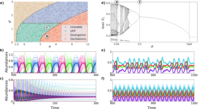
Figure 2: Stabilization of macroscopic dynamics when adding disorder. a) The phase diagram for the 3-group RPS system comprises three main regions: unique fixed point (green), low-dimensional macroscopic oscillations (red) and high-dimensional microscopic chaos (blue), as well as a divergent region (yellow) where the LV model is meaningless [2]. Solid lines denote analytically predicted transitions from and to equilibrium, while dotted lines denote extrapolations in nonequilibrium regimes. In the area between $\kappa=3$ and $\kappa\approx 7$, disorder first stabilizes the macroscopic modes to a fixed point. b) and c) Two examples of dynamics for the 3-group system along the $\kappa=4$ line, at $\sigma=0.3$ and $\sigma=1$. The macroscopic dynamics (average abundance per group) are plotted as thick lines. A subset of species trajectories is shown as thin lines. While species within each group initially follow the same trend, disorder progressively leads to a mismatch in their trajectories and finally stabilization. d) Bifurcation diagram for the 4-group system showing the local maxima of the abundance of the first group as a function of $\sigma$. Starting from low-dimensional chaotic dynamics at $\sigma=0$, the system undergoes a series of period-halving bifurcations leading to simpler oscillations, until a Hopf bifurcation to a fixed point. e) and f) Examples of dynamics for the 4-group system at $\sigma=0.04$ and $\sigma=0.2$, with chaotic and cyclic dynamics respectively.

We consider interaction structures $\mu_{ij}$ that induce nonequilibrium dynamics for the macroscopic variables. Two examples will be used for illustration purposes, both with a block structure (i.e. the macroscopic observables are the total abundances of groups of equivalent species): a simple Rock-Paper-Scissors (RPS) matrix with within-group coefficient $u$ and between-group coefficient $\kappa$ (Fig. 1a), leading to cyclic behavior (Fig. 1b), and a 4-group matrix [6] (coefficients in Appendix B) that produces a low-dimensional chaotic trajectory (Fig. 1c,d).

We first show numerically in Fig. 2 that the addition of microscopic disorder can stabilize these low-dimensional macroscopic dynamics. In the RPS example, in the absence of disorder $\sigma=0$, species within groups are identical in abundance and dynamics, and the trajectories are periodic for $\kappa>2(u+1)$; otherwise they reach a symmetric fixed point where all groups have identical abundance. Increasing $\sigma$ leads to different dynamical regimes, and we give the phase diagram in Fig. 2a. First, the intrinsic timescales of species within each group become increasingly mismatched (Fig. 2b) due to abundance heterogeneity. While coupling between groups forces the dynamics to stay synchronized, species trajectories are now spread. For moderate $\kappa$, increasing disorder $\sigma$ finally leads to the stabilization of a fixed point that recovers the group-level symmetric solution despite abundances withing groups being spread due to randomness (Fig. 2c). In the case of the 4-group structure, Fig 2d shows that increasing $\sigma$ rewinds the whole Feigenbaum cascade, i.e. a series of period-halving bifurcations leads back from chaos (Fig. 2 e) to limit cycles (Fig. 2 f) until a final Hopf bifurcation to a fixed point. This hints at a general ability of microscopic disorder to simplify macroscopic dynamics, both by stabilizing fixed points and by inducing bifurcations between out-of-equilibrium regimes.

As we further increase $\sigma$, we also see that disordered interactions destabilize the microscopic variables. We observe a phase transition, now well understood in Random LV (when $\mu_{ij}=\mu$) [7, 8], to a regime with many marginal or unstable fixed points, usually characterized by high-dimensional chaotic dynamics [9, 3] (barring special symmetries [10, 11, 12]). Similar transitions have been studied in other disordered systems such as random neural networks [13]. Fig. 2a at high $\sigma$ and $\kappa$ further shows a direct transition from macroscopic cycles to high-dimensional chaos, whose characterization is beyond the scope of this letter. In any case, we show in Supplementary Materials that the coarse-grained observables are only weakly impacted by this chaotic regime, and thus, disorder is overall more stabilizing than destabilizing at the macroscopic scale.

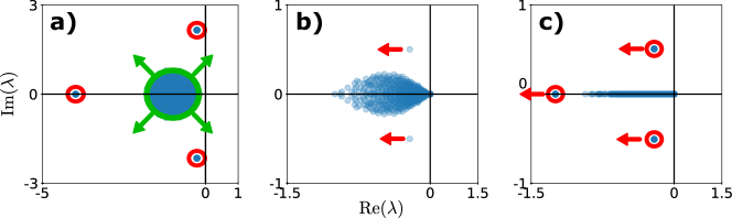
Figure 3: Spectral contributions of macroscopic structure and microscopic disorder. The spectra of a) the interaction matrix $A$, b) the Jacobian and c) the pseudo-Jacobian (defined in eq. (8)) comprise a bulk stemming from disorder (outlined in green) and outliers stemming from structure (outlined in red). As $\sigma$ increases, the bulk expands while the outliers of $A$ remain unchanged, but the outliers of the Jacobian and the pseudo-Jacobian are pushed to the left (arrows).

Decoupling of low-dimensional and high-dimensional dynamics: We now analyze why microscopic interaction disorder appears here to generally stabilize low-dimensional macroscopic dynamics. Matrices of the form given in eq. (7) have previously been studied from the perspective of Random Matrix Theory. It is known [14] that their spectra features outliers at the same locations as the eigenvalues of $\mu_{ij}$ and that, conversely, these outliers do not influence the bulk stemming from $\xi_{ij}$ (see Fig. 3a). This spectral simplicity has its counterpart in the behavior of the ecological model.

A full analysis using Dynamical Mean Field Theory (well-established for this class of dynamical models [9], details in Appendix C), shows that structure and disorder contribute separate terms to the dynamics. Disorder alone drives the transition to high-dimensional chaos noted above, with no impact from structure, and the location of this instability can be deduced only from the interaction matrix $A$, without computing the Jacobian of the dynamics. By contrast, the transitions associated with the macroscopic modes appear in the Jacobian and not in $A$. Our analysis (see Appendix D) shows that these transitions can be located by computing the mean over disorder of the deviations from equilibrium

$$\frac{\mathrm{d}}{\mathrm{d}t}\langle\vec{\delta x}(t)\rangle=\mathcal{J}\cdot\langle\vec{\delta x}(t)\rangle,$$

with the following ’pseudo-Jacobian’ matrix

$$\mathcal{J}_{ij}^{\star}=-r_{i}x_{i}^{\star}\left(\delta_{ij}-\frac{1}{S}\mu_{ij}\right),$$ (8)

restricted to non-extinct species, where $x_{i}^{\star}>0$ are their equilibrium abundances. Crucially, even though $\mathcal{J}$ resembles the Jacobian of the LV system, it no longer explicitly contains the disordered part of the interactions. Hence, every result going forward is equivalent to ignoring the disordered components $\xi_{ij}$ except for their impact on the row coefficients in $\mathcal{J}$, i.e. the dynamical rates controlled by the equilibrium abundances $x_{i}^{\star}$.

This pseudo-Jacobian $\mathcal{J}$ is an instance of the form eq. (4) studied earlier, having replaced $r_{i}$ by $r_{i}x_{i}^{\star}$. We hereafter consider $r_{i}=1$ and focus on the effect of increasing interaction disorder $\sigma$: it causes a random spread in the abundances of surviving species $x_{i}^{\star}$, thus a mismatch between their dynamical time scales that impacts the eigenvalues of the pseudo-Jacobian. These findings are summarized in Fig. 4, where we plot how eigenvalues of the Jacobian of the 3-group RPS model change with increasing $\sigma$, as well as the flow predicted by eq. (5) for a distribution of $r_{i}$ equal to the distribution of abundances $x_{i}^{\star}$ obtained from DMFT.

Thus the equivalence between time-scales in eq. (4) and abundances in the Lotka-Volterra model provides an analytical argument for the stabilization of eq. (8) as $\sigma$ increases. Strictly speaking, it holds only when the $x_{i}^{\star}$ are identically distributed, owing to the assumptions made in eq. (5). This is true for all matrices $\mu$ having $(1,\dots,1)$ as an eigenvector (as the 3-group RPS case), where the fixed point and thus the flow in Fig. 4 are independent of the structure of $\mu$. More generally, we expect the same qualitative behavior as long as microscopic time scale distributions are sufficiently similar across species. However, numerical simulations suggest that this is a more general property that transcends the existence of particular symmetries, as seen in our 4-group example.

We finally note that the spread of equilibrium species abundances $\vec{x}^{\star}$ induced by disorder could also stabilize the group dynamics through a different mechanism: changing the coefficients in $\mu$. In the general form eq. (4), this could happen through nonlinearities in how microscopic dynamics $\vec{G}$ depend on coarse-grained variables $\vec{f}$, and $\vec{f}$ on $\vec{x}$. In our simpler setting, with the LV model and $\vec{f}$ being linear combinations of abundances, the only such nonlinearity stems from species extinctions, $x_{i}^{\star}=0$, since surviving species then experience fewer interactions and different parameters on average [15, 16]. We observe in Supplementary Materials that this effect is present, yet intervenes only at larger values of $\sigma$, and is therefore not responsible for stabilization here.

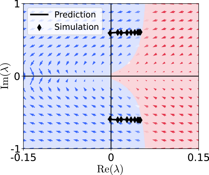
Figure 4: Increasing abundance and time scale heterogeneity stabilizes the outlier eigenvalues. Diamonds are leading eigenvalues of the true Jacobian $J$ in simulations of the 3-group LV system with increasing disorder, for ten values of $\sigma$ between 0 and 0.5, and fixed parameters $u=0.5$ and $\kappa=3.5$. The thick lines are the analytical prediction from the evolution equation of the pseudo-Jacobian $\mathcal{J}$, eq. (5), with fixed-point abundances $x^{\star}$ instead of rates $r$, using the distribution $\rho(x^{\star})$ predicted by DMFT. The background arrows show the vector field of eq. (5) for the abundance distribution $\rho_{0}(x^{\star})=\delta(x^{\star}-1/(1+u+\kappa))$, which is the equilibrium solution in the absence of disorder. Note that, as the abundance distribution changes with increasing disorder, so does the r.h.s of eq. (5); hence the vector field is a snapshot for a particular value of $\tau$, in this case $\tau=0$. Background colors indicate regions for which an eigenvalue starting within will (blue) and will not (red) reach stability as $\sigma$ reaches 0.5.

Conclusions: In a system with out-of-equilibrium dynamics originating at the macroscopic scale, the addition of microscopic complexity can have a stabilizing effect – in particular when it creates a spread in the characteristic time scales of microscopic trajectories, as in eq. (8). This spread can be a direct consequence of heterogeneous rate parameters, or, as we found, an indirect consequence of disorder in interactions (nonlinearity is then required, as this effect arises in how the Jacobian matrix differs from the bare interaction matrix).

This stabilization mechanism qualitatively recalls a phenomenon found in systems of coupled oscillators, where a diversity in intrinsic time scales can induce the emergence of a stable equilibrium [17, 18, 19, 20]. In both cases, a mismatch of intrinsic timescales between coupled variables seems to be key in damping the dynamics. Yet, our work puts more emphasis on the tension between levels of description: here, an instability is induced by macro-scale interactions, and damped by micro-scale disorder. This holds even when the micro-scale consequences of adding disorder tend to be a loss of stability (i.e. the well-studied destabilizing effect of complexity [21] and transition to high-dimensional chaos [22, 2, 8]).

The ecological systems studied here could provide archetypal examples of this phenomenon (as perhaps other systems with multiplicative growth properties, e.g. in economics [23]). Recently, high-throughput methods for acquiring data on ecological and especially microbial communities have revealed ubiquitous fluctuations and heterogeneity at species and sub-species levels [24, 25]. Yet, more macroscopic descriptions, based on large taxonomic groups or ecological functions, are markedly stable across systems and over time [26, 27]. It remains to be seen whether this macroscopic stability has other causes (e.g. physico-chemical constraints or simple aggregation effects) or truly results from species-level disorder damping ecosystem-level dynamics, and why this stabilizing mechanism might not already act at species level from sub-species disorder.

While our mathematical analysis only captures local transitions to and from a fixed point, the qualitative intuition of the stabilizing mechanism seems to hold more generally: for instance, the 4-group system in Fig. 2 switches from chaos to cycles before the fixed point is stabilized. Understanding these transitions analytically provides a theoretical challenge that we believe is worth addressing in the future.

Appendix A A. Effect of time scale disorder on eigenvalues

To study the spectrum of $J$ (defined in eq. (4)), we may take advantage of the low rank of $\mu$ to reduce the problem to that of inverting a small matrix. In particular, if $n=\mathrm{rank}(\mu)$, there exist $S\times n$ matrices $U,V$ such that $\mu=UV^{T}$. Using Woodbury’s matrix identity, we then find that $z\in\mathbb{C}$ is an outlier eigenvalue of $J$ iff

$$\mathrm{det}\left(\mathbb{I}_{n\times n}-V^{T}\cdot\mathrm{diag}\left\langle\frac{r}{z+r}\right\rangle\cdot U\right)=0,$$ (9)

where the average is taken w.r.t. the distribution of time scales $r_{i}$.

In order to understand the effect of time scale spread, we will tune it up in eq. (9) in a continuous way. Starting from constant rates, e.g. $r_{i}(\tau=0)=1$, we let $x_{i}^{\star}(\tau+\mathrm{d}\tau)=x_{i}^{\star}(\tau)+\sqrt{x_{i}(\tau)\mathrm{d}\tau}\eta_{i}$ where $\eta_{i}$ is a standard Gaussian variable. This defines a diffusion process in ’rate space’ that causes the outliers of $J$ to undergo a deterministic process. Linearizing eq. (9) we find that

$$\frac{\mathrm{d}z}{\mathrm{d}\tau}=-z\frac{\bra{u_{z}}\mathrm{diag}\left(\left\langle\frac{r}{(z+r)^{3}}\right\rangle\right)\ket{v_{z}}}{\bra{u_{z}}\mathrm{diag}\left(\left\langle\frac{r}{(z+r)^{2}}\right\rangle\right)\ket{v_{z}}},$$ (10)

where we define $u_{z},v_{z}$ such that $V^{T}\mathrm{diag}\left(\frac{r}{z+r}\right)U\ket{v_{z}}=\ket{v_{z}}$ and $\bra{u_{z}}V^{T}\mathrm{diag}\left(\frac{r}{z+r}\right)U=\bra{u_{z}}$, and we have normalized $\braket{u_{z}}{v_{z}}=1$. Leveraging the fact that all the $r_{i}(\tau)$ have the same distribution (a fact that stems from the equality in initial conditions), eq. (10) can be rewritten in a simpler form

$$\frac{\mathrm{d}z}{\mathrm{d}\tau}=-z\left\langle\frac{r}{(z+r)^{3}}\right\rangle\left\langle\frac{r}{(z+r)^{2}}\right\rangle^{-1},$$

which is exactly eq. (5) from the main text.

Appendix B B. Low-dimensional chaos

We follow [6] in constructing the following 4-species Lotka-Volterra system that exhibits low-dimensional chaos

$$\vec{r}=\begin{pmatrix}1\\ 0.72\\ 1.53\\ 1.27\end{pmatrix},\qquad A=\begin{pmatrix}1&1.09&1.52&0\\ 0&1&0.44&1.36\\ 2.33&0&1&0.47\\ 1.21&0.51&0.35&1\end{pmatrix}$$ (11)

Here the time scale heterogeneity (in $\vec{r}$) is required to destabilize the fixed point and induce chaotic dynamics, illustrating the fact that the stabilizing effect of such heterogeneity is a high-dimensional effect and not generic for a few-variable system.

Appendix C C. Dynamical Mean-Field Theory for gLV

Let us again denote $\mu=UV^{T}$ where $U,V$ are $S\times n$ matrices of coefficients $u_{i}^{(\alpha)},v_{i}^{(\alpha)}$. Such matrices can be obtained from the Singular Value Decomposition (SVD) of $\mu$. We use the well-established framework of Dynamical Mean-Field Theory [22, 28, 29] to reduce the high-dimensional dynamics of eq. (2) to an effective one-dimensional stochastic differential equation,

$$\frac{\mathrm{d}x_{i}}{\mathrm{d}t}=r_{i}x_{i}\left(1-x_{i}+\sum_{\alpha}u_{i}^{(\alpha)}f_{\alpha}(t)+\sigma\zeta_{i}(t)\right),$$ (12)

where $\zeta_{i}$ are Gaussian processes with zero mean and correlation $\langle\zeta_{i}(t)\zeta_{j}(s)\rangle=\delta_{ij}\langle x(t)x(s)\rangle$ and $f_{\alpha}(t)$ are mean-field variables (henceforth called functions) independent of the realization of randomness, given by $f_{\alpha}(t)=S^{-1}\sum_{i}v^{(\alpha)}_{i}\langle x_{i}(t)\rangle$. Here, brackets indicate averages w.r.t. the stochastic processes $\zeta_{i}$.

This effective process may undergo different dynamical regimes depending on the model parameters. In particular, the system may reach a fixed where all time-dependent quantities converge, $x_{i}(t)\rightarrow x_{i}^{\star},\zeta_{i}(t)\rightarrow\zeta_{i}^{\star},f_{\alpha}(t)\rightarrow f_{\alpha}^{\star}$. The fixed-point abundances are then given by

$$x_{i}^{\star}=\max\left(0,1+\sum_{\alpha}u_{i}^{(\alpha)}f_{\alpha}^{\star}+\sigma\zeta_{i}^{\star}\right),$$

and therefore follow truncated Gaussian distributions. This equation, along with the self consistent relations $\langle(\zeta_{i}^{\star})^{2}\rangle=S^{-1}\sum_{j}\langle(x_{j}^{\star})^{2}\rangle$ and $f_{\alpha}^{\star}=S^{-1}\sum_{i}u_{i}^{(\alpha)}\langle x_{i}^{\star}\rangle$, can be used to find the values of $f_{\alpha}^{\star}$ and the distribution of $\zeta_{i}^{\star}$, which are enough to characterize the equilibrium. In turn, other quantities of interest, such as the fraction of surviving species $\phi^{\star}$, can be obtained from them.

For our purposes, the most important aspect of such relations is that, as $\sigma$ is increased from $0$, the spread of each Gaussian increases, leading to a spread in the Species Abundance Distribution.

Appendix D D. Stability

Stability is analysed by linearizing the effective equation eq. (12) and adding a small perturbation $\delta x_{i}(t)=x_{i}(t)-x_{i}^{\star}$. This is equivalent to calculating the Jacobian of the system at the given fixed point. We obtain

$$\begin{split}\frac{\mathrm{d}}{\mathrm{d}t}\delta x_{i}&=\delta x_{i}\left(1-x_{i}+\sum_{\alpha}u_{i}^{(\alpha)}f_{\alpha}^{\star}+\sigma\zeta_{i}^{\star}\right)\\ &+x_{i}^{\star}\left(-\delta x_{i}+\sum_{\kappa}u_{i}^{(\alpha)}\delta f_{\alpha}+\sigma\delta\zeta_{i}\right),\end{split}$$

where stars indicate fixed point quantities. The quantities $\delta f_{\alpha}$ and $\delta\zeta_{i}$ are respectively perturbations to the functions and the DMFT noise, induced by the perturbations in the abundances. They are characterized by $\langle\delta f_{\alpha}(t)\rangle=S^{-1}\sum_{i}u_{i}^{(\alpha)}\langle\delta x_{i}(t)\rangle$ and $\langle\delta\zeta_{i}(t)\delta\zeta_{j}(s)\rangle)=\delta_{ij}\langle\delta x_{i}(t)\delta x_{j}(s)\rangle$.

The first term in the r.h.s is zero for extant species and negative for extinct species. Hence it cannot cause an instability. Hence we will focus on the second term. Even though only extant species have it non-zero, we will consider it for all species, for mathematical convenience.

Because the equation is linear and $\delta\zeta_{i}$ is a Gaussian process, $\delta x_{i}$ is also a Gaussian process. We may therefore analyse it through its mean and auto-correlation, and characterize stability by requiring that both quantities tend to zero at infinity. Starting with the variance, an analysis similar to [28] gives the stability condition

$$1>\phi^{\star}\sigma^{2},$$

where $\phi^{\star}$ is the fraction for surviving species at equilibrium. This characterizes the collective transition to instability well-studied in previous works. Here, we are mainly concerned with structure-driven transitions, which will be signalled by the mean, for which we obtain the system of ODEs

$$\frac{\mathrm{d}}{\mathrm{d}t}\langle\vec{\delta x}(t)\rangle=\mathcal{J}\cdot\langle\vec{\delta x}(t)\rangle,$$

where the matrix $\mathcal{J}$ is given by $\mathcal{J}_{ij}=-r_{i}x_{i}^{\star}\left(\delta_{ij}-\mu_{ij}/S\right)$. This ’pseudo-Jacobian’ is akin to the Jacobian of the Lotka-Volterra system without dirorder except for the fact that the abundances $x_{i}^{\star}$ are influenced by randomness. The spectrum of $\mathcal{J}$ is composed of a bulk stemming from the diagonal component and a few outliers stemming from the non-zero eigenvalues of $\mu$.

Supplementary Material

Appendix A Ecological context

Ecosystems are complex systems composed of a large number of units whose properties are distributed, and that are in interaction with one another. As many biological details are unknown, ecosystem models often abstract away microscopic complexity and describe the low-dimensional dynamics of energy and material fluxes [1] or of broad classes of species (e.g. phytoplankton and zooplankton). Even when heterogeneity between species is taken into account, it typically ignores intraspecific strain diversity [30]. More generally, when comparing abstract models with observations, some degree of coarse-graining is inevitable, and theoretically justified when the macroscopic degrees of freedom reflect the properties of the microscopic ones.
If heterogeneity can be ignored in physical systems whose microscopic dynamics and parameters are largely homogeneous, the meaning of coarse-grained descriptions can be questioned for complex systems with strong microscopic variation. This is the case of microbial ecosystems, where high-throughput molecular methods revealed that stable patterns of community-level descriptors may overshadow extensive variability at the species and sub-species level [26, 27, 25].

Ecology has long investigated the relationship between complexity and stability. The traditional view holds that volatile population dynamics are more likely in few-species systems (e.g. boreal forests, with boom and bust cycles of lynxes and hares) than in many-species ones (e.g. tropical forests, where perturbations may diffuse incoherently across many interaction pathways) [31]. Yet, a seemingly opposite claim inspired by Random Matrix Theory has come to prominence: Robert May famously noted that no generic mathematical result supports the idea of stabilizing complexity – on the contrary, a simple model of linearized dynamics with random coefficients predicts that a fixed point goes from stable to unstable when increasing the number and heterogeneity (variance) of interactions [21], as recently supported by microbial experiments [3].

However, none of these works directly investigate the central question here: whether complexity understood as disorder at a microscopic level might stabilize a model that exhibits out-of-equilibrium dynamics at a macroscopic level. Our key mechanism is through a loss of coherence of microscopic dynamics when their time scales become heterogeneous.

We also noted a distinct mechanism of stabilization via a reduction of effective interactions. This mechanism is not the one driving the stabilization of the oscillatory modes considered here, but can remove macroscopic instabilities associated with real positive eigenvalues, such as bistability [32].

This reduction of effective interactions can arise either from inter-group interactions being weaker, or from within-group and within-species interactions being stronger. The latter can happen through feedbacks: as $\sigma$ increases, when interactions are not i.i.d., the effective self-interaction of a species may increase, see the section “Symmetry of interactions” below.

Another possibility is through nonlinearities. In our LV model, the only relevant nonlinearity is species extinctions, see the next section. Yet other recent studies discuss another nonlinearity-based mechanism, when single-species dynamics and interaction terms have different nonlinearities, e.g. with the so-called theta-logistic model $r(x)=(1-x^{\theta})/\theta$ [33, 34]. If $\theta<1$, increasing system size (number of species) can stabilize by pushing the average abundance towards lower values where the single-species potential is more confining – the negative diagonal elements of the Jacobian matrix become larger compared to the off-diagonal elements. We note however that in these works, stabilization happens when increasing the number of species, not when increasing the heterogeneity of their interactions (which typically remains destabilizing). Confusions may thus arise since May’s notion of “complexity” combined species number and variance of their interaction strengths [21], which have opposite effects in these models, leading to divergent answers as to whether complexity stabilizes or destabilizes the system.

Appendix B Stabilization by species extinctions

We show in Figure S1 how an increase in interaction heterogeneity $\sigma$ leads to a stabilization of the outlier eigenvalue pair associated with the unstable mode in the rock-paper-scissors structure. Figures S2 and S3 illustrate in more detail the dynamical trajectories of species abundances and the spectrum of the Jacobian and reduced interaction matrix for four different values of $\sigma$.

These figures show that stabilization through desynchronization, which can be seen in the Jacobian matrix, happens ahead of stabilization through extinctions, which can be seen in the reduced interaction matrix (restricted to non-extinct species).

Figure S1: Displacement of the outlier eigenvalue pair in Lotka-Volterra simulations when increasing disorder $\sigma$ over $[0.4,2.2]$ in increments of 0.1. Positive eigenvalues are shown in red. (a) and (b) show the good approximation of the outlier eigenvalues of the real Jacobian matrix (a) with those of the pseudo-Jacobian eq. (8) where disordered interactions have been removed (b). (c) shows that species extinctions can eventually stabilize this mode in the reduced interaction matrix $A^{\star}$, but only at higher values of $\sigma$ (10 steps are needed instead of 4). (d) shows that the outliers of the full interaction matrix $A$ are only weakly affected by the addition of increasing disorder.

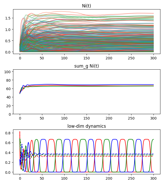
(a) (b)
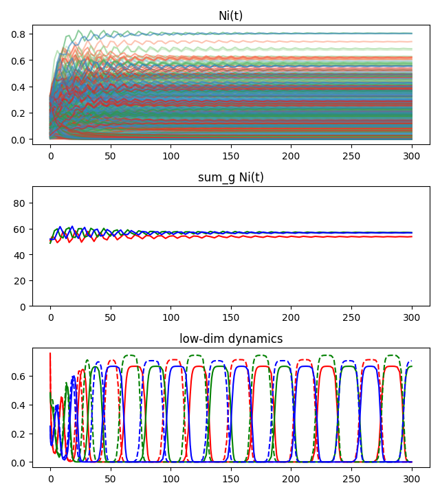
(c) (d)

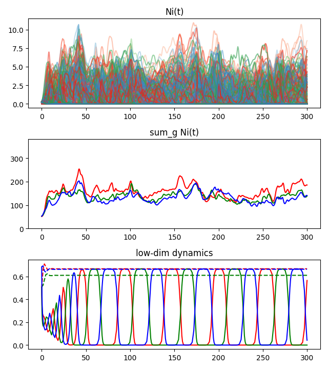
Figure S2: Species abundance trajectories for $\sigma\in[0.4,0.8,1.4,2.2]$ (a,b,c,d). From top to bottom: trajectories of individual species abundances (colored by group), sum of abundances within a group, and trajectories for the corresponding 3-species system (solid line: averaging parameters over all species within a group, dashed line: averaging parameters over surviving species only)

(a)
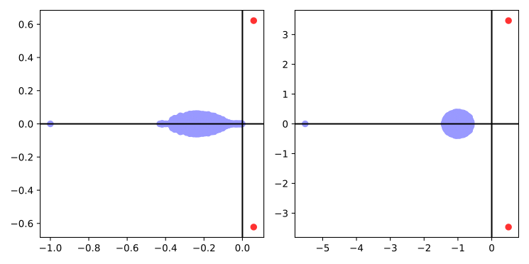
(b)
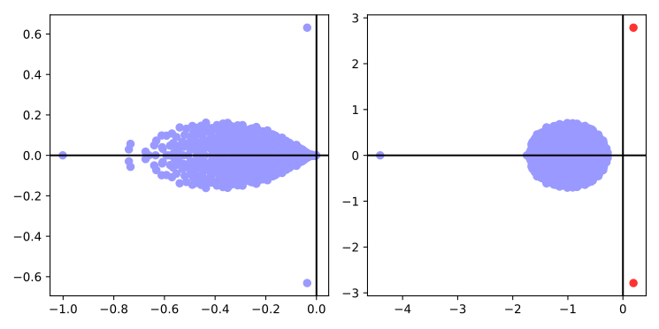
(c)
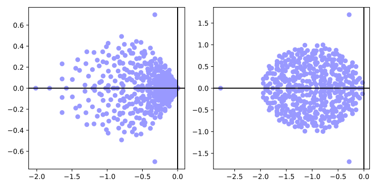
(d)

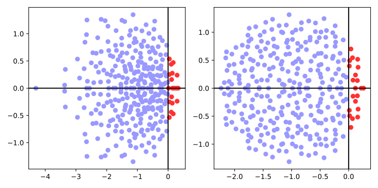
Figure S3: Spectra (left: Jacobian matrix, right: matrix $A^{\star}$ restricted to surviving species) for $\sigma\in[0.4,0.8,1.4,2.2]$ (a,b,c,d). Eigenvalues with positive real part are shown in red.

Appendix C Symmetry of interactions

Previous works on the random Lotka-Volterra model have studied the influence of correlations between transpose terms in the interaction matrix. It has been shown that the parameter $\gamma=\langle\xi_{ij}\xi_{ji}\rangle$ changes the shape of the spectral bulk of $A$, hence impacting the location of the collective transition to chaotic dynamics [28, 2]. Once the structural matrix $\mu$ is added, $\gamma$ turns out to also affect the location of the outliers, hence the location of the outliers of the Jacobian and ultimately the stability of the system.
To generalize the calculations in Appendices C and D to take $\gamma\neq 0$ into account (see, e.g. [28]), the linear response functions of the system need to be introduced,

$$G_{i}(t,s)=\left\langle\frac{\delta x_{i}(t)}{\delta r_{i}(s)}\right\rangle\text{ and }G(t,s)=S^{-1}\sum_{i}{G_{i}(t,s)}.$$

Close to the fixed point, there quantities are assumed to be time-translation-invariant (TTI) so that $G_{i}(t,s)=G_{i}(t-s)$ and we may introduce their Fourier transforms which are shown to equal

$$G_{i}(\omega)=\frac{1}{2\gamma\sigma^{2}}\left(1+\frac{i\omega}{x_{i}^{\star}}\pm\sqrt{\left(1+\frac{i\omega}{x_{i}^{\star}}\right)^{2}-4\gamma\sigma^{2}\phi}\right),$$

where the branch is taken so that a finite limit exists for $\gamma\rightarrow 0$. Linearizing the dynamical equation and taking its average as in Appendix D, and finally taking Fourier transforms yields the criticality condition

$$\exists\omega\in\mathbb{R},\mathrm{det}\Big{[}i\omega+x_{i}^{\star}\left(\left(1-\gamma\sigma^{2}G(\omega)\right)\delta_{ij}-\mu_{ij}\right)\Big{]}=0.$$ (S1)

The stability of the system can then be assessed by solving this equation for $\omega\in\mathbb{C}$. If $\mathrm{Re}(i\omega)>0$, the fixed point is unstable, it is stable otherwise. For $\gamma=0$, eq. (S1) defines $i\omega$ as an eigenvalue of the pseudo-Jacobian $\mathcal{J}$, and the criterion from the main text is recovered. Using Woodbury’s identity, and decomposing $\mu=UV^{T}$ with $U$ of shape $S\times n$ this is equivalent to solving the low-dimensional problem

$$\mathrm{det}\left[\mathbb{I}_{n\times n}-V^{T}\cdot\mathrm{diag}\left\langle\frac{x^{\star}}{i\omega+x^{\star}\left(1-\gamma\sigma^{2}G(\omega)\right)}\right\rangle\cdot U\right]=0$$

Fig. S4 gives the phase diagram of the RPS system in the $(\gamma,\sigma)$ plane for fixed parameters $u=0.5$ and $\kappa=4$. With regards to macroscopic oscillations, skew-symmetric disorder is seen to be less stabilizing that symmetric disorder (solid line). This runs counter to the rule for the collective transition (dashed line), where symmetric interactions are less stable due to the emergence of positive feedback loops.

Figure S4: Phase diagram of the RPS system in the presence of transpose correlations ($u=0.5,\kappa=4$). The transition from macroscopic oscillations to stability is favored by symmetric interactions ($\gamma=1$), although symmetric interactions also favor the collective transition to chaotic fluctuations (dashed line), which happens at $\sigma=\sqrt{2}/(1+\gamma)$. Lines and background colors are theoretical predictions, while dots are simulations with $S=3000$ species.

Appendix D Optimality of disorder

We can complement the argument in the main text with a converse argument by asking: given an abundance configuration $\vec{x}^{\star}$, what is the angle between the infinitesimal modification $\delta\vec{x}^{\star}$ that most increases the stability of a given eigenvalue and the modification that most increases the variance? This is done by taking the dot product

$$\delta\vec{x}^{\star}=-\vec{\nabla}\mathrm{Re}(\lambda)\cdot\vec{x}^{\star}+S\left\langle\vec{\nabla}\mathrm{Re}(\lambda)\right\rangle\langle x^{\star}_{i}\rangle,$$

between the gradient of a given eigenvalue and the gradient of the variance of abundances, both projected so as to eliminate the effect of total abundance. Taking the three-group interaction matrix of Fig. 1 as an example, Fig. S5 shows that the angle thus obtained is much smaller than $90^{\circ}$ for most of the complex plane, with faster-oscillating modes being again the ones for which increasing the variance is closest to optimal stabilization.

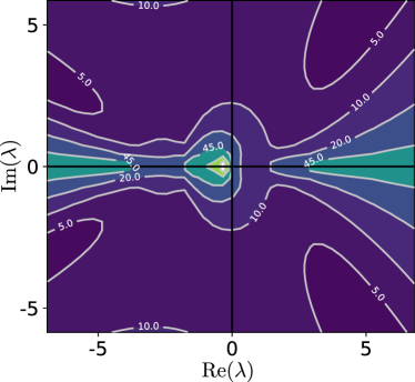
Figure S5: Increasing heterogeneity is close to optimal for stabilizing the RPS system. We calculate the eigenvalues $\lambda$ of $\mathcal{J}$ for many values of $u,\kappa$ and some equilibrium configuration $x^{\star}$. We calculate the change in $x^{\star}$ that maximizes the displacement of $\lambda$ towards the left (while keeping $\langle x^{\star}\rangle$ fixed, to avoid the spurious effect of reducing the overall abundance), and plot the angle between that direction and the direction that most increases the variance of $x^{\star}$.

Unfortunately, while this property appears to hold in our chosen examples, we have no analytical argument for its generality (in particular, results may depend on eigenvectors and not only on the eigenvalues themselves as in eq. (5)), and thus retain it here only as a promising direction for future investigations.