Gill and Massar type bound for estimation of $SU(2)$ channel

Abstract

In the estimation for a parametric family of quantum state on a Hilbert space $\mathcal{H}$, the Gill and Massar bound is known as a lower bound of weighted traces of covariances of unbiased estimators. The Gill and Massar bound is derived by considering the convexity of the set of classical Fisher information matrices, and the bound is locally achievable by using randomized strategies when $\mathcal{H}=\mathbb{C}^{2}$. In this paper, we show that estimation for a parametric $SU(2)$ unitary channel model has a similar convex structure as qubit state model, and a Gill and Massar type lower bound of weighted traces of covariances of unbiased estimators can be derived for any weight matrix. We show that the Gill and Massar type lower bound is achievable by using randomized strategies when certain conditions are satisfied. To derive a convex structure of the set of classical Fisher information matrices, we introduce a Fisher information matrix $J^{(U)}$ for a $SU(2)$ unitary channel model, and we show a upper bound of inverse $J^{(U)}$ weighted trace of classical Fisher information matrix. The optimal randomized strategy we construct in this paper does not require ancilla systems in many cases.

1 Introduction

Quantum state estimation and quantum channel estimation are important topics in quantum information processing. When dealing with multi-parameter models, the estimation problem is complicated due to the non-commutativity in quantum mechanics[1, 2, 3, 4]. This paper deals with the $SU(2)$ unitary channel estimation problem based on quantum state estimation theory, so let us begin with an introduction to the state estimation.

Let $\mathcal{S}(\mathcal{H})$ be a set of density operators on a Hilbert space $\mathcal{H}$. In quantum state estimation theory of a parametric family of density operators $\left\{\rho_{\theta}\in\mathcal{S}(\mathcal{H})\mid\,\theta\in\Theta\subset\mathbb{R}^{d}\right\}$, an estimator is a pair $(M,\hat{\theta})$ of a POVM $M$ taking values in a finite set $\mathcal{X}$ and a map $\hat{\theta}:\mathcal{X}\mapsto\Theta$. An estimator $(M,\hat{\theta})$ is called unbiased if

$$E_{\theta}[M,\hat{\theta}]=\sum_{x\in\mathcal{X}}\hat{\theta}(x){\rm Tr}\,\rho_{\theta}M_{x}=\theta$$ (1)

is satisfied for all $\theta\in\Theta$. An estimator $(M,\hat{\theta})$ is called locally unbiased [5] at a fixed point $\theta_{0}\in\Theta$ if the condition (1) is satisfied around $\theta_{0}$ up to the first order of the Taylor expansion, i.e.,

$$\sum_{x\in\mathcal{X}}\hat{\theta}^{i}(x){\rm Tr}\,\rho_{\theta_{0}}M_{x} =\theta_{0}^{i}\qquad(i=1,\dots,d),$$

$$\sum_{x\in\mathcal{X}}\hat{\theta}^{i}(x){\rm Tr}\,\partial_{j}\rho_{\theta_{0}}M_{x} =\delta_{j}^{i}\qquad(i,j=1,\dots,d),$$

where $\partial_{j}\rho_{\theta_{0}}=\left.\frac{\partial}{\partial\theta^{j}}\rho_{\theta}\right|_{\theta=\theta_{0}}$. To find optimal estimator, lower bounds of the weighted trace of the covariance matrix ${\rm Tr}\,WV_{\theta_{0}}[M,\hat{\theta}]$ for a locally unbiased estimator $(M,\hat{\theta})$ was investigated, where $W$ is a $d\times d$ positive real matrix and $V[M,\hat{\theta}]$ is the covariance matrices. Because of the classical Cramér-Rao inequality $V_{\theta_{0}}[M,\hat{\theta}]\geq J_{\theta_{0}}^{(C,M)^{-1}}$ with the classical Fisher information matrix

$$J_{\theta_{0},ij}^{(C,M)}=\sum_{x\in\mathcal{X}}\frac{\left({\rm Tr}\,\partial_{i}\rho_{\theta_{0}}M_{x}\right)\left({\rm Tr}\,\partial_{j}\rho_{\theta_{0}}M_{x}\right)}{{\rm Tr}\,\rho_{\theta_{0}}M_{x}},$$

and its sharpness, $\inf_{(M,\hat{\theta})}{\rm Tr}\,WV_{\theta_{0}}[M,\hat{\theta}]$ is identical to $\inf_{M}{\rm Tr}\,WJ_{\theta_{0}}^{(C,M)^{-1}}$.

When $\dim\mathcal{H}$=2, it is known that ${\rm Tr}\,WV[M,\hat{\theta}]$ satisfies the following inequality:

$${\rm Tr}\,WV_{\theta_{0}}[M,\hat{\theta}]\geq c_{\theta_{0},W}^{(GM)}$$

with the Gill and Massar bound

$$c_{\theta_{0},W}^{(GM)}:=\left({\rm Tr}\,\sqrt{J_{\theta_{0}}^{(S)^{-1/2}}WJ_{\theta_{0}}^{(S)^{-1/2}}}\right)^{2},$$ (2)

where $J_{\theta_{0}}^{(S)}$ is the symmetric logarithmic derivative (SLD) Fisher information matrix [6, 7] (see also [8]). The lower bound $c_{\theta_{0},W}^{(GM)}$ is achievable by using a randomized strategy of $d$ projective measurements for $d=2,3$. The bound $c_{\theta_{0},W}^{(GM)}$ can be derived by using the convex structure of the set $\mathcal{F}_{\theta_{0}}:=\left\{J_{\theta_{0}}^{(C,M)}\mid M\text{ is a POVM}\right\}$ of classical Fisher information matrices. In the estimation of a qubit state model $\left\{\rho_{\theta}\in\mathcal{S}(\mathbb{C}^{2})\mid\theta\in\Theta\subset\mathbb{R}^{3}\right\}$, the set $\mathcal{F}_{\theta_{0}}$ of classical Fisher information matrices satisfies

$$\mathcal{F}_{\theta_{0}}=\left\{F\mid F\text{ is a $d\times d$ real positive matrix such that }{\rm Tr}\,J^{(S)^{-1}}F\leq 1\right\}.$$

Thus finding the minimum of weighted trace of covariance matrices for a weight $W$ is reduced to the convex optimization problem to find

$$\min_{F\in\mathcal{F}_{\theta_{0}}}{\rm Tr}\,WF^{-1}(=c_{\theta_{0},W}^{(GM)}),$$

and the minimum is achieved by a randomized strategy. In this paper, we show that the estimation of $SU(2)^{\otimes n}$ channel has a similar structure and a similar bound can be derived.

Let $\left\{U_{\theta}\mid\,\theta\in\Theta\subset\mathbb{R}^{d}\right\}$ be a parametric family of $SU(2)$ unitary matrices on a Hilbert space $\mathcal{H}=\mathbb{C}^{2}$ with $d=1,2,3$, and let us consider a corresponding parametric family of unitary channels

$$\left\{\Gamma_{\theta}:\mathcal{B}(\mathbb{C}^{2})\to\mathcal{B}(\mathbb{C}^{2}),\,\rho\mapsto U_{\theta}\rho U_{\theta}^{*}\mid\,\theta\in\Theta\subset\mathbb{R}^{d}\right\}$$

on the Hilbert space $\mathbb{C}^{2}$, where $\mathcal{B}(\mathbb{C}^{2})$ is a set of linear operators on $\mathbb{C}^{2}$. In this study, we deal with the $n$th i.i.d. extended model

$$\mathcal{G}^{(n)}:=\left\{\Gamma_{\theta}^{\otimes n}:\rho\mapsto U_{\theta}^{\otimes n}\rho U_{\theta}^{*\otimes n}\mid\theta\in\Theta\subset\mathbb{R}^{d}\right\}.$$ (3)

To estimate an unknown parameter $\theta\in\Theta$, an ancilla Hilbert space $\mathcal{H}_{a}^{(n)}$ may improve the estimation accuracy, and an estimator is a triple $(\rho^{(n)},M^{(n)},\hat{\theta}^{(n)})$ of an input quantum state $\rho^{(n)}\in\mathcal{S}(\mathbb{C}^{2^{n}}\otimes\mathcal{H}_{a}^{(n)})$, a POVM $M^{(n)}$ on $\mathbb{C}^{2^{n}}\otimes\mathcal{H}_{a}^{(n)}$ taking values in a finite set $\mathcal{X}^{(n)}$, and a map $\hat{\theta}^{(n)}:\mathcal{X}^{(n)}\mapsto\Theta$. An estimator $(\rho^{(n)},M^{(n)},\hat{\theta}^{(n)})$ is called locally unbiased at $\theta_{0}\in\Theta$ if

$$\sum_{x\in\mathcal{X}^{(n)}}\hat{\theta}^{(n)i}(x){\rm Tr}\,(\Gamma_{\theta_{0}}^{\otimes n}\otimes{\rm id}_{\mathcal{H}_{a}^{(n)}})(\rho^{(n)})M_{x}^{(n)} =\theta_{0}^{i}\qquad(i=1,\dots,d),$$

$$\sum_{x\in\mathcal{X}^{(n)}}\hat{\theta}^{(n)i}(x){\rm Tr}\,\partial_{j}(\Gamma_{\theta_{0}}^{\otimes n}\otimes{\rm id}_{\mathcal{H}_{a}^{(n)}})(\rho^{(n)})M_{x}^{(n)} =\delta_{j}^{i}\qquad(i,j=1,\dots,d),$$

is satisfied, where ${\rm id}_{\mathcal{H}_{a}^{(n)}}$ is an identity channel on $\mathcal{H}_{a}^{(n)}$.

There are several existing studies on the estimation of unitary channels [9, 10, 11, 12]. In their studies, the symmetric structure of the unitary group was focused, and three symmetric parameters $\theta^{1},\theta^{2}$ and $\theta^{3}$ were treated as equal, and maximally entangled states were used as input. However, if the estimation accuracy of $\theta^{1}$ is more important than $\theta^{2}$ and $\theta^{3}$ for an experimenter, the existing estimation methods may not be optimal. In this study, we consider the lower bound of the weighted trace of covariance matrix ${\rm Tr}\,WV_{\theta_{0}}^{(n)}[\rho^{(n)},M^{(n)},\hat{\theta}^{(n)}]$ for a locally unbiased estimator $(\rho^{(n)},M^{(n)},\hat{\theta}^{(n)})$ of $\left\{\Gamma_{\theta}^{\otimes n}\right\}_{\theta\in\Theta}$ with an arbitrary $d\times d$ positive real matrix $W$ as a weight. We show that maximally entangled states are not optimal in general, and randomized strategies without using an ancilla Hilbert space are optimal in many cases.

In this paper, we define a Fisher information matrix at $\theta_{0}\in\Theta$ for the $SU(2)$ channel model by

$$J_{\theta_{0}}^{(U)}:=2\left[{\rm Tr}\,\left(\partial_{i}U_{\theta_{0}}\right)^{*}\left(\partial_{j}U_{\theta_{0}}\right)\right]_{1\leq i,j\leq d}$$ (4)

for $\theta_{0}\in\Theta$, and we show a matrix inequality

$$n^{2}V_{\theta_{0}}^{(n)}[\rho^{(n)},M^{(n)},\hat{\theta}^{(n)}]\geq J_{\theta_{0}}^{(U)^{-1}}.$$ (5)

Note that $J_{\theta_{0}}^{(U)}$ is a real positive matrix. When $n=1$, the equality is achievable by a maximally entangled input state. When $n=2$ and $d=2$, the equality is achievable by a pure state input given in Theorem 4 without an ancilla Hilbert space. When $(d-1)n>2$, the matrix inequality (5) is not sharp.

Similar to the estimation of a qubit state model that has Gill and Massar bound, there exists a similar convex structure in the estimation of $SU(2)$ channel model $\mathcal{G}^{(n)}$. We prove that the set $\mathcal{F}_{\theta_{0}}^{(n)}$ of classical Fisher information matrices at $\theta_{0}$ for $\mathcal{G}^{(n)}$ satisfies

$$\mathcal{F}_{\theta_{0}}^{(n)}\subset\left\{F\mid F\text{ is a $d\times d$ real positive matrix such that }{\rm Tr}\,J_{\theta_{0}}^{(U)^{-1}}F\leq n^{2}+2n\right\}.$$ (6)

By using this, we prove

$$(n^{2}+2n){\rm Tr}\,WV_{\theta_{0}}^{(n)}[\rho^{(n)},M^{(n)},\hat{\theta}^{(n)}]\geq c_{\theta_{0},W}$$ (7)

with a lower bound

$$c_{\theta_{0},W}:=\left({\rm Tr}\,\sqrt{J_{\theta_{0}}^{(U)^{-1/2}}WJ_{\theta_{0}}^{(U)^{-1/2}}}\right)^{2},$$

for a real positive $d\times d$ matrix $W$. We can see that this lower bound $c_{\theta_{0},W}$ is similar to the Gill and Massar bound (2) for the qubit state estimation. When $d=3$ and $n\geq\max\left\{3,\frac{\sqrt{w_{2}}+\sqrt{w_{3}}}{\sqrt{w_{1}}}-1\right\}$, the lower bound $c_{\theta_{0},W}$ is achievable by using a randomized strategy without an ancilla Hilbert space, where $w_{1},w_{2},w_{3}$ are eigenvalues of $\tilde{W}:=J_{\theta_{0}}^{(U)^{-1/2}}WJ_{\theta_{0}}^{(U)^{-1/2}}$ such that $0\leq w_{1}\leq w_{2}\leq w_{3}$. When $d=3$ and $n=2$, more informative and achievable bound can be obtained by considering

$$\mathcal{F}_{\theta_{0}}^{(n)}\subset\left\{F\mid F\text{ is a $d\times d$ real positive matrix such that }{\rm Tr}\,J_{\theta_{0}}^{(U)^{-1}}F\leq n^{2}+2n\text{ and }n^{2}F\leq J_{\theta_{0}}^{(U)}\right\}.$$

When $d=2$, $n^{2}+2n$ in (6) and (7) can be replaced by $2\left\lfloor(n^{2}+2n)/2\right\rfloor$, and the lower bound $c_{\theta_{0},W}$ is achievable if $W=J_{\theta_{0}}^{(U)}$. For an arbitrary weight $W$ and $d=2$, the lower bound $c_{\theta_{0},W}$ is asymptotically achievable by using randomized strategies.

Although our theory assume locally unbiased estimators, in many cases the local theory of estimation can be used for global estimation by using adaptive estimation methods[13]. On the other hand, the above results show that the optimal covariance have the so-called Heisenberg scaling $1/n^{2}$. It was reported that if a model has the Heisenberg limit, the variance with respect to the total number of samples may not reach the local limit [1, 14]. It is open problem whether the local lower bound (7) can be achieved asymptotically if $n$ is the total number of samples. At least, if the estimation of $U_{\theta}^{\otimes n}$ for a fixed $n$ is repeated a sufficiently large number of times $M$, the local limit (7) can work globally.

This paper is organized as follows: In Section 2, we introduce some basic facts that commonly hold in the estimation of quantum channel models. We show here that a set of classical Fisher information matrices is convex by considering randomized strategies. Further, we show that any estimator for a channel estimation can be reproduced by using a pure state as input with an ancilla Hilbert space whose dimensions is less than $\dim\mathcal{H}_{in}$ due to a generalized purification. In Section 3, we review the estimation theory for pure state motels. Section 4 is devoted to the estimation of $SU(2)$ channel models. In Subsection 4.1, we prepare $SU(2)$ channel models and notations. In Subsection 4.2, we derive the matrix inequality (5). In Subsection 4.3, we show upper bounds of traces of classical Fisher information matrices to derive Gill and Massar type inequalities. In Subsection 4.4 and 4.5, we derive Gill and Massar type lower bounds for three parameter models and two parameter models with optimal randomized strategies. In Subsection 4.6, we derive Gill and Massar type bounds for $d=3$ and $n=2$. In Section 5, we show some figures to visualize the sets of classical Fisher information matrices. Section 6 is the conclusion. For the reader’s convenience, some additional materials are presented in the Appendix. In Appendix A, we show a generalized purification. In Appendix B, we review a relation between the Holevo bound and the SLD bound for a quantum state estimation. In Appendix C, we review the Holevo bound for a pure state estimation. In Appendix D, we detail numerical calculations used to draw figures.

2 Estimation of quantum channel and its convex structure

In this section, we introduce some basic facts that commonly hold in the estimation of a quantum channel model. Let $\left\{\Gamma_{\theta}:\mathcal{B}(\mathcal{H}_{in})\to\mathcal{B}(\mathcal{H}_{out})\mid\,\theta\in\Theta\subset\mathbb{R}^{d}\right\}$ be a parametric family of quantum channels with Hilbert spaces $\mathcal{H}_{in}$ and $\mathcal{H}_{out}$. To estimate unknown $\theta$, an ancilla Hilbert space $\mathcal{H}_{a}$ may improve the estimation accuracy, and an estimator is a triple $(\rho,M,\hat{\theta})$ of an input quantum state $\rho\in\mathcal{S}(\mathcal{H}_{in}\otimes\mathcal{H}_{a})$, a POVM $M\in\mathcal{M}(\mathcal{H}_{out}\otimes\mathcal{H}_{a},\mathcal{X})$ on $\mathcal{H}_{out}\otimes\mathcal{H}_{a}$ taking values in a finite set $\mathcal{X}$, and a map $\hat{\theta}:\mathcal{X}\mapsto\Theta$. An estimator $(\rho,M,\hat{\theta})$ is called unbiased if

$$E_{\theta}[\rho,M,\hat{\theta}]=\sum_{x\in\mathcal{X}}\hat{\theta}(x){\rm Tr}\,(\Gamma_{\theta}\otimes{\rm id}_{\mathcal{H}_{a}})(\rho)M(x)=\theta$$ (8)

is satisfied for all $\theta\in\Theta$, where ${\rm id}_{\mathcal{H}_{a}}$ is an identity channel on $\mathcal{H}_{a}$. An estimator $(\rho,M,\hat{\theta})$ is called locally unbiased at a fixed point $\theta_{0}\in\Theta$ if the condition (8) is satisfied around $\theta_{0}$ up to the first order of the Taylor expansion, i.e.,

$$E_{\theta}[\rho,M,\hat{\theta}^{i}] =\theta_{0}^{i}\qquad(i=1,\dots,d),$$

$$\partial_{j}E_{\theta}[\rho,M,\hat{\theta}^{i}] =\delta_{j}^{i}\qquad(i,j=1,\dots,d).$$

Note that for fixed $\rho$ and $M$,

$$\left\{\left.p_{\theta}^{(\rho,M)}(x):={\rm Tr}\,(\Gamma_{\theta}\otimes{\rm id}_{\mathcal{H}_{a}})(\rho)M(x)\right|\,\theta\in\Theta\subset\mathbb{R}^{d}\right\}$$

is a parametric family of classical probability distributions, and the covariance matrix $V_{\theta_{0}}[\rho,M,\hat{\theta}]$ of a locally unbiased estimator $(\rho,M,\hat{\theta})$ at $\theta=\theta_{0}$ satisfies the classical Cramér-Rao inequality

$$V_{\theta_{0}}[\rho,M,\hat{\theta}]\geq J_{\theta_{0}}^{(C,\rho,M)^{-1}},$$ (9)

where

$$J_{\theta_{0}}^{(C,\rho,M)}:=\left[\sum_{x\in\mathcal{X}}\frac{\left\{\partial_{i}{\rm Tr}\,(\Gamma_{\theta_{0}}\otimes{\rm id}_{\mathcal{H}_{a}})(\rho)M(x)\right\}\left\{\partial_{j}{\rm Tr}\,(\Gamma_{\theta_{0}}\otimes{\rm id}_{\mathcal{H}_{a}})(\rho)M(x)\right\}}{{\rm Tr}\,(\Gamma_{\theta_{0}}\otimes{\rm id}_{\mathcal{H}_{a}})(\rho)M(x)}\right]_{1\leq i,j\leq d}$$

is the classical Fisher information matrix at $\theta=\theta_{0}$ with restrict to $\rho$ and $M$. The equality of (9) is achieved when $\hat{\theta}^{i}(x)=\theta_{0}^{i}+\sum_{j=1}^{d}\left[J_{\theta_{0}}^{(C,\rho,M)^{-1}}\right]^{ij}\frac{\partial_{j}{\rm Tr}\,(\Gamma_{\theta_{0}}\otimes{\rm id}_{a})(\rho)M(x)}{{\rm Tr}\,(\Gamma_{\theta_{0}}\otimes{\rm id}_{a})(\rho)M(x)}.$ Thus seeking an estimator $(\rho,M,\hat{\theta})$ that minimizes ${\rm Tr}\,WV[\rho,M,\hat{\theta}]$ is reduced to seeking a pair $(\rho,M)$ that minimizes ${\rm Tr}\,WJ_{\theta_{0}}^{(C,\rho,M)^{-1}}$ for a given $d\times d$ real positive matrix $W$. We call a state-measurement pair $(\rho,M)$ a channel measurement. When $\rho=\left|\psi\right\rangle\left\langle\psi\right|$ is a pure state, we also denote a channel measurement as $(\psi,M)$. We show that it is sufficient to restrict to $\dim\mathcal{H}_{a}\leq\dim\mathcal{H}_{in}$ and $\rho\in\mathcal{S}(\mathcal{H}_{in}\otimes\mathcal{H}_{a})$ to a pure state as follows.

Theorem 1.

Let $\left\{\Gamma_{\theta}:\mathcal{B}(\mathcal{H}_{in})\to\mathcal{B}(\mathcal{H}_{out})\mid\,\theta\in\Theta\subset\mathbb{R}^{d}\right\}$ be a parametric family of quantum channels. For any pair $(\rho,M)$ of a quantum state $\rho\in\mathcal{S}(\mathcal{H}_{in}\otimes\mathcal{H}_{a})$ and a POVM $M\in\mathcal{M}(\mathcal{H}_{out}\otimes\mathcal{H}_{a},\mathcal{X})$ taking values in a finite set $\mathcal{X}$ on a Hilbert space $\mathcal{H}_{out}\otimes\mathcal{H}_{a}$with an ancilla Hilbert space $\mathcal{H}_{a}$, there exists a pair $(\left|\psi\right\rangle\left\langle\psi\right|,N)$ of a pure state $\left|\psi\right\rangle\left\langle\psi\right|\in\mathcal{S}(\mathcal{H}_{in}\otimes\mathcal{H}_{b})$ and a POVM $N\in\mathcal{M}(\mathcal{H}_{out}\otimes\mathcal{H}_{b},\mathcal{X})$ on $\mathcal{H}_{out}\otimes\mathcal{H}_{b}$ with another Hilbert space $\mathcal{H}_{b}$ such that

$$\dim\mathcal{H}_{b}\leq\dim\mathcal{H}_{in}$$

and

$$p_{\theta}^{(\rho,M)}(x)=p_{\theta}^{(\psi,N)}(x)$$

for any $\theta\in\Theta$ and any $x\in\mathcal{X}$, where

$$p_{\theta}^{(\psi,N)}(x) ={\rm Tr}\,\left(\Gamma_{\theta}\otimes{\rm id}_{\mathcal{H}_{b}}\right)(\left|\psi\right\rangle\left\langle\psi\right|)N(x).$$

Proof.

Because of a generalized purification given in Lemma 12, there exists a Hilbert space $\mathcal{H}_{b}$ and a pure state $\left|\psi\right\rangle\left\langle\psi\right|\in\mathcal{S}(\mathcal{H}_{in}\otimes\mathcal{H}_{b})$ on $\mathcal{H}_{in}\otimes\mathcal{H}_{b}$ and a quantum channel $\Lambda:\mathcal{B}(\mathcal{H}_{b})\to\mathcal{B}(\mathcal{H}_{a})$ such that ${\rm id}_{\mathcal{H}_{in}}\otimes\Lambda(\left|\psi\right\rangle\left\langle\psi\right|)=\rho$ and $\dim\mathcal{H}_{b}\leq\dim\mathcal{H}_{in}$. It can be proved that a POVM $N\in\mathcal{M}(\mathcal{H}_{out}\otimes\mathcal{H}_{b},\mathcal{X})$ defined by

$$N(x)=\left({\rm id}_{\mathcal{H}_{out}}\otimes\Lambda\right)^{*}(M(x))$$

satisfies

$$p_{\theta}^{(\psi,N)}(x) ={\rm Tr}\,\left(\Gamma_{\theta}\otimes{\rm id}_{\mathcal{H}_{b}}\right)\left(\left|\psi\right\rangle\left\langle\psi\right|\right)N(x)$$

$$={\rm Tr}\,\left(\Gamma_{\theta}\otimes{\rm id}_{\mathcal{H}_{b}}\right)\left(\left|\psi\right\rangle\left\langle\psi\right|\right)\left({\rm id}_{\mathcal{H}_{out}}\otimes\Lambda\right)^{*}(M(x))$$

$$={\rm Tr}\,\left[\left({\rm id}_{\mathcal{H}_{out}}\otimes\Lambda\right)\circ\left(\Gamma_{\theta}\otimes{\rm id}_{\mathcal{H}_{b}}\right)\left(\left|\psi\right\rangle\left\langle\psi\right|\right)\right]M(x)$$

$$={\rm Tr}\,\left[\left(\Gamma_{\theta}\otimes{\rm id}_{\mathcal{H}_{a}}\right)\circ\left({\rm id}_{\mathcal{H}_{in}}\otimes\Lambda\right)\left(\left|\psi\right\rangle\left\langle\psi\right|\right)\right]M(x)$$

$$={\rm Tr}\,\left[\left(\Gamma_{\theta}\otimes{\rm id}_{\mathcal{H}_{a}}\right)(\rho)\right]M(x)=p_{\theta}^{(\rho,M)}(x).$$

∎

Next, we show that the set of classical Fisher information matrices

$$\mathcal{F}_{\theta_{0}}=\left\{\left.J_{\theta_{0}}^{(C,\psi,M)}\right|\left|\psi\right\rangle\left\langle\psi\right|\in\mathcal{S}(\mathcal{H}_{in}\otimes\mathcal{H}_{a}),\,M\text{ is a POVM}\right\}$$

has a convex structure for a fixed point $\theta_{0}\in\Theta$ and an ancilla Hilbert space $\mathcal{H}_{a}$ with $\dim\mathcal{H}_{a}=\dim\mathcal{H}_{in}$. Let $\rho_{1},\rho_{2}\in\mathcal{S}(\mathcal{H}_{in}\otimes\mathcal{H}_{a})$ be quantum states on $\mathcal{H}_{in}\otimes\mathcal{H}_{a}$, and let $M_{1}\in\mathcal{M}(\mathcal{H}_{in}\otimes\mathcal{H}_{a},\mathcal{X})$ and $M_{2}\in\mathcal{M}(\mathcal{H}_{out}\otimes\mathcal{H}_{a},\mathcal{Y})$ be POVMs on $\mathcal{H}_{out}\otimes\mathcal{H}_{a}$ taking values in $\mathcal{X}$ and $\mathcal{Y}$. Let us consider a randomized channel measurement such that the channel measurement $\left(\rho_{1},M_{1}\right)$ is applied with probability $q$ and the channel measurement $\left(\rho_{2},M_{2}\right)$ is applied with probability $1-q$. We denote such a randomized channel measurement by

$$q\left(\rho_{1},M_{1}\right)\oplus(1-q)\left(\rho_{2},M_{2}\right).$$

Applying this randomized channel measurement yields a family of classical probability distributions

$$\left\{\left.p_{\theta}^{\left(q\left(\rho_{1},M_{1}\right)\oplus(1-q)\left(\rho_{2},M_{2}\right)\right)}(z)\right|\,\theta\in\Theta\subset\mathbb{R}^{d},z\in\mathcal{X}\cup\mathcal{Y}\right\},$$

where

$$p_{\theta}^{\left(q\left(\rho_{1},M_{1}\right)\oplus(1-q)\left(\rho_{2},M_{2}\right)\right)}(z)=\begin{cases}qp_{\theta}^{\left(\rho_{1},M_{1}\right)}&\text{if $z\in\mathcal{X}$,}\\ (1-q)p_{\theta}^{\left(\rho_{2},M_{2}\right)}&\text{if $z\in\mathcal{Y}$}.\end{cases}$$ (10)

Theorem 2.

For a randomized channel measurement $q\left(\rho_{1},M_{1}\right)\oplus(1-q)\left(\rho_{2},M_{2}\right)$, there exists a channel measurement $(\psi,N)$ with a pure state $\left|\psi\right\rangle\left\langle\psi\right|\in\mathcal{S}(\mathcal{H}_{in}\otimes\mathcal{H}_{a})$ and a POVM $N\in\mathcal{M}(\mathcal{H}_{out}\otimes\mathcal{H}_{a},\mathcal{X}\cup\mathcal{Y})$ on $\mathcal{H}_{out}\otimes\mathcal{H}_{a}$ such that

$${\rm Tr}\,\left(\Gamma_{\theta}\otimes{\rm id}_{\mathcal{H}_{a}}\right)(\left|\psi\right\rangle\left\langle\psi\right|)N(z)=p_{\theta}^{\left(q\left(\rho_{1},M_{1}\right)\oplus(1-q)\left(\rho_{2},M_{2}\right)\right)}(z),$$ (11)

for any $\theta\in\Theta$ and any $z\in\mathcal{X}\cup\mathcal{Y}$. Further, the classical Fisher information matrix $J_{\theta}^{\left(C,q\left(\rho_{1},M_{1}\right)\oplus(1-q)\left(\rho_{2},M_{2}\right)\right)}$ of $\left\{p_{\theta}^{\left(q\left(\rho_{1},M_{1}\right)\oplus(1-q)\left(\rho_{2},M_{2}\right)\right)}(z)\right\}_{\theta}$ satisfies

$$J_{\theta}^{\left(C,\psi,N\right)} =J_{\theta}^{\left(C,q\left(\rho_{1},M_{1}\right)\oplus(1-q)\left(\rho_{2},M_{2}\right)\right)}$$ (12)

$$=qJ_{\theta}^{\left(C,\rho_{1},M_{1}\right)}+(1-q)J_{\theta}^{\left(C,\rho_{2},M_{2}\right)}$$ (13)

for any $\theta\in\Theta$. In particular, $\mathcal{F}_{\theta}$ is convex for any $\theta\in\Theta$.

Proof.

Let $\left\{\left|e_{i}\right\rangle\right\}_{i=1}^{2}$ be an orthonormal basis of $\mathcal{H}_{c}=\mathbb{C}^{2}$. Let

$$\tilde{\rho}:=q\rho_{1}\otimes\left|e_{1}\right\rangle\left\langle e_{1}\right|+(1-q)\rho_{2}\otimes\left|e_{2}\right\rangle\left\langle e_{2}\right|$$

and

$$\tilde{M}(z):=\begin{cases}M_{1}(z)\otimes\left|e_{1}\right\rangle\left\langle e_{1}\right|&\text{if $z\in\mathcal{X}$,}\\ M_{2}(z)\otimes\left|e_{2}\right\rangle\left\langle e_{2}\right|&\text{if $z\in\mathcal{Y}$},\end{cases}$$

be a quantum state and a POVM taking values in $\mathcal{X}\cup\mathcal{Y}$. We can easily check the classical probability distributions satisfy

$$p_{\theta}^{\left(q\left(\rho_{1},M_{1}\right)\oplus(1-q)\left(\rho_{2},M_{2}\right)\right)}(z)=p_{\theta}^{\left(\tilde{\rho},\tilde{M}\right)}(z)$$

for any $z\in\mathcal{X}\cup\mathcal{Y}$ and $\theta\in\Theta$. Due to Theorem 1, there exists a channel measurement $(\psi,N)$ with a pure state $\left|\psi\right\rangle\left\langle\psi\right|\in\mathcal{S}(\mathcal{H}_{in}\otimes\mathcal{H}_{a})$ and a POVM $N\in\mathcal{M}(\mathcal{H}_{out}\otimes\mathcal{H}_{a},\mathcal{X}\cup\mathcal{Y})$ such that

$${\rm Tr}\,\left(\Gamma_{\theta}\otimes{\rm id}_{\mathcal{H}_{a}}\right)(\left|\psi\right\rangle\left\langle\psi\right|)N(z) ={\rm Tr}\,\left(\Gamma_{\theta}\otimes{\rm id}_{\mathcal{H}_{a}}\otimes{\rm id}_{\mathcal{H}_{c}}\right)(\tilde{\rho})\tilde{M}(z)$$

$$=p_{\theta}^{\left(\tilde{\rho},\tilde{M}\right)}(z)$$

for any $\theta\in\Theta$ and any $z\in\mathcal{X}\cup\mathcal{Y}$. This proves (11) and (12). The equation (13) is proved from the direct calculation of the classical Fisher information matrix of (10). ∎

3 Estimation for pure state model

In this section, we review estimation theory for pure state motel. Let $\left\{\rho_{\theta}\mid\,\theta\in\Theta\subset\mathbb{R}^{d}\right\}$ be a quantum statistical model comprising pure states on a finite dimensional Hilbert space $\mathcal{H}$. The observables

$$L_{\theta_{0},i}:=2\partial_{i}\rho_{\theta_{0}}$$ (14)

for $1\leq i\leq d$ satisfy

$$\partial_{i}\rho_{\theta_{0}}=\frac{1}{2}\left(\rho_{\theta_{0}}L_{\theta_{0},i}+L_{\theta_{0},i}\rho_{\theta_{0}}\right),$$ (15)

and such observables are called symmetric logarithmic derivatives (SLDs) at $\theta_{0}\in\Theta$. Note that the observables that satisfies (15) is not unique. In fact, a observable $L_{\theta_{0},i}+K_{i}$ also satisfies (15) for any observable $K_{i}$ such that $\rho_{\theta_{0}}K_{i}=0$. Nevertheless, the SLD Fisher information matrix $J_{\theta_{0}}^{(S)}$ at $\theta_{0}\in\Theta$ defined by

$$J_{\theta_{0},ij}^{(S)}={\rm Re}\,{\rm Tr}\,\rho_{\theta_{0}}L_{\theta_{0},i}L_{\theta_{0},j}=4{\rm Re}\,{\rm Tr}\,\rho_{\theta_{0}}(\partial_{i}\rho_{\theta_{0}})(\partial_{j}\rho_{\theta_{0}})$$ (16)

is unique since $K_{i}$ is vanished in (16).

Let $\left|\psi\right\rangle\in\mathcal{H}$ be an unit vector such that $\rho_{\theta_{0}}=\left|\psi\right\rangle\left\langle\psi\right|$, and let

$$\left|l_{i}\right\rangle=L_{\theta_{0},i}\left|\psi\right\rangle$$

be the vector representation of the SLD $L_{\theta_{0},i}$[15]. By using these vectors, we can obtain

$$\partial_{i}\rho_{\theta_{0}}=\frac{1}{2}\left(\left|\psi\right\rangle\left\langle l_{i}\right|+\left|l_{i}\right\rangle\left\langle\psi\right|\right)$$

and

$$J_{\theta_{0},ij}^{(S)}={\rm Re}\left\langle l_{i}\mid l_{j}\right\rangle.$$

The inverse SLD Fisher information matrix $J_{\theta_{0}}^{(S)^{-1}}$ is known as a lower bound of the covariance matrix $V_{\theta_{0}}[M,\hat{\theta}]$ of any locally unbiased estimator $\left(M,\hat{\theta}\right)$ for a pure state model, and the following theorem gives a necessary and sufficient condition to achieve the SLD lower bound[15].

Theorem 3.

For any POVM $M$, the classical Fisher information matrix $J_{\theta_{0}}^{(C,M)}$ with respect to $M$ satisfies

$$J_{\theta_{0}}^{(C,M)}\leq J_{\theta_{0}}^{(S)}.$$ (17)

There exists a POVM $M$ to achieve the equality if and only if

$$Z_{\theta_{0}}:=\left[{\rm Tr}\,\rho_{\theta_{0}}L_{\theta_{0},j}L_{\theta_{0},i}\right]_{1\leq i,j\leq d}=\left[\left\langle l_{i}\mid l_{j}\right\rangle\right]_{1\leq i,j\leq d}$$ (18)

is a real matrix.

More generally, for the quantum statistical model comprising pure states, a more informative and sharp lower bound of weighted traces of covariances is known as the Holevo bound (84) (see Theorem 14 in Appendix C). It is known that when (18) is a real matrix, ${\rm Tr}\,WJ_{\theta_{0}}^{(S)^{-1}}$ and the Holevo bound $c_{\theta_{0},W}^{(H)}$ coincide for any weight matrix $W$ (see Lemma 13 in Appendix B). Theorem 3 can be proved as a corollary of Lemma 13 and Theorem 14.

4 Estimation of $SU(2)$ channel by using the convex structure

4.1 $SU(2)$ channel model

Let

$$\left\{\Gamma_{\theta}:\rho\mapsto U_{\theta}\rho U_{\theta}^{*}\mid\theta\in\Theta\subset\mathbb{R}^{d}\right\}$$ (19)

be a parametric family of $SU(2)$ channels on a Hilbert space $\mathcal{H}=\mathbb{C}^{2}$ where $U_{\theta}$ is in $SU(2)$ with $1\leq d\leq 3$. In this section, we consider the estimation of the $n$-i.i.d. extended model $\left\{\Gamma_{\theta}^{\otimes n}\mid\theta\in\Theta\subset\mathbb{R}^{3}\right\}$. Due to Theorem 1, the input states for the the optimal estimator can be restricted to pure states on a Hilbert space $\mathcal{H}^{\otimes n}\otimes\mathcal{H}_{a}^{(n)}$ with $\dim\mathcal{H}_{a}^{(n)}=2^{n}$. Due to Theorem 2, the set

$$\mathcal{F}_{\theta_{0}}^{(n)}=\left\{\left.J_{\theta_{0}}^{(C,n,\psi,M)}\right|\,\left|\psi\right\rangle\left\langle\psi\right|\in\mathcal{S}(\mathcal{H}^{\otimes n}\otimes\mathcal{H}_{a}^{(n)}),\,M\in\mathcal{M}(\mathcal{H}^{\otimes n}\otimes\mathcal{H}_{a}^{(n)},\mathcal{X})\right\}$$ (20)

of classical Fisher information matrices is convex for any $\theta_{0}\in\Theta$ and any $n\in\mathbb{N}$, where $J_{\theta_{0}}^{(C,n,\psi,M)}$ is the classical Fisher information matrices with restrict to an input pure state $\left|\psi\right\rangle\left\langle\psi\right|\in\mathcal{S}(\mathcal{H}^{\otimes n}\otimes\mathcal{H}_{a}^{(n)})$ and a POVM $M\in\mathcal{M}(\mathcal{H}^{\otimes n}\otimes\mathcal{H}_{a}^{(n)},\mathcal{X})$ on $\mathcal{H}^{\otimes n}\otimes\mathcal{H}_{a}^{(n)}$ with an ancilla Hilbert space $\mathcal{H}_{a}^{(n)}=\mathbb{C}^{2^{n}}$. When a input state $\rho\in\mathcal{S}(\mathcal{H}^{\otimes n}\otimes\mathcal{H}_{a}^{(n)})$ is a pure state, the output state $\left(\Gamma_{\theta}^{\otimes n}\otimes{\rm id}_{\mathcal{H}_{a}^{(n)}}\right)(\rho)=(U_{\theta}^{\otimes n}\otimes I_{\mathcal{H}_{a}^{(n)}})\rho(U_{\theta}^{\otimes n}\otimes I_{\mathcal{H}_{a}^{(n)}})^{*}$ is also a pure state. Thus the estimation theory for pure states given in Section 3 plays an important role in the estimation of unitary channels.

Let us define a $d\times d$ positive matrix

$$J_{\theta_{0}}^{(U)}:=2\left[{\rm Tr}\,\left(\partial_{i}U_{\theta_{0}}\right)^{*}\left(\partial_{j}U_{\theta_{0}}\right)\right]_{1\leq i,j\leq d}$$ (21)

for $\theta_{0}\in\Theta$. Note that $\left(\partial_{i}U_{\theta_{0}}\right)U_{\theta_{0}}^{*}$ is skew-Hermitian and $J_{\theta_{0}}^{(U)}$ is a real matrix because $\partial_{i}\left(U_{\theta_{0}}U_{\theta_{0}}^{*}\right)=\left(\partial_{i}U_{\theta_{0}}\right)U_{\theta_{0}}^{*}+U_{\theta_{0}}\left(\partial_{i}U_{\theta_{0}}\right)^{*}=0$. Let

$$X_{i}=\frac{2}{\sqrt{-1}}\sum_{j=1}^{d}K_{\theta_{0},ij}\left(\partial_{j}U_{\theta_{0}}\right)U_{\theta_{0}}^{*}\qquad(1\leq i\leq d)$$ (22)

be observables, where

$$K_{\theta_{0}}=O\sqrt{J_{\theta_{0}}^{(U)^{-1}}}$$ (23)

with any $d\times d$ real orthogonal matrix $O$. The observables $X_{1},X_{2},X_{3}$ satisfy

$$\left\{X_{i},X_{j}\right\}=\frac{1}{2}\left(X_{i}X_{j}+X_{j}X_{i}\right)=\delta_{ij}I$$ (24)

like Pauli matrices, where $X_{d+1},\dots,X_{3}$ are appropriate operators when $d<3$. It can be seen from (22) that

$$\partial_{i}U_{\theta_{0}}=\frac{\sqrt{-1}}{2}\left(\sum_{j=1}^{d}\left(K_{\theta_{0}}^{-1}\right)_{ij}X_{j}\right)U_{\theta_{0}},$$ (25)

since

$$\sum_{i=1}^{d}\left(K_{\theta_{0}}^{-1}\right)_{si}X_{i} =\frac{2}{\sqrt{-1}}\sum_{i=1}^{d}\sum_{j=1}^{d}\left(K_{\theta_{0}}^{-1}\right)_{si}K_{\theta_{0},ij}\left(\partial_{j}U_{\theta_{0}}\right)U_{\theta_{0}}^{*}$$

$$=\frac{2}{\sqrt{-1}}\sum_{j=1}^{d}\delta_{sj}\left(\partial_{j}U_{\theta_{0}}\right)U_{\theta_{0}}^{*}=\frac{2}{\sqrt{-1}}\left(\partial_{s}U_{\theta_{0}}\right)U_{\theta_{0}}^{*}.$$ (26)

Similarly, we have

$$\partial_{i}\left(U_{\theta_{0}}^{\otimes n}\right)=\frac{\sqrt{-1}}{2}\left(\sum_{j=1}^{d}\left(K_{\theta_{0}}^{-1}\right)_{ij}X_{j}^{(n)}\right)U_{\theta_{0}}^{\otimes n},$$ (27)

for $n\in\mathbb{N}$, where

$$X_{j}^{(n)}:=\sum_{k=1}^{n}I^{\otimes(k-1)}\otimes X_{j}\otimes I^{\otimes(n-k)}\quad(j=1,2,3).$$ (28)

By fixing an input vector $\left|\psi\right\rangle\in\mathcal{H}^{\otimes n}\otimes\mathcal{H}_{a}^{(n)}$, we have a family of pure states

$$\left\{\left.\left(\Gamma_{\theta}^{\otimes n}\otimes id_{\mathcal{H}_{a}^{(n)}}\right)\left(\left|\psi\right\rangle\left\langle\psi\right|\right)\in\mathcal{S}(\mathcal{H}^{\otimes n}\otimes\mathcal{H}_{a}^{(n)})\right|\,\theta\in\Theta\subset\mathbb{R}^{d}\right\},$$

and we have an $i$th SLD

$$L_{\theta_{0},i}^{(S,n,\psi)} :=2\partial_{i}\left(\Gamma_{\theta_{0}}^{\otimes n}\otimes id_{\mathcal{H}_{a}^{(n)}}\right)\left(\left|\psi\right\rangle\left\langle\psi\right|\right)$$ (29)

$$=2\partial_{i}\left((U_{\theta_{0}})^{\otimes n}\otimes I_{\mathcal{H}_{a}^{(n)}}\left|\psi\right\rangle\left\langle\psi\right|(U_{\theta_{0}}^{*})^{\otimes n}\otimes I_{\mathcal{H}_{a}^{(n)}}\right)$$ (30)

$$=\sqrt{-1}\sum_{j=1}^{d}\left(K_{\theta_{0}}^{-1}\right)_{ij}\left\{\left(X_{j}^{(n)}\otimes I_{\mathcal{H}_{a}^{(n)}}\right)\left|\psi_{\theta_{0}}\right\rangle\left\langle\psi_{\theta_{0}}\right|-\left|\psi_{\theta_{0}}\right\rangle\left\langle\psi_{\theta_{0}}\right|\left(X_{j}^{(n)}\otimes I_{\mathcal{H}_{a}^{(n)}}\right)\right\}$$ (31)

at $\theta_{0}\in\Theta$ for $1\leq i\leq d$ by using (14), where $\left|\psi_{\theta_{0}}\right\rangle=\left((U_{\theta_{0}})^{\otimes n}\otimes I_{\mathcal{H}_{a}^{(n)}}\right)\left|\psi\right\rangle$. The vector representation of the $i$th SLD is

$$\left|l_{i}^{(n,\psi)}\right\rangle :=L_{\theta_{0},i}^{(S,n,\psi)}\left|\psi_{\theta_{0}}\right\rangle$$

$$=\sqrt{-1}\sum_{j=1}^{3}\left(K_{\theta_{0}}^{-1}\right)_{ij}\left(X_{j}^{(n)}\otimes I_{\mathcal{H}_{a}^{(n)}}-\left\langle\psi_{\theta_{0}}\right|\left(X_{j}^{(n)}\otimes I_{\mathcal{H}_{a}^{(n)}}\right)\left|\psi_{\theta_{0}}\right\rangle\right)\left|\psi_{\theta_{0}}\right\rangle.$$

Let $Z_{\theta_{0}}^{(n,\psi)}$ be a $d\times d$ complex matrix defined by

$$Z_{\theta_{0},ij}^{(n,\psi)} :=\left\langle l_{i}^{(n,\psi)}\mid l_{j}^{(n,\psi)}\right\rangle$$ (32)

$$=\sum_{1\leq s,t\leq 3}\left(K_{\theta_{0}}^{-1}\right)_{jt}\left(K_{\theta_{0}}^{-1}\right)_{is}\tilde{Z}_{st}^{(n,\psi)}$$ (33)

for $1\leq i,j\leq 3$, where

$$\tilde{Z}_{st}^{(n,\psi)}=\left\langle\psi_{\theta_{0}}\right|X_{t}^{(n)}X_{s}^{(n)}\otimes I_{\mathcal{H}_{a}^{(n)}}\left|\psi_{\theta_{0}}\right\rangle-\left\langle\psi_{\theta_{0}}\right|X_{t}^{(n)}\otimes I_{\mathcal{H}_{a}^{(n)}}\left|\psi_{\theta_{0}}\right\rangle\left\langle\psi_{\theta_{0}}\right|X_{s}^{(n)}\otimes I_{\mathcal{H}_{a}^{(n)}}\left|\psi_{\theta_{0}}\right\rangle.$$

Because of Theorem 3, a matrix inequality

$$J_{\theta_{0}}^{(C,n,\psi,M)}\leq J_{\theta_{0}}^{(S,n,\psi)}$$ (34)

holds, where $J_{\theta_{0}}^{(S,n,\psi)}={\rm Re}Z_{\theta_{0}}^{(n,\psi)}$ is the SLD Fisher information matrix with respect to the input $\left|\psi\right\rangle$. When $Z_{\theta_{0}}^{(n,\psi)}$ is a real matrix, there exists a POVM $M(\psi)$ that achieves the equality. Let

$$\mathcal{A}_{\theta_{0}}^{(n)}:=\left\{\left|\psi\right\rangle\in\mathcal{H}^{\otimes n}\otimes\mathcal{H}_{a}^{(n)}\mid Z_{\theta_{0}}^{(n,\psi)}\text{ is a real matrix}\right\}\subset\mathcal{H}^{\otimes n}\otimes\mathcal{H}_{a}^{(n)}$$ (35)

be a set of input vectors that can achieve the equality of (34).

Let $\left|e_{i}^{+}\right\rangle,\left|e_{i}^{-}\right\rangle$ be normalized eigenvectors of $X_{i}$ corresponding to the eigenvalues $+1,-1$ for $1\leq i\leq 3$. By using (24), it can be seen that

$$X_{j}\left|e_{i}^{+}\right\rangle =c_{ji}\left|e_{i}^{-}\right\rangle$$ (36)

$$X_{j}\left|e_{i}^{-}\right\rangle =\bar{c}_{ji}\left|e_{i}^{+}\right\rangle$$ (37)

$$X_{k}\left|e_{i}^{+}\right\rangle =c_{ki}\left|e_{i}^{-}\right\rangle$$ (38)

$$X_{k}\left|e_{i}^{-}\right\rangle =\bar{c}_{ki}\left|e_{i}^{+}\right\rangle$$ (39)

for $(i,j,k)\in\left\{(1,2,3),(2,3,1),(3,1,2)\right\}$ with $c_{ji},c_{ki}\in\mathbb{C}$ such that $\left|c_{ji}\right|=\left|c_{ki}\right|=1$ and ${\rm Re}\,\bar{c}_{ji}c_{ki}=0$. Let

$$\left|e_{i}^{n,t}\right\rangle:=\frac{1}{\sqrt{n!}}\sum_{\sigma\in S_{n}}\bigotimes_{p=1}^{n}\left|e_{i}^{\sigma(p)}\right\rangle,\qquad e_{i}^{p}=\begin{cases}e_{i}^{+}&(1\leq p\leq t)\\ e_{i}^{-}&(t+1\leq p\leq n)\end{cases}$$

with the permutation group $S_{n}$ of $\{1,\dots,n\}$ and $0\leq k\leq n$. By using (36), (37), (38), (39) multiple times with some calculations, we can obtain

$$X_{j}^{(n)}\left|e_{i}^{n,t}\right\rangle=c_{ji}\sqrt{t(n-t+1)}\left|e_{i}^{n,(t-1)}\right\rangle+\bar{c}_{ji}\sqrt{(t+1)(n-t)}\left|e_{i}^{n,(t+1)}\right\rangle$$ (40)

$$X_{k}^{(n)}\left|e_{i}^{n,t}\right\rangle=c_{ki}\sqrt{t(n-t+1)}\left|e_{i}^{n,(t-1)}\right\rangle+\bar{c}_{ki}\sqrt{(t+1)(n-t)}\left|e_{i}^{n,(t+1)}\right\rangle,$$ (41)

and

$$X_{i}^{(n)}\left|e_{i}^{n,t}\right\rangle=(2t-n)\left|e_{i}^{n,t}\right\rangle.$$ (42)

By using this, we can obtain

$$\left(X_{1}^{(n)^{2}}+X_{2}^{(n)^{2}}+X_{3}^{(n)^{2}}\right)\left|e_{i}^{n,t}\right\rangle=\left(n^{2}+2n\right)\left|e_{i}^{n,t}\right\rangle.$$

for any $t=0,1,\dots,n.$ $C^{(n)}:=X_{1}^{(n)^{2}}+X_{2}^{(n)^{2}}+X_{3}^{(n)^{2}}$ is known as a Casimir operator.

4.2 Matrix inequality for Fisher information matrices

The real matrix $J_{\theta_{0}}^{(U)}$ can be regarded as a Fisher information matrix for $SU(2)$ channels, since we can show the following theorem.

Theorem 4.

A real matrix $F\in\mathcal{F}_{\theta_{0}}^{(n)}$ satisfies a matrix inequality

$$F\leq n^{2}J_{\theta_{0}}^{(U)}.$$ (43)

When $d=1$, the equality of (43) is achieved by

$$\left|\psi\right\rangle=\frac{1}{\sqrt{2}}U_{\theta_{0}}^{*}\left(\left|e_{1}^{+}\right\rangle^{\otimes n}+\left|e_{1}^{+}\right\rangle^{\otimes n}\right)$$ (44)

with unit eigenvectors $\left|e_{1}^{\pm}\right\rangle$ of $X_{1}$ corresponding to eigenvalues $\pm 1$ for all $n\in\mathbb{N}$.

When $n=1$ and $d=1,2,3$, the equality of (43) is achieved by a maximally entangled input vector

$$\left|\psi\right\rangle=\left|\psi^{ME}\right\rangle:=\frac{1}{\sqrt{2}}\left(\left|e_{+}\right\rangle\otimes\left|a_{+}\right\rangle+\left|e_{-}\right\rangle\otimes\left|a_{-}\right\rangle\right)$$ (45)

with any orthonormal basis $\left\{\left|e_{+}\right\rangle,\left|e_{-}\right\rangle\right\}$ of the Hilbert space $\mathcal{H}=\mathbb{C}^{2}$, and any orthonormal basis $\left\{\left|a_{+}\right\rangle,\left|a_{-}\right\rangle\right\}$ of an ancilla Hilbert space $\mathcal{H}_{a}=\mathbb{C}^{2}$.

When $n=2$ and $d=2$, the equality of (43) is achieved by

$$\left|\psi\right\rangle=\frac{1}{\sqrt{2}}U_{\theta_{0}}^{*}\left(\left|e_{3}^{+}\right\rangle\otimes\left|e_{3}^{-}\right\rangle+\left|e_{3}^{-}\right\rangle\otimes\left|e_{3}^{+}\right\rangle\right)$$ (46)

with unit eigenvectors $\left|e_{3}^{\pm}\right\rangle$ of $X_{3}$ corresponding to eigenvalues $\pm 1$.

When $(d-1)n>2$, the matrix inequality (43) is not sharp.

Proof.

Due to the matrix inequality (17), the classical Fisher information matrix with respect to any channel measurement $(\psi,M)$ satisfies

$$J_{\theta_{0}}^{(C,n,\psi,M)}\leq J_{\theta_{0}}^{(S,n,\psi)}=\left(K_{\theta_{0}}\right)^{-1}{\rm Re}\tilde{Z}^{(n,\psi)}\left(K_{\theta_{0}}^{*}\right)^{-1}.$$ (47)

Let $v\in\mathbb{R}^{d}$ be any real unit vector in $\mathbb{R}^{d}$. Since the maximum and the minimum eigenvalues of $\sum_{i=1}^{d}v_{i}X_{i}^{(n)}$ is $\pm n$,

$$v^{\top}\tilde{Z}^{(n,\psi)}v =\left\langle\psi_{\theta_{0}}\right|\left(\sum_{i=1}^{d}v_{i}X_{i}^{(n)}\right)^{2}\otimes I_{\mathcal{H}_{a}^{(n)}}\left|\psi_{\theta_{0}}\right\rangle-\left\langle\psi_{\theta_{0}}\right|\left(\sum_{i=1}^{d}v_{i}X_{i}^{(n)}\right)\otimes I_{\mathcal{H}_{a}^{(n)}}\left|\psi_{\theta_{0}}\right\rangle^{2}$$ (48)

$$\leq\left\langle\psi_{\theta_{0}}\right|\left(\sum_{i=1}^{d}v_{i}X_{i}^{(n)}\right)^{2}\otimes I_{\mathcal{H}_{a}^{(n)}}\left|\psi_{\theta_{0}}\right\rangle\leq n^{2}.$$ (49)

This implies ${\rm Re}\tilde{Z}^{(n,\psi)}\leq n^{2}I,$ and we have

$$J_{\theta_{0}}^{(S,n,\psi)}\leq n^{2}\left(K_{\theta_{0}}\right)^{-1}\left(K_{\theta_{0}}^{*}\right)^{-1}=n^{2}J_{\theta_{0}}^{(U)}.$$ (50)

This proves (43).

When $d=1$, the input vector (44) satisfies

$$X_{1}^{(n)}U_{\theta_{0}}^{\otimes n}\left|\psi\right\rangle =\frac{1}{\sqrt{2}}X_{1}^{(n)}\left(\left|e_{1}^{+}\right\rangle^{\otimes n}+\left|e_{1}^{-}\right\rangle^{\otimes n}\right)$$

$$=\frac{n}{\sqrt{2}}\left(\left|e_{1}^{+}\right\rangle^{\otimes n}-\left|e_{1}^{-}\right\rangle^{\otimes n}\right).$$

By using this, we have

$$\tilde{Z}^{(n,\psi)}=\left\langle\psi\right|U_{\theta_{0}}^{*\otimes n}X_{1}^{(n)^{2}}U_{\theta_{0}}^{\otimes}\left|\psi\right\rangle-\left\langle\psi\right|U_{\theta_{0}}^{*\otimes n}X_{1}^{(n)}U_{\theta_{0}}^{\otimes n}\left|\psi\right\rangle^{2}=n^{2}I.$$

Since $\tilde{Z}^{(n,\psi)}\in\mathbb{R}$, $\psi\in\mathcal{A}_{\theta_{0}}^{(n)}$ and there exists a POVM $M$ such that $J_{\theta_{0}}^{(C,n,\psi,M)}=J_{\theta_{0}}^{(S,n,\psi)}=n^{2}J_{\theta_{0}}^{(U)}$.

When $n=1$, since the input vector (45) satisfies

$$\left\langle\psi_{\theta_{0}}^{ME}\right|X_{t}^{(1)}X_{s}^{(1)}\otimes I_{\mathcal{H}_{a}}\left|\psi_{\theta_{0}}^{ME}\right\rangle=\frac{1}{2}{\rm Tr}\,X_{t}^{(1)}X_{s}^{(1)}=\frac{1}{4}\delta_{ts}\quad(1\leq s,t\leq d)$$

and

$$\left\langle\psi_{\theta_{0}}^{ME}\right|X_{t}^{(1)}\otimes I_{\mathcal{H}_{a}}\left|\psi_{\theta_{0}}^{ME}\right\rangle=0\quad(1\leq t\leq d),$$

it can be seen that

$$\tilde{Z}^{(1,\psi^{ME})}=I,$$ (51)

where $\left|\psi_{\theta_{0}}^{ME}\right\rangle:=\left(U_{\theta_{0}}\otimes I\right)\left|\psi^{ME}\right\rangle$. Thus, due to (33),

$$Z_{\theta_{0}}^{(1,\psi^{ME})}=\left(K_{\theta_{0}}\right)^{-1}\tilde{Z}^{(1,\psi^{ME})}\left(K_{\theta_{0}}^{*}\right)^{-1}=J_{\theta_{0}}^{(U)}.$$ (52)

Since $Z_{\theta_{0}}^{(1,\psi^{ME})}=I$ is a real matrix, $\psi^{ME}\in\mathcal{A}_{\theta_{0}}^{(1)}$ and the equality of (43) is achieved by the channel measurement $(\psi^{ME},M(\psi^{ME}))$.

When $n=2$ and $d=2$, the input vector (46) satisfies

$$X_{i}^{(2)}U_{\theta_{0}}^{\otimes 2}\left|\psi\right\rangle =\frac{1}{\sqrt{2}}X_{i}^{(2)}\left(\left|e_{3}^{+}\right\rangle\otimes\left|e_{3}^{-}\right\rangle+\left|e_{3}^{-}\right\rangle\otimes\left|e_{3}^{+}\right\rangle\right)$$

$$=\frac{2}{\sqrt{2}}\left(\bar{c}_{i3}\left|e_{3}^{+}\right\rangle\otimes\left|e_{3}^{+}\right\rangle+c_{i3}\left|e_{3}^{-}\right\rangle\otimes\left|e_{3}^{-}\right\rangle\right)$$

for $i=1,2$. By using this, we have $\tilde{Z}^{(2,\psi)}=4I$. Since $\tilde{Z}^{(2,\psi)}$ is a real matrix, $\psi\in\mathcal{A}_{\theta_{0}}^{(2)}$ and there exists a POVM $M$ such that $J_{\theta_{0}}^{(C,2,\psi,M)}=J_{\theta_{0}}^{(S,2,\psi)}=4I$.

The non-sharpness of (43) for $(d-1)n>2$ can be given by the following Theorem 5. ∎

The Fisher information $J_{\theta_{0}}^{(U)}$ for a $SU(2)$ model is same as a quantum channel Fisher information $J_{QC}$ introduced in [16] if $d=1$. The quantum channel Fisher information was extended to multi-parameter models by considering the maximization of SLD Fisher information matrices with respect to input states in [17]. Due to Theorem 4, we can see there is no maximum of the SLD Fisher information matrices when $(d-1)n>2$, and $J_{\theta_{0}}^{(U)}$ is not included in [17]. As for a $SU(d)$ channel model with $d\geq 3$, we can define a matrix similar to $J_{\theta_{0}}^{(U)}$, however, it does not have the same properties as Theorem 4 even when $d=1$. For example, a quantum channel Fisher information $J_{QC}$ of a $SU(3)$ model $\left\{\sum_{i=1}^{3}e^{\sqrt{-1}a_{i}\theta}\left|i\right\rangle\left\langle i\right|\mid\theta\in\mathbb{R}\right\}$ at $\theta=0$ with $a_{1}<a_{2}<a_{3}$ and $a_{1}+a_{2}+a_{3}=0$ is $(a_{3}-a_{1})^{2}$, and it does not depend on $a_{2}$, while $J_{\theta_{0}}^{(U)}=2(a_{1}^{2}+a_{2}^{2}+a_{3}^{2})$.

4.3 Inequality for trace of Fisher information matrices

Next, we show inequalities for inverse $J_{\theta_{0}}^{(U)}$ weighted traces of a classical Fisher information matrices by using Casimir operators. These inequalities play an essential role in the estimation of SU(2) channels.

Theorem 5.

Let $F\in\mathcal{F}_{\theta_{0}}^{(n)}$ be a $d\times d$ real matrix. When $d=1$,

$${\rm Tr}\,J_{\theta_{0}}^{(U)^{-1}}F\leq n^{2}.$$ (53)

When $d=2$ and $n$ is an even number or $d=3$,

$${\rm Tr}\,J_{\theta_{0}}^{(U)^{-1}}F\leq n^{2}+2n.$$ (54)

When $d=2$ and $n$ is an odd number,

$${\rm Tr}\,J_{\theta_{0}}^{(U)^{-1}}F\leq n^{2}+2n-1.$$ (55)

The inequalities (53), (54), and (55) are sharp.

Proof.

When $d=1$, the inequality (53) and its sharpness were proved in Theorem 4.

When $d=3$, due to the inequality (34), for any channel measurement $\left(\psi,M\right)$,

$${\rm Tr}\,J_{\theta_{0}}^{(U)^{-1}}J_{\theta_{0}}^{(C,n,\psi,M)} ={\rm Tr}\,K_{\theta_{0}}J_{\theta_{0}}^{(C,n,\psi,M)}K_{\theta_{0}}^{*}$$

$$\leq{\rm Tr}\,K_{\theta_{0}}J_{\theta_{0}}^{(S,n,\psi)}K_{\theta_{0}}^{*}={\rm Tr}\,\tilde{Z}^{(n,\psi)}$$

$$\leq\left\langle\psi\right|C^{(n)}\otimes I_{\mathcal{H}_{a}^{(n)}}\left|\psi\right\rangle$$

$$\leq n^{2}+2n,$$

where $C^{(n)}$ is the Casimir operator. It is known that the maximum eigenvalue of $C^{(n)}$ is $n^{2}+2n$. When $n\geq 3$, we can see that an input vector

$$\left|\psi\right\rangle=\frac{1}{\sqrt{2}}U_{\theta_{0}}^{*\otimes n}\left(\left|e_{1}^{+}\right\rangle^{\otimes n}+\left|e_{1}^{-}\right\rangle^{\otimes n}\right)$$

with unit eigenvectors $\left|e_{1}^{\pm}\right\rangle$ of $X_{1}$ corresponding to eigenvalues $\pm 1$ for all $n\in\mathbb{N}$ satisfies

$$\tilde{Z}^{(n,\psi)}=\begin{pmatrix}n^{2}&0&0\\ 0&n&0\\ 0&0&n\end{pmatrix}.$$

Since $\tilde{Z}^{(n,\psi)}$ is a real matrix and ${\rm Tr}\,\tilde{Z}^{(n,\psi)}=n^{2}+2n$, this input vector $\left|\psi\right\rangle$ can achieve the inequality of (54). When $n=2$, channel measurements to achieve (54) is given in Theorem 11.

When $d=2$, for any channel measurement $\left(\psi,M\right)$,

$${\rm Tr}\,J_{\theta_{0}}^{(U)^{-1}}J_{\theta_{0}}^{(C,n,\psi,M)} ={\rm Tr}\,K_{\theta_{0}}J_{\theta_{0}}^{(C,n,\psi,M)}K_{\theta_{0}}^{*}$$

$$\leq{\rm Tr}\,K_{\theta_{0}}J_{\theta_{0}}^{(S,n,\psi)}K_{\theta_{0}}^{*}={\rm Tr}\,\tilde{Z}^{(n,\psi)}$$

$$\leq\left\langle\psi\right|\left(C^{(n)}-X_{3}^{(n)^{2}}\right)\otimes I_{\mathcal{H}_{a}^{(n)}}\left|\psi\right\rangle.$$

To maximize this, we consider the maximization of $\left\langle\psi\right|C^{(n)}\otimes I_{\mathcal{H}_{a}^{(n)}}\left|\psi\right\rangle$ and the minimization of $\left\langle\psi\right|X_{3}^{(n)^{2}}\otimes I_{\mathcal{H}_{a}^{(n)}}\left|\psi\right\rangle$. Since the maximum eigenvalue of $C^{(n)}$ is $n^{2}+2n$, $\max_{\psi}\left\langle\psi\right|C^{(n)}\otimes I_{\mathcal{H}_{a}^{(n)}}\left|\psi\right\rangle=n^{2}+2n$. When $n$ is an even number, the eigenvalues of $X_{3}^{(n)}$ are $n,n-2,\dots,2,0,-2,\dots,-n+2,-n$, thus $\min_{\psi}\left\langle\psi\right|X_{3}^{(n)^{2}}\otimes I_{\mathcal{H}_{a}^{(n)}}\left|\psi\right\rangle=0$. Therefore $\left\langle\psi\right|\left(C^{(n)}-X_{3}^{(n)^{2}}\right)\otimes I_{\mathcal{H}_{a}^{(n)}}\left|\psi\right\rangle\leq n^{2}+2n$, and the optimal input vector is

$$\left|\psi\right\rangle=U_{\theta_{0}}^{*}\left|e_{3}^{n,n/2}\right\rangle.$$ (56)

In fact, by using (40), (41), (42), it can be seen

$$X_{j}^{(n)}\left|e_{3}^{n,n/2}\right\rangle=c_{j,3}\sqrt{\frac{1}{4}(n^{2}+2n)}\left|e_{3}^{n,(n/2-1)}\right\rangle+\bar{c}_{j,3}\sqrt{\frac{1}{4}(n^{2}+2n)}\left|e_{3}^{n,(n/2+1)}\right\rangle$$

for $j=1,2$, and it can be seen that

$$\tilde{Z}^{(n,\psi)}=\frac{1}{2}(n^{2}+2n)I$$

due to ${\rm Re}\,c_{1,3}\bar{c}_{2,3}=0$. Since $\tilde{Z}^{(n,\psi)}$ is a real matrix, there exists a POVM $M$ such that $J_{\theta_{0}}^{(C,n,\psi,M)}=J_{\theta_{0}}^{(S,n,\psi)}$. When $n$ is an odd number, the eigenvalues of $X_{3}^{(n)}$ are $n,n-2,\dots,1,-1,\dots,-n+2,-n$, thus $\min_{\psi}\left\langle\psi\right|X_{3}^{(n)^{2}}\otimes I_{\mathcal{H}_{a}^{(n)}}\left|\psi\right\rangle=1$. Therefore $\left\langle\psi\right|\left(C^{(n)}-X_{3}^{(n)^{2}}\right)\otimes I_{\mathcal{H}_{a}^{(n)}}\left|\psi\right\rangle\leq n^{2}+2n-1$, and the optimal input vector is

$$\left|\psi\right\rangle=\frac{1}{\sqrt{2}}\left(U_{\theta_{0}}^{*\otimes n}\otimes I\right)\left\{\left|e_{3}^{n,(n+1)/2}\right\rangle\left|a_{+}\right\rangle+\left|e_{3}^{n,(n-1)/2}\right\rangle\left|a_{-}\right\rangle\right\},$$ (57)

with an orthonormal basis $\left|a_{\pm}\right\rangle$ of an ancilla Hilbert space $\mathcal{H}_{a}\simeq\mathbb{C}^{2}$. In fact, by using (40), (41), (42), it can be seen

$$X_{j}^{(n)}\left(U_{\theta_{0}}^{\otimes n}\otimes I\right)\left|\psi\right\rangle =\left\{c_{j,3}\frac{n+1}{2\sqrt{2}}\left|e_{3}^{n,(n-1)/2}\right\rangle+\bar{c}_{j,3}\sqrt{\frac{1}{8}(n+3)(n-1)}\left|e_{3}^{n,(n+3)/2}\right\rangle\right\}\left|a_{+}\right\rangle$$

$$\qquad+\left\{\bar{c}_{j,3}\frac{n+1}{2\sqrt{2}}\left|e_{3}^{n,(n+1)/2}\right\rangle+c_{j,3}\sqrt{\frac{1}{8}(n+3)(n-1)}\left|e_{3}^{n,(n-3)/2}\right\rangle\right\}\left|a_{-}\right\rangle$$

for $j=1,2$, and it can be seen that

$$\tilde{Z}^{(n,\psi)}=\frac{1}{2}(n^{2}+2n-1)I$$

due to ${\rm Re}\,c_{1,3}\bar{c}_{2,3}=0$. Since $\tilde{Z}^{(n,\psi)}$ is a real matrix, there exists a POVM $M$ such that $J_{\theta_{0}}^{(C,n,\psi,M)}=J_{\theta_{0}}^{(S,n,\psi)}$. ∎

Imai and Fujiwara [10] showed a similar inequality to this theorem for the estimation of $SU(\dim\mathcal{H})$ channels with respect to group covariant weights. On the other hand, this inequality has a very similar form to the inequality introduced by Gill and Massar for the estimation of qubit states [6, 8]. In the following subsection, we show the lower bound of weighted traces of inverse Fisher information matrices for the estimation of $SU(2)$ channels with arbitrary weights, inspired by Gill and Massar’s method.

4.4 Three parameter estimation

When $d=3$, we obtain Gill and Massar type bound as follows.

Theorem 6.

When $d=3$, for any $3\times 3$ positive real matrix $W$, a real matrix $F\in\mathcal{F}_{\theta_{0}}^{(n)}$ satisfies the inequality

$${\rm Tr}\,WF^{-1}\geq\frac{1}{n^{2}+2n}\left({\rm Tr}\,\sqrt{\tilde{W}}\right)^{2}$$ (58)

where $\tilde{W}:=\sqrt{J_{\theta_{0}}^{(U)^{-1}}}W\sqrt{J_{\theta_{0}}^{(U)^{-1}}}$. The equality is achieved if and only if

$$F=\frac{n^{2}+2n}{{\rm Tr}\,\sqrt{\tilde{W}}}\sqrt{J_{\theta_{0}}^{(U)}}\sqrt{\tilde{W}}\sqrt{J_{\theta_{0}}^{(U)}}.$$ (59)

Proof.

Let $\tilde{F}:=\sqrt{J_{\theta_{0}}^{(U)^{-1}}}F\sqrt{J_{\theta_{0}}^{(U)^{-1}}}$. Since $\frac{1}{n^{2}+2n}{\rm Tr}\,\tilde{F}\leq 1$ due to Theorem 5,

$${\rm Tr}\,WF^{-1} ={\rm Tr}\,\tilde{W}\tilde{F}^{-1}$$ (60)

$$\geq\left(\frac{1}{n^{2}+2n}{\rm Tr}\,\tilde{F}\right)\left({\rm Tr}\,\sqrt{\tilde{F}^{-1}}\tilde{W}\sqrt{\tilde{F}^{-1}}\right)$$ (61)

$$\geq\frac{1}{n^{2}+2n}\left({\rm Tr}\,\left\{\sqrt{\tilde{F}}\right\}\left\{\sqrt{\tilde{W}}\sqrt{\tilde{F}^{-1}}\right\}\right)^{2}$$ (62)

$$=\frac{1}{n^{2}+2n}\left({\rm Tr}\,\sqrt{\tilde{W}}\right)^{2},$$ (63)

where the Cauchy-Schwarz inequality is used in the second inequality, and the equality is achieved if and only if $\sqrt{\tilde{F}}=k\sqrt{\tilde{W}}\sqrt{\tilde{F}^{-1}}$ with a real value $k$. The equality of (61) is achieved when $k=\frac{n^{2}+2n}{{\rm Tr}\,\sqrt{\tilde{W}}}$. ∎

In the following theorems, we construct concrete randomized channel measurement that can achieve the inequality (58). Let us prepare observables $\left\{X_{i}\right\}_{i=1}^{3}$ defined at (22) with a $3\times 3$ real orthogonal matrix $O$ such that

$$O\tilde{W}O^{*}={\rm diag}(w_{1},w_{2},w_{3}),$$

and $0\leq w_{1}\leq w_{2}\leq w_{3}$.

Theorem 7.

When

$$n\geq\max\left\{3,\frac{\sqrt{w_{2}}+\sqrt{w_{3}}}{\sqrt{w_{1}}}-1\right\},$$ (64)

the equality of (58) is achievable by a randomized channel measurement

$$\bigoplus_{i=1}^{3}s_{i}\left(\psi_{i}^{(n)},M(\psi_{i}^{(n)})\right),$$

where

$$\left|\psi_{i}^{(n)}\right\rangle:=\frac{1}{\sqrt{2}}U_{\theta_{0}}^{*\otimes n}\left(\left|e_{i}^{+}\right\rangle^{\otimes n}+\left|e_{i}^{-}\right\rangle^{\otimes n}\right)\in\mathcal{H}^{\otimes n}\qquad(1\leq i\leq 3),$$

and

$$s_{i}=\frac{(n+2)\frac{\sqrt{w_{i}}}{\sqrt{w_{1}}+\sqrt{w_{2}}+\sqrt{w_{3}}}-1}{n-1}.$$

Proof.

When $n\geq 3$, by using (36), (37), (38), and (39), it can be seen that

$$X_{j}^{(n)}U_{\theta_{0}}^{\otimes n}\left|\psi_{i}^{(n)}\right\rangle =\frac{1}{\sqrt{2}}\sum_{k=1}^{n}\left(c_{ji}\left|e_{i}^{+}\right\rangle^{\otimes(k-1)}\otimes\left|e_{i}^{-}\right\rangle\otimes\left|e_{i}^{+}\right\rangle^{\otimes(n-1)}+\bar{c}_{ji}\left|e_{i}^{-}\right\rangle^{\otimes(k-n)}\otimes\left|e_{i}^{+}\right\rangle\otimes\left|e_{i}^{-}\right\rangle^{\otimes(n-k)}\right),$$ (65)

$$X_{k}^{(n)}U_{\theta_{0}}^{\otimes n}\left|\psi_{i}^{(n)}\right\rangle =\frac{1}{\sqrt{2}}\sum_{k=1}^{n}\left(c_{ki}\left|e_{i}^{+}\right\rangle^{\otimes(k-1)}\otimes\left|e_{i}^{-}\right\rangle\otimes\left|e_{i}^{+}\right\rangle^{\otimes(n-1)}+\bar{c}_{ki}\left|e_{i}^{-}\right\rangle^{\otimes(k-n)}\otimes\left|e_{i}^{+}\right\rangle\otimes\left|e_{i}^{-}\right\rangle^{\otimes(n-k)}\right),$$ (66)

$$X_{i}^{(n)}U_{\theta_{0}}^{\otimes n}\left|\psi_{i}^{(n)}\right\rangle =\frac{1}{\sqrt{2}}\left(n\left|e_{i}^{+}\right\rangle^{\otimes n}-n\left|e_{i}^{-}\right\rangle^{\otimes n}\right).$$ (67)

for $(i,j,k)\in\left\{(1,2,3),(2,3,1),(3,1,2)\right\}$, and we obtain

$$\left[\left\langle\psi_{i}^{(n)}\right|U_{\theta_{0}}^{*\otimes n}X_{\alpha}^{(n)}X_{\beta}^{(n)}U_{\theta_{0}}^{\otimes n}\left|\psi_{i}^{(n)}\right\rangle\right]_{1\leq\alpha,\beta\leq 3}=nI+(n^{2}-n)\left|e_{i}\right\rangle\left\langle e_{i}\right|.$$ (68)

Thus, due to (33),

$$Z_{\theta_{0}}^{(n,\psi_{i}^{(n)})}=\left(K_{\theta_{0}}\right)^{-1}\left(nI+(n^{2}-n)\left|e_{i}\right\rangle\left\langle e_{i}\right|\right)\left(K_{\theta_{0}}^{*}\right)^{-1}.$$

Since $Z_{\theta_{0}}^{(n,\psi_{i}^{(n)})}$ is a real matrix, $\psi_{i}^{(n)}\in\mathcal{A}_{\theta_{0}}^{(n)}$ and the classical Fisher information matrix with respect to a channel measurement $(\psi_{i}^{(n)},M(\psi_{i}^{(n)}))$ is

$$J_{\theta_{0}}^{(C,n,\psi_{i}^{(n)},M(\psi_{i}^{(n)}))}=\left(K_{\theta_{0}}\right)^{-1}\left(nI+(n^{2}-n)\left|e_{i}\right\rangle\left\langle e_{i}\right|\right)\left(K_{\theta_{0}}^{*}\right)^{-1}.$$

The classical Fisher information matrix with respect to the randomized channel measurement $\bigoplus_{i=1}^{3}s_{i}\left(\psi_{i}^{(n)},M(\psi_{i}^{(n)})\right)$is

$$J_{\theta_{0}}^{(C,n,\bigoplus_{i=1}^{3}s_{i}\left(\psi_{i}^{(n)},M(\psi_{i}^{(n)})\right))} =\left(K_{\theta_{0}}\right)^{-1}\left\{nI+(n^{2}-n)\sum_{i=1}^{3}s_{i}\left|e_{i}\right\rangle\left\langle e_{i}\right|\right\}\left(K_{\theta_{0}}^{*}\right)^{-1}$$

$$=\sqrt{J_{\theta_{0}}^{(U)}}\left\{nI+(n^{2}-n)\sum_{i=1}^{3}s_{i}\left|w_{i}\right\rangle\left\langle w_{i}\right|\right\}\sqrt{J_{\theta_{0}}^{(U)}}$$

and this is identical to the optimal $F$ in Theorem 6. Note that $n\geq\frac{\sqrt{w_{2}}+\sqrt{w_{3}}}{\sqrt{w_{1}}}-1$ implies $s_{i}\geq 0$ for $1\leq i\leq 3$. ∎

When $n\geq 3$ and $n<\frac{\sqrt{w_{2}}+\sqrt{w_{3}}}{\sqrt{w_{1}}}-1$, it is hard to obtain analytical optimal channel measurements. However, by taking $n$ large enough, condition (64) can be always satisfied for any $W>0$. If input states (56) and (57) are incorporated into random measurements, the range (64) can be expanded slightly.

When $n=2$, $X_{j}^{(n)}U_{\theta_{0}}^{\otimes n}\left|\psi_{i}^{(n)}\right\rangle$ and $X_{k}^{(n)}U_{\theta_{0}}^{\otimes n}\left|\psi_{i}^{(n)}\right\rangle$ at (65) and (66) are not orthogonal, and (68) is not satisfied. Therefore, this theorem is not valid.

In multi-parameter quantum metrology, some researchs reported that simultaneous estimation of several parameters is better than doing individual experiments for each parameter [18, 19, 20, 21]. Theorem 7 shows the lower bound is achievable by using a randomized strategy, and it seems to negate the advantage of simultaneous estimation over individual estimation. The reason the randomised strategy can be optimal is that the optimal strategies for the individual parameters in this theorem also acquire information on other parameters. In fact, the eigenvalues of (68) are $\{n^{2},n,n\}$, not $\{n^{2},0,0\}$.

4.5 Two-parameter Estimation

When $d=2$, we also obtain Gill and Massar type bound as follows.

Theorem 8.

When $d=2$, for any $2\times 2$ positive real matrix $W$, a real matrix $F\in\mathcal{F}_{\theta_{0}}^{(n)}$ satisfies the inequality

$${\rm Tr}\,WF^{-1}\geq\begin{cases}\frac{1}{n^{2}+2n}\left({\rm Tr}\,\sqrt{\tilde{W}}\right)^{2}&\text{if }n\text{ is even,}\\ \frac{1}{n^{2}+2n-1}\left({\rm Tr}\,\sqrt{\tilde{W}}\right)^{2}&\text{if }n\text{ is odd.}\end{cases}$$ (69)

where $\tilde{W}:=\sqrt{J_{\theta_{0}}^{(U)^{-1}}}W\sqrt{J_{\theta_{0}}^{(U)^{-1}}}$.

When $W=J_{\theta_{0}}^{(U)}$, this equality is achieved by a input state

$$\left|\psi\right\rangle=\begin{cases}U_{\theta_{0}}^{*}\left|e_{3}^{n,n/2}\right\rangle&\text{if }n\text{ is even,}\\ \frac{1}{\sqrt{2}}\left(U_{\theta_{0}}^{*\otimes n}\otimes I\right)\left\{\left|e_{3}^{n,(n+1)/2}\right\rangle\left|a_{+}\right\rangle+\left|e_{3}^{n,(n-1)/2}\right\rangle\left|a_{-}\right\rangle\right\}&\text{if }n\text{ is odd,}\end{cases}$$

with an orthonormal basis $\left|a_{\pm}\right\rangle$ of an ancilla Hilbert space $\mathcal{H}_{a}\simeq\mathbb{C}^{2}$.

Proof.

The proof of (69) is similar to the proof of Theorem 6. The optimal input states for $W=J_{\theta_{0}}^{(U)}$ are given at (56) and (57). ∎

For an arbitrary weight matrix $W$, it is hard to obtain analytical optimal strategies when $d=2$. However, we can obtain an asymptotically optimal sequence of strategies to achieve the Gill and Massar type bound as follows.

Theorem 9.

For any $2\times 2$ real positive matrix $W$, a sequence of randomized strategies $\bigoplus_{i=1}^{2}s_{i}\left(\psi_{i}^{(n)},M(\psi_{i}^{(n)})\right)$ with

$$\left|\psi_{i}^{(n)}\right\rangle=\frac{1}{\sqrt{2}}U_{\theta_{0}}^{*\otimes n}\left(\left|e_{i}^{+}\right\rangle^{\otimes n}+\left|e_{i}^{-}\right\rangle^{\otimes n}\right)$$

and

$$s_{i}=\frac{\sqrt{w_{i}}}{\sqrt{w_{1}}+\sqrt{w_{2}}}$$

for $i=1,2$ satisfies

$$\lim_{n\to\infty}(n^{2}+2n){\rm Tr}\,WJ_{\theta_{0}}^{(C,n,\bigoplus_{i=1}^{2}s_{i}\left(\psi_{i}^{(n)},M(\psi_{i}^{(n)})\right))^{-1}}=\left({\rm Tr}\,\sqrt{\tilde{W}}\right)^{2},$$

where $\tilde{W}:=\sqrt{J_{\theta_{0}}^{(U)^{-1}}}W\sqrt{J_{\theta_{0}}^{(U)^{-1}}}$.

The proof is similar to the proof of Theorem 7.

4.6 Three parameter estimation for $n=2$

When $d=3$ and $n=2$, we see that Theorem 7 is not valid. Instead, more informative inequality can be derivatived by considering both inequality (43) and inequality (54) as follows.

Theorem 10.

When $d=3$ and $n=2$, any real matrix $F\in\mathcal{F}_{\theta_{0}}^{(2)}$ satisfies

$${\rm Tr}\,WF^{-1}\geq\begin{cases}\frac{1}{8}\left({\rm Tr}\,\sqrt{\tilde{W}}\right)^{2}&\text{if }\frac{\sqrt{w_{3}}}{\sqrt{w_{1}}+\sqrt{w_{2}}+\sqrt{w_{3}}}<\frac{1}{2},\\ \frac{1}{4}\left(\sqrt{w_{1}}+\sqrt{w_{2}}\right)^{2}+\frac{w_{3}}{4}&\text{if }\frac{\sqrt{w_{3}}}{\sqrt{w_{1}}+\sqrt{w_{2}}+\sqrt{w_{3}}}\geq\frac{1}{2}.\end{cases}$$ (70)

When $\frac{\sqrt{w_{3}}}{\sqrt{w_{1}}+\sqrt{w_{2}}+\sqrt{w_{3}}}<\frac{1}{2}$, the equality is achieved if and only if

$$F=\frac{8}{{\rm Tr}\,\sqrt{\tilde{W}}}\sqrt{J_{\theta_{0}}^{(U)}}\sqrt{\tilde{W}}\sqrt{J_{\theta_{0}}^{(U)}}.$$ (71)

When $\frac{\sqrt{w_{3}}}{\sqrt{w_{1}}+\sqrt{w_{2}}+\sqrt{w_{3}}}\geq\frac{1}{2}$, the equality is achieved if and only if

$$F=\frac{4}{\sqrt{w_{1}}+\sqrt{w_{2}}}\sqrt{J_{\theta_{0}}^{(U)}}\left\{\left(\sqrt{w_{1}}\left|w_{1}\right\rangle\left\langle w_{1}\right|+\sqrt{w_{2}}\left|w_{2}\right\rangle\left\langle w_{2}\right|\right)+4\left|w_{3}\right\rangle\left\langle w_{3}\right|\right\}\sqrt{J_{\theta_{0}}^{(U)}}.$$ (72)

Where $w_{1},w_{2},w_{3}$ are eigenvalues of $\tilde{W}$ such that $0\leq w_{1}\leq w_{2}\leq w_{3}$, and $\left|w_{1}\right\rangle,\left|w_{2}\right\rangle,\left|w_{3}\right\rangle\in\mathbb{R}^{3}$ are corresponding orthonormal eigenvectors.

Proof.

When $\frac{\sqrt{w_{3}}}{\sqrt{w_{1}}+\sqrt{w_{2}}+\sqrt{w_{3}}}<\frac{1}{2}$, the inequality (70) and the condition (71) were obtained in Theorem 6. Note that $F=\frac{8}{{\rm Tr}\,\sqrt{\tilde{W}}}\sqrt{J_{\theta_{0}}^{(U)}}\sqrt{\tilde{W}}\sqrt{J_{\theta_{0}}^{(U)}}\leq 4J_{\theta_{0}}^{(U)}$ since $2\sqrt{\tilde{W}}\leq 2\sqrt{w_{3}}I\leq{\rm Tr}\,\sqrt{\tilde{W}}I$.

When $\frac{\sqrt{w_{3}}}{\sqrt{w_{1}}+\sqrt{w_{2}}+\sqrt{w_{3}}}\geq\frac{1}{2}$, by considering both inequality (43) and inequality (54), we have

$${\rm Tr}\,WF^{-1} \geq\min\left\{{\rm Tr}\,WF_{0}^{-1}\mid F_{0}\text{ is a $3\times 3$ real matrix},0<F_{0}\leq 4J_{\theta_{0}}^{(U)},{\rm Tr}\,J_{\theta_{0}}^{(U)^{-1}}F_{0}\leq 8\right\}$$ (73)

$$=\min\left\{{\rm Tr}\,\tilde{W}\tilde{F_{0}}^{-1}\mid\tilde{F_{0}}\text{ is a $3\times 3$ real matrix},0<\tilde{F_{0}}\leq 4I,{\rm Tr}\,\tilde{F_{0}}\leq 8\right\}$$ (74)

$$=\min\left\{{\rm Tr}\,{\rm diag}(w_{1},w_{2},w_{3})\tilde{\tilde{F}}_{0}^{-1}\mid\tilde{\tilde{F}}_{0}\text{ is a $3\times 3$ real matrix},0<\tilde{\tilde{F}}_{0}\leq 4I,{\rm Tr}\,\tilde{\tilde{F}}_{0}\leq 8\right\}.$$ (75)

Since the $3\times 3$ real matrix $\tilde{\tilde{F}}_{0}$ in (75) can be partitioned as

$$\tilde{\tilde{F}}_{0}=\begin{pmatrix}A&\left|b\right\rangle\\ \left\langle b\right|&c\end{pmatrix}$$

with a $2\times 2$ positive real matrix $A$ and a real vector $\left|b\right\rangle\in\mathbb{R}^{2}$ and a positive real number $c\in\mathbb{R}$,

$${\rm Tr}\,{\rm diag}(w_{1},w_{2},w_{3})\tilde{\tilde{F}}^{-1} ={\rm Tr}\,{\rm diag}(w_{1},w_{2})\left(A-\frac{1}{c}\left|b\right\rangle\left\langle b\right|\right)^{-1}+w_{3}\left(c-\left\langle b\right|A^{-1}\left|b\right\rangle\right)^{-1}$$

$$\geq{\rm Tr}\,{\rm diag}(w_{1},w_{2})A^{-1}+w_{3}c^{-1}.$$

Therefore,

(75) $$\geq\min_{A,c}\left\{{\rm Tr}\,{\rm diag}(w_{1},w_{2})A^{-1}+w_{3}c^{-1}\mid 0<A\leq 4I,\,{\rm Tr}\,A\leq 8-c,\,0<c\leq 4\right\}$$ (76)

$$\geq\min_{A,c}\left\{{\rm Tr}\,{\rm diag}(w_{1},w_{2})A^{-1}+w_{3}c^{-1}\mid{\rm Tr}\,A\leq 8-c,\,0<c\leq 4\right\}$$ (77)

$$=\min_{c}\left\{\frac{1}{8-c}\left(\sqrt{w_{1}}+\sqrt{w_{2}}\right)^{2}+w_{3}c^{-1}\mid\,0<c\leq 4\right\}.$$ (78)

In Equation (78), the similar argument as Theorem 6 is used, and the optimal $A$ is

$$A(c)=(8-c)\frac{\sqrt{{\rm diag}(w_{1},w_{2})}}{{\rm Tr}\,\sqrt{{\rm diag}(w_{1},w_{2})}}.$$ (79)

By considering the minimization of a convex function

$$f:c\mapsto\frac{1}{8-c}\left(\sqrt{w_{1}}+\sqrt{w_{2}}\right)^{2}+w_{3}c^{-1}\qquad(0<c\leq 4),$$ (80)

we can obtain the optimal $c$ in (78) as

$$c=\min\left\{4,8\frac{\sqrt{w_{3}}}{\sqrt{w_{1}}+\sqrt{w_{2}}+\sqrt{w_{3}}}\right\}=4.$$

The optimal $A$ is

$$A(4) =4\frac{\sqrt{{\rm diag}(w_{1},w_{2})}}{{\rm Tr}\,\sqrt{{\rm diag}(w_{1},w_{2})}}.$$

Thus, the optimal $\tilde{F}_{0}$ in (74) is

$$\tilde{F}_{0}=\frac{4}{\sqrt{w_{1}}+\sqrt{w_{2}}}\left(\sqrt{w_{1}}\left|w_{1}\right\rangle\left\langle w_{1}\right|+\sqrt{w_{2}}\left|w_{2}\right\rangle\left\langle w_{2}\right|\right)+4\left|w_{3}\right\rangle\left\langle w_{3}\right|,$$

and the optimal $F_{0}$ in (73) is $F_{0}=\sqrt{J_{\theta_{0}}^{(U)}}\tilde{F}_{0}\sqrt{J_{\theta_{0}}^{(U)}}$. The minimum of (80) is

$$f(4)=\frac{1}{4}\left(\sqrt{w_{1}}+\sqrt{w_{2}}\right)^{2}+\frac{w_{3}}{4}.$$

∎

In the following theorems, we construct a concrete randomized channel measurement that achieve the inequality (70). Let us prepare observables $\left\{X_{i}\right\}_{i=1}^{3}$ defined at (22) with a $3\times 3$ real orthogonal matrix $O$ such that

$$O\tilde{W}O^{*}={\rm diag}(w_{1},w_{2},w_{3}).$$

Theorem 11.

When $d=3$ and $n=2$, the equality of (70) is achievable by a randomized channel measurement

$$\bigoplus_{i=1}^{3}s_{i}\left(\psi_{i}^{(2)},M\left(\psi_{i}^{(2)}\right)\right),$$

where

$$\left|\psi_{i}^{(2)}\right\rangle:=U_{\theta_{0}}^{*\otimes 2}\left|e_{i}^{2,1}\right\rangle=\frac{1}{\sqrt{2}}U_{\theta_{0}}^{*\otimes 2}\left(\left|e_{i}^{+}\right\rangle\otimes\left|e_{i}^{-}\right\rangle+\left|e_{i}^{-}\right\rangle\otimes\left|e_{i}^{-}\right\rangle\right)\in\mathcal{H}^{\otimes 2}\qquad(1\leq i\leq 3),$$

and $s_{1},s_{2},s_{3}$ are given as follows.

When $\frac{\sqrt{w_{3}}}{\sqrt{w_{1}}+\sqrt{w_{2}}+\sqrt{w_{3}}}<\frac{1}{2}$,

$$s_{i} =\frac{\sqrt{w_{i}}}{\sqrt{w_{1}}+\sqrt{w_{2}}+\sqrt{w_{3}}}\qquad(1\leq i\leq 3).$$

When $\frac{\sqrt{w_{3}}}{\sqrt{w_{1}}+\sqrt{w_{2}}+\sqrt{w_{3}}}\geq\frac{1}{2}$,

$$s_{1} =\frac{\sqrt{w_{2}}}{\sqrt{w_{1}}+\sqrt{w_{2}}},$$

$$s_{2} =\frac{\sqrt{w_{1}}}{\sqrt{w_{1}}+\sqrt{w_{2}}},$$

$$s_{3} =0.$$

Proof.

By using (36), (37), (38), and (39), it can be seen that

$$X_{j}^{(2)}U_{\theta_{0}}^{\otimes 2}\left|\psi_{i}^{(2)}\right\rangle =\frac{2}{\sqrt{2}}\left(\bar{c}_{ji}\left|e_{i}^{+}\right\rangle\otimes\left|e_{i}^{+}\right\rangle+c_{ji}\left|e_{i}^{-}\right\rangle\otimes\left|e_{i}^{-}\right\rangle\right),$$

$$X_{k}^{(2)}U_{\theta_{0}}^{\otimes 2}\left|\psi_{i}^{(2)}\right\rangle =\frac{2}{\sqrt{2}}\left(\bar{c}_{ki}\left|e_{i}^{+}\right\rangle\otimes\left|e_{i}^{+}\right\rangle+c_{ki}\left|e_{i}^{-}\right\rangle\otimes\left|e_{i}^{-}\right\rangle\right),$$

$$X_{i}^{(2)}U_{\theta_{0}}^{\otimes 2}\left|\psi_{i}^{(2)}\right\rangle =0,$$

for $(i,j,k)\in\left\{(1,2,3),(2,3,1),(3,1,2)\right\}$, and we obtain

$$\tilde{Z}^{(2,\psi_{i}^{(2)})}=\left[\left\langle\psi_{i}^{(2)}\right|U_{\theta_{0}}^{*\otimes 2}X_{\alpha}^{(2)}X_{\beta}^{(2)}U_{\theta_{0}}^{\otimes 2}\left|\psi_{i}^{(2)}\right\rangle\right]_{1\leq\alpha,\beta\leq 3}=4\left(I-\left|e_{i}\right\rangle\left\langle e_{i}\right|\right),$$ (81)

where $\left|e_{1}\right\rangle=\left(1,0,0\right)^{\top}$, $\left|e_{2}\right\rangle=\left(0,1,0\right)^{\top}$, $\left|e_{3}\right\rangle=\left(0,0,1\right)^{\top}$. Thus, due to (33),

$$Z_{\theta_{0}}^{(2,\psi_{i}^{(2)})}=\left(K_{\theta_{0}}\right)^{-1}4\left(I-\left|e_{i}\right\rangle\left\langle e_{i}\right|\right)\left(K_{\theta_{0}}^{*}\right)^{-1}.$$

Since $Z_{\theta_{0}}^{(2,\psi_{i}^{(2)})}$ is a real matrix, $\psi_{i}^{(2)}\in\mathcal{A}_{\theta_{0}}^{(n)}$ and the classical Fisher information matrix with respect to the channel measurement $(\psi_{i}^{(2)},M\left(\psi_{i}^{(2)}\right))$ is

$$J_{\theta_{0}}^{(C,2,\psi_{i}^{(2)},M\left(\psi_{i}^{(2)}\right))}=Z_{\theta_{0}}^{(2,\psi_{i}^{(2)})}=\left(K_{\theta_{0}}\right)^{-1}4\left(I-\left|e_{i}\right\rangle\left\langle e_{i}\right|\right)\left(K_{\theta_{0}}^{*}\right)^{-1}$$

for $1\leq i\leq 3$.

The classical Fisher information matrix with respect to the randomized channel measurement

$$\bigoplus_{i=1}^{3}s_{i}\left(\psi_{i}^{(2)},M(\psi_{i}^{(2)})\right)$$

is

$$J_{\theta_{0}}^{(C,2,\bigoplus_{i=1}^{3}s_{i}\left(\psi_{i}^{(2)},M(\psi_{i}^{(2)})\right))} =4\left(K_{\theta_{0}}\right)^{-1}\left\{I-\sum_{i=1}^{3}s_{i}\left|e_{i}\right\rangle\left\langle e_{i}\right|\right\}\left(K_{\theta_{0}}^{*}\right)^{-1}$$

$$=4\sqrt{J_{\theta_{0}}^{(U)}}\left\{I-\sum_{i=1}^{3}s_{i}\left|w_{i}\right\rangle\left\langle w_{i}\right|\right\}\sqrt{J_{\theta_{0}}^{(U)}},$$

and this is identical to the optimal $F$ in Theorem 10. ∎

5 Plots of classical Fisher information matrices

To visualize the set $\mathcal{F}_{\theta_{0}}^{(n)}$ of classical Fisher information matrices of three-dimensional parametric unitary channel model $\left\{\Gamma_{\theta}^{\otimes n}:\mathcal{B}(\mathbb{C}^{2})\to\mathcal{B}(\mathbb{C}^{2})\mid\,\theta\in\Theta\subset\mathbb{R}^{3}\right\}$, in Figure 1, we show boundaries of

$$\tilde{\mathcal{F}}_{\theta_{0}}^{(n)}:=\left\{(F_{11},F_{22},F_{33})\mid\,F\in J^{(U)^{-1/2}}\mathcal{F}_{\theta_{0}}^{(n)}J^{(U)^{-1/2}},\,{\rm Tr}\,F=n^{2}+2n\right\}$$

for $n=2$ (top-left), $n=3$ (top-right), $n=4$ (bottom-left), and $n=5$ (bottom-right). The outside triangle’s vertices correspond to $(F_{11},F_{22},F_{33})=(n^{2}+2n,0,0),(0,n^{2}+2n,0),(0,0,n^{2}+2n)$. The inner triangles painted in gray indicate classical Fisher information matrices that can be realized by using the randomized channel measurements given in Theorem 7 for $n=3,4,5$. For $n=2$, the inner triangle is same as $\tilde{\mathcal{F}}_{\theta_{0}}^{(n)}$, and it is realized by using randomized channel measurements given in Theorem 11. The curves surrounding the inner triangles are the boundaries of $\tilde{\mathcal{F}}_{\theta_{0}}^{(n)}$ obtained by numerical calculations for $n=3,4,5$. These curves imply that there exist channel measurements to achieve the equality of (58) without satisfying (64). See Appendix D for details about the numerical calculations to obtain the curves. The three black dots correspond to optimal channel measurements when $d=2$ and weight matrix $W=J_{\theta_{0}}^{(U)}$ given in Theorem 8.

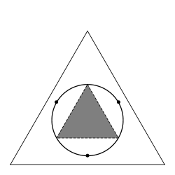
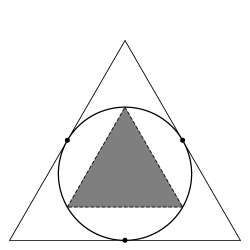
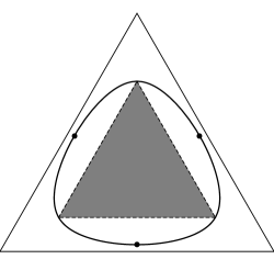
Figure 1: These figures show boundaries of $\tilde{\mathcal{F}}_{\theta_{0}}^{(n)}:=\left\{(F_{11},F_{22},F_{33})\mid\,F\in J^{(U)^{-1/2}}\mathcal{F}_{\theta_{0}}^{(n)}J^{(U)^{-1/2}},\,{\rm Tr}\,F=n^{2}+2n\right\}$, where $\mathcal{F}_{\theta_{0}}^{(n)}$ is the set of classical Fisher information matrices for three-dimensional parametric unitary channel models $\left\{\Gamma_{\theta}^{\otimes n}:\mathcal{B}(\mathbb{C}^{2})\to\mathcal{B}(\mathbb{C}^{2})\mid\,\theta\in\Theta\subset\mathbb{R}^{3}\right\}$ for $n=2$ (top-left), $n=3$ (top-right), $n=4$ (bottom-left), and $n=5$ (bottom-right). The inner triangles painted in gray indicate classical Fisher information matrices that can be realized by using the randomized channel measurements given in Theorem 7 for $n=3,4,5$. For $n=2$, the inner triangle is same as $\tilde{\mathcal{F}}_{\theta_{0}}^{(n)}$, and it is realized by using randomized channel measurements given in Theorem 11. The curves surrounding the inner triangles are the boundaries of $\tilde{\mathcal{F}}_{\theta_{0}}^{(n)}$ for $n=3,4,5$. The three black dots correspond to optimal channel measurements when $d=2$ and weight matrix $W=J_{\theta_{0}}^{(U)}$ given in Theorem 8.

6 Conclusion

In this paper, we defined a Fisher information matrix $J_{\theta_{0}}^{(U)}$ at $\theta_{0}\in\Theta$ for the $SU(2)$ channel model $\mathcal{G}^{(n)}:=\left\{\Gamma_{\theta}^{\otimes n}:\rho\mapsto U_{\theta}^{\otimes n}\rho U_{\theta}^{*\otimes n}\mid\theta\in\Theta\subset\mathbb{R}^{d}\right\}$ with $d=1,2,3$, and we showed a matrix inequality $n^{2}V_{\theta_{0}}[\psi,M,\hat{\theta}]\geq J_{\theta_{0}}^{(U)}$ for covariance matrix $V_{\theta_{0}}[\psi,M,\hat{\theta}]$ of locally unbiased estimator $\left(\psi,M,\hat{\theta}\right)$. When $n=1$, this equality is achievable by a maximally entangled input state. When $n=2$ and $d=2$, this equality is achievable by a pure state input given in Theorem 4 without an ancilla Hilbert space.

When $d=3$, we proved a Gill and Massar type inequality $(n^{2}+2n){\rm Tr}\,WV_{\theta_{0}}^{(n)}[\rho,M,\hat{\theta}]\geq c_{\theta_{0},W}$ with a lower bound $c_{\theta_{0},W}:=\left({\rm Tr}\,\sqrt{J_{\theta_{0}}^{(U)^{-1/2}}WJ_{\theta_{0}}^{(U)^{-1/2}}}\right)^{2}$ for a $d\times d$ real positive matrix $W$. When $n\geq\max\left\{3,\frac{\sqrt{w_{2}}+\sqrt{w_{3}}}{\sqrt{w_{1}}}-1\right\}$, the lower bound $c_{\theta_{0},W}$ is achievable by using a randomized channel measurement without an ancilla Hilbert space, where $w_{1},w_{2},w_{3}$ are eigenvalues of $\tilde{W}:=J_{\theta_{0}}^{(U)^{-1/2}}WJ_{\theta_{0}}^{(U)^{-1/2}}$ such that $0\leq w_{1}\leq w_{2}\leq w_{3}$. When $d=3$ and $n=2$, more informative and achievable bounds were obtained in Theorem 10.

When $d=2$ we proved $2\left\lfloor\frac{n^{2}+2n}{2}\right\rfloor{\rm Tr}\,WV_{\theta_{0}}^{(n)}[\rho,M,\hat{\theta}]\geq c_{\theta_{0},W}$, and the equality is achievable if $W=J_{\theta_{0}}^{(U)}$. For an arbitrary weight $W$ and $d=2$, the lower bound $c_{\theta_{0},W}$ is asymptotically achievable by using a sequence of randomized channel measurements.

There are many examples of $SU(2)$ structures in nature. For example, a three dimensional magnetic field has $SU(2)$ structures, and its estimation has been well studied[21, 22, 23]. The results of this paper could update these research in that it addresses general arbitrary weights and general strategies. This paper is limited to the $SU(2)$ channel model among channel estimation. However, as can be seen from the Fig. 1, the $SU(2)$ model estimation with arbitrary weights has a sufficiently complex structure. To extend the theory of this paper to the $SU(d)$ channel model with $d\geq 3$ seems to be a very challenging problem.

Appendices

Appendix A Generalized purification

In this appendix, we show a generalized purification as follows.

Lemma 12.

For any quantum state $\rho\in\mathcal{S}(\mathcal{H}\otimes\mathcal{H}_{a})$ on a tensor product Hilbert space $\mathcal{H}\otimes\mathcal{H}_{a}$ of two Hilbert spaces $\mathcal{H}$ and $\mathcal{H}_{a}$, there exists another Hilbert space $\mathcal{H}_{b}$ and a pure state $\left|\psi\right\rangle\left\langle\psi\right|\in\mathcal{S}(\mathcal{H}\otimes\mathcal{H}_{b})$ on $\mathcal{H}\otimes\mathcal{H}_{b}$ and a quantum channel $\Lambda:\mathcal{B}(\mathcal{H}_{b})\to\mathcal{B}(\mathcal{H}_{a})$ such that

$${\rm id}_{\mathcal{H}}\otimes\Lambda(\left|\psi\right\rangle\left\langle\psi\right|)=\rho$$ (82)

and

$$\dim\mathcal{H}_{b}\leq\dim\mathcal{H}.$$ (83)

Proof.

Let

$$\rho=\sum_{i=1}^{r}p_{i}\left|e_{i}\right\rangle\left\langle e_{i}\right|$$

be a spectral decomposition of $\rho$ with an orthonormal basis $\left\{\left|e_{i}\right\rangle\right\}_{i}$ of $\mathcal{H}\otimes\mathcal{H}_{a}$ and non-negative values $\left\{p_{i}\right\}_{i}$ such that $\sum_{i}p_{i}=1$. Let us consider a vector

$$\left|\psi^{\prime}\right\rangle=\sum_{i=1}^{r}\sqrt{p_{i}}\left|e_{i}\right\rangle\left|e_{i}^{\prime}\right\rangle\in\mathcal{H}\otimes\mathcal{H}_{a}\otimes\mathcal{H}_{a}^{\prime}$$

with an orthonormal basis $\left\{\left|e_{i}^{\prime}\right\rangle\right\}_{i=1}^{r}\subset\mathcal{H}_{a}^{\prime}$ of a Hilbert space $\mathcal{H}_{a}^{\prime}$ ($\dim\mathcal{H}_{a}^{\prime}=r$). Note that ${\rm Tr}_{\mathcal{H}_{a}^{\prime}}\left|\psi^{\prime}\right\rangle\left\langle\psi^{\prime}\right|=\rho$. By using the singular value decomposition, $\left|\psi^{\prime}\right\rangle$ can be decomposed to

$$\left|\psi^{\prime}\right\rangle=\sum_{k=1}^{s}\sqrt{q_{k}}\left|f_{k}\right\rangle\left|f_{k}^{\prime}\right\rangle,$$

where $\left\{\left|f_{k}\right\rangle\right\}_{k=1}^{s}\subset\mathcal{H}$ and $\left\{\left|f_{k}^{\prime}\right\rangle\right\}_{k=1}^{s}\subset\mathcal{H}_{a}\otimes\mathcal{H}_{a}^{\prime}$ are orthonormal sets, and $\left\{q_{k}\right\}_{k}$ are positive values such that $\sum_{k=1}^{s}q_{k}=1$ with $s\leq\dim\mathcal{H}$.

Let $\mathcal{H}_{b}$ be an $s$-dimensional Hilbert space with an orthonormal basis $\left\{\left|g_{k}\right\rangle\right\}_{k=1}^{s}\subset\mathcal{H}_{b}$, and let $E:\mathcal{H}_{b}\rightarrow\mathcal{H}_{a}\otimes\mathcal{H}_{a}^{\prime}$ be an embedding such that $E\left|g_{k}\right\rangle=\left|f_{k}^{\prime}\right\rangle$ for $k=1,\dots,s$. It can be seen that a vector

$$\left|\psi\right\rangle=\sum_{k=1}^{s}\sqrt{q_{k}}\left|f_{k}\right\rangle\left|g_{k}\right\rangle\in\mathcal{H}\otimes\mathcal{H}_{b}$$

and a channel $\Lambda$ defined by

$$\Lambda(B)={\rm Tr}_{\mathcal{H}_{a}^{\prime}}EBE^{*}\qquad(B\in\mathcal{B}(\mathcal{H}_{b}))$$

satisfy (82). In fact,

$${\rm id}_{\mathcal{H}}\otimes\Lambda(\left|\psi\right\rangle\left\langle\psi\right|) ={\rm Tr}_{\mathcal{H}_{a}^{\prime}}(I\otimes E)\left|\psi\right\rangle\left\langle\psi\right|(I\otimes E)^{*}$$

$$={\rm Tr}_{\mathcal{H}_{a}^{\prime}}\left|\psi^{\prime}\right\rangle\left\langle\psi^{\prime}\right|=\rho.$$

∎

Appendix B SLD bound and Holevo bound

Let $\left\{\rho_{\theta}\in\mathcal{S}(\mathcal{H})\mid\,\theta\in\Theta\subset\mathbb{R}^{d}\right\}$ be a quantum statistical model on a finite dimensional Hilbert space $\mathcal{H}$. It is known that any locally unbiased estimator $(M,\hat{\theta})$ at $\theta_{0}\in\Theta$ satisfies inequalities

$${\rm Tr}\,WV_{\theta_{0}}[M,\hat{\theta}] \geq C_{\theta_{0},W}^{(H)}$$ (84)

$$\geq C_{\theta_{0},W}^{(S)},$$ (85)

where $C_{\theta_{0},W}^{(H)}$ is the Holevo bound for a weight $W>0$ defined by

$$C_{\theta_{0},W}^{(H)} :=\min_{B}\left\{\left.{\rm Tr}\,WZ(B)+{\rm Tr}\,\left|\sqrt{W}{\rm Im}Z(B)\sqrt{W}\right|\right|Z_{ij}(B)={\rm Tr}\,\rho_{\theta_{0}}B_{j}B_{i},\right.$$ (86)

$$\qquad\left.B_{1},\dots,B_{d}\text{ are Hermitian operators on $\mathcal{H}$ such that }{\rm Tr}\,\partial_{i}\rho_{\theta_{0}}B_{j}=\delta_{ij}\right\},$$ (87)

and $C_{\theta_{0},W}^{(S)}$ is the SLD bound defined by ${\rm Tr}\,WJ_{\theta_{0}}^{(S)^{-1}}$ with the SLD Fisher information matrix $J_{\theta_{0}}^{(S)}$. In general, the equation of (84) is not achievable, and Nagaoka-Hayashi bound and conic programming bound have been proposed as more improved lower bounds [24, 25]. For pure state models treated in this paper, the equation of (84) is achievable (see Appendix C). The following lemma is known as a relation between the Holevo bound and the SLD bound.

Lemma 13.

The Holevo bound and the SLD bound of any quantum statistical model $\left\{\rho_{\theta}\in\mathcal{S}(\mathcal{H})\mid\,\theta\in\Theta\subset\mathbb{R}^{d}\right\}$ satisfy

$$C_{\theta_{0},W}^{(H)}=C_{\theta_{0},W}^{(S)}$$

for any weight $W$ if and only if

$${\rm Tr}\,\rho_{\theta_{0}}L_{\theta_{0},i}L_{\theta_{0},j}\in\mathbb{R}$$

for $1\leq i,j\leq d$, where $L_{\theta_{0},i}$ is the SLD at $\theta_{0}\in\Theta$ in the $i$th direction.

Proof.

We can see that observable $B_{i}$ in (87) satisfies

$${\rm Tr}\,\partial_{i}\rho_{\theta_{0}}B_{j}={\rm Re}{\rm Tr}\,\rho_{\theta_{0}}L_{\theta_{0},i}B_{j}=\delta_{ij}.$$

It can be seen that

$$C_{\theta_{0},W}^{(S)} =\min_{B}\left\{\left.{\rm Tr}\,WZ(B)\right|Z_{ij}(B)={\rm Tr}\,\rho_{\theta_{0}}B_{j}B_{i},\right.$$ (88)

$$\qquad\left.B_{1},\dots,B_{d}\text{ are Hermitian operators on $\mathcal{H}$ such that }{\rm Tr}\,\partial_{i}\rho_{\theta_{0}}B_{j}=\delta_{ij}\right\},$$ (89)

and the minimum is achieved by observables defined by

$$B_{i}^{(S)}:=\sum_{j=1}^{d}\left[J_{\theta}^{(S)^{-1}}\right]^{ij}L_{\theta_{0},j}$$

because

$${\rm Re}Z(B)_{ij} ={\rm Re}{\rm Tr}\,\rho_{\theta_{0}}\left(B_{j}^{(S)}+K_{j}\right)\left(B_{i}^{(S)}+K_{i}\right)$$

$$={\rm Re}{\rm Tr}\,\rho_{\theta_{0}}B_{j}^{(S)}B_{i}^{(S)}+{\rm Re}{\rm Tr}\,\rho_{\theta_{0}}K_{j}K_{i}$$

$$={\rm Re}Z(B^{(S)})_{ij}+{\rm Re}Z(K)_{ij}$$

$$={\rm Re}\left[J_{\theta}^{(S)^{-1}}\right]_{ij}+{\rm Re}Z(K)_{ij},$$

where $K_{i}=B_{i}-B_{i}^{(S)}$. Therefore $C_{\theta_{0},W}^{(S)}=C_{\theta_{0},W}^{(H)}$ if and only if ${\rm Tr}\,\left|\sqrt{W}{\rm Im}Z(B^{(S)})\sqrt{W}\right|=0$. This condition is equivalent to ${\rm Tr}\,\rho_{\theta_{0}}L_{\theta_{0},i}L_{\theta_{0},j}\in\mathbb{R}$. ∎

Appendix C Holevo bound for pure state model

Theorem 14.

Let $\left\{\rho_{\theta}\mid\,\theta\in\Theta\subset\mathbb{R}^{d}\right\}$ be a quantum statistical model comprising pure states on a finite dimensional Hilbert space $\mathcal{H}$, and let $C_{\theta_{0},W}^{(H)}$ be the Holevo bound at $\theta_{0}\in\Theta$ for a given weight $W>0$. There exist a locally unbiased estimator $\left(M,\hat{\theta}\right)$ at $\theta_{0}\in\Theta$ such that

$${\rm Tr}\,WV_{\theta_{0}}[M,\hat{\theta}] ={\rm Tr}\,WJ_{\theta_{0}}^{(C,M)^{-1}}=C_{\theta_{0},W}^{(H)}$$ (90)

$$\geq C_{\theta_{0},W}^{(S)},$$ (91)

where $J_{\theta_{0}}^{(C,M)}$ is the classical Fisher information matrix with restrict to the POVM $M$.

The inequality (91) for any $W>0$ implies

$$J_{\theta_{0}}^{(C)}(M)\leq J_{\theta_{0}}^{(S)},$$ (92)

and the equality is achievable by a projection valued measurement $M$ if and only if SLDs $\left\{L_{\theta_{0},i}\right\}_{i=1}^{d}$ satisfy

$${\rm Tr}\,\rho_{\theta_{0}}L_{\theta_{0},i}L_{\theta_{0},j}\in\mathbb{R}$$ (93)

for $1\leq i,j\leq d$.

Proof.

Let $B_{1},\dots,B_{d}$ be observables that attain the minimum in (87), and let $\left|\xi_{i}\right\rangle:=B_{i}\left|\psi\right\rangle\in\mathcal{H}$ be vectors for $1\leq i\leq d$ with $\left|\psi\right\rangle\in\mathcal{H}$ such that $\rho_{\theta_{0}}:=\left|\psi\right\rangle\left\langle\psi\right|$. Let

$$\hat{Z}:=\sqrt{W}^{-1}\left|\sqrt{W}{\rm Im}Z(B)\sqrt{W}\right|\sqrt{W}^{-1}-\sqrt{-1}{\rm Im}Z(B)$$

be a positive-semidefinite matrix, and let $\hat{r}={\rm rank}\hat{Z}$. There exits a Hilbert space $\hat{\mathcal{H}}=\mathbb{C}^{\hat{r}+1}$ and vectors $\left|\hat{\psi}\right\rangle,\left|\hat{\xi}_{1}\right\rangle,\dots,\left|\hat{\xi}_{d}\right\rangle\in\mathcal{H}_{a}$ such that

$$\left\langle\hat{\xi}_{i}\mid\hat{\xi}_{j}\right\rangle =\hat{Z}_{ij}\qquad(1\leq i,j\leq d),$$

$$\left\langle\hat{\psi}\mid\hat{\xi}_{i}\right\rangle =0\qquad(1\leq i\leq d),$$

$$\left\langle\hat{\psi}\mid\hat{\psi}\right\rangle =1.$$

Let

$$\left|\tilde{\xi}_{i}\right\rangle :=\left|\xi_{i}\right\rangle\otimes\left|\hat{\psi}\right\rangle+\left|\psi\right\rangle\otimes\left|\hat{\xi}_{i}\right\rangle\qquad(1\leq i\leq d),$$

$$\left|\tilde{\psi}\right\rangle :=\left|\psi\right\rangle\otimes\left|\hat{\psi}\right\rangle$$

be vectors in $\mathcal{H}\otimes\hat{\mathcal{H}}$. Because $\left\langle\tilde{\psi}\mid\tilde{\xi}_{i}\right\rangle(=0)$ and $\left\langle\tilde{\xi}_{i}\mid\tilde{\xi}_{j}\right\rangle(={\rm Re}Z(B)_{ji}+{\rm Re}\hat{Z}_{ji})$ are all real, there exist an orthonormal basis $\left\{\left|\tilde{e}_{k}\right\rangle\right\}_{k=1}^{\dim\mathcal{H}\otimes\hat{\mathcal{H}}}$ of $\mathcal{H}\otimes\hat{\mathcal{H}}$ such that $\left\langle\tilde{e}_{k}\mid\tilde{\psi}\right\rangle$ and $\left\langle\tilde{e}_{k}\mid\tilde{\xi}_{i}\right\rangle$ are all real, and that $\left\langle\tilde{e}_{k}\mid\tilde{\psi}\right\rangle\not=0$ for all $k$. Let

$$\tilde{T}_{i}:=\theta_{0}^{i}I_{\mathcal{H}\otimes\hat{\mathcal{H}}}+\sum_{k=1}^{\dim\mathcal{H}\otimes\hat{\mathcal{H}}}\frac{\left\langle\tilde{e}_{k}\mid\tilde{\xi}_{i}\right\rangle}{\left\langle\tilde{e}_{k}\mid\tilde{\psi}\right\rangle}\left|\tilde{e}_{k}\right\rangle\left\langle\tilde{e}_{k}\right|\qquad(1\leq i\leq d),$$

be observables on $\mathcal{H}\otimes\hat{\mathcal{H}}$. Then $\tilde{T}_{1},\dots,\tilde{T}_{d}$ are simultaneously measurable, and satisfy the local unbiasedness condition:

$${\rm Tr}\,\left(\rho_{\theta_{0}}\otimes\left|\hat{\psi}\right\rangle\left\langle\hat{\psi}\right|\right)\tilde{T}_{i}=\left\langle\tilde{\psi}\right|\tilde{T}_{i}\left|\tilde{\psi}\right\rangle=\theta_{0}^{i}$$

and

$${\rm Tr}\,\left(\partial_{i}\rho_{\theta_{0}}\otimes\left|\hat{\psi}\right\rangle\left\langle\hat{\psi}\right|\right)\tilde{T}_{j}={\rm Re}\left\langle\tilde{l}_{i}\right|\tilde{T}_{j}\left|\tilde{\psi}\right\rangle=\delta_{ij},$$

where

$$\left|\tilde{l}_{i}\right\rangle=\left(L_{\theta_{0},i}\left|\psi\right\rangle\right)\otimes\left|\hat{\psi}\right\rangle.$$

Further they satisfy

$$V_{\theta_{0}}[\tilde{T}]_{ij} ={\rm Tr}\,\left(\rho_{\theta_{0}}\otimes\left|\hat{\psi}\right\rangle\left\langle\hat{\psi}\right|\right)\left(\tilde{T}_{i}-\theta_{0}^{i}I_{\mathcal{H}\otimes\hat{\mathcal{H}}}\right)\left(\tilde{T}_{j}-\theta_{0}^{j}I_{\mathcal{H}\otimes\hat{\mathcal{H}}}\right)$$

$$=\left\langle\tilde{\xi}_{i}\mid\tilde{\xi}_{j}\right\rangle={\rm Re}Z(B)_{ji}+{\rm Re}\hat{Z}_{ji}$$

$$=\left[{\rm Re}Z(B)+\sqrt{W}^{-1}\left|\sqrt{W}{\rm Im}Z(B)\sqrt{W}\right|\sqrt{W}^{-1}\right]_{ji}.$$

This implies ${\rm Tr}\,WV_{\theta_{0}}[\tilde{T}]=C_{\theta_{0},W}^{(H)}$.

The proof of the equality achievement condition for (92) is given in Lemma 13. Note that when ${\rm Tr}\,\rho_{\theta_{0}}L_{\theta_{0},i}L_{\theta_{0},j}\in\mathbb{R}$ for $1\leq i,j\leq d$, ${\rm Im}Z(B)=0$ and $\dim\hat{\mathcal{H}}=1$. Thus, $\left\{\tilde{T}_{i}\right\}_{i=1}^{d}$ are observables on $\mathcal{H}$, and they correspond to a projection valued measurement on $\mathcal{H}$. ∎

Appendix D Numerical calculations for the curves in Figure 1

In this appendix, we details about the numerical calculations to obtain the curves in Figure 1. Without loss of generality, we can assume $X_{1},X_{2},X_{3}$ are Pauli matrices and $J_{\theta_{0}}^{(U)}=I$. To reveal the boundary of the convex set $\tilde{\mathcal{F}}_{\theta_{0}}^{(n)}$, we calculate

$$F^{(i)}(t):=\mathop{\rm arg~{}max}\limits_{F\in\mathcal{F}_{\theta_{0}}^{(n)}}{\rm Tr}\,H_{t}^{(i)}F$$ (94)

numerically for $t\in[0,1]$ and $i=1,2,3$, where $H_{t}^{(1)}={\rm diag}(0,t,1-t)$, $H_{t}^{(2)}={\rm diag}(1-t,0,t)$, $H_{t}^{(3)}={\rm diag}(t,1-t,0)$. We can see that $F^{(i)}(t)$ corresponds to a point on the boundary of $\tilde{\mathcal{F}}_{\theta_{0}}^{(n)}$. To calculate $F^{(3)}(t)$, we compute an unit eigenvector $\left|t\right\rangle$ of $(tX_{1}^{(n)^{2}}+(1-t)X_{2}^{(n)^{2}})\otimes I$ with respect to the maximum eigenvalue with a $2\times 2$ identity matrix $I$. Finally, we check that $\left\langle t\right|X_{i}^{(n)}X_{j}^{(n)}\otimes I\left|t\right\rangle$ is a real value and $\left\langle t\right|X_{i}^{(n)}\otimes I\left|t\right\rangle=0$ for $1\leq i,j\leq 3$ to verify $\left|t\right\rangle\in\mathcal{A}_{\theta_{0}}^{(n)}$, then we obtain $F^{(3)}(t)=\left[\left\langle t\right|X_{i}^{(n)}X_{j}^{(n)}\otimes I\left|t\right\rangle\right]_{ij}$. The calculation of $F^{(1)}(t)$ and $F^{(2)}(t)$ are similar.

References

• [1] M. Szczykulska, T. Baumgratz, and A. Datta, โ€œMulti-parameter quantum metrology,โ€ Advances in Physics: X, 1(4), 621โ€“639 (2016).
• [2] J. Liu, H. Yuan, X. M. Lu, and X. Wang, โ€œQuantum Fisher information matrix and multiparameter estimation,โ€ J. Phys. A: Math. Theor. 53 023001 (2020).
• [3] R. Demkowicz-Dobrzanรฉski, W. Goรฉrecki, and M. Guลฃฤƒ, โ€œMulti-parameter estimation beyond quantum Fisher information,โ€ J. Phys. A: Math. Theor. 53 363001 (2020).
• [4] F. Albarelli, M. Barbieri, M.G. Genoni, and I. Gianani, โ€œA perspective on multiparameter quantum metrology: From theoretical tools to applications in quantum imaging,โ€ Physics Letters A,Volume 384, Issue 12, (2020).
• [5] A. S. Holevo, โ€œProbabilistic and Statistical Aspects of Quantum Theory,โ€ (2nd English edition) (Edizioni della Normale, Pisa., 2011).
• [6] R. D. Gill and S. Massar, โ€œState estimation for large ensembles,โ€ Physical Review A, 61, 042312 (2000).
• [7] M. Hayashi, โ€œA linear programming approach to attainable Cramรฉr-Rao type bounds,โ€ Quantum Communication, Computing, and Measurement 99-108. Plenum, New York (1997).
• [8] K. Yamagata, โ€œEffciency of quantum state tomography for qubits,โ€ Int. J. Quant. Inform., 9, 1167 (2011).
• [9] A. Fujiwara, โ€œEstimation of SU(2) operation and dense coding: An information geometric approach,โ€ Phys. Rev. A 65, 012316 (2002).
• [10] H. Imai, and A. Fujiwara, โ€œGeometry of optimal estimation scheme for SU(D) channels,โ€ J. Phys. A: Math. Theor. 40 4391 (2007).
• [11] M. Hayashi, โ€œParallel treatment of estimation of SU(2) and phase estimation,โ€ Phys. Lett. A 354, 183-189 (2006).
• [12] J. Kahn, โ€œFast rate estimation of a unitary operation in SU(d),โ€ Physical Review A 75(2) (2006).
• [13] A. Fujiwara, โ€œStrong consistency and asymptotic efficiency for adaptive quantum estimation problems,โ€ Journal of Physics A: Mathematical and Theoretical 44(7) 079501-079501 (2011).
• [14] W. Goรฉrecki and R. Demkowicz-Dobrzanรฉski, โ€œMultiparameter quantum metrology in the Heisenberg limit regime: Many-repetition scenario versus full optimization,โ€ Phys. Rev. A 106, 012424 (2022).
• [15] K. Matsumoto, โ€œA new approach to the Cramรฉr-Rao-type bound of the pure-state model,โ€ J. Phys. A 35 3111-3123. MR1913859 (2002).
• [16] H. Yuan and C. F. Fung, โ€œFidelity and Fisher information on quantum channels,โ€ New J. Phys. 19 113039 (2017).
• [17] Y. Chen and H. Yuan, โ€œMaximal quantum Fisher information matrix,โ€ New J. Phys. 19 063023 (2017).
• [18] W. Goรฉrecki, S. Zhou, L. Jiang, and R. Demkowicz-Dobrzanรฉski, โ€œOptimal probes and error-correction schemes in multi-parameter quantum metrology,โ€ Quantum 4, 288 (2020).
• [19] W. Goรฉrecki and R. Demkowicz-Dobrzanรฉski, โ€œMultiple-Phase Quantum Interferometry: Real and Apparent Gains of Measuring All the Phases Simultaneously,โ€ Phys. Rev. Lett. 128, 040504 (2022).
• [20] F. Albarelli and R. Demkowicz-Dobrzanรฉski, โ€œProbe Incompatibility in Multiparameter Noisy Quantum Metrology,โ€ Phys. Rev. X 12, 011039 (2022).
• [21] T. Baumgratz and A. Datta, โ€œQuantum Enhanced Estimation of a Multidimensional Field,โ€ Phys. Rev. Lett. 116, 030801 (2016).
• [22] H. Yuan, โ€œSequential Feedback Scheme Outperforms the Parallel Scheme for Hamiltonian Parameter Estimation,โ€ Phys. Rev. Lett. 117, 160801 (2016).
• [23] Z. Hou, Z. Zhang, G. Xiang, C. Li, G. Guo, H. Chen, L. Liu, and H. Yuan, โ€œMinimal Tradeoff and Ultimate Precision Limit of Multiparameter Quantum Magnetometry under the Parallel Scheme,โ€ Phys. Rev. Lett. 125, 020501 (2020).
• [24] L. O. Conlon, J. Suzuki, P. K. Lam, S. M. Assad, โ€œEfficient computation of the Nagaokaโ€“Hayashi bound for multiparameter estimation with separable measurements,โ€ npj Quantum Information 7, 110 (2021).
• [25] M. Hayashi and Y. Ouyang, โ€œTight Cramรฉr-Rao type bounds for multiparameter quantum metrology through conic programming,โ€ Quantum 7, 1094 (2023).