Window convolution of the galaxy clustering bispectrum

Abstract

In galaxy survey analysis, the observed clustering statistics do not directly match theoretical predictions but rather have been processed by a window function that arises from the survey geometry including the sky footprint, redshift-dependent background number density and systematic weights. While window convolution of the power spectrum is well studied, for the bispectrum with a larger number of degrees of freedom, it poses a significant numerical and computational challenge. In this work, we consider the effect of the survey window in the tripolar spherical harmonic decomposition of the bispectrum and lay down a formal procedure for their convolution via a series expansion of configuration-space three-point correlation functions, which was first proposed by Sugiyama et al. (2019). We then provide a linear algebra formulation of the full window convolution, where an unwindowed bispectrum model vector can be directly premultiplied by a window matrix specific to each survey geometry. To validate the pipeline, we focus on the Dark Energy Spectroscopic Instrument (DESI) Data Release 1 (DR1) luminous red galaxy (LRG) sample in the South Galactic Cap (SGC) in the redshift bin $$0.4$\leqslant z\leqslant$0.6$$. We first perform convergence checks on the measurement of the window function from discrete random catalogues, and then investigate the convergence of the window convolution series expansion truncated at a finite of number of terms as well as the performance of the window matrix. This work highlights the differences in window convolution between the power spectrum and bispectrum, and provides a streamlined pipeline for the latter for current surveys such as DESI and the Euclid mission.

1 Introduction

Measurements of cosmological observables usually cannot be directly compared to their theoretical predictions not only because they are noisy realisations, but also because they have been processed by a window function that filters the underlying signal. In galaxy clustering analysis, the window function encodes the survey geometry and includes selection functions of the background number density, as well as any weights applied to compensate for systematic effects or to enhance the signal-to-noise ratio [1]. For correlation functions in configuration space, their window functions are locally multiplicative and are thus relatively easy to account for; in Fourier space, the window function instead convolves with the polyspectra such as the power spectrum and bispectrum. This mixes clustering modes on different scales, and modulates both the shape and the amplitude of the clustering statistics [2]; moreover, since the window function itself is typically anisotropic, it couples to anisotropies arising from redshift-space distortions (RSD) and the Alcock–Paczyński (AP) effect [3, 4], and therefore must be accounted for in their statistical analysis.

One way to disentangle the window function is to deconvolve it from clustering statistics such as the quadratic and cubic (near-)optimal estimators of the power spectrum and bispectrum [e.g. 5, 6, 7, 8, 9, 10, 11], which are numerically difficult to obtain and require the inversion and differentiation of covariance and Fisher matrices at the map pixel level. Fundamentally, deconvolution is an inverse operation (akin to division in configuration space), and so it may suffer from ill-conditioning especially with noisy estimates of clustering statistics.

The alternative approach, which has become standard for the analysis of the galaxy clustering power spectrum, is to forward model the window function by performing convolution as multiplication in configuration space [12, 13]. This is particularly advantageous for compressed clustering statistics such as Legendre multipoles of the correlation function or the power spectrum ($\xi_{L}$ or $P_{L}$), where the window function multipoles $Q_{L}$ can be measured in a similar way, and multipoles in configuration and Fourier spaces are related through the Hankel transform. In addition, for predefined binning, the entire procedure is a combination of linear algebra operations and can be cast as matrix multiplications for fast computation [14, 15].

Although the treatment of the window function for power spectrum has been standardised this way in recent analyses of the 6-degree Field Galaxy Redshift Survey (6dFGRS), the Baryon Oscillation Spectroscopic Survey (BOSS) and its extension eBOSS [e.g. 13, 16, 14, 17, 18, 19], it remains challenging for three-point clustering statistics in Fourier space, where perturbative models of the bispectrum such as the effective field theory of large-scale structure are presented [e.g. 20, 21, 22, 23, 24, 25, 26]. This is because higher-order clustering statistics have many more degrees of freedom; for instance, whereas the power spectrum is a function of a single wavevector $\mathbf{k}$ under the assumption of statistical homogeneity, the bispectrum is a function of two wavevectors defining a closed triangle also under statistical homogeneity.

In the analysis of BOSS galaxy catalogues, refs. [27, 28] have replaced the bispectrum window convolution with convolution of the two-point window function with each power spectrum kernel in the bispectrum model; this is a mathematically inequivalent procedure and an inaccurate approximation on large scales. More recently, ref. [29] has suggested the deployment of deep neural networks to ‘learn’ the effect of the window function on the bispectrum from a large suite of training simulations; aside from the computational cost of this approach which needs to be repeated for each window function, this proof-of-concept study has had to assume a relation between the unwindowed and windowed bispectra that is a local and isotropic response function in Fourier space. For the commonly considered Scoccimarro bispectrum multipoles $\mathop{}\!B_{L}^{M}{\mathopen{}\mathclose{{}\left(k_{1},k_{2},k_{3}}\right)}$ in the basis proposed by ref. [30], ref. [31] has laid down the analytical expressions for the window convolution, but the window function is decomposed into a much larger set of multipole components with five additional spherical degrees $\ell$, each requiring the summation over multiple spherical orders $m$. This induces a significant computational cost, even when they can be recast in a form amenable to the fast Fourier transform (FFT).

In this work, we consider an alternative decomposition of three-point clustering statistics in the tripolar spherical harmonic (TripoSH) basis, which was first proposed by ref. [32]. In this decomposition, the third internal angle (or equivalently, its corresponding side) of the bispectrum triangles is integrated out, resulting in multipoles $\mathop{}\!B_{\ell_{1}\ell_{2}L}{\mathopen{}\mathclose{{}\left(k_{1},k_{2}}\right)}$ with only two wavenumbers and two additional spherical degrees $\ell_{1},\ell_{2}$. In contrast to the Scoccimarro multipoles which have three wavenumbers, this is a form of data dimensionality reduction, as the bispectrum multipoles are now effectively two-dimensional rather than three-dimensional quantities, which reduces the computational cost, especially for covariance matrix estimation. The three-point correlation function (3PCF) admits a similar expansion into multipoles that are related to the bispectrum multipoles through a double spherical Bessel transform. More crucially, as demonstrated in ref. [32] and discussed later in this work, the window function in the TripoSH formulation can be decomposed into similar multipoles that can be measured in the same way as for the bispectrum and 3PCF multipoles using FFTs. The full window convolution procedure is then analogous to that of two-point clustering statistics as laid down by refs. [12, 13], where in configuration space the windowed 3PCF multipoles are series expansions in terms of the window function multipoles and the unwindowed 3PCF multipoles. Whereas ref. [32] only considers the leading-order term in the series and ref. [33] focuses on the configuration space, we investigate the importance of non-leading-order terms here in Fourier space. Moreover, this approach also allows us to propose a simple linear algebra formulation where a given unwindowed bispectrum model vector is premultiplied by a window matrix, the result of which can then be compared with the measured data vector as for the power spectrum [15].

This article proceeds as follows. We first introduce the TripoSH decomposition and write down the FFT-based estimators proposed by ref. [32] in section 2. We then lay out the window convolution procedure in section 3, including the numerical implementation of the double spherical Bessel transform required to convert between Fourier- and configuration-space statistics and the linear algebra formulation of a window matrix. In a series of validation tests detailed in section 4, we discuss the convergence of window function measurements with respect to the sampling of the number density field, as well as truncation and approximations adopted in the window convolution formula. We will highlight some technical differences in window convolution between three-point and two-point clustering statistics as well as between Fourier and configuration space, before drawing a conclusion in section 5.

Throughout this work, we will use our publicly available code Triumvirate to measure all three-point clustering statistics including the window function and to perform window convolution [34].

2 Tripolar spherical harmonic decomposition

Given a catalogue of discrete particles, one could assign their positions $\mathbf{x}$ to a regular mesh grid of cells to compute fluctuations in the number density field $n(\mathbf{x})$ with any weights $\mathop{}\!w{\mathopen{}\mathclose{{}\left(\mathbf{x}}\right)}$ (such as the Feldman–Kaiser–Peacock scheme [1]),

$$\mathop{}\!\delta{n}{\mathopen{}\mathclose{{}\left(\mathbf{x}}\right)}=\mathop{}\!w{\mathopen{}\mathclose{{}\left(\mathbf{x}}\right)}\quantity[\mathop{}\!n{\mathopen{}\mathclose{{}\left(\mathbf{x}}\right)}-\mathop{}\!\bar{n}{\mathopen{}\mathclose{{}\left(\mathbf{x}}\right)}missing]\,.$$ (2.1)

Here the background number density $\mathop{}\!\bar{n}{\mathopen{}\mathclose{{}\left(\mathbf{x}}\right)}$ is constant for a simulation snapshot, and for a galaxy survey catalogue, it may include the selection function and any additional systematic weights to correct for observational effects such as incompleteness. In the latter case, $\mathop{}\!\bar{n}{\mathopen{}\mathclose{{}\left(\mathbf{x}}\right)}$ is typically sampled by a much denser random catalogue but rescaled to match the number density of the data catalogue.

In redshift space where the radial distance to each galaxy is converted from its observed redshift subject to peculiar velocity, clustering statistics such as the 3PCF depends on the line of sight, $\hat{\mathbf{n}}$, in addition to the separation $\mathbf{r}_{1,2}$,

$$\zeta(\mathbf{r}_{1},\mathbf{r}_{2},\hat{\mathbf{n}})=\expectationvalue{\mathop{}\!\delta{\mathopen{}\mathclose{{}\left(\mathbf{x}+\mathbf{r}_{1}}\right)}\mathop{}\!\delta{\mathopen{}\mathclose{{}\left(\mathbf{x}+\mathbf{r}_{2}}\right)}\mathop{}\!\delta{\mathopen{}\mathclose{{}\left(\mathbf{x}}\right)}missing}\,,$$ (2.2)

where $\expectationvalue{\cdot}$ denotes the ensemble average, and $\mathop{}\!\delta{\mathopen{}\mathclose{{}\left(\mathbf{x}}\right)}=\mathop{}\!\delta{n}{\mathopen{}\mathclose{{}\left(\mathbf{x}}\right)}/\mathop{}\!\bar{n}{\mathopen{}\mathclose{{}\left(\mathbf{x}}\right)}$ is the over-density field. In the expression above, we have assumed the end-point definition of the line-of-sight vector $\hat{\mathbf{n}}=\mathbf{x}/\absolutevalue{\mathbf{x}}$ in the local plane-parallel picture.

Analogously, the bispectrum $\mathop{}\!B{\mathopen{}\mathclose{{}\left(\mathbf{k}_{1},\mathbf{k}_{2},\hat{\mathbf{n}}}\right)}$ in Fourier space is a function of two wavevectors $\mathbf{k}_{1}$, $\mathbf{k}_{2}$ and the line-of-sight vector $\hat{\mathbf{n}}$ in the local plane-parallel picture [35, 30]. Under the assumption of parity symmetry, one could construct a basis of functions from three spherical harmonics [32],

$$\mathop{}\!S_{\ell_{1}\ell_{2}L}{\bigl{(}\hat{\mathbf{k}}_{1},\hat{\mathbf{k}}_{2},\hat{\mathbf{n}}\bigr{)}}=H_{\ell_{1}\ell_{2}L}^{-1}\sum_{m_{1}m_{2}M}\matrixquantity(\ell_{1}&\ell_{2}&L\\ m_{1}&m_{2}&M)\mathop{}\!y_{\ell_{1}}^{m_{1}}{\bigl{(}\hat{\mathbf{k}}_{1}\bigr{)}}\mathop{}\!y_{\ell_{2}}^{m_{2}}{\bigl{(}\hat{\mathbf{k}}_{2}\bigr{)}}\mathop{}\!y_{L}^{M}{\mathopen{}\mathclose{{}\left(\hat{\mathbf{n}}}\right)}\,,$$ (2.3)

where the Wigner 3-j factor

$$H_{\ell_{1}\ell_{2}L}=\matrixquantity(\ell_{1}&\ell_{2}&L\\ 0&0&0)$$ (2.4)

enforces $\quantity(\ell_{1}+\ell_{2}+L)\in 2\mathbb{Z}$ to be even, and the spherical harmonics $y_{\ell}^{m}=\sqrt{\ifrac{4\pi}{(2\ell+1)}}Y_{\ell}^{m}$ are normalised such that $y_{0}^{0}\equiv 1$. In this basis, the bispectrum can be expanded as

$$\mathop{}\!B{\mathopen{}\mathclose{{}\left(\mathbf{k}_{1},\mathbf{k}_{2},\hat{\mathbf{n}}}\right)}=\sum_{\ell_{1}+\ell_{2}+L\in 2\mathbb{Z}}\mathop{}\!B_{\ell_{1}\ell_{2}L}{\mathopen{}\mathclose{{}\left(k_{1},k_{2}}\right)}\mathop{}\!S_{\ell_{1}\ell_{2}L}{\bigl{(}\hat{\mathbf{k}}_{1},\hat{\mathbf{k}}_{2},\hat{\mathbf{n}}\bigr{)}}\,,$$ (2.5)

where the multipoles are given by

$$\mathop{}\!B_{\ell_{1}\ell_{2}L}{\mathopen{}\mathclose{{}\left(k_{1},k_{2}}\right)}=N_{\ell_{1}\ell_{2}L}H_{\ell_{1}\ell_{2}L}\sum_{m_{1}m_{2}M}\matrixquantity(\ell_{1}&\ell_{2}&L\\ m_{1}&m_{2}&M)\\ \qquad\times\int\frac{\differential[2]{\hat{\mathbf{k}}_{1}}}{4\uppi}\frac{\differential[2]{\hat{\mathbf{k}}_{2}}}{4\uppi}\frac{\differential[2]{\hat{\mathbf{n}}}}{4\uppi}\mathop{}\!{y_{\ell_{1}}^{m_{1}}}^{\ast}{\bigl{(}\hat{\mathbf{k}}_{1}\bigr{)}}\mathop{}\!{y_{\ell_{2}}^{m_{2}}}^{\ast}{\bigl{(}\hat{\mathbf{k}}_{2}\bigr{)}}\mathop{}\!{y_{L}^{M}}^{\ast}{\mathopen{}\mathclose{{}\left(\hat{\mathbf{n}}}\right)}\mathop{}\!B{\mathopen{}\mathclose{{}\left(\mathbf{k}_{1},\mathbf{k}_{2},\hat{\mathbf{n}}}\right)}$$ (2.6)

with the prefactor $N_{\ell_{1}\ell_{2}L}=(2\ell_{1}+1)(2\ell_{2}+1)(2L+1)$.

Similarly, the 3PCF also admits the same expansion as eqs. 2.5 and 2.3, with its multipoles given by

$$\mathop{}\!\zeta_{\ell_{1}\ell_{2}L}{\mathopen{}\mathclose{{}\left(r_{1},r_{2}}\right)}=N_{\ell_{1}\ell_{2}L}H_{\ell_{1}\ell_{2}L}\sum_{m_{1}m_{2}M}\matrixquantity(\ell_{1}&\ell_{2}&L\\ m_{1}&m_{2}&M)\\ \qquad\times\int\frac{\differential[2]{\hat{\mathbf{r}}_{1}}}{4\uppi}\frac{\differential[2]{\hat{\mathbf{r}}_{2}}}{4\uppi}\frac{\differential[2]{\hat{\mathbf{n}}}}{4\uppi}\mathop{}\!{y_{\ell_{1}}^{m_{1}}}^{\ast}{\bigl{(}\hat{\mathbf{r}}_{1}\bigr{)}}\mathop{}\!{y_{\ell_{2}}^{m_{2}}}^{\ast}{\bigl{(}\hat{\mathbf{r}}_{2}\bigr{)}}\mathop{}\!{y_{L}^{M}}^{\ast}{\mathopen{}\mathclose{{}\left(\hat{\mathbf{n}}}\right)}\mathop{}\!\zeta{\mathopen{}\mathclose{{}\left(\mathbf{r}_{1},\mathbf{r}_{2},\hat{\mathbf{n}}}\right)}\,.$$ (2.7)

These are related to the bispectrum multipoles (eq. 2.6) through a double spherical Bessel transform:

$$\mathop{}\!B_{\ell_{1}\ell_{2}L}{\mathopen{}\mathclose{{}\left(k_{1},k_{2}}\right)} =(4\uppi)^{2}{\mathrm{i}}^{-\ell_{1}-\ell_{2}}\int\differential[2]{r_{1}}r_{1}^{2}\int\differential[2]{r_{2}}r_{2}^{2}\mathop{}\!j_{\ell_{1}}{\mathopen{}\mathclose{{}\left(k_{1}r_{1}}\right)}\mathop{}\!j_{\ell_{2}}{\mathopen{}\mathclose{{}\left(k_{2}r_{2}}\right)}\mathop{}\!\zeta_{\ell_{1}\ell_{2}L}{\mathopen{}\mathclose{{}\left(r_{1},r_{2}}\right)}\,,$$ (2.8a)

$$\mathop{}\!\zeta_{\ell_{1}\ell_{2}L}{\mathopen{}\mathclose{{}\left(r_{1},r_{2}}\right)} =(4\uppi)^{2}{\mathrm{i}}^{\ell_{1}+\ell_{2}}\int\frac{\differential{k_{1}}k_{1}^{2}}{(2\uppi)^{3}}\int\frac{\differential{k_{2}}k_{2}^{2}}{(2\uppi)^{3}}\mathop{}\!j_{\ell_{1}}{\mathopen{}\mathclose{{}\left(k_{1}r_{1}}\right)}\mathop{}\!j_{\ell_{2}}{\mathopen{}\mathclose{{}\left(k_{2}r_{2}}\right)}\mathop{}\!B_{\ell_{1}\ell_{2}L}{\mathopen{}\mathclose{{}\left(k_{1},k_{2}}\right)}\,.$$ (2.8b)

2.1 Estimators of three-point clustering statistics

For convenience, we define the spherical harmonic weighted fluctuation field and its Fourier transform,

$$\mathop{}\!\delta{n}_{\ell}^{m}{\mathopen{}\mathclose{{}\left(\mathbf{x}}\right)}={y_{\ell}^{m}}^{\ast}(\mathbf{x})\delta{n}(\mathbf{x})\mbox{\quad and\quad}\mathop{}\!\delta{n}_{\ell}^{m}{\mathopen{}\mathclose{{}\left(\mathbf{k}}\right)}=\int\differential[3]{\mathbf{k}}\mathrm{e}^{-\mathrm{i}\mathbf{k}\dotproduct\mathbf{x}}\mathop{}\!\delta{n}_{\ell}^{m}{\mathopen{}\mathclose{{}\left(\mathbf{x}}\right)}\,,$$ (2.9)

where the latter can be computed using fast Fourier transform (FFT) with mesh assignment window corrections applied [36, 37]. Assuming the end-point definition of the line of sight, the TripoSH multipoles of the bispectrum and 3PCF in eqs. 2.6 and 2.7 can be cast in a form compatible with FFT [32]:

$$\mathop{}\!\widehat{B}_{\ell_{1}\ell_{2}L}{\mathopen{}\mathclose{{}\left(k_{1},k_{2}}\right)}=I_{3}^{-1}N_{\ell_{1}\ell_{2}L}H_{\ell_{1}\ell_{2}L}\sum_{m_{1}m_{2}M} \matrixquantity(\ell_{1}&\ell_{2}&L\\ m_{1}&m_{2}&M)$$

$$\times\int\differential[3]{\mathbf{x}}\mathop{}\!F_{\ell_{1}}^{m_{1}}{\mathopen{}\mathclose{{}\left(\mathbf{x};k_{1}}\right)}\mathop{}\!F_{\ell_{2}}^{m_{2}}{\mathopen{}\mathclose{{}\left(\mathbf{x};k_{2}}\right)}\mathop{}\!G_{L}^{M}{\mathopen{}\mathclose{{}\left(\mathbf{x}}\right)}\,,$$ (2.10a)

$$\mathop{}\!\widehat{\zeta}_{\ell_{1}\ell_{2}L}{\mathopen{}\mathclose{{}\left(r_{1},r_{2}}\right)}=I_{3}^{-1}N_{\ell_{1}\ell_{2}L}H_{\ell_{1}\ell_{2}L}\sum_{m_{1}m_{2}M} \matrixquantity(\ell_{1}&\ell_{2}&L\\ m_{1}&m_{2}&M)$$

$$\times\int\differential[3]{\mathbf{x}}\mathop{}\!F_{\ell_{1}}^{m_{1}}{\mathopen{}\mathclose{{}\left(\mathbf{x};r_{1}}\right)}\mathop{}\!F_{\ell_{2}}^{m_{2}}{\mathopen{}\mathclose{{}\left(\mathbf{x};r_{2}}\right)}\mathop{}\!G_{L}^{M}{\mathopen{}\mathclose{{}\left(\mathbf{x}}\right)}\,,$$ (2.10b)

with the normalisation constant

$$I_{3}=\int\differential[3]{\mathbf{x}}\mathop{}\!w{\mathopen{}\mathclose{{}\left(\mathbf{x}}\right)}^{3}\mathop{}\!\bar{n}{\mathopen{}\mathclose{{}\left(\mathbf{x}}\right)}^{3}\,.$$ (2.11)

Here the one-point functions

$$\mathop{}\!F_{\ell}^{m}{\mathopen{}\mathclose{{}\left(\mathbf{x};k}\right)} =\int\frac{\differential[2]{\hat{\mathbf{k}}}}{4\uppi}\mathrm{e}^{\mathrm{i}\mathbf{k}\dotproduct\mathbf{x}}{y_{\ell}^{m}}^{\ast}\big{(}\hat{\mathbf{k}})\delta{n}(\mathbf{k})\,,$$ (2.12a)

$$\mathop{}\!F_{\ell}^{m}{\mathopen{}\mathclose{{}\left(\mathbf{x};r}\right)} =\mathrm{i}^{\ell}\int\frac{\differential[3]{\mathbf{k}}}{(2\uppi)^{3}}\mathrm{e}^{\mathrm{i}\mathbf{k}\dotproduct\mathbf{x}}\mathop{}\!j_{\ell}{\mathopen{}\mathclose{{}\left(kr}\right)}{y_{\ell}^{m}}^{\ast}\big{(}\hat{\mathbf{k}})\delta{n}(\mathbf{k})\,,$$ (2.12b)

$$\mathop{}\!G_{\ell}^{m}{\mathopen{}\mathclose{{}\left(\mathbf{x}}\right)} =\int\frac{\differential[3]{\mathbf{k}}}{(2\uppi)^{3}}\mathrm{e}^{\mathrm{i}\mathbf{k}\dotproduct\mathbf{x}}\mathop{}\!\delta{n}_{\ell}^{m}{\mathopen{}\mathclose{{}\left(\mathbf{k}}\right)}$$ (2.12c)

are obtained from $\mathop{}\!\delta{n}_{\ell}^{m}{\mathopen{}\mathclose{{}\left(\mathbf{k}}\right)}$ either through binning in spherical shells in wavenumbers for $\mathop{}\!F_{\ell}^{m}{\mathopen{}\mathclose{{}\left(\mathbf{x};k}\right)}$, or through inverse Fourier transforms of $\mathop{}\!F_{\ell}^{m}{\mathopen{}\mathclose{{}\left(\mathbf{x};r}\right)}$ and $\mathop{}\!G_{\ell}^{m}{\mathopen{}\mathclose{{}\left(\mathbf{x}}\right)}$. The overall integration in eq. 2.10 is computed as a sum of the product of these three one-point functions over all grid cells in configuration space.

Finally, to account for the discrete sampling of continuous number density fields by particles in a finite-sized catalogue, the shot noise components should be subtracted from the multipoles. We shall use the expressions derived in ref. [32] (see eqs. 44–46 and 51 therein); however, we account for the mesh assignment window and aliasing effects in the shot components slightly differently, using the original exact prescription from ref. [36] (see eqs. 19–21 and the discussion therein).

2.2 Estimator of the three-point window function

A key advantage of the TripoSH decomposition is that the window function for three-point clustering statistics can be decomposed in exactly the same basis as for the bispectrum or 3PCF, as we will demonstrate in the next section. In configuration space, the window function multipoles $\mathop{}\!Q_{\ell_{1}\ell_{2}L}{\mathopen{}\mathclose{{}\left(r_{1},r_{2}}\right)}$ can be estimated from dense random catalogues using eq. 2.10b derived for the 3PCF by replacing $\delta{n}$ with $w\bar{n}$ in eq. 2.12. Note that under the simultaneous exchange $\ell_{1}\leftrightarrow\ell_{2}$ and $r_{1}\leftrightarrow r_{2}$, the value of TripoSH multipoles remains the same. This exchange symmetry means that for multipoles with degrees $\ell_{1}=\ell_{2}$, only the upper triangular part ($r_{1}\leqslant r_{2}$) of the 2-dimensional quantity $\mathop{}\!Q_{\ell_{1}\ell_{2}L}{\mathopen{}\mathclose{{}\left(r_{1},r_{2}}\right)}$ needs to be computed.

By contrast, in other approaches such as ref. [31], the window function multipoles have a complex form with a larger number of degrees of freedom (namely additional spherical degree $\ell$ and order $m$ indices) than the three-point clustering statistics themselves and thus need computationally efficient estimators to be separately developed. In this aspect, window convolution in the TripoSH formalism resembles the standard window convolution procedure for two-point clustering statistics much more closely [12, 13].

The estimation of the three-point window function multipoles and the shot noise components are both implemented by our publicly available code Triumvirate [34] introduced in section 1.

3 Window convolution recipe

In this section, we will briefly review the window convolution formula given in ref. [32] and then discuss the practical implementation of the window convolution procedure, including a linear algebra formulation that provides a window matrix for premultiplication with the bispectrum model vector.

3.1 Window convolution series

Since the true background number density is unknown and has to be inferred from observations, this leads to an integral constraint placed on the over-density field and its correlators [2]; consequently, this needs to be corrected for in any observable 3PCF, $\zeta\mapsto\zeta-\bar{\zeta}$. In this work, we adopt the treatment from ref. [32] by assuming the correction $\bar{\zeta}$ is a constant determined from the isotropic condition

$$\int\differential{r_{1}}r_{1}^{2}\differential{r_{2}}r_{2}^{2}\zeta_{000}(r_{1},r_{2})=0\,.$$ (3.1)

More generally, this correction should be scale-dependent as the constraint placed on the over-density field couples with the field itself, as demonstrated for two-point clustering statistics in ref. [38]. In addition, here we also ignore any radial integral constraint that arises when the radial selection function also has to be inferred from the survey observations directly. We leave a more formal and consistent study of the integral constraint corrections in three-point clustering statistics to future work.

To proceed, we consider the following 3PCF multipole estimator that is mathematically equivalent to eq. 2.10b:

(3.2)

where $\delta^{(\mathrm{D})}$ denotes the Dirac delta function. By taking the ensemble average of this estimator and substituting eq. 2.2 with the integral constraint correction $\zeta\mapsto\zeta-\bar{\zeta}$ and the TripoSH multipole expansion, one obtains the window-convolved 3PCF model [32]

$$\expectationvalue{\mathop{}\!{\widehat{\zeta}_{\ell_{1}\ell_{2}L}}{\mathopen{}\mathclose{{}\left(r_{1},r_{2}}\right)}missing}=N_{\ell_{1}\ell_{2}L}\sum_{\ell^{\prime}_{1}\ell^{\prime}_{2}L^{\prime}}\sum_{\ell^{\prime\prime}_{1}\ell^{\prime\prime}_{2}L^{\prime\prime}}\quantity{\matrixquantity{\ell^{\prime\prime}_{1}&\ell^{\prime\prime}_{2}&L^{\prime\prime}\\ \ell^{\prime}_{1}&\ell^{\prime}_{2}&L^{\prime}\\ \ell_{1}&\ell_{2}&L}}\frac{H_{\ell_{1}\ell^{\prime}_{1}\ell^{\prime\prime}_{1}}H_{\ell_{2}\ell^{\prime}_{2}\ell^{\prime\prime}_{2}}H_{LL^{\prime}L^{\prime\prime}}H_{\ell_{1}\ell_{2}L}}{H_{\ell^{\prime}_{1}\ell^{\prime}_{2}L^{\prime}}H_{\ell^{\prime\prime}_{1}\ell^{\prime\prime}_{2}L^{\prime\prime}}}\\ \times\mathop{}\!{Q_{\ell^{\prime\prime}_{1}\ell^{\prime\prime}_{2}L^{\prime\prime}}}{\mathopen{}\mathclose{{}\left(r_{1},r_{2}}\right)}\mathop{}\!{\zeta_{\ell^{\prime}_{1}\ell^{\prime}_{2}L^{\prime}}}{\mathopen{}\mathclose{{}\left(r_{1},r_{2}}\right)}-\mathop{}\!{Q_{\ell_{1}\ell_{2}L}}{\mathopen{}\mathclose{{}\left(r_{1},r_{2}}\right)}{\bar{\zeta}}\,.$$ (3.5)

Here the window function multipoles $\mathop{}\!Q_{\ell_{1}\ell_{2}L}{\mathopen{}\mathclose{{}\left(r_{1},r_{2}}\right)}$ are given by eq. 3.2 with the replacement of $\mathop{}\!\delta{n}{\mathopen{}\mathclose{{}\left(\mathbf{x}}\right)}$ by $\mathop{}\!w{\mathopen{}\mathclose{{}\left(\mathbf{x}}\right)}\mathop{}\!\bar{n}{\mathopen{}\mathclose{{}\left(\mathbf{x}}\right)}$, and the integral constraint correction is given by

$$\bar{\zeta}=\expectationvalue{Q_{000},1}^{-1}\sum_{\ell_{1}\ell_{2}L}\frac{\expectationvalue{Q_{\ell_{1}\ell_{2}L},\zeta_{\ell_{1}\ell_{2}L}}}{N_{\ell_{1}\ell_{2}L}H_{\ell_{1}\ell_{2}L}^{2}}\,,$$ (3.6)

where we have defined

$$\expectationvalue{A,B}=\int\differential{r_{1}}r_{1}^{2}\differential{r_{2}}r_{2}^{2}\mathop{}\!A{\mathopen{}\mathclose{{}\left(r_{1},r_{2}}\right)}\mathop{}\!B{\mathopen{}\mathclose{{}\left(r_{1},r_{2}}\right)}\,.$$ (3.7)

In general, eqs. 3.5 and 3.6 are infinite series which have to be truncated in practical evaluations. As the multipole degree $L$, $L^{\prime}$ or $L^{\prime\prime}$ associated with line-of-sight anisotropies increases, the amplitude of the corresponding multipole generally decreases, but this relation does not necessarily hold for $\ell_{1,2}$; as such, for each survey geometry, the convergence of eq. 3.5 or (3.6) needs to be validated by empirically determining which terms in the series make a significant contribution. This is what we will verify in section 4.

3.2 Double spherical Bessel transform

The double spherical Bessel transform (eqs. 2.8) required to convert between bispectrum and 3PCF multipoles is numerically challenging because of the oscillatory nature of the spherical Bessel functions in the integrand. The same type of transform, however, also appears in the transform between power spectrum and two-point correlation function multipoles and is dealt with using the FFTLog algorithm [39, 40, 12, 41]. In this work, we take the same approach as in ref. [32] by treating the double spherical Bessel transform as two sequential one-dimensional Hankel transforms performed using FFTLog. In the future, one may wish to consider alternative numerical algorithms such as 2D-FFTLog [42], Levin integration [43, 44, 45] and a complex integration method based on the Picard–Lefschetz theory [46].

If one is interested in a 3PCF analysis, then only the backward double spherical Bessel transform of a bispectrum model into configuration space is needed. However, the bispectrum multipoles must be specified in the full two-dimensional form, $\mathop{}\!B_{\ell_{1}\ell_{2}L}{\mathopen{}\mathclose{{}\left(k_{1},k_{2}}\right)}$, even when the 3PCF multipoles are restricted to the diagonal form, $\mathop{}\!\zeta_{\ell_{1}\ell_{2}L}{\mathopen{}\mathclose{{}\left(r,r}\right)}$. On the other hand, only the diagonal part of the window function multipoles, $\mathop{}\!Q_{\ell_{1}\ell_{2}L}{\mathopen{}\mathclose{{}\left(r,r}\right)}$, is needed as the convolution is locally multiplicative in eq. 3.5. By contrast, a bispectrum analysis even when restricted to the diagonal part $\mathop{}\!B_{\ell_{1}\ell_{2}L}{\mathopen{}\mathclose{{}\left(k,k}\right)}$ requires the full two-dimensional window function multipoles $\mathop{}\!Q_{\ell_{1}\ell_{2}L}{\mathopen{}\mathclose{{}\left(r_{1},r_{2}}\right)}$, since additional forward double spherical Bessel transforms are required after window convolution is performed in configuration space.

3.3 Linear algebra formulation

Following the discussion in the previous subsections, the full window convolution recipe for a bispectrum analysis can be summarised by the steps below.

1. Measure the full two-dimensional window function multipoles $\mathop{}\!Q_{\ell_{1}\ell_{2}L}{\mathopen{}\mathclose{{}\left(r_{1},r_{2}}\right)}$ from a random catalogue that samples the survey geometry (applying eq. 2.10b).

2. Transform a given bispectrum model for all multipoles $\mathop{}\!B_{\ell_{1}\ell_{2}L}{\mathopen{}\mathclose{{}\left(k_{1},k_{2}}\right)}$ required by the (truncated) window convolution series into 3PCF multipoles $\mathop{}\!\zeta_{\ell_{1}\ell_{2}L}{\mathopen{}\mathclose{{}\left(r_{1},r_{2}}\right)}$ (applying eq. 2.8b).

3. Evaluate the window convolution series to obtain the window-convolved 3PCF multipoles $\mathop{}\!\tilde{\zeta}_{\ell_{1}\ell_{2}L}{\mathopen{}\mathclose{{}\left(r_{1},r_{2}}\right)}$ (applying eq. 3.5).

4. Transform the window-convolved 3PCF multipoles back into desired window-convolved bispectrum multipoles $\mathop{}\!\tilde{B}_{\ell_{1}\ell_{2}L}{\mathopen{}\mathclose{{}\left(k_{1},k_{2}}\right)}$ (applying eq. 2.8a).

The truncation of the window convolution series eq. 2.8b to achieve convergence depends on the specific survey geometry and needs to be verified for each analysis as we will demonstrate in section 4.

It transpires that each step above is a linear algebra operation: the double spherical Bessel transform is a linear integral transform, and the window convolution series including the integral constraint is a linear combination of unwindowed model multipoles. Therefore, the full window convolution procedure can be recast as a single linear algebra operation; schematically, $\tilde{\mathbf{B}}=\boldsymbol{\mathsf{W}}\mathbf{B}$, where $\mathbf{B}$ and $\tilde{\mathbf{B}}$ are the unwindowed and windowed bispectrum model vectors and $\boldsymbol{\mathsf{W}}$ is the window matrix that captures the full window convolution procedure.

Although the elements of the window matrix $\boldsymbol{\mathsf{W}}$ can be explicitly and individually computed, one may rely on the fact that for a linear transformation, the columns of the transformation matrix correspond to the transformed basis vectors. Therefore, one could construct the window matrix $\boldsymbol{\mathsf{W}}$ as follows, provided the wavenumbers $\{k_{i}\}_{i=1}^{N_{k}}$ at which the bispectrum model is evaluated are predefined. First,

1. fix the ordering of multipoles, e.g. sort the multipole degrees $\{(\ell_{1},\ell_{2},L)\}$ by $\ell_{1,2}$ and then by $L$ overall;

2. vectorise the two-dimensional bispectrum multipoles in row-major order, i.e. $\mathop{}\!B_{\ell_{1}\ell_{2}L}{\mathopen{}\mathclose{{}\left(k_{i},k_{j}}\right)}$ is the $[N_{k}(i-1)+j]$-th element of the (unwindowed) multipole vector $\mathbf{B}_{\ell_{1}\ell_{2}L}$;

3. concatenate the required unwindowed multipole vectors (say $N_{\mathrm{pole}}$ in total) to form the full unwindowed model vector ${\mathbf{B}}^{\mathchoice{\raisebox{0.0pt}{$\displaystyle\intercal$}}{\raisebox{0.0pt}{$\textstyle\intercal$}}{\raisebox{0.0pt}{$\scriptstyle\intercal$}}{\raisebox{0.0pt}{$\scriptscriptstyle\intercal$}}}=\big{(}{\mathbf{B}}^{\mathchoice{\raisebox{0.0pt}{$\displaystyle\intercal$}}{\raisebox{0.0pt}{$\textstyle\intercal$}}{\raisebox{0.0pt}{$\scriptstyle\intercal$}}{\raisebox{0.0pt}{$\scriptscriptstyle\intercal$}}}_{\ell_{1}\ell_{2}L},\dots\big{)}$ in the fixed order.

Next,

1. feed the basis of unit vectors $\mathbf{u}_{I}={(0,\dots,1,\dots,0)}^{\mathchoice{\raisebox{0.0pt}{$\displaystyle\intercal$}}{\raisebox{0.0pt}{$\textstyle\intercal$}}{\raisebox{0.0pt}{$\scriptstyle\intercal$}}{\raisebox{0.0pt}{$\scriptscriptstyle\intercal$}}}$, where the index $I=0,\dots,N_{\mathrm{pole}}N_{k}^{2}$, as $\mathbf{B}$ into the full window convolution procedure; in other words, each time set $\mathop{}\!B_{\ell^{\prime}_{1}\ell^{\prime}_{2}L^{\prime}}{\mathopen{}\mathclose{{}\left(k_{i^{\prime}},k_{j^{\prime}}}\right)}=1$ for one particular multipole $(\ell^{\prime}_{1},\ell^{\prime}_{2},L^{\prime})$ at specific wavenumbers $(k_{i^{\prime}},k_{j^{\prime}})$, and all other multipole values to zero;

2. for the $I$-th unit vector, concatenate the resulting windowed multipole vectors into ${\tilde{\mathbf{u}}}^{\mathchoice{\raisebox{0.0pt}{$\displaystyle\intercal$}}{\raisebox{0.0pt}{$\textstyle\intercal$}}{\raisebox{0.0pt}{$\scriptstyle\intercal$}}{\raisebox{0.0pt}{$\scriptscriptstyle\intercal$}}}=\big{(}{\tilde{\mathbf{u}}}^{\mathchoice{\raisebox{0.0pt}{$\displaystyle\intercal$}}{\raisebox{0.0pt}{$\textstyle\intercal$}}{\raisebox{0.0pt}{$\scriptstyle\intercal$}}{\raisebox{0.0pt}{$\scriptscriptstyle\intercal$}}}_{\ell_{1}\ell_{2}L},\dots\big{)}$ in the fixed order, and this is the $I$-th column of the window matrix $\boldsymbol{\mathsf{W}}$.

Now for any unwindowed bispectrum model evaluated at the same wavenumbers and vectorised as above, one could premultiply the model vector $\mathbf{B}$ by the same window matrix $\boldsymbol{\mathsf{W}}$ to obtain a windowed bispectrum model vector $\tilde{\mathbf{B}}$ that can be compared with the bispectrum measurements vectorised in the same way, e.g. in a likelihood analysis.

4 Validation tests

Having laid down the full procedure for the window convolution of the TripoSH bispectrum multipoles, we now validate the pipeline (including the linear algebra formulation) with the Dark Energy Spectroscopic Instrument (DESI) Data Release 1 (DR1) survey specification [47, 48, 49, 50, 51, 52, 53, 54, 55, 56, 57, 58, 59, 60, 61, 62]. We will focus on the luminous red galaxy (LRG) sample in the South Galactic Cap (SGC) in the redshift bin $$0.4$\leqslant z\leqslant$0.6$$ in the DR1 data [53, 54], and consider the diagonal windowed bispectrum monopole $\mathop{}\!\tilde{B}_{000}{\mathopen{}\mathclose{{}\left(k,k}\right)}$ and quadrupole $\mathop{}\!\tilde{B}_{202}{\mathopen{}\mathclose{{}\left(k,k}\right)}$ which have the highest signal-to-noise ratio [32].

To perform the validation tests, we make use of the DESI Second-Generation mock catalogues based on $25$ realisations of the AbacusSummit simulation suite in the baseline Planck 2018 cosmology [63, 64, 65], which have been calibrated against the two-point clustering characteristics of the DESI One-Percent Survey [66]. These mock catalogues include fixed-redshift simulation snapshots in $($2\text{\,}{\mathrm{\text{$h$}}}^{-1}\text{\,}\mathrm{Gpc}$)^{3}$ cubic boxes (at $z=$0.5$$ for the sample considered here), as well as cut-sky catalogues (including random catalogues) replicated from the snapshots to match the DR1 survey footprint including the veto mask and the number density redshift distribution, $\mathop{}\!\bar{n}{\mathopen{}\mathclose{{}\left(z}\right)}$.

We will use the mean of the $25$ cubic-box measurements as a proxy bispectrum model without window effects since they share exactly the same underlying clustering signal as the cut-sky mock catalogues on scales below the box size. We measure the three-point window function from the cut-sky random catalogues and compare any window-convolved bispectrum multipoles with the mean of the $25$ cut-sky measurements taken as the reference. For the full pipeline validation, the cut-sky mock catalogues used have been generated from the alternate merged target ledgers (AMTL) [67], which realistically simulate the fibre assignment procedure of actual DESI observations. However, we focus solely on the survey window effect here and do not discuss any potential impact of fibre assignment.

4.1 Window function measurements

On scales larger than the catalogue extent, the window function multipoles ${\mathop{}\!Q_{\ell_{1}\ell_{2}L}{\mathopen{}\mathclose{{}\left(r_{1},r_{2}}\right)}}$ should be identically zero; however, the relatively limited number of wavevector modes on the largest scales means that sample variance may manifest itself as a non-vanishing multipole value. Therefore, the random catalogue should be assigned to a mesh grid that is appreciably larger than its extent for FFT sampling.

At the other end, the FFT measurements suffer from aliasing effects localised to small scales in Fourier space (which may spread over a wider range of scales in configuration space). This can be mitigated by using a higher-resolution mesh grid, which means a substantial number of grid cells when the physical size of the mesh grid is large. As such, the requirement to measure three-point window function multipoles over a large dynamic range imposes a significant computational demand.

For the two-point window function of a single scale variable, one may circumvent this issue by repeating the measurement over two mesh grids separately: one larger and coarser for long scales, and one smaller and finer for short scales. The measurements should agree well on intermediate scales and can thus be concatenated. Unfortunately, the fact that the three-point window function multipole ${Q_{\ell_{1}\ell_{2}L}}$ is a function of two scale variables means that this would not work for its off-diagonal elements. Instead, in section 4.1.1 we measure the window function using the largest mesh grid computationally feasible in terms of physical size and cell numbers, and verify that the measurements have already converged with smaller mesh grid dimensions and cell numbers.

A separate issue with small-scale measurements of the window function arises when the random catalogue is not sufficiently dense so that the short-scale modes below the mean inter-particle separation are poorly sampled. In section 4.1.2, we also perform convergence tests by varying the number density of the random catalogue.

After finding the measurement configuration that achieves percent-level convergence, we measure the set of window function multipoles used for testing the window convolution series in section 4.2. Some of these multipoles are shown in figure 4 at the end of section 4.1.2.

4.1.1 Convergence with mesh sampling

We first measure the window function monopole $\mathop{}\!Q_{000}{\mathopen{}\mathclose{{}\left(r_{1},r_{2}}\right)}$ from a mesh grid of size $(L_{x},L_{y},L_{z})=($3072$,$6144$,$3072$)\leavevmode\nobreak\ ${\mathrm{\text{$h$}}}^{-1}\text{\,}\mathrm{Mpc}$$, which is at least twice the extent of the random catalogue in each dimension. The separation $r_{1,2}$ is chosen to be binned linearly for $r\in(0,$50$]\leavevmode\nobreak\ ${\mathrm{\text{$h$}}}^{-1}\text{\,}\mathrm{Mpc}$$ and logarithmically for $r\in($50$,$4000$]\leavevmode\nobreak\ ${\mathrm{\text{$h$}}}^{-1}\text{\,}\mathrm{Mpc}$$. In figure 1, we compare the measurements at multiple small fixed values of $r_{1}$ for a varying grid cell size $\Delta$.

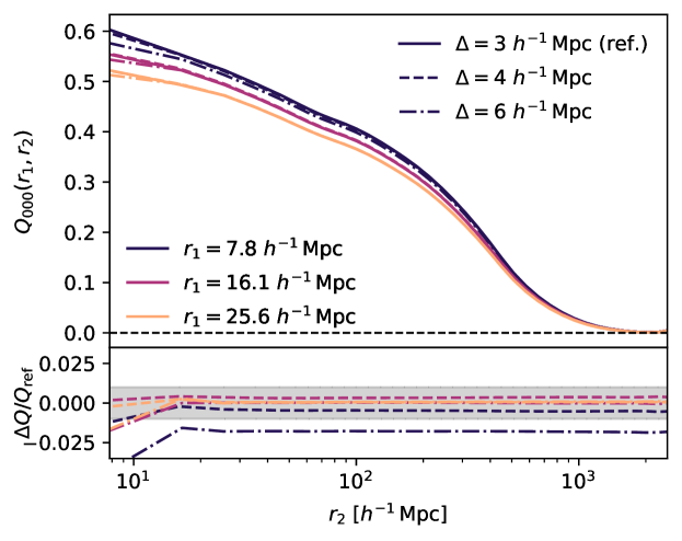
Figure 1: Three-point window function monopole $\mathop{}\!Q_{000}{\mathopen{}\mathclose{{}\left(r_{1},r_{2}}\right)}$ for the DESI DR1 LRG SGC sample in the redshift bin $$0.4$\leqslant z\leqslant$0.6$$, measured with different grid cell sizes to check convergence with respect to aliasing effects. The top panel shows the measurements at multiple small fixed values $r_{1}=$7.8$$, $16.1$ and $25.6\text{\,}{\mathrm{\text{$h$}}}^{-1}\text{\,}\mathrm{Mpc}$ with a varying mesh grid cell size $\Delta=$3$$, $4$ and $6\text{\,}{\mathrm{\text{$h$}}}^{-1}\text{\,}\mathrm{Mpc}$. The bottom panel shows the relative difference of the measurements with respect to the reference case of $\Delta=$3$\leavevmode\nobreak\ ${\mathrm{\text{$h$}}}^{-1}\text{\,}\mathrm{Mpc}$$, where the grey shaded region delimits $\pm 1\text{\,}\mathrm{\char 37\relax}$ deviations.

As the grid cell size approaches $\Delta=$3$\leavevmode\nobreak\ ${\mathrm{\text{$h$}}}^{-1}\text{\,}\mathrm{Mpc}$$, the measurement of $\mathop{}\!Q_{000}{\mathopen{}\mathclose{{}\left(r_{1},r_{2}}\right)}$ has converged to within about $1\text{\,}\mathrm{\char 37\relax}$, and hereafter this will be used as the maximum grid cell size when measuring the three-point window function.

Next, with the grid cell size fixed at $\Delta=$3$\leavevmode\nobreak\ ${\mathrm{\text{$h$}}}^{-1}\text{\,}\mathrm{Mpc}$$, we measure the diagonal window function monopole $\mathop{}\!Q_{000}{\mathopen{}\mathclose{{}\left(r,r}\right)}$ in the same separation bins for multiple mesh grid sizes $(L_{x},L_{y},L_{z})=(L,2L,L)$ where $L$ is varied.

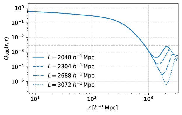
Figure 2: Diagonal three-point window function monopole $\mathop{}\!Q_{000}{\mathopen{}\mathclose{{}\left(r,r}\right)}$ for the DESI DR1 LRG SGC sample in the redshift bin $$0.4$\leqslant z\leqslant$0.6$$, measured with different mesh grid sizes to check the effect of sample variance of large-scale modes. Each line shows the measurement with a different mesh grid size $(L_{x},L_{y},L_{z})=(L,2L,L)$, where $L=$2048$$, $2304$, $2688$ and $3072\text{\,}{\mathrm{\text{$h$}}}^{-1}\text{\,}\mathrm{Mpc}$ respectively. The horizontal dashed line marks $0.5\text{\,}\mathrm{\char 37\relax}$ of the maximum value, i.e. $$0.005$\max_{r}\mathop{}\!Q_{000}{\mathopen{}\mathclose{{}\left(r,r}\right)}$.

In figure 2, we see that as $r$ increases, the window function multipole becomes vanishingly small, albeit with a nonzero fluctuating amplitude due to the sample variance of large-scale modes; however, with a greater mesh grid size, the sample variance is reduced and so is the window function residual. For the LRG SGC sample in the redshift bin $$0.4$\leqslant z\leqslant$0.6$$ considered in this section, the mesh grid size with $L=$2688\text{\,}{\mathrm{\text{$h$}}}^{-1}\text{\,}\mathrm{Mpc}$$ is adopted, as the residual amplitude of $\mathop{}\!Q_{000}{\mathopen{}\mathclose{{}\left(r,r}\right)}$ for large $r$ is suppressed to below about $0.1\text{\,}\mathrm{\char 37\relax}$ of its maximum.

4.1.2 Convergence with number density

We also test the convergence of the window function measurements with respect to the number density of the random catalogue. Typically, the number density of the random catalogue is expressed as an inverse ratio of weighted number counts compared with that of the data catalogue, $\alpha=\quantity(\sum_{\mathrm{data}}w_{\mathrm{s}})/\sum_{\mathrm{random}}w_{\mathrm{s}}$, where $w_{\mathrm{s}}$ is the systematic weight (unity if not applied).

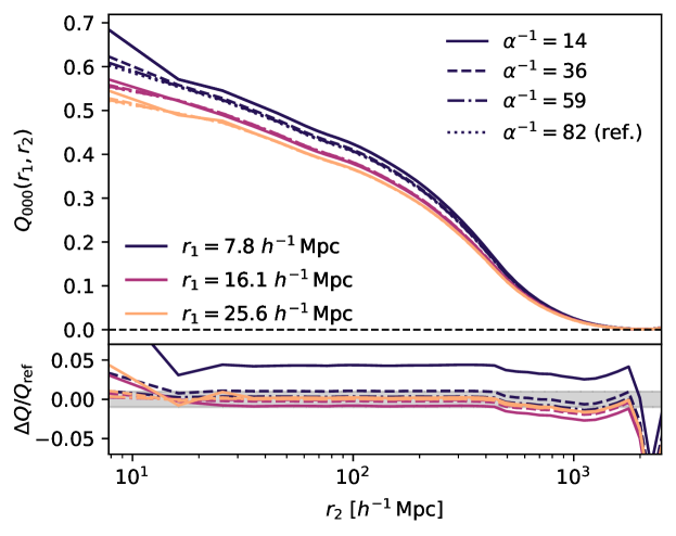
Figure 3: Three-point window function monopole $\mathop{}\!Q_{000}{\mathopen{}\mathclose{{}\left(r_{1},r_{2}}\right)}$ for the DESI DR1 LRG SGC sample in the redshift bin $$0.4$\leqslant z\leqslant$0.6$$. The top panel shows the measurements at multiple small fixed values $r_{1}=$7.8$$, $16.1$ and $25.6\text{\,}{\mathrm{\text{$h$}}}^{-1}\text{\,}\mathrm{Mpc}$ with a varying random catalogue number density ratio $\alpha^{-1}=$14$$, $36$, $59$ and $82$. The bottom panel shows the relative difference of the measurements with respect to the reference case of $\alpha^{-1}=$82$$, where the grey shaded region delimits $\pm 1\text{\,}\mathrm{\char 37\relax}$ deviations.

In figure 3, we compare the measurements at multiple small fixed values of $r_{1}$ for a varying ratio $\alpha^{-1}$. As the random catalogue becomes denser with an increasing value of $\alpha^{-1}$, the measurement of $\mathop{}\!Q_{000}{\mathopen{}\mathclose{{}\left(r_{1},r_{2}}\right)}$ has converged to within about $1\text{\,}\mathrm{\char 37\relax}$. Given that the increased number density of the random catalogue has a negligible impact on computation time, hereafter we will always use the densest random catalogue available for all measurements.

We briefly note here that the number density of the random catalogue appears to have an effect on the largest scales, but there is no discernible trend with $\alpha^{-1}$. We attribute this also to the sample variance of the large-scale modes, as the random catalogues at different number densities are fundamentally different realisations. This effect is visually more pronounced in the bottom panel of figure 3 showing the relative deviation, because the amplitude of $\mathop{}\!Q_{000}{\mathopen{}\mathclose{{}\left(r_{1},r_{2}}\right)}$ is itself small and close to zero for large $r_{2}$; the absolute deviation remains small.

Having tested the convergence of window function measurements, in figure 4 we show some of the three-point window function multipoles to be used in the convolution series in section 4.2. These measurements have been made from the densest random catalogue available ($\alpha^{-1}=$82$$) with a mesh grid of minimum dimension $L=$2688\text{\,}{\mathrm{\text{$h$}}}^{-1}\text{\,}\mathrm{Mpc}$$ and cell size $\Delta=$2.6\text{\,}{\mathrm{\text{$h$}}}^{-1}\text{\,}\mathrm{Mpc}$$.

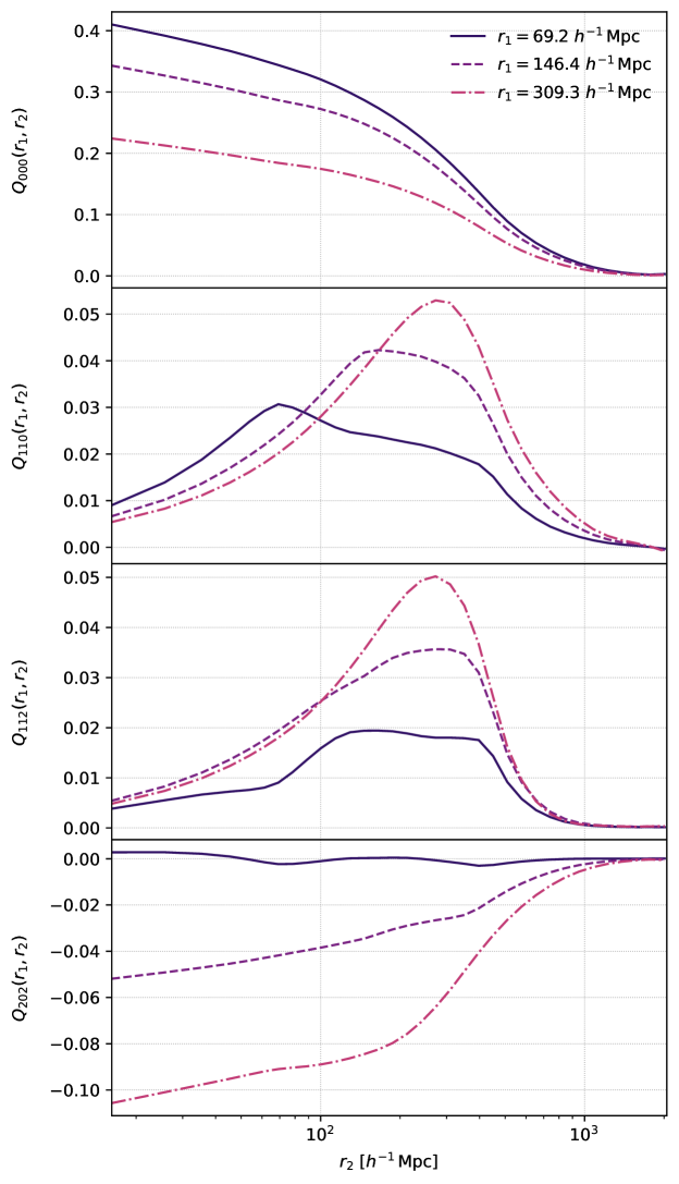
Figure 4: Some of the three-point window function multipoles $\mathop{}\!Q_{\ell_{1}\ell_{2}L}{\mathopen{}\mathclose{{}\left(r_{1},r_{2}}\right)}$ for the DESI DR1 LRG SGC sample in the redshift bin $$0.4$\leqslant z\leqslant$0.6$$, with $r_{1}$ fixed at multiple different values.

4.2 Window convolution series

In this subsection, we examine the contribution of the various terms in the window convolution series (3.5) for the bispectrum monopole $\tilde{B}_{000}$ and quadrupole $\tilde{B}_{202}$. We consider the following truncated series with a large number of 3PCF multipoles as the reference formula,

$$\tilde{\zeta}_{000} =Q_{000}\zeta_{000}$$

$$\qquad+\frac{1}{3}Q_{110}\zeta_{110}+\frac{1}{5}Q_{220}\zeta_{220}$$

$$\qquad+\frac{1}{5}\quantity(Q_{022}\zeta_{022}+Q_{202}\zeta_{202})+\frac{1}{6}Q_{112}\zeta_{112}+\frac{1}{9}\quantity(Q_{132}\zeta_{132}+Q_{312}\zeta_{312})$$

$$\qquad-Q_{000}\bar{\zeta}\,,$$ (4.1a)

$$\tilde{\zeta}_{202} =Q_{000}\zeta_{202}$$

$$\qquad+Q_{202}\zeta_{000}$$

$$\qquad+\frac{1}{3}\quantity(Q_{112}\zeta_{110}+Q_{312}\zeta_{110}+Q_{110}\zeta_{112}+Q_{110}\zeta_{312})+\frac{1}{5}\quantity(Q_{022}\zeta_{220}+Q_{220}\zeta_{022})$$

$$\qquad+\frac{2}{7}Q_{202}\zeta_{202}+\frac{1}{6}\quantity(Q_{112}\zeta_{112}+Q_{132}\zeta_{132})+\frac{8}{63}Q_{312}\zeta_{312}+\frac{1}{21}\quantity(Q_{312}\zeta_{112}+Q_{112}\zeta_{312})$$

$$\qquad-Q_{202}\bar{\zeta}\,.$$ (4.1b)

Here the set of input multipoles are $(\ell_{1},\ell_{2},L)\in\{(0,0,0),\allowbreak(1,1,0),\allowbreak(2,2,0),\allowbreak(2,0,2),\allowbreak(1,1,2),\allowbreak(1,3,2)\}$ plus their counterparts under the exchange $\ell_{1}\leftrightarrow\ell_{2}$, which include monopoles and quadrupoles with high signal-to-noise ratios. The integral constraint correction given by the series (3.6) is calculated from the same set of multipoles.

To obtain the set of unwindowed 3PCF multipoles $\mathop{}\!\zeta_{\ell_{1}\ell_{2}L}{\mathopen{}\mathclose{{}\left(r_{1},r_{2}}\right)}$, we double spherical Bessel transform the two-dimensional proxy model $\mathop{}\!B_{\ell_{1}\ell_{2}L}{\mathopen{}\mathclose{{}\left(k_{1},k_{2}}\right)}$ in $50$ logarithmic bins of wavenumber $k\in[0.001,0.520]\leavevmode\nobreak\ $\mathrm{\text{$h$}}\text{\,}{\mathrm{Mpc}}^{-1}$$ in each dimension. The window function and unwindowed 3PCF multipoles are resampled over the same logarithmically spaced points wherever necessary for the multiplication in eq. 3.5 and for the FFTLog algorithm. Finally, we double spherical Bessel transform the window-convolved 3PCF multipoles $\mathop{}\!\tilde{\zeta}_{\ell_{1}\ell_{2}L}{\mathopen{}\mathclose{{}\left(r_{1},r_{2}}\right)}$ back into Fourier space to obtain the window-convolved bispectrum multipoles $\mathop{}\!\tilde{B}_{\ell_{1}\ell_{2}L}{\mathopen{}\mathclose{{}\left(k_{1},k_{2}}\right)}$ as described in section 3.

In figure 5, we compare the window-convolved bispectrum proxy model $\tilde{B}_{\ell_{1}\ell_{2}L}$ with the windowed cut-sky measurements and the unwindowed cubic-box measurements in the wavenumber range $(0,0.12]\leavevmode\nobreak\ $\mathrm{\text{$h$}}\text{\,}{\mathrm{Mpc}}^{-1}$$.

DESI DR1 LRG SGC $$0.4$\leqslant z\leqslant$0.6$$

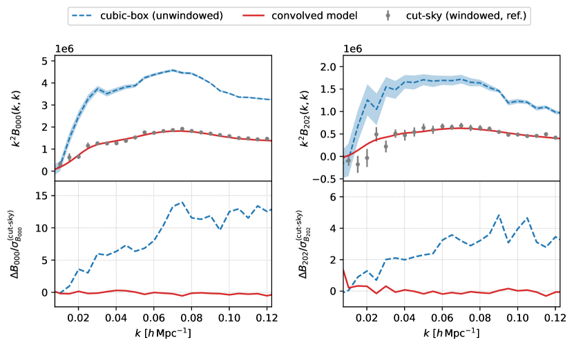
Figure 5: The top panels compare the diagonal bispectrum monopole $\mathop{}\!B_{000}{\mathopen{}\mathclose{{}\left(k,k}\right)}$ (left column) and quadrupole $\mathop{}\!B_{202}{\mathopen{}\mathclose{{}\left(k,k}\right)}$ (right column) of unwindowed cubic-box measurements, windowed cut-sky measurements and the window-convolved proxy model. The bottom panels show the deviation $\Delta{B}_{\ell_{1}\ell_{2}L}$ of the window-convolved proxy model from the cut-sky measurements as a multiple of the standard deviation $\sigma_{B_{\ell_{1}\ell_{2}L}}^{\text{(cut-sky)}}$ of the cut-sky measurements.

As mentioned earlier, we focus on the diagonal monopole and quadrupole which retain the most amount of signal relative to noise. We find that the window function significantly changes the amplitude and shape of the bispectrum multipoles; without accounting for its effect, there can be a deviation of up to $14\text{\,}\mathrm{\text{$\sigma$}}$ in the monopole $\tilde{B}_{000}$ and up to $5\text{\,}\mathrm{\text{$\sigma$}}$ in the quadrupole $\tilde{B}_{202}$, where $\sigma$ is the standard deviation of the windowed cut-sky measurements. By contrast, the window-convolved bispectrum proxy model has no noticeable deviation from the cut-sky measurements.

As a useful diagnostic tool, we consider the possibility of a constant amplitude offset of the window-convolved bispectrum proxy model from the windowed cut-sky measurements, which is parametrised as a relative difference, $\tilde{B}_{\ell_{1}\ell_{2}L}\mapsto(1+\beta)\tilde{B}_{\ell_{1}\ell_{2}L}$. To determine the amplitude offset parameter $\beta$ as well as the contribution of the various terms in the window convolution series (3.5), we define the following loss function:

$$\mathop{}\!\chi^{2}_{\ell_{1}\ell_{2}L}{\mathopen{}\mathclose{{}\left(\Lambda,\beta}\right)}=\sum_{i,j}\quantity[(1+\beta)\mathop{}\!\tilde{B}_{\ell_{1}\ell_{2}L}^{(\Lambda)}{\mathopen{}\mathclose{{}\left(k_{i},k_{i}}\right)}-\mathop{}\!B_{\ell_{1}\ell_{2}L}^{\text{(cut-sky)}}{\mathopen{}\mathclose{{}\left(k_{i},k_{i}}\right)}missing]\\ \times\quantity(\boldsymbol{\mathsf{C}}_{\ell_{1}\ell_{2}L}^{-1})_{ij}\quantity[(1+\beta)\mathop{}\!\tilde{B}_{\ell_{1}\ell_{2}L}^{(\Lambda)}{\mathopen{}\mathclose{{}\left(k_{j},k_{j}}\right)}-\mathop{}\!B_{\ell_{1}\ell_{2}L}^{\text{(cut-sky)}}{\mathopen{}\mathclose{{}\left(k_{j},k_{j}}\right)}missing]\,.$$ (4.4)

Here the diagonal window-convolved bispectrum proxy model $\mathop{}\!\tilde{B}_{\ell_{1}\ell_{2}L}^{(\Lambda)}{\mathopen{}\mathclose{{}\left(k,k}\right)}$ depends on the window convolution formula labelled by $\Lambda$, and $\boldsymbol{\mathsf{C}}_{\ell_{1}\ell_{2}L}$ is the covariance matrix of the diagonal windowed cut-sky bispectrum multipole $\mathop{}\!B_{\ell_{1}\ell_{2}L}^{\text{(cut-sky)}}{\mathopen{}\mathclose{{}\left(k,k}\right)}$ estimated from 25 measurements. These quantities are evaluated at the effective wavenumber $k_{i}$ in $12$ ($\ll 25$) bins in the range mentioned above so that the estimated covariance matrix can be inverted [68].

If we fix the window convolution formula to the reference case $\Lambda_{\mathrm{ref}}$ given by eq. 4.1, we can minimise eq. 4.4 over the amplitude offset $\beta$ to find the best-fitting value $\beta=$6\text{\times}{10}^{-3}$$ for the monopole $\tilde{B}_{000}$ and $\beta=$4\text{\times}{10}^{-2}$$ for the quadrupole $\tilde{B}_{202}$. In both cases, this value is well within the fractional error of the cubic-box measurements (which we have used as a noisy proxy model) in this scale range. We thus consider the offset to be consistent with zero and assume $\beta=0$ hereafter in this section. For the monopole $\tilde{B}_{000}$, the loss function $\chi^{2}_{000}$ is $0.08$ per wavenumber bin, and for the quadrupole $\tilde{B}_{202}$, the loss function $\chi^{2}_{202}$ is $0.03$ per wavenumber bin.

To evaluate the relative contribution of each term $Q_{\ell^{\prime\prime}_{1}\ell^{\prime\prime}_{2}L^{\prime\prime}}\zeta_{\ell^{\prime}_{1}\ell^{\prime}_{2}L^{\prime}}$ (numerical prefactor omitted in text for brevity) in eq. 4.1, we define the weight function

$$\mathop{}\!\gamma_{\ell_{1}\ell_{2}L}{\mathopen{}\mathclose{{}\left(\Lambda}\right)}={\frac{\chi^{2}_{\ell_{1}\ell_{2}L}(\Lambda,{\beta})-\chi^{2}_{\ell_{1}\ell_{2}L}(\Lambda_{\mathrm{ref}},{\beta})}{\chi^{2}_{\ell_{1}\ell_{2}L}(\Lambda_{0},{\beta})-\chi^{2}_{\ell_{1}\ell_{2}L}(\Lambda_{\mathrm{ref}},{\beta})}}\,,$$ (4.5)

where $\Lambda_{0}$ denotes the case of a zero bispectrum model, i.e. $\tilde{B}_{\ell_{1}\ell_{2}L}\equiv 0$. This weight function is akin to a sliding scale with the end-points chosen to correspond to a zero bispectrum model and the reference formula, but it should not be interpreted as a percentage contribution. We first consider a set of window function formulae $\Lambda$ each with precisely one term removed from $\Lambda_{\mathrm{ref}}$, in which case a larger value of $\mathop{}\!\gamma_{\ell_{1}\ell_{2}L}{\mathopen{}\mathclose{{}\left(\Lambda}\right)}$ indicates a more significant term, since its removal leads to a greater deviation in the window-convolved bispectrum model. In figure 6, we show the absolute weight function value of the various terms in the reference window convolution formula (4.1) for the bispectrum monopole $\tilde{B}_{000}$ and quadrupole $\tilde{B}_{202}$ separately.

DESI DR1 LRG SGC $$0.4$\leqslant z\leqslant$0.6$$

Figure 6: Absolute values of the weight function (4.5), $100\absolutevalue{\mathop{}\!\gamma_{\ell_{1}\ell_{2}L}{\mathopen{}\mathclose{{}\left(\Lambda}\right)}missing}$, for each convolution formula $\Lambda$ with precisely one term $Q_{\ell^{\prime\prime}_{1}\ell^{\prime\prime}_{2}L^{\prime\prime}}\zeta_{\ell^{\prime}_{1}\ell^{\prime}_{2}L^{\prime}}$ removed from the reference formula $\Lambda_{\mathrm{ref}}$ given by eq. 4.1. For visual clarity, the values have been multiplied by 100 and the colour map is in a logarithmic scale. Sub-figure (LABEL:fig:window-contribution-remove-monopole) shows the relative contribution of each term to the windowed bispectrum monopole $\tilde{B}_{000}$, and sub-figure (LABEL:fig:window-contribution-remove-quadrupole) to the windowed quadrupole $\tilde{B}_{202}$.

It is clear that the latter terms in the reference formula (4.1), e.g. those with the multipole factor $\zeta_{132}$ or $\zeta_{312}$, are negligible. The integral constraint correction is also negligible for both the monopole $\tilde{B}_{000}$ and the quadrupole $\tilde{B}_{202}$.

To visualise the convergence of the window convolution series, in figure 7 we consider the quantity $(1-\gamma_{\ell_{1}\ell_{2}L})$ for a set of window function formulae $\Lambda$ that cumulatively adds each term in eq. 4.1, starting from the leading term, i.e. $\tilde{\zeta}_{\ell_{1}\ell_{2}L}=Q_{000}\zeta_{\ell_{1}\ell_{2}L}$. Once sufficiently many terms have been included, the value of $(1-\gamma_{\ell_{1}\ell_{2}L})$ should stabilise to $1$, as observed in figure 7.

DESI DR1 LRG SGC $$0.4$\leqslant z\leqslant$0.6$$

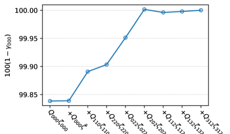
(a) monopole $\tilde{B}_{000}$ convergence

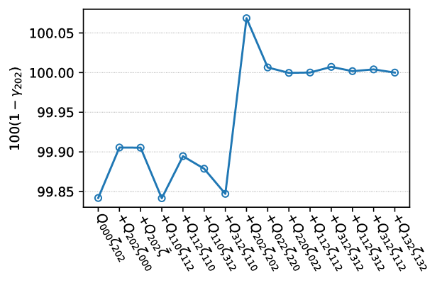
(b) quadrupole $\tilde{B}_{202}$ convergence

Figure 7: The quantity $100(1-{\gamma_{\ell_{1}\ell_{2}L}})$, where $\mathop{}\!\gamma_{\ell_{1}\ell_{2}L}{\mathopen{}\mathclose{{}\left(\Lambda}\right)}$ is the weight function (4.5), for a series of convolution formulae $\Lambda$ that adds each term $Q_{\ell^{\prime\prime}_{1}\ell^{\prime\prime}_{2}L^{\prime\prime}}\zeta_{\ell^{\prime}_{1}\ell^{\prime}_{2}L^{\prime}}$ cumulatively to the leading term $Q_{000}\zeta_{\ell_{1}\ell_{2}L}$. Sub-figure (7(a)) shows the convergence of the window convolution formula (4.1) for the windowed bispectrum monopole $\tilde{B}_{000}$, and sub-figure (7(b)) for the windowed quadrupole $\tilde{B}_{202}$.

Based on figures 6 and 7, we can write down a window convolution formula from a reduced set of multipoles by removing terms with $\absolutevalue{\gamma_{000}},\absolutevalue{\gamma_{202}}<{$4\text{\times}{10}^{-4}$}$,

$$\tilde{\zeta}_{000} =Q_{000}\zeta_{000}+\frac{1}{3}Q_{110}\zeta_{110}+\frac{1}{5}\quantity(Q_{022}\zeta_{022}+Q_{202}\zeta_{202})\,,$$ (4.6a)

$$\tilde{\zeta}_{202} =Q_{000}\zeta_{202}+Q_{202}\zeta_{000}+\frac{1}{3}\quantity(Q_{112}\zeta_{110}+Q_{110}\zeta_{112})+{\frac{1}{5}Q_{022}\zeta_{220}}+\frac{2}{7}Q_{202}\zeta_{202}\,.$$ (4.6b)

The loss function (4.4) remains the same as for the full reference formula, at $0.08$ for the monopole $\tilde{B}_{000}$ and $0.03$ for the quadrupole $\tilde{B}_{202}$ per wavenumber bin. In the next subsection, we will use this reduced window convolution formula to test the window matrix in the linear algebra formulation.

Although the validation tests in this section have focused on the LRG SGC sample in the redshift bin $$0.4$\leqslant z\leqslant$0.6$$ in DESI DR1, we have also checked other samples such as quasars (QSO) in the North Galactic Cap (NGC) in the redshift range $0.8\leqslant z\leqslant 2.1$. These results are presented in appendix A.

4.3 Window matrix performance

When the set of unwindowed model multipoles $\zeta_{\ell_{1}\ell_{2}L}$ included in the window convolution formula for different windowed model multipoles $\tilde{\zeta}_{\ell_{1}\ell_{2}L}$ do not entirely coincide, the overall window matrix $\boldsymbol{\mathsf{W}}$ will contain sparse sub-matrices. In such cases, it may be computationally advantageous to consider the window matrix for each required windowed multipole separately. Without loss of generality, we compute in this subsection the window matrices for the bispectrum monopole $\tilde{B}_{000}$ and quadrupole $\tilde{B}_{202}$ separately, which correspond to the two reduced window convolution formulae (4.6).

The input bispectrum multipoles $\mathop{}\!B_{\ell_{1}\ell_{2}L}{\mathopen{}\mathclose{{}\left(k_{1},k_{2}}\right)}$ are as before the proxy model obtained from the mean of the cubic-box measurements, which have been resampled from $50$ to $$64$=2^{6}$ logarithmic bins in $k_{1,2}$. We fix the ordering of the multipoles as they appear in eq. 4.6 to form the vectorised bispectrum model vector $\mathbf{B}$. To generate the window matrix $\boldsymbol{\mathsf{W}}$, we feed a basis of unit vectors as $\mathbf{B}$ into the full window convolution recipe as described in section 3.3. This results in window matrices of dimensions $(64^{2},4\times 64^{2})$ for the monopole $\tilde{B}_{000}$ and $(64^{2},5\times 64^{2})$ for the quadrupole $\tilde{B}_{202}$, since the input bispectrum multipoles are two-dimensional before vectorisation and there are respectively four and five unwindowed model multipoles required by them in eq. 4.6. Although the sub-matrices of $\boldsymbol{\mathsf{W}}$ here are square with dimensions $(64^{2},64^{2})$ as the numbers of input and output FFTLog sample points are the same, generally they can be non-square with more columns (input sample points) than rows (output sample points); to compare with the windowed cut-sky bispectrum data vector with fewer wavenumber bins, a simple interpolation step can be performed after convolution. In figure 8, we show the structure of the window matrices $\boldsymbol{\mathsf{W}}$ for the windowed bispectrum monopole $\tilde{B}_{000}$ and quadrupole $\tilde{B}_{202}$.

DESI DR1 LRG SGC $$0.4$\leqslant z\leqslant$0.6$$

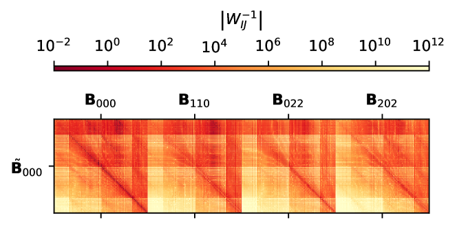
(a) window matrix for monopole $\tilde{B}_{000}$

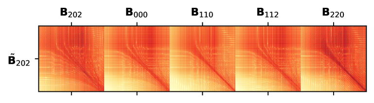
(b) window matrix for quadrupole $\tilde{B}_{202}$

Figure 8: Inverse absolute value of the window matrix elements, $\quantity(\boldsymbol{\mathsf{W}})_{IJ}^{-1}$, for the windowed bispectrum monopole $\tilde{B}_{000}$ (sub-figure 8(a)) and quadrupole $\tilde{B}_{202}$ (sub-figure 8(b)) according to the reduced window convolution formula (4.6). The column blocks of the matrix corresponds to the input unwindowed bispectrum multipole vectors $\mathbf{B}_{\ell_{1}\ell_{2}L}$, and the rows corresponds to the output windowed bispectrum multipole vectors $\tilde{\mathbf{B}}_{{\ell_{1}\ell_{2}L}}$.

Whether we compute the windowed bispectrum multipole from the window matrix multiplication $\tilde{\mathbf{B}}=\boldsymbol{\mathsf{W}}\mathbf{B}$ or following the step-by-step recipe in section 3.3, the results are found to agree within floating-point arithmetic precision. However, the full convolution pipeline without using the window matrix takes order ${10}^{-1}\text{\,}\mathrm{s}$ on a single processor core, whereas the window matrix multiplication takes order ${10}^{-2}\text{\,}\mathrm{s}$. While the initial computation of the window matrix can be relatively expensive, it can be easily parallelised and only needs to be done once, as long as the wavenumber sample points remain the same; by contrast, window convolution needs to be performed repeatedly in a cosmological inference analysis. Finally, in figure 12 in appendix B, we show the matrix multiplication time for a range of matrix dimensions similar to the window matrix considered in this section. We note that the execution time is all below ${10}^{-1}\text{\,}\mathrm{s}$, and thus the linear algebra formulation of window convolution will be performant and well-suited for cosmological likelihood analyses.

5 Conclusion

Window convolution for the galaxy clustering bispectrum has long been a challenging issue: its formulation is usually analytically complex, and the window function itself is computationally expensive to estimate. The problem stems from the so-called ‘curse of dimensionality’, as the 3PCF or bispectrum in Fourier space has more degrees of freedom than the two-point correction function (2PCF) and the power spectrum. With the advent of Stage IV spectroscopic surveys including DESI and Euclid, non-Gaussian clustering statistics have become a frontier in driving the exploration of cosmological models; as such, the survey window effect which modulates both the amplitude and shape of the three-point clustering statistics must be properly accounted for through forward modelling.

We have built on the TripoSH formalism developed in refs. [32, 33] to address some of these difficulties. In this decomposition, the bispectrum multipoles in redshift space are functions of two wavenumbers instead of a full triangle configuration, thus providing a natural form of data reduction and avoiding the triangle binning issue. At the same time, the window convolution series derived in this formalism are structurally similar to that of the 2PCF/power spectrum [12, 13, 15], and require window function multipoles that can be conveniently estimated using FFTs in the same way as for the 3PCF. In particular, by utilising the linear algebra nature of the window convolution operations, we have proposed a formulation that encapsulates the full procedure as a window matrix multiplication.

In this work, we have focused on tracer samples in the DESI DR1 data release, and employed a suite of unwindowed cubic-box snapshots and windowed cut-sky catalogues with the same underlying clustering signal, to validate the window convolution pipeline for the bispectrum. We have checked the convergence of the window function measurements with respect to FFT sampling and the number density of the random catalogue, and highlighted some of the technicalities that differ from the case of the two-point window function. We have also systematically verified the convergence of the window convolution series truncated at a finite but large number of terms, which has been either ignored or performed in configuration space for 3PCF in previous works [32, 33]. The window matrix formulation is found to provide the same results as the full convolution procedure, but with a computation time that is an order of magnitude lower once it has been generated.

The results in this work offer a replicable window convolution pipeline to implement for generic survey configurations, with all the computational tools publicly available as part of the Triumvirate code (see footnote 2 or Data Availability for the link). However, we caution that the convergence of the window function measurements and the window convolution series depends on the specific survey geometry and scales of interest, and should be verified in each case as detailed in section 4.

Finally, some topics remain to be explored, such as the performance of alternative algorithms for the double spherical Bessel transform and the scale-dependent integral constraint, including the radial integral constraint. We leave these issues for future studies.

Data Availability

The data underlying this article will be made public along with DESI DR1 (see data.desi.lbl.gov/doc for details) as part of the DESI Data Management Plan.

The source code used to process and generate the relevant data in this article is made freely available under the GPLv3+ licence in the GitHub repository at github.com/MikeSWang/Triumvirate.

Appendix A Window convolution tests of additional samples

We have additionally studied the DESI DR1 QSO sample which has a single redshift bin $0.8\leqslant z\leqslant 2.1$ in both NGC and SGC, and is lower in number density and higher in redshift compared to the LRG sample studied in section 4. For the NGC sample which has a larger survey footprint, we measure the window function multipoles ${Q_{\ell_{1}\ell_{2}L}}$ using a random catalogue $\alpha^{-1}\approx 127$ times denser than the data catalogue with a mesh grid of minimum dimension $L=$8000\text{\,}{\mathrm{\text{$h$}}}^{-1}\text{\,}\mathrm{Mpc}$$ and cell size $\Delta=$7.8\text{\,}{\mathrm{\text{$h$}}}^{-1}\text{\,}\mathrm{Mpc}$$, which is limited by the computational memory available. Both data and random mock catalogues have been generated from the ATMLs which simulate fibre assignment in DESI observations.

Starting from the same reference formula (4.1) and the weight function (4.5) in section 4.2, we derive the convergent window convolution series based on the criterion $\absolutevalue{\gamma_{\ell_{1}\ell_{2}L}}\geqslant$5\text{\times}{10}^{-4}$$,

$$\tilde{\zeta}_{000} =Q_{000}\zeta_{000}+\frac{1}{3}Q_{110}\zeta_{110}+\frac{1}{5}Q_{220}\zeta_{220}-Q_{000}\bar{\zeta}\,,$$ (A.1a)

$$\tilde{\zeta}_{202} =Q_{000}\zeta_{202}+Q_{202}\zeta_{000}+\frac{1}{3}\quantity(Q_{112}\zeta_{110}+Q_{110}\zeta_{312}+Q_{312}\zeta_{110})$$

$$\qquad+\frac{1}{5}Q_{022}\zeta_{220}+\frac{2}{7}Q_{202}\zeta_{202}-Q_{202}\bar{\zeta}\,.$$ (A.1b)

In figure 9, we compare the window-convolved bispectrum proxy model $\tilde{B}_{\ell_{1}\ell_{2}L}$ with the windowed cut-sky measurements and the unwindowed cubic-box measurements in the wavenumber range $(0,0.12]\leavevmode\nobreak\ $\mathrm{\text{$h$}}\text{\,}{\mathrm{Mpc}}^{-1}$$.

DESI DR1 QSO NGC $$0.8$\leqslant z\leqslant$2.1$$

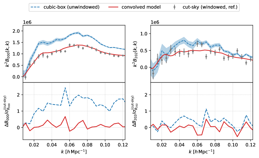
Figure 9: The same as figure 5 but for the DESI DR1 QSO NGC sample in the redshift bin $$0.8$\leqslant z\leqslant$2.1$$.

As before, the effect of the window function is significant especially for the bispectrum monopole $\tilde{B}_{000}$, but to a lesser extent than the LRG SGC sample as the larger survey volume reduces the impact of the window function in this scale range. The window-convolved model matches the amplitude and shape of the cut-sky measurements well, with the loss function $\chi^{2}_{\ell_{1}\ell_{2}L}$ (eq. 4.4) per wavenumber bin valued at $0.03$ for the monopole $\tilde{B}_{000}$ and $0.12$ for the quadrupole $\tilde{B}_{202}$. If we allow for a relative amplitude offset $\beta$ and minimise eq. 4.4 over it, we find $\beta$ consistent with zero offset for both the monopole $\tilde{B}_{000}$ and quadrupole $\tilde{B}_{202}$ within the fractional error of the cubic-box measurements used as the noisy proxy model.

However, when we test the window convolution pipeline on complete LRG mock catalogues without fibre assignment (in the SGC redshift bin $$0.4$\leqslant z\leqslant$0.6$$), we find there is a small and almost constant amplitude offset. The convergent window convolution series satisfying $\absolutevalue{\gamma_{\ell_{1}\ell_{2}L}}\geqslant$5\text{\times}{10}^{-4}$$ are given by

$$\tilde{\zeta}_{000} =Q_{000}\zeta_{000}+\frac{1}{3}Q_{110}\zeta_{110}+\frac{1}{5}\quantity(Q_{022}\zeta_{022}+Q_{220}\zeta_{220})-Q_{000}\bar{\zeta}\,,$$ (A.2a)

$$\tilde{\zeta}_{202} =Q_{000}\zeta_{202}+Q_{202}\zeta_{000}+\frac{1}{3}\quantity(Q_{112}\zeta_{110}+Q_{110}\zeta_{112})+\frac{2}{7}Q_{202}\zeta_{202}-Q_{202}\bar{\zeta}\,.$$ (A.2b)

When the loss function $\chi^{2}_{\ell_{1}\ell_{2}L}$ is minimised over $\beta$, we find $\beta=$9\text{\times}{10}^{-2}$$ for the monopole $\tilde{B}_{000}$ and quadrupole $\tilde{B}_{202}$. In figure 10, we make the same comparison as before between windowed and unwindowed bispectrum multipoles including the window-convolved model rescaled by $(1+\beta)$ to account for the amplitude offset.

DESI DR1 LRG SGC $$0.4$\leqslant z\leqslant$0.6$$ (complete mock catalogues)

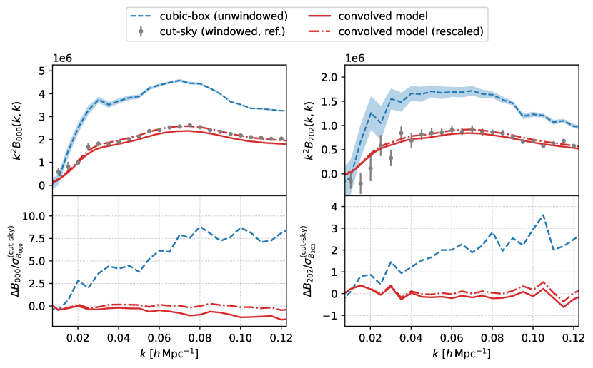
Figure 10: The same as figure 5 but for the complete mock catalogues. In addition, the window-convolved proxy model rescaled by $(1+\beta)$ is shown where $\beta=$9\text{\times}{10}^{-2}$$ accounts for the amplitude offset.

With this amplitude rescaling, the loss function value per wavenumber bin reduces from $0.62$ to $0.28$ for the monopole $\tilde{B}_{000}$ and $0.11$ to $0.07$ for the quadrupole $\tilde{B}_{202}$. We have checked that the optimal value of $\beta$ does not change significantly with the measurement parameters of the window function multipoles such as the mesh grid physical size, cell resolution and the random catalogue number density, or when the full reference formula is used.

We have repeated the same checks with the complete QSO mock catalogues in both NGC and SGC in the redshift bin $$0.8$\leqslant z\leqslant$2.1$$, but do not find any significant amplitude offset (see LABEL:{fig:window-convolution-reduced-add-QSO-NGC-complete} for the NGC case).

DESI DR1 QSO NGC $$0.8$\leqslant z\leqslant$2.1$$ (complete mock catalogues)

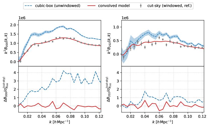
Figure 11: The same as figure 9 but for the complete mock catalogues.

We thus suspect there may be systematic effects specific to the complete LRG mock catalogues; the relative amplitude offset parameter $\beta$, as well as being a diagnostic tool in conjunction with the loss function $\chi^{2}_{\ell_{1}\ell_{2}L}$, also serves as a useful nuisance parameter to absorb unknown systematic residuals in window convolution. In the cosmological analysis of DESI DR1 samples, it is the AMTL not complete mock catalogues that will be used to validate the full pipeline as they resemble the actual survey data more closely; therefore, the validation of our window convolution pipeline with the AMTL mock catalogues in this work is more important.

Appendix B Window matrix multiplication computation time

We consider a range of window matrix dimensions $(Nd,4Nd)$, where $d=1024$ is the base dimension and $N\in\quantity{2,4,8,12,16}$ is an integer multiplier. For instance, the window matrix $\boldsymbol{\mathsf{W}}$ for the windowed bispectrum monopole $\tilde{B}_{000}$ used in section 4.2 has $N=4$. In figure 12, we plot the measured processor time of matrix multiplication for random matrices generated with these dimensions and compare three matrix multiplication methods available in the public NumPy Python package [69]. These multiplication methods perform similarly well, with an execution time all below ${10}^{-1}\text{\,}\mathrm{s}$; therefore, the window matrix multiplication step will not be the dominant operation in a typical cosmological likelihood analysis.

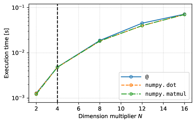
Figure 12: Matrix multiplication time for a range of possible dimensions $(Nd,4Nd)$ for the window matrix $\boldsymbol{\mathsf{W}}$, measured for three matrix multiplication methods available in the public NumPy Python package. Here $d=1024$ is the base dimension considered, and $N$ is an integer multiplier. The dashed vertical line at $N=4$ marks the (row) dimension of the window matrix $\boldsymbol{\mathsf{W}}$ used for the windowed bispectrum monopole $\tilde{B}_{000}$ in section 4.2.

References

- [1] H.A. Feldman, N. Kaiser and J.A. Peacock, Power-Spectrum Analysis of Three-dimensional Redshift Surveys, Astrophys. J. 426 (1994) 23 [astro-ph/9304022].
- [2] J.A. Peacock and D. Nicholson, The large-scale clustering of radio galaxies, Mon. Not. Roy. Astron. Soc. 253 (1991) 307.
- [3] A.J.S. Hamilton, Linear Redshift Distortions: A Review, in The Evolving Universe, D. Hamilton, ed., pp. 185–275, Kluwer Academic (1998), doi:10.1007/978-94-011-4960-0_17 [astro-ph/9708102].
- [4] F. Beutler, S. Saito, H.-J. Seo, J. Brinkmann, K.S. Dawson, D.J. Eisenstein et al., The clustering of galaxies in the SDSS-III Baryon Oscillation Spectroscopic Survey: testing gravity with redshift space distortions using the power spectrum multipoles, Mon. Not. Roy. Astron. Soc. 443 (2014) 1065 [1312.4611].
- [5] M. Tegmark, How to measure CMB power spectra without losing information, Phys. Rev. 55 (1997) 5895 [astro-ph/9611174].
- [6] M. Tegmark, A.N. Taylor and A.F. Heavens, Karhunen-Loève Eigenvalue Problems in Cosmology: How Should We Tackle Large Data Sets?, Astrophys. J. 480 (1997) 22 [astro-ph/9603021].
- [7] A.J.S. Hamilton, Towards optimal measurement of power spectra - I. Minimum variance pair weighting and the Fisher matrix, Mon. Not. Roy. Astron. Soc. 289 (1997) 285–294 [astro-ph/9701008].
- [8] A.J.S. Hamilton, Towards optimal measurement of power spectra - II. A basis of positive, compact, statistically orthogonal kernels, Mon. Not. Roy. Astron. Soc. 289 (1997) 295–304 [astro-ph/9701009].
- [9] M. Tegmark, A.J.S. Hamilton, M.A. Strauss, M.S. Vogeley and A.S. Szalay, Measuring the Galaxy Power Spectrum with Future Redshift Surveys, Astrophys. J. 499 (1998) 555 [astro-ph/9708020].
- [10] O.H.E. Philcox, Cosmology without window functions: Quadratic estimators for the galaxy power spectrum, Phys. Rev. 103 (2021) 103504 [2012.09389].
- [11] O.H.E. Philcox, Cosmology without window functions. II. Cubic estimators for the galaxy bispectrum, Phys. Rev. 104 (2021) 123529 [2107.06287].
- [12] M.J. Wilson, J.A. Peacock, A.N. Taylor and S. de la Torre, Rapid modelling of the redshift-space power spectrum multipoles for a masked density field, Mon. Not. Roy. Astron. Soc. 464 (2016) 3121–3130 [1511.07799].
- [13] F. Beutler, H.-J. Seo, S. Saito, C.-H. Chuang, A.J. Cuesta, D.J. Eisenstein et al., The clustering of galaxies in the completed SDSS-III Baryon Oscillation Spectroscopic Survey: anisotropic galaxy clustering in Fourier space, Mon. Not. Roy. Astron. Soc. 466 (2016) 2242 [1607.03150].
- [14] C. Blake, P. Carter and J. Koda, Power spectrum multipoles on the curved sky: an application to the 6-degree Field Galaxy Survey, Mon. Not. Roy. Astron. Soc. 479 (2018) 5168–5183 [1801.04969].
- [15] F. Beutler and P. McDonald, Unified galaxy power spectrum measurements from 6dFGS, BOSS, and eBOSS, JCAP 2021 (2021) 031 [2106.06324].
- [16] F. Beutler, H.-J. Seo, A.J. Ross, P. McDonald, S. Saito, A.S. Bolton et al., The clustering of galaxies in the completed SDSS-III Baryon Oscillation Spectroscopic Survey: baryon acoustic oscillations in the Fourier space, Mon. Not. Roy. Astron. Soc. 464 (2017) 3409 [1607.03149].
- [17] H. Gil-Marín, J.E. Bautista, R. Paviot, M. Vargas-Magaña, S. de la Torre, S. Fromenteau et al., The completed SDSS-IV extended Baryon Oscillation Spectroscopic Survey: measurement of the BAO and growth rate of structure of the luminous red galaxy sample from the anisotropic power spectrum between redshifts and , Mon. Not. Roy. Astron. Soc. 498 (2020) 2492 [2007.08994].
- [18] A. de Mattia, V. Ruhlmann-Kleider, A. Raichoor, A.J. Ross, A. Tamone, C. Zhao et al., The completed SDSS-IV extended Baryon Oscillation Spectroscopic Survey: measurement of the BAO and growth rate of structure of the emission line galaxy sample from the anisotropic power spectrum between redshift and , Mon. Not. Roy. Astron. Soc. 501 (2021) 5616 [2007.09008].
- [19] R. Neveux, E. Burtin, A. de Mattia, A. Smith, A.J. Ross, J. Hou et al., The Completed SDSS-IV extended Baryon Oscillation Spectroscopic Survey: BAO and RSD measurements from the anisotropic power spectrum of the quasar sample between redshift and , Mon. Not. Roy. Astron. Soc. 499 (2020) 210 [2007.08999].
- [20] D. Baumann, A. Nicolis, L. Senatore and M. Zaldarriaga, Cosmological non-linearities as an effective fluid, JCAP (2012) 051 [1004.2488].
- [21] J.J.M. Carrasco, M.P. Hertzberg and L. Senatore, The effective field theory of cosmological large scale structures, J. High Energy Phys. 2012 (2012) 082 [1206.2926].
- [22] M.P. Hertzberg, Effective field theory of dark matter and structure formation: Semianalytical results, Phys. Rev. 89 (2014) 043521 [1208.0839].
- [23] L. Senatore and M. Zaldarriaga, The IR-resummed Effective Field Theory of Large Scale Structures, JCAP 2015 (2015) 013 [1404.5954].
- [24] L. Senatore, Bias in the effective field theory of large scale structures, JCAP 2015 (2015) 007 [1406.7843].
- [25] G. d’Amico, J. Gleyzes, N. Kokron, K. Markovic, L. Senatore, P. Zhang et al., The cosmological analysis of the SDSS/BOSS data from the Effective Field Theory of Large-Scale Structure, JCAP 2020 (2020) 005 [1909.05271].
- [26] M.M. Ivanov, M. Simonovic̀ and M. Zaldarriaga, Cosmological parameters from the BOSS galaxy power spectrum, JCAP 2020 (2020) 042 [1909.05277].
- [27] H. Gil-Marín, J. Noreña, L. Verde, W.J. Percival, C. Wagner, M. Manera et al., The power spectrum and bispectrum of SDSS DR11 BOSS galaxies –- I. Bias and gravity, Mon. Not. Roy. Astron. Soc. 451 (2015) 539–580 [1407.5668].
- [28] H. Gil-Marín, W.J. Percival, L. Verde, J.R. Brownstein, C.-H. Chuang, F.-S. Kitaura et al., The clustering of galaxies in the SDSS-III Baryon Oscillation Spectroscopic Survey: RSD measurement from the power spectrum and bispectrum of the DR12 BOSS galaxies, Mon. Not. Roy. Astron. Soc. 465 (2016) 1757–1788 [1606.00439].
- [29] D. Alkhanishvili, C. Porciani and E. Sefusatti, Window function convolution with deep neural network models, Astron. Astrophys. 669 (2023) L2 [2212.09742].
- [30] R. Scoccimarro, Fast estimators for redshift-space clustering, Phys. Rev. 92 (2015) 083532 [1506.02729].
- [31] K. Pardede, F. Rizzo, M. Biagetti, E. Castorina, E. Sefusatti and P. Monaco, Bispectrum-window convolution via hankel transform, JCAP 2022 (2022) 066 [2203.04174].
- [32] N.S. Sugiyama, S. Saito, F. Beutler and H.-J. Seo, A complete FFT-based decomposition formalism for the redshift-space bispectrum, Mon. Not. Roy. Astron. Soc. 484 (2019) 364 [1803.02132].
- [33] N.S. Sugiyama, S. Saito, F. Beutler and H.-J. Seo, Towards a self-consistent analysis of the anisotropic galaxy two- and three-point correlation functions on large scales: application to mock galaxy catalogues, Mon. Not. Roy. Astron. Soc. 501 (2020) 2862–2896 [2010.06179].
- [34] M.S. Wang, F. Beutler and N.S. Sugiyama, Triumvirate: A Python/C++ package for three-point clustering measurements, J. Open Source Softw. 8 (2023) 5571 [2304.03643].
- [35] K. Yamamoto, M. Nakamichi, A. Kamino, B.A. Bassett and H. Nishioka, A Measurement of the Quadrupole Power Spectrum in the Clustering of the 2dF QSO Survey, Pub. Astron. Soc. Jap. 58 (2006) 93 [astro-ph/0505115].
- [36] Y.P. Jing, Correcting for the Alias Effect When Measuring the Power Spectrum Using a Fast Fourier Transform, Astrophys. J. 620 (2005) 559 [astro-ph/0409240].
- [37] E. Sefusatti, M. Crocce, R. Scoccimarro and H.M.P. Couchman, Accurate estimators of correlation functions in Fourier space, Mon. Not. Roy. Astron. Soc. 460 (2016) 3624 [1512.07295].
- [38] A. de Mattia and V. Ruhlmann-Kleider, Integral constraints in spectroscopic surveys, JCAP 2019 (2019) 036 [1904.08851].
- [39] J.D. Talman, Numerical Fourier and Bessel Transforms in Logarithmic Variables, J. Comput. Phys. 29 (1978) 35.
- [40] A.J.S. Hamilton, Uncorrelated modes of the non-linear power spectrum, Mon. Not. Roy. Astron. Soc. 312 (2000) 257 [astro-ph/9905191].
- [41] M. Karamanis and F. Beutler, “hankl: Python implementation of the FFTLog algorithm for cosmology.” Astrophysics Source Code Library, record ascl:2112.022, 2021.
- [42] X. Fang, T. Eifler and E. Krause, 2D-FFTLog: efficient computation of real-space covariance matrices for galaxy clustering and weak lensing, Mon. Not. Roy. Astron. Soc. 497 (2020) 2699–2714 [2004.04833].
- [43] D. Levin, Fast integration of rapidly oscillatory functions, J. Comput. Appl. Math. 67 (1996) 95.
- [44] D. Levin, Analysis of a collocation method for integrating rapidly oscillatory functions, J. Comput. Appl. Math. 78 (1997) 131.
- [45] C.D. Leonard, T. Ferreira, X. Fang, R. Reischke, N. Schoeneberg, T. Tröster et al., The N5K Challenge: Non-Limber Integration for LSST Cosmology, Open J. Astrophys. 6 (2023) [2212.04291].
- [46] J. Feldbrugge, Complex evaluation of angular power spectra: Going beyond the Limber approximation, Phys. Rev. 108 (2023) 103007 [2304.13064].
- [47] M. Levi, C. Bebek, T. Beers, R. Blum, R. Cahn, D. Eisenstein et al., The DESI Experiment, a whitepaper for Snowmass 2013, preprint (2013) [1308.0847].
- [48] DESI Collaboration, The DESI Experiment Part I: Science,Targeting, and Survey Design, preprint (2016) [1611.00036].
- [49] DESI Collaboration, The DESI Experiment Part II: Instrument Design, preprint (2016) [1611.00037].
- [50] DESI Collaboration, Overview of the Instrumentation for the Dark Energy Spectroscopic Instrument, Astron. J. 164 (2022) 207 [2205.10939].
- [51] DESI Collaboration, Validation of the Scientific Program for the Dark Energy Spectroscopic Instrument, Astron. J. 167 (2024) 62 [2306.06307].
- [52] DESI Collaboration, The Early Data Release of the Dark Energy Spectroscopic Instrument, Astron. J. 168 (2024) 58 [2306.06308].
- [53] DESI Collaboration, DESI 2024 I: Data Release 1 of the Dark Energy Spectroscopic Instrument, in preparation (2024) .
- [54] DESI Collaboration, DESI 2024 II: Sample definitions, characteristics and two-point clustering statistics, in preparation (2024) .
- [55] DESI Collaboration, DESI 2024 III: Baryon Acoustic Oscillations from Galaxies and Quasars, preprint (2024) [2404.03000].
- [56] DESI Collaboration, DESI 2024 IV: Baryon Acoustic Oscillations from the Lyman Alpha Forest, preprint (2024) [2404.03001].
- [57] DESI Collaboration, DESI 2024 VI: Cosmological Constraints from the Measurements of Baryon Acoustic Oscillations, preprint (2024) [2404.03002].
- [58] J.H. Silber, P. Fagrelius, K. Fanning, M. Schubnell, J.N. Aguilar, S. Ahlen et al., The Robotic Multiobject Focal Plane System of the Dark Energy Spectroscopic Instrument (DESI), Astron. J. 165 (2023) 9 [2205.10939].
- [59] T.N. Miller, P. Doel, G. Gutierrez, R. Besuner, Brooks et al., The Optical Corrector for the Dark Energy Spectroscopic Instrument, Astron. J. 168 (2023) 95 [2306.06310].
- [60] J. Guy, S. Bailey, A. Kremin, S. Alam, D.M. Alexander, C. Allende Prieto et al., The Spectroscopic Data Processing Pipeline for the Dark Energy Spectroscopic Instrument, Astron. J. 165 (2023) 144 [2209.14482].
- [61] E.F. Schlafly, D. Kirkby, D.J. Schlegel, A.D. Myers, A. Raichoor, K. Dawson et al., Survey Operations for the Dark Energy Spectroscopic Instrument, Astron. J. 166 (2023) 259 [2306.06309].
- [62] R. Zhou, B. Dey, J.A. Newman, D.J. Eisenstein, K. Dawson, S. Bailey et al., Target Selection and Validation of DESI Luminous Red Galaxies, Astron. J. 165 (2023) 58 [2208.08515].
- [63] N.A. Maksimova, L.H. Garrison, D.J. Eisenstein, B. Hadzhiyska, S. Bose and T.P. Satterthwaite, AbacusSummit: a massive set of high-accuracy, high-resolution N-body simulations, Mon. Not. Roy. Astron. Soc. 508 (2021) 4017 [2110.11398].
- [64] L.H. Garrison, D.J. Eisenstein, D. Ferrer, N.A. Maksimova and P.A. Pinto, The abacus cosmological N-body code, Mon. Not. Roy. Astron. Soc. 508 (2021) 575 [2110.11392].
- [65] Planck Collaboration, Planck 2018 results. VI. Cosmological parameters, Astron. Astrophys. 641 (2020) A6 [1807.06209].
- [66] S. Yuan, H. Zhang, A.J. Ross, J. Donald-McCann, B. Hadzhiyska, R.H. Wechsler et al., The DESI one-per cent survey: exploring the halo occupation distribution of luminous red galaxies and quasi-stellar objects with AbacusSummit, Mon. Not. Roy. Astron. Soc. 530 (2024) 947 [2306.06314].
- [67] J. Lasker, A.C. Rosell, A.D. Myers, A.J. Ross, D. Bianchi, M.M.S. Hanif et al., Production of Alternate Realizations of DESI Fiber Assignment for Unbiased Clustering Measurement in Data and Simulations, preprint (2024) [2404.03006].
- [68] J. Hartlap, P. Simon and P. Schneider, Why Your Model Parameter Confidences Might Be Too Optimistic. Unbiased Estimation of the Inverse Covariance Matrix, Astron. Astrophys. 464 (2007) 399 [astro-ph/0608064].
- [69] C.R. Harris, K.J. Millman, S.J. van der Walt, R. Gommers, P. Virtanen, D. Cournapeau et al., Array programming with NumPy, Nature 585 (2020) 357 [2006.10256].