High-dynamic-range atomic clocks with dual Heisenberg-limited precision scaling

Abstract

Greenberger-Horne-Zeilinger (GHZ) state is a maximally multiparticle entangled state capable of reaching the fundamental precision limit in quantum sensing. While GHZ-state-based atomic clocks hold the potential to achieve Heisenberg-limited precision [Nature 634, 315 (2024); Nature 634, 321 (2024)], they suffer from a reduced dynamic range. Here we demonstrate how Bayesian quantum estimation can be utilized to extend the dynamic range of GHZ-state-based atomic clocks while maintaining precision close to the Heisenberg limit. In the framework of Bayesian quantum estimation, we design a sequence of correlated Ramsey interferometry for atomic clocks utilizing individual and cascaded GHZ states. In this sequence, the interrogation time is updated based on the credible intervals of the posterior distribution. By combining an interferometry sequence with short and long interrogation times, our scheme overcomes the trade-off between sensitivity and dynamic range in GHZ-state-based atomic clocks and offers an alternative approach for extending dynamic range while maintaining high sensitivity. Notably our approach enables dual Heisenberg-limited precision scaling with respect to both particle number and total interrogation time. In addition to atomic clocks, our study offers a promising avenue for developing high-dynamic-range entanglement-enhanced interferometry-based quantum sensors.

Introduction. – Multi-particle quantum entanglement is a key resource for achieving the fundamental precision limit in quantum sensing [1, 2, 3]. For a probe of $N$ uncorrelated particles, the measurement precision can only reach the standard quantum limit (SQL) with a scaling of $1/\sqrt{N}$. By employing multi-particle entangled states, such as GHZ state [4, 5], the measurement precision can approach the fundamental limit of quantum metrology [6, 7, 8, 9, 10, 11, 12, 5, 13], called as the Heisenberg limit (HL) with a scaling of $1/N$. Atomic clocks [14, 15, 16, 17, 18, 19, 20, 21], the most accurate and precise device for time-keeping, are rapidly emerging as a significant area of interest in entanglement-enhanced quantum metrology. Entanglement-enhanced atomic clocks [22, 23, 24, 25, 26, 27, 28], utilizing spin-squeezed states and GHZ states, are essential for advancing science and technology, with extensive applications in timekeeping, navigation, astronomy, and space exploration.

Based upon frequentist measurements of individual entangled states, entanglement-enhanced atomic clocks cannot simultaneously accomplish high precision and high dynamic range. For example, although leveraging GHZ states may yield a $\sqrt{N}$-fold precision enhancement over non-entangled states, the corresponding dynamic range is reduced by a factor of $N$. This comes from the frequency amplification reduces the period from $1/T$ to $1/(NT)$ with $T$ denoting the Ramsey interrogation time. This issue can be addressed by using cascaded GHZ states in multiple ensembles [29, 30, 31, 32, 30, 33, 34, 35, 36]. The key is to use a cascade of GHZ states with exponentially increasing particle numbers to update the probability distribution via Bayesian estimation, in which the overlapping of conditional probabilities with different periods reduces the phase ambiguity. Recently, the entanglement-enhanced atom optical clocks using cascaded GHZ states have been demonstrated with optical tweezer arrays [34, 35].

Besides using frequentist measurements of cascaded GHZ states, the dynamic range can be extended by combining measurement results obtained from both short and long interrogation times [37]. In this aspect, one may develop an adaptive Bayesian quantum frequency estimation (ABQFE) to achieve a high dynamic range while maintaining Heisenberg-limited precision scaling relative to total interrogation time. This approach was recently demonstrated in a coherent-population-trapping clock using individual atoms [38]. When considering entangled atoms, can we design an effective ABQFE scheme that enables high-dynamic-range atomic clocks achieving dual Heisenberg-limited precision scaling with respect to both particle number and total interrogation time?

In this Letter, we demonstrate how to utilize Bayesian quantum estimation to extend the dynamic range of GHZ-state-based atomic clocks meanwhile achieving a dual Heisenberg-limit precision scaling. In the context of Bayesian quantum estimation, we design a sequence of correlated Ramsey interferometry for atomic clocks with individual and cascaded GHZ states. By combining GHZ states with adaptive Bayesian quantum estimation and introducing an auxiliary phase, the trade-off between sensitivity and dynamic range in GHZ-state-based atomic clocks can be effectively addressed. Notably, our scheme may yield a dual Heisenberg-limited precision scaling versus particle number and total interrogation time.

GHZ-state-based Bayesian frequency estimation. – We consider an ensemble of $N$ identical two-level particles, described by a collective spin $\bm{\hat{J}}=\{\hat{J}_{x},\hat{J}_{y},\hat{J}_{z}\}$ with $\hat{J}_{\alpha}=\frac{1}{2}\sum_{l=1}^{N}{\hat{\sigma}_{\alpha}^{(l)}}$ and $\hat{\sigma}^{(l)}_{\alpha}$ being the Pauli matrix of the $l$-th particle [5, 39]. Given an input GHZ state $\ket{\psi}_{GHZ}=(\ket{0}^{\otimes N}+\ket{1}^{\otimes N})/\sqrt{2}$, it will collectively accumulate a relative phase $\phi=\delta T$ during the signal interrogation governed by the Hamiltonian $\hat{H}/\hbar=\delta\hat{J}_{z}$ (with $\hbar=1$ hereafter). Here $\delta=2\pi(f_{c}-f_{L})$ is the detuning between the local oscillator (LO) frequency $f_{L}$ and the clock transition frequency $f_{c}$ between $\ket{0}$ and $\ket{1}$, and $T$ is the interrogation time. The LO generates a periodic frequency signal that is locked to the atoms, in which its frequency is repeatedly referenced to an atomic transition frequency by monitoring the atomic response and applying a feedback correction. Thus the output state reads as $(\ket{0}^{\otimes N}+e^{iN\phi}\ket{1}^{\otimes N})/\sqrt{2}$. Meanwhile, one may vary the accumulated phase by introducing an auxiliary phase $\varphi=2\pi Nf_{a}T$ which can be realized by applying a frequency shift $f_{a}$ onto the LO frequency. At last, one can perform parity measurement [40, 41, 42, 43, 34, 35] or interaction-based readout [44, 45, 46, 47, 48, 49, 50] to obtain $f_{c}$. In both detection protocols [51], the conditional probability of obtaining $u$ can be written in a unified form,

$$\mathcal{L}_{u} \equiv \mathcal{L}(u|N,\varphi,f_{c},f_{L},T)$$ (1)

$$= \frac{1}{2}\{1+u\xi(N)C\sin[2\pi NT(f_{c}-f_{L})+\varphi]\},$$

where $u=\pm 1$ denote the even/odd outcomes for parity measurement $\hat{\Pi}=e^{i\pi\lfloor\hat{J}_{z}\rfloor}$ or the positive/non-positive outcomes for sign measurement $\hat{S}=\textrm{Sgn}[\hat{J}_{z}]$ used in interaction-based readout, $\xi(N)=\pm 1$ depends on $N$ and the measurement, and the contrast $C$ depends on realistic experimental conditions. Hereafter, we consider the ideal case with $C=1$ and the influences of imperfections are discussed in Supplementary Material [51].

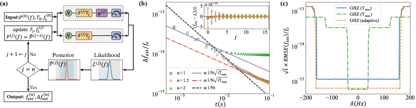
Figure 1: (a) Schematic of ABQFE with two individual GHZ states. A phase difference $\varphi^{(j)}=\pi/2$ is introduced into one state when $T_{j}<T_{max}$. The interrogation time $T_{j}$ is updated with the credible interval (blue region) of the posterior distribution $\tilde{\mathcal{P}}^{(j-1)}(f)$ according to Eq. (5b) and $\tilde{\mathcal{P}}^{(j-1)}(f)$ is inherited as next prior distribution $P^{(j)}(f)$. Meanwhile the LO frequency is varied through $f_{L}^{(j)}=f_{est}^{(j-1)}$ for the next iteration. Here, the detuning $\delta^{(j)}=2\pi(f_{c}-f_{L}^{(j)})$ and $f_{c}\approx 4.295\times 10^{14}$ Hz is chosen as the ${}^{1}{S}_{0}\leftrightarrow{}^{3}{P}_{0}$ clock transition of ⁸⁸Sr  [26]. (b) The standard deviation versus the total interrogation time $t=\sum_{j}{T_{j}}$ for $\alpha=\{1,1.5,2\}$. The dashed line indicates the dual Heisenberg-limited scaling $\propto\frac{1}{Nt}$. The scaling of non-adaptive scheme with $T_{j}=T_{min}$ (purple) and $T_{j}=T_{max}$ (red) is given for comparison. Inset shows the bias versus the Bayesian iteration index $j$. These results are averaged over $R=5000$ simulations with $N_{0}=4,M=9,T_{min}=0.75$ ms, $T_{max}=3$ ms. (c) The RMSE of final estimation versus the initial detuning $\delta=f_{c}-f_{L}^{(0)}$. The interrogation time of non-adaptive scheme is chosen as $n=40,T_{j}=T_{min}=0.75$ ms and $n=10,T_{j}=T_{max}=3$ ms. For the ABQFE, $T_{min}=0.75$ ms, $T_{max}=3$ ms, $\alpha=1,n=13$. Thus, the total interrogation time (30 ms) for the non-adaptive scheme is close to the one (30.18 ms) for the adaptive scheme.

Bayesian quantum estimation provides a powerful tool for optimal high-precision measurements [52, 53, 54, 55, 56, 57, 58, 59, 60, 61, 62, 63, 64, 65, 66, 67]. For a given initial prior distribution $P(f)$, where $f$ represents the unknown frequency to be estimated, one can update the knowledge of this frequency based on the data after each measurement using Bayes’ theorem. Setting the posterior distribution as the next prior distribution, one can implement the Bayesian update iteratively. Suppose $M$ independent measurements are made (or $M$ copies are measured simultaneously), the final posterior distribution can be expressed as

$$\mathcal{P}_{M}(f|N,\varphi,f_{L},T,\mu)=\mathcal{N}\mathcal{L}_{M}(\mu|N,\varphi,f,f_{L},T)P(f),$$ (2)

where $\mathcal{L}_{M}(\mu|N,\varphi,f,f_{L},T)=\binom{M}{\mu}{[\mathcal{L}_{+}]^{\mu}[\mathcal{L}_{-}]^{M-\mu}}$ is a binomial likelihood of measuring $\mu$ times of $u=+1$ and $M-\mu$ times of $u=-1$, and $\mathcal{N}$ is the normalization factor. Then the estimation of $f_{c}$ is given as

$$f_{est}(\mu)=\int{\mathcal{P}_{M}(f|N,\varphi,f_{L},T,\mu)fdf}.$$ (3)

The performance of this estimation can be evaluated by the root mean square error (RMSE) between $f_{est}(\mu)$ and the true value $f_{c}$ under all possible measurements $\mu$,

$$\footnotesize\textrm{RMSE}(f_{est})=\sqrt{\sum_{\mu}{\mathcal{L}_{M}(\mu|N,\varphi,f_{c},f_{L},T)\left[f_{est}(\mu)-f_{c}\right]^{2}}}.$$ (4)

Extending dynamic range via adaptive Bayesian quantum frequency estimation (ABQFE). – In the framework of frequentist measurements based upon individual GHZ states, there is a trade-off between sensitivity and dynamic range. Given the maximum interrogation time $T_{max}$, which is limited by the coherence time, the RMSE of an atomic clock operated with individual $N$-particle GHZ states can only reach the lower bound $1/(2\pi\sqrt{M}NT_{max})$ in a narrow dynamic range with width $1/(2NT_{max})$. By using cascaded GHZ states with small and large particle number $N$, the dynamic range can be extended to $1/(2T_{max})$ [34]. Moreover, the dynamic range can be further improved to $1/T_{max}$ by introducing an auxiliary phase [33, 35].

In parallel with the use of cascaded GHZ states and auxiliary phase, one can utilize ABQFE with short and long interrogation times to extend the dynamic range to $1/(2NT_{min})$, where $T_{min}$ is the minimum available interrogation time for an individual GHZ state. Moreover, integrating ABQFE with cascaded GHZ states and auxiliary phase, the dynamic range can be further extended to $1/T_{min}$ [51]. Below we show how to design and implement the ABQFE for GHZ-state-based atomic clocks.

Generally, the likelihood function and posterior distribution for $K+1$ ensembles is $\tilde{\mathcal{L}}(f)=\prod_{k=0}^{K}{\mathcal{L}_{M_{k}}(\mu_{k}|N_{k},\varphi_{k},f,f_{L},T)}$ and $\tilde{\mathcal{P}}(f)=\tilde{\mathcal{N}}\tilde{\mathcal{L}}(f)P(f)$, where $k=0,1,...,K$ represents different ensembles and $\tilde{\mathcal{N}}$ is the normalization factor. To obtain a doubled dynamic range [35, 33], we first consider the ABQFE for two identical $N$-particle ensembles $(K=1)$ with $M=\sum_{k=0,1}M_{k}$ copies in total, in which $M_{0}=\lfloor\frac{M}{2}\rfloor$ copies is equipped with an auxiliary phase $\varphi_{0}=\varphi$ and $M_{1}-M-M_{0}$ with $\varphi_{1}=0$, as shown in Fig. 1 (a). In our ABQFE, we adaptively adjust the LO frequency according to the posterior distribution during Bayesian updates for clock frequency estimation and locking. Here, we denote the interrogation time in the $j$-th Bayesian update as $T_{j}$, which varies in the interval $T_{min}\leq T_{j}\leq T_{max}$. With Eq. (1), the optimal estimation occurs at $\delta=0$, and the influence of dephasing and detection noises at this point can be reduced [51].

During the adaptive iteration process, only a portion of the credible interval (e.g. $3\Delta f_{est}$ represents the $99.73\%$ credible level of the Gaussian distribution, where $\Delta f_{est}$ is the variance of a posterior distribution) dominates the subsequent Bayesian iteration. Therefore, we can focus solely on that same segment of the likelihood function for the next measurement. The preliminary idea has been used to determine proper execution times in adaptive Bayesian phase estimation with different circuit depths [65]. Differently, here we give an analytic time sequence that can utilize the interrogation time efficiently and provide stable estimation. That is, we set the period of the likelihood function as the width of last posterior credible interval, i.e., $\frac{1}{NT_{j+1}}=2g\Delta f_{est}^{(j)}$, where $g$ is related to the credible interval. Therefore, for $N$-particle GHZ state with $M$ copies in total we can derive the time sequence as

$$T_{j}= T_{min}, j=0$$ , (5a)

$$T_{j}= \min(T_{min}\alpha(1+\alpha^{2})^{\frac{j-1}{2}},\;T_{max}), j\geq 1$$ , (5b)

where $\alpha=\sqrt{M}\pi/{g}$, and $\alpha\geq 1$ ensures $T_{1}\geq T_{min}$. Here, the larger $\alpha$ means faster increasing of $T_{j}$. However, a larger $\alpha$ is more susceptible to random noise. By consulting the t-distribution table [68], we can establish a lower bound for $g$, which in turn provides an upper bound for $\alpha$ [51]. In the following, we choose the most stable case of $\alpha=1$. The time sequence above is predetermined based on the theoretical framework. Alternatively, in realistic applications, the interrogation time $T_{j}$ can also be updated with the realistic variance obtained at each step. It should be mentioned that the auxiliary phase $\varphi^{(j)}=\pi/2$ can only be introduced when $T_{j}<T_{max}$, while for $T_{j}=T_{max}$, it can be turned off with $\varphi^{(j)}=0$.

The LO frequency $f_{L}^{(j)}$ is updated using the previous estimation $f_{est}^{(j-1)}$. This process makes $f_{L}^{(j)}$ gradually approaches $f_{c}$ and ensures that the estimated frequency stays close to the optimal point. The prior distribution is updated based on the posterior distribution from the last measurement, i.e., $P^{(j)}(f)=\tilde{\mathcal{P}}^{(j-1)}(f)$. As $T_{j}$ increases, the period of the likelihood function derived from the measurement results decreases. Thus, the estimation range is updated to $f\in[f_{est}^{(j-1)}-\frac{1}{NT_{j}},f_{est}^{(j-1)}+\frac{1}{NT_{j}}]$, and the previous posterior function is interpolated to update the current prior function [51]. The standard deviation of $f_{est}$ can be analytically obtained by [51],

$$\Delta f^{(j)}_{est}=\frac{1}{2\pi\sqrt{M}N\sqrt{\sum_{i=0}^{j}{T_{i}^{2}}}},$$ (6)

where $t=\sum_{j}T_{j}$ is the total interrogation time. Notably, when $T_{j}<T_{max}$ and $t\gg T_{min}$, we have

$$\Delta f^{(j)}_{est}\approx\frac{1}{2\pi\sqrt{M}Nt}\propto\frac{1}{Nt},$$ (7)

which is a dual Heisenberg-limited scaling versus both particle number $N$ and total interrogation time $t$. Since $T_{j}$ increases to $T_{max}$, $\Delta f^{(j)}_{est}$ will gradually degrade into a hybrid Heisenberg-SQL scaling $\Delta f^{(j)}_{est}\propto{1}/{(N\sqrt{t})}$ [51], which shows Heisenberg scaling with respect to $N$ and SQL scaling with respect to $t$.

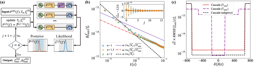
Figure 2: (a) Schematic of ABQFE with cascaded GHZ states. The auxiliary phase is only introduced into the state of smallest particle number $N_{0}$. Similar to Fig. 1, the interrogation times $T_{j}$ are updated according to Eq. (5b), as well as the LO frequency $f_{L}^{(j)}=f_{est}^{(j-1)}$ and the prior distribution $\tilde{\mathcal{P}}^{(j-1)}(f)\rightarrow P^{(j)}(f)$. (b) The standard deviation versus the total interrogation time $t=\sum_{j}{T_{j}}$ for $\alpha=\{1,1.5,2\}$. Here the cascaded GHZ states are set as $\{N_{k}\}=\{1,1,2,4\}$ with $\{M_{k}\}=\{7,7,7,2\}$ to make $N_{t}=36$. (c) The RMSE versus the detuning $\delta$ for different schemes. The minimum and maximum interrogation times are set as $T_{min}=0.75$ ms and $T_{max}=3$ ms, respectively.

Since it is difficult to go through all possible outcomes within the framework of ABQFE, hereafter we use the average of multiple simulation for evaluation. Therefore, the estimated frequency is given as $\bar{f}_{est}^{(j)}=\frac{1}{R}\sum_{r=1}^{R}{[f_{est}^{(j)}]_{r}}$ with $\Delta\bar{f}_{est}^{(j)}=\frac{1}{R}\sqrt{\sum_{r=1}^{R}{\{[f_{est}^{(j)}]_{r}}-\bar{f}_{est}^{(j)}\}^{2}}$ and $RMSE({f}_{est}^{(j)})=\frac{1}{R}\sqrt{\sum_{r=1}^{R}{\{[f_{est}^{(j)}}]_{r}-f_{c}\}^{2}}$. In our simulation, $R$ is chosen as 5000. In Fig. 1 (b), we show the performance of ABQFE using 4-particle GHZ states with different increasing rates $\alpha$. According to Eq. (5b), the time sequence is set with $T_{min}=0.75$ ms and $T_{max}=3$ ms and thus it maintains the same dynamic range as the non-adaptive scheme using spin coherent states (SCSs) with fixed $T_{j}=T_{max}$. The estimated frequency gradually converges to the true value, see the inset of Fig. 1 (b). Before $T_{j}$ increases to $T_{max}$, a dual Heisenberg-limited precision scaling $\Delta\bar{f}_{est}\propto 1/(Nt)$ with respect to both $N$ and $t$ can be achieved. Once $T_{j}$ attains $T_{max}$, the precision scaling becomes $\Delta\bar{f}_{est}\propto 1/(N\sqrt{t})$, which is a hybrid Heisenberg-SQL scaling with Heisenberg scaling versus $N$ and SQL scaling versus $t$. While a larger $\alpha$ may lead to higher efficiency (fewer iteration steps and less dead time), if $T_{j}$ grows too rapidly (e.g., $\alpha=2$), accidental large errors can compromise the estimation, causing the precision to deviate from the theoretical prediction [51].

In the ABQFE process, the LO will continuously adjust to ensure $\delta^{(j)}=2\pi(f_{c}-f^{j}_{L})\rightarrow 0$. Consequently, the dynamic range is determined by $\delta^{(1)}$. In Fig. 1 (c), we utilize the RMSE of the final frequency estimation to assess the dynamic range. It is evident that the adaptive strategy not only achieves superior sensitivity close to frequentist measurements taken with $T=T_{max}$, but also reaches high dynamic range close to frequentist measurements taken with $T=T_{min}$. The ABQFE effectively combines the advantages of both short and long interrogation times, thereby overcoming the trade-off between sensitivity and dynamic range in frequentist measurements with individual GHZ states.

In addition to individual GHZ states, the ABQFE can be implemented using cascaded GHZ states. As shown in Fig. 2 (a), we consider a set of cascaded GHZ states, which consists of $K+1$ different GHZ states (each state has $M_{k}$ copies or is measured $M_{k}$ times, $k=0,1,...,K$). Similar to the ABQFE scheme using individual GHZ states, the adaptive parameter can be given as $\alpha=\frac{\kappa\pi}{g}\sqrt{\frac{N_{t}}{N_{0}}}$ with $N_{t}=\sum_{k}{M_{k}N_{k}}$ and $\kappa=\sqrt{\sum_{k}{M_{k}N_{k}^{2}}/N_{t}}$. Here $\kappa$ ranges from $1$ (SCS) to $\sqrt{N}$ (GHZ), and it can be used to compare the sensitivity of different schemes under the same resource consumption $N_{t}$ [51]. Thus, the uncertainty in ABQFE reads $\Delta f_{est}^{(j)}=\frac{1}{2\pi\kappa\sqrt{N_{t}}\sqrt{\sum_{i=0}^{j}{T_{i}^{2}}}}$. Similar to the scheme without cascade, the ABQFE scheme using cascaded GHZ states not only retains the superior sensitivity of the conventional cascade scheme with $T=T_{max}$, see Fig. 2 (b), but also remains the high dynamic range of the conventional cascade scheme with $T=T_{min}$, see Fig. 2 (c). That is, the ABQFE can also effectively address the trade-off between sensitivity and dynamic range in the conventional scheme using cascaded GHZ states. In particular, through combining cascade and ABQFE, the dynamic range can be further improved $4$ times compared to the ABQFE scheme with individual GHZ states.

To evaluate the clock stability, we calculate the overlapping Allan deviation [69] of the fractional frequency $y=f_{est}/f_{c}$. At each locking cycle, the interrogation time and the prior distribution are reset, while the LO frequency is updated to $f_{est}^{(n)}$ from the previous cycle. Assuming the measurements are implemented with $M$ copies for each step, the time for each locking cycle is $T_{cycle}=\sum_{j=0}^{n}{(T_{j}+T_{D})}$ (where $T_{D}$ is the dead time for each step) [51], the overlapping Allan deviation reads

$$\sigma_{y}(\tau)=\frac{1}{2\pi\kappa\sqrt{N_{t}}f_{c}\sqrt{tT_{max}}}\sqrt{\frac{T_{cycle}}{\tau}},$$ (8)

For comparison, we calculate $\sigma_{y}(\tau)$ for both frequentist and Bayesian schemes with individual and cascaded GHZ states. In our calculation, we choose $n=40$ for $T=T_{min}$ and $n=10$ for $T=T_{max}$. This allows the total interrogation time $t=30$ ms to closely match that of the ABQFE scheme with $n=13$ and $\alpha=1$ where $t\approx 30.18$ ms. Similar to Ref. [34], we set $T_{max}+T_{D}=1.26$ s with the dead time $T_{D}=1.257$ s. Averaging over 1000 simulations, the ABQFE scheme with individual GHZ states yields a stability of $1.3(9)\times 10^{-14}/\sqrt{\tau}$, which is $10.3(2)$ dB lower than the conventional scheme of $T=T_{min}$ and $1.6(3)$ dB higher than the conventional scheme of $T=T_{max}$, see Fig. 3. The ABQFE scheme with cascaded GHZ states yields a stability of $1.9(1)\times 10^{-14}/\sqrt{\tau}$, which is slightly worse than the case of cascaded GHZ states using $T=T_{max}$, but much better than the case of cascaded GHZ states using $T=T_{min}$. When $n$ increases, the stability will gradually resemble that of frequentist measurements using $T=T_{max}$, but $T_{cycle}$ increases.

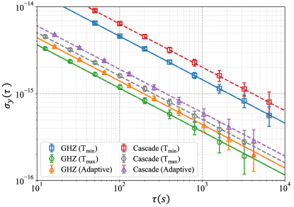
Figure 3: Overlapping Allan deviation versus the average time $\tau$. The two individual GHZ states consist of $N_{k}=\{4,4\},M_{k}=\{4,5\}$, and the cascaded GHZ states are set as $N_{k}=\{1,1,2,4\},M_{k}=\{7,7,7,2\}$. The interrogation time of non-adaptive scheme is chosen as $n=40,T_{j}=T_{min}=0.75$ ms and $n=10,T_{j}=T_{max}=3$ ms. For the ABQFE, we choose $T_{min}=0.75$ ms, $T_{max}=3$ ms, $\alpha=1$, and $n=13$. The data is averaged over $1000$ simulations. The ABQFE with individual GHZ states yields a stability of $1.3(9)\times 10^{-14}/\sqrt{\tau}$, while the corresponding frequentist schemes with $T_{min}$ and $T_{max}$ are respectively $4.5(8)\times 10^{-14}/\sqrt{\tau}$ and $1.1(5)\times 10^{-14}/\sqrt{\tau}$. The ABQFE with cascaded GHZ states yields a stability of $1.9(1)\times 10^{-14}/\sqrt{\tau}$, while the corresponding frequentist schemes with $T_{min}$ and $T_{max}$ are respectively $6.3(8)\times 10^{-14}/\sqrt{\tau}$ and $1.6(0)\times 10^{-14}/\sqrt{\tau}$.

Conclusion and discussion. – In conclusion, we have developed an adaptive Bayesian quantum frequency estimation (ABQFE) scheme that enables high-dynamic-range GHZ-state-based atomic clocks to achieve dual Heisenberg-limited precision scaling. By combining the designed Ramsey interferometry sequence with short and long interrogation times, our ABQFE scheme offers an alternative approach to improve the dynamic range of GHZ-state-based atomic clocks, in parallel with the use of cascaded GHZ states. Notably our ABQFE scheme can achieve dual Heisenberg-limited precision scaling with respect to both particle number and total interrogation time. Moreover, our ABQFE scheme may effectively overcome the trade-off between sensitivity and dynamic range in conventional schemes using individual or cascaded GHZ states. Furthermore, in the framework of Bayesian quantum estimation, we find that employing an interaction-based detection and conducting sign measurements may enhance the robustness of GHZ-state-based atomic clocks against decoherence and detection noises, compared to parity measurements [51]. Building on recent experimental advancements [34, 35, 38], our proposal offers a promising approach for simultaneously achieving high precision and high dynamic range in entanglement-enhanced atomic clocks.

Appendix A I. Detection for GHZ-state-based Ramsey interferometry

In this section, we show how to use practical observable for frequency estimation with GHZ-state-based Ramsey interferometry. In general, one can use parity measurement for detection. Besides, one can also implement an interaction-based readout and use half-population difference measurement for detection. In the following, we show how to use these two protocols for detection.

For an input GHZ state

$$\ket{\psi}_{GHZ}=(\ket{0}^{\otimes N}+\ket{1}^{\otimes N})/\sqrt{2},$$ (S1)

a relative phase $\phi=\delta T$ is collectively accumulated during the Ramsey interrogation, which is governed by Hamiltonian

$$\hat{H}=\delta\hat{J}_{z}.$$ (S2)

Thus, it leads to a $\delta$-dependent output state

$$\ket{\psi(\delta)}_{out}=(\ket{0}^{\otimes N}+e^{iN\delta T}\ket{1}^{\otimes N})/\sqrt{2},$$ (S3)

where $\delta=2\pi(f_{c}-f_{L})$ is the detuning between the LO frequency $f_{L}$ and clock transition frequency $f_{c}$ between $\ket{0}$ and $\ket{1}$, and $T$ the interrogation time. Meanwhile, one may vary the accumulated phase by introducing an auxiliary phase $\varphi=2\pi Nf_{a}T$ which can be realized by adding a frequency shift $f_{a}$ onto the local oscillator frequency.

Within the collective spin representation [5, 39], the eigenvalue of $\hat{J}_{z}$ is represented by the half population difference $m=(N_{\uparrow}-N_{\downarrow})/2$. For an arbitrary quantum state $\ket{\psi}=\sum_{m=-N/2}^{N/2}C_{m}\ket{N/2,m}$, the expectation of an observable $\hat{O}(\hat{J}_{z})$ defined by $\hat{J}_{z}$ can be described as $\langle\hat{O}(m)\rangle=\sum_{m=-N/2}^{N/2}p_{m}O(m)$, where $p_{m}=|C_{m}|^{2}$ is the probability amplitude and $O(m)$ is the eigenvalue of the observable $\hat{O}(\hat{J}_{z})$.

For the parity measurements $\hat{\Pi}=e^{i\pi\lceil\hat{J}_{z}\rceil}$, we only need to perform a $\pi/2$ rotation after accumulating the phases $\phi=\delta T$ with a known auxiliary phase $\varphi$. The output state for measurement can be expressed as

$$\ket{\psi(\delta)}_{\Pi}=e^{-i\frac{\pi}{2}\hat{J}_{y}}e^{-i2\pi f_{a}T\hat{J}_{z}}e^{-i\delta T\hat{J}_{z}}\ket{\psi}_{GHZ}.$$ (S4)

The measurement outcomes for the parity $\hat{\Pi}$ are either odd or even with $u=-1$ and $u=1$, respectively. The correspondent probability for obtaining the odd $(u=-1)$ or even $(u=1)$ parity can be given as

$$\mathcal{L}_{u}\equiv\mathcal{L}(u|N,\varphi,f_{c},f_{L},T)=\frac{1}{2}\{1+C\cdot u(-1)^{N}\cos[2\pi NT(f_{c}-f_{L})+\varphi]\},$$ (S5)

where $C$ is the contrast. The probability is a cosine-type and it would become a sine-type if $\varphi=\pi/2$. According to Eq. (S5), the expectation of the parity measurement can be given as $\langle\hat{\Pi}\rangle=(-1)^{N}C\cdot\cos[2\pi NT(f_{c}-f_{L})+\varphi]$, revisits the well-known result for GHZ state. One can use Eq. (S5) as the binary likelihood to perform the Bayesian estimation.

In parallel to parity measurement, we also find that interaction-based readout can be used for GHZ state detection [47], which has been proved that it is robust to the decoherence induced by spontaneous decay [50]. After the Ramsey interrogation, one can introduce a one-axis twisting dynamics for interaction-based readout. The output state can be expressed as

$$\ket{\psi(\delta)}_{R}=e^{-i\frac{\pi}{2}\hat{J}_{x}^{2}}e^{-i2\pi f_{a}T\hat{J}_{z}}e^{-i\delta T\hat{J}_{z}}\ket{\psi}_{GHZ}$$ (S6)

when $N$ is even. The ideal probability and expectation of half-population difference come out as $p_{\pm\frac{N}{2}}=\frac{1}{2}\{1\pm(-1)^{\lceil\frac{N}{2}+1\rceil}C\cdot\sin[2\pi NT(f_{c}-f_{L})+\varphi]\}$ and $\langle\hat{J}_{z}\rangle=(-1)^{\lceil\frac{N}{2}+1\rceil}\frac{N}{2}C\cdot\sin[2\pi NT(f_{c}-f_{L})+\varphi]$. Besides, one can perform the sign measurement of half-population difference $\hat{S}=Sgn[\hat{J}_{z}]$ to extract the information of $\delta$. The measurement outcomes for sign measurement $\hat{S}$ are either positive or non-positive with $u=1$ and $u=-1$, respectively. The correspondent probability for obtaining the positive $u=+1$ and non-positive $u=-1$ value can be given as

$$\mathcal{L}_{u}\equiv\mathcal{L}(u|N,\varphi,f_{c},f_{L},T)=\frac{1}{2}\{1+C\cdot u(-1)^{\lceil\frac{N}{2}+1\rceil}\sin[2\pi NT(f_{c}-f_{L})+\varphi]\},$$ (S7)

where $C$ is the contrast. The probability is a sine-type here and it would become a cosine-type if $\varphi=\pi/2$. According to Eq. (S7), the expectation of the sign measurement can be given as $\langle\hat{S}\rangle=(-1)^{\lceil\frac{N}{2}+1\rceil}C\cdot\sin[2\pi NT(f_{c}-f_{L})+\varphi]$. The probability and expectation for $N$ is odd remain the same as stated above if we apply an additional rotation, i.e., $\ket{\psi(\delta)}_{R}=e^{-i\frac{\pi}{2}\hat{J}_{y}}e^{-i\frac{\pi}{2}\hat{J}_{x}^{2}}e^{-i2\pi f_{a}T\hat{J}_{z}}e^{-i\delta T\hat{J}_{z}}\ket{\psi}_{GHZ}$.

According to Eqs. (S5) and (S7), both protocols have the similar probabilities. Thus, we adopt a unified form [Eq. (1) in the main text] to express and it can be used as the binary likelihood for Bayesian estimation. For parity measurement, $\xi(N)=(-1)^{N}$. While for interaction-based readout with sign measurement, $\xi(N)=(-1)^{\lceil\frac{N}{2}+1\rceil}$. In ideal cases, the contrast in Eqs. (S5) and (S7) is $C=1$. However, under the influences of dephasing or detection noise, the contrast $C$ will reduce and therefore decrease the measurement precision.

Appendix B II. Influences of dephasing and detection noise

In this section, we show how the dephasing during Ramsey interrogation and detection noise affect the detection, which are the two main limitations for realizing practical GHZ-state-based sensors. Despite both can lead to the contrast reduction, however we find that using interaction-based readout with sign measurement can be much more robust against these noises than using conventional parity measurement.

First, we consider the influence of dephasing during the free Ramsey interrogation process under Hamiltonian of $H_{0}=\delta\hat{J}_{z}$. In the presence of dephasing, the time-evolution of the system can be described by the following master equation [6, 70],

$$\dot{\rho}=-i[\hat{H}_{0},\rho]+\gamma\left(2\hat{L}\rho\hat{L}^{\dagger}-\rho\hat{L}^{\dagger}\hat{L}-\hat{L}^{\dagger}\hat{L}\rho\right),$$ (S8)

where the Lindblad operator $\hat{L}=\hat{J}_{z}$, $\rho$ is the density operator and $\gamma$ is the decay rate of collective dephasing. For processes as in Eq. (S5) and  (S7), the ideal case without dephasing is $\gamma=0$. While in the presence of dephasing with $\gamma>0$, both protocols suffer from a contrast reduction

$$C_{\gamma}=\langle{\hat{O}}\rangle_{\gamma}/\langle{\hat{O}}\rangle_{0}=e^{-\gamma TN^{2}/2},$$ (S9)

where $\langle{\hat{O}}\rangle_{\gamma}=Tr[\rho(T)\hat{O}]$ is the expectation of $\hat{O}$ under dephasing rate $\gamma$.

Both parity measurement $\hat{\Pi}$ and sign measurement $\hat{S}$ are based on the half-population difference $\hat{J}_{z}$, in which one obtain the value of half-population difference $m$ and then convert it into the corresponding parity or sign value. For the detection noise in realistic measurements, we consider an inefficient detector with Gaussian detection noise [48], the probability of obtaining $m$ becomes

$$p_{m}(\sigma_{d})=\sum_{n=-N/2}^{n=N/2}{A_{n}p_{n}e^{-\frac{(m-n)^{2}}{2\sigma_{d}^{2}}}},$$ (S10)

where $\sigma_{d}$ is the intensity of detection noise and $A_{n}=1/\sum_{n=-N/2}^{n=N/2}{p_{n}e^{-\frac{(m-n)^{2}}{2\sigma_{d}^{2}}}}$ is a normalized factor. Thus the contrast under detection noise becomes

$$C_{\sigma_{d}}=\langle{\hat{O}(m)}\rangle_{\sigma_{d}}/\langle{\hat{O}(m)}\rangle_{0},$$ (S11)

where $\langle{\hat{O}(m)}\rangle_{\sigma_{d}}=\sum_{m=-N/2}^{N/2}O(m)p_{m}(\sigma_{d})$ stands for the reduced expectation of $\hat{O}$.

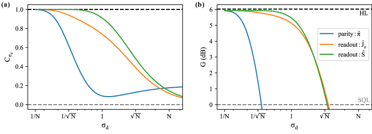
Figure S1: (a) Contrast and (b) Metrological gain versus the intensity of Gaussian detection noise $\sigma_{d}$ for conventional parity measurement and interaction-based readout with sign measurement and half-population difference measurement. Here, the calculation is implemented using GHZ state with $N=4$.

To show the influences of detection noise, we give the comparison on the contrast $C_{\sigma_{d}}$ and the metrological gain $G=20\rm{log}_{10}\left[\Delta f_{GHZ}^{opt}(\sigma_{d})/\Delta f_{SCS}\right]$ using three different detection protocols, one is conventional parity measurement and the others are interaction-based readout with sign measurement and half-population difference measurement. Here the metrological gain refers to the optimal precision compared to the corresponding SQL $\Delta f_{SCS}$, and the optimal precision is calculated by error propagation formula $\Delta f^{opt}=(\Delta\hat{O}/|\partial\langle\hat{O}\rangle/\partial f|)_{f_{opt}}$.

As shown in Fig. S1, it is evident that parity measurement is significantly impacted by detection noise. In contrast, the half-population difference and sign measurement demonstrate strong robustness against detection noise, with the sign measurement being the most effective one among the three methods. Consequently, it is feasible to simplify the probability distribution to a binomial distribution by employing interaction-based readout with sign measurement, thereby facilitating Bayesian estimation. This measurement protocol is robust against detection noise, which is experimentally friendly for implementation.

Since dephasing and detection noise act independently on the contrast, the overall contrast under these noises becomes

$$C(\gamma,T,\sigma_{d})=e^{-\gamma T{N^{2}}/{2}}C_{\sigma_{d}}.$$ (S12)

The influence of dephasing becomes dominated as $N$ gets large, therefore significantly restricting the maximum interrogation time. While for detection noise, the parity measurement places high demands on the detector’s resolution at the single-particle resolved level. In comparison, the interaction-based readout has lower requirements for detector resolution, which enhances its robustness and experimental feasibility under detection noise. We will show the influences of dephasing and detection noise on the uncertainty of frequency estimation below.

Appendix C III. Bayesian estimation using auxiliary phase and cascaded GHZ states

The multi-ensemble cascaded GHZ states are proposed and demonstrated for extending the dynamic range [29, 30, 31, 32, 30, 33, 34, 35]. The key is to use a cascade of GHZ states with different exponentially increasing particle number to update the posterior distribution, in which the overlapping of conditional probabilities with different periods reduces the phase ambiguity. However for sinusoidal probability of Eqs. (S5) and (S7), the frequency can only be uniquely determined for half of a period. To overcome this problem [33], as illustrated in Fig. S2 (a), an auxiliary phase can be introduced in the first ensemble to double the dynamic range.

Assuming that the particle number of ensembles in the cascade grows exponentially, i.e.,

$$N_{k}=2^{k-1}N_{0}\quad(k>1),$$ (S13)

with $M_{k}=M_{K}+v(K-k)$ independent measurements or copies. For the smallest ensembles $N_{1}=N_{0}$, we make $M_{0}=\lfloor\frac{M_{K}+v(K-1)}{2}\rfloor,M_{1}=M_{K}+v(K-1)-M_{0}$. When $K\leq 1$, it returns to the case of individual spin coherent state (SCS) ($N_{k}=1$ returns to an SCS) or GHZ state ($N_{k}>1$). When $\varphi_{k}=0$, it returns to the case without auxiliary phase.

Combining all measurement outcomes of $K+1$ ensembles with different particle number $N_{k}$ ($k=0,...,K$, each with $M_{k}$ copies and $N_{1}=N_{0}$), the likelihood function reads

$$\tilde{\mathcal{L}}(f)=\prod_{k=0}^{K}{\mathcal{L}_{M_{k}}(\mu_{k}|N_{k},\varphi_{k},T,f)},$$ (S14)

where $\mathcal{L}_{M}(\mu|N,\varphi,f_{c},f_{L},T)=\binom{M}{\mu}{[\mathcal{L}_{+}]^{\mu}[\mathcal{L}_{-}]^{M-\mu}}$ is a binomial likelihood of measuring $\mu$ times of $u=+1$ and $M-\mu$ times of $u=-1$, and $\mathcal{N}$ is the normalization factor.

The final posterior distribution given by Bayesian theorem [57, 71] is

$$\tilde{\mathcal{P}}(f)=\mathcal{N}\tilde{\mathcal{L}}(f)P(f).$$ (S15)

Thus, the estimated frequency

$$f_{est}(\{\mu_{k}\})=\int{\tilde{\mathcal{P}}(f)fdf},$$ (S16)

and the corresponding RMSE

$$RMSE(f_{est})=\sqrt{\sum_{\{\mu_{k}\}}\tilde{\mathcal{L}}(f_{c})[f_{est}(\{\mu_{k}\})-f_{c}]^{2}}.$$ (S17)

The case without auxiliary phase should require a Gaussian distribution $P(f)=\frac{1}{\sqrt{2\pi}\sigma_{f}}\exp(-\frac{f_{c}^{2}}{2\sigma_{f}^{2}})$ as the prior [34], or limit the range within half a period $f\in[f_{L}-\frac{1}{2N_{0}T},f_{L}+\frac{1}{2N_{0}T}]$ when calculate the posterior. Details are shown in Table S1. Differently, here we realize the full period estimation by using an auxiliary phase. In this case we only need to select the smallest ensemble $N_{0}$ and introduce the additional phase $\varphi_{0}=\pi/2$ to perform the first measurement and then use the cascaded GHZ states with $\varphi_{k}=0$ ($k=1,2,...,K$) for subsequent Bayesian updates. Since the auxiliary phase is present, a uniform prior distribution $P(f)=1/T$ is sufficient. In practice, it is more appropriate to use the uniform prior distribution when the phase to be estimated is completely unknown.

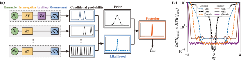
Figure S2: (a) Schematic of multi-ensemble Bayesian frequency estimation with auxiliary phase shift. Here, $N_{k}$ stands for particle number of the $k$-th ensemble ($k=0,...,K$, each with $M_{k}$ copies), $\delta=2\pi(f_{c}-f_{L})$ and $T$ is the interrogation time, $f_{est}$ is the estimated value for $f_{c}$, $\varphi_{0}$ is the introduced auxiliary phase. (b) The RMSE versus $\delta T$ for different strategies. With auxiliary phase $\varphi_{0}=\pi/2$, the prior distribution can be flat. For fair comparison, $N_{k}$ and $M_{k}$ are selected to keep $N_{t}=\sum_{k}N_{k}M_{k}$ almost the same. For SCS, $N_{0}=N_{1}=1$ with $M_{0}=M_{1}=59$. For GHZ state, $N_{0}=N_{1}=8$ with $M_{0}=7,M_{1}=8$. For cascaded GHZ states, $\{N_{k}\}=\{1,1,2,4,8\}$ with $\{M_{k}\}=\{13,13,18,10,2\}$. While for the cases without auxiliary phase ($k=1,...,K$), the prior distribution should change to a Gaussian function [34]. For SCS, $N_{1}=1$ with $M_{1}=118$. For GHZ state, $N_{1}=8$ with $M_{1}=15$. For cascaded GHZ states, $\{N_{k}\}=\{1,2,4,8\}$ with $\{M_{k}\}=\{26,18,10,2\}$.

The uncertainty of the estimator is quantified its variance,

$$\Delta^{2}{f}_{est}=\sum_{\{\mu_{k}\}}{\tilde{\mathcal{L}}(f_{c})[f_{est}-\bar{f}_{est}]^{2}df},$$ (S18)

where

$$\bar{f}_{est}=\sum_{\{\mu_{k}\}}{\mathcal{L}(f_{c})f_{est}(\{\mu_{k}\})}$$ (S19)

is the expectation of estimation under all possible measurements. The bias assesses the accuracy of an estimator, while the variance assesses the precision of the estimator.

Thus the RMSE consists of both the bias $\bar{f}_{est}-f_{c}$ and variance $(\Delta^{2}f_{est})$, i.e.,

$$RMSE(f_{est})=\sqrt{|\bar{f}_{est}-f_{c}|^{2}+\left(\Delta^{2}f_{est}\right)},$$ (S20)

It is known that $RMSE(f_{est})\geq\Delta f_{est}\geq\Delta f_{CRLB}$, where

$$\Delta^{2}f_{CRLB}=\frac{\left(\frac{d\bar{f}_{est}}{df_{c}}\big{|}_{f_{c}}\right)^{2}}{F(f_{c})}$$ (S21)

is the Cramer-Rao lower bound, and

$$F(f_{c})=\sum_{\{\mu\}}{\frac{1}{\tilde{\mathcal{L}}(f)}\left(\frac{\partial{\tilde{\mathcal{L}}(f)}}{\partial f}\bigg{|}_{f_{c}}\right)^{2}}$$ (S22)

is the Fisher information.

Consider the cascaded GHZ states that has $(K+1)$ ensembles arranged from $k=0$ to $k=K$, in which each ensemble carries $M_{k}$ copies of GHZ state with $N_{k}$ qubits. For each ensemble, when the number of measurements $M_{k}$ is large, the posterior distribution approaches a Gaussian distribution $\mathcal{G}(f_{c},\Delta\sigma_{k})$, where $\sigma_{k}=1/(2\pi T\sqrt{M_{k}N_{k}^{2}})$. When the results of these ensembles are combined together, it is equivalent to multiply their likelihood functions, and ideally the resulting posterior distribution is also a Gaussian distribution whose standard deviation becomes $\Delta f_{est}=\sqrt{1/\sum_{k}{\sigma_{k}^{2}}}$. Theoretically, when the interrogation time is fixed with $T$, the optimal lower bound of the posterior standard deviation is

$$\Delta f_{est}=\frac{1}{2\pi T\sqrt{\sum_{k}{M_{k}N_{k}^{2}}}}=\frac{1}{2\pi T\kappa\sqrt{N_{t}}},$$ (S23)

which is a general expression that works for both cascading and non-cascading scenarios. Here $N_{t}=\sum_{k}{M_{k}N_{k}}$, and $\kappa^{2}=\sum_{k}^{K}{M_{k}N_{k}^{2}}/N_{t}$. From Eq. (S23), we can see that the factor $\kappa$ can be used to compare the lower bounds of different schemes under the same resource consumption $N_{t}$. For SCS, $\kappa=1$ and for GHZ state, $\kappa=\sqrt{N_{GHZ}}$ where $N_{GHZ}$ is the particle number of a GHZ state. As shown in Fig. S2 (b), the dynamic range with auxiliary phase is twice as that without auxiliary phase for all states as in Table. S1. Although the RMSE is slightly increased in some specific points, the application of $\varphi_{0}=\pi/2$ does double the dynamic range compared to the ones without auxiliary phase. Moreover, with cascaded GHZ state, the dynamic range is extended further.

States	Auxiliary phase	$\{N_{k}\}$	$\{M_{k}\}$	$\varphi_{0}$	Prior
SCS	without	$\{1\}$	$\{118\}$	$0$	Gaussian
	with	$\{1,1\}$	$\{59,59\}$	$\pi/2$	flat
GHZ	without	$\{8\}$	$\{15\}$	$0$	Gaussian
	with	$\{8,8\}$	$\{7,8\}$	$\pi/2$	flat
Cascaded GHZ	without	$\{1,2,4,8\}$	$\{26,18,10,2\}$	$0$	Gaussian
	with	$\{1,1,2,4,8\}$	$\{13,13,18,10,2\}$	$\pi/2$	flat

Table S1: Details of setting with or without the auxiliary phase using three typical quantum states: SCS, GHZ state and cascaded GHZ states. See RMSE of those in Fig. S2 (b).

Appendix D IV. Design of time sequence and uncertainty in ABQFE

In this section, we show how to design the time sequence for Bayesian estimation and the analytical analysis on the uncertainty. Based on the general expression Eq. (S23) of posterior standard deviation and considering within the adaptive framework, the standard deviation of the posterior distribution at the $j$-th step can be derived from all previous posterior distributions [38], so it can analytically be calculated as

$$\Delta f^{(j)}_{est}=\frac{1}{2\pi\kappa\sqrt{N_{t}}\sqrt{\sum_{i=0}^{j}{T_{i}^{2}}}},$$ (S24)

Note that this is the general description including the cascaded GHZ states, individual GHZ state ($\kappa=\sqrt{N_{GHZ}}$) and SCS ($\kappa=1$).

For the posterior distribution in $j$-th step, the effective information is concentrated in its credible interval. So, when updating the posterior to a prior, only this part plays a role in the subsequent results. We use this idea for atomic clock locking. Difference from the preliminary one that used in quantum circuits by an adaptive Bayesian phase estimation algorithm to design proper circuit depth and execution times [65], here we give an analytic time sequence in terms of the ideal posterior standard deviation. At the $j$-th step, we take a range with $2g\Delta f_{est}^{(j)}$ width as its credible interval, so that when this width equal to the period at next step, i.e., $2g\Delta f_{est}^{(j)}=\frac{1}{N_{0}T_{j+1}}$, we can update with most of the information to the next prior. According to this update idea, in an ideal situation we can obtain the time sequence as

$$T_{j}= T_{min} j<1$$ , (S25a)

$$T_{j}= \min(T_{min}\alpha(1+\alpha^{2})^{\frac{j-1}{2}},\;T_{max}) j\geq 1$$ , (S25b)

where $\alpha=\frac{\kappa\pi}{g}\sqrt{\frac{N_{t}}{N_{0}}}$, and it should be restricted as $\alpha\geq 1$ to make sure $T_{1}\geq T_{min}$. On the other hand, the value of factor $g$ cannot be too small; otherwise, the measured information will be lost. When the sample size is small, $g$ can be determined by consulting the t-distribution table [68]. For example, we choose $M=9$ copies for the measurement of the $N=4$ GHZ state in main text, resulting in 8 degrees of freedom. If the significance level for a two-tailed test is less than $0.001$, then g must be greater than $5.041$, which means $\alpha$ should be restricted as $\alpha\leq 1.86$.

As the interrogation time $T_{j}$ grows as Eq. (S25b), the theoretical standard deviation as in Eq. (S24) thus show different trends versus total interrogation time $t=\sum_{j}T_{j}$, i.e.,

$$\Delta f_{est}= \frac{1}{2\pi\kappa\sqrt{N_{t}}}\frac{1}{T_{min}+(t-T_{min})(\sqrt{1+\alpha^{-2}}-1)} T_{j}\leq T_{max}$$ , (S26a)

$$\Delta f_{est}= \frac{1}{2\pi\kappa\sqrt{N_{t}}}\frac{1}{\sqrt{tT_{max}}} T_{j}>T_{max}$$ , (S26b)

The scaling of the standard deviation versus total interrogation time $\propto 1/t$ when $T_{j}\leq T_{max}$ ($t\gg T_{min}$). When inputting an GHZ state with particle number $N$, the standard deviation exhibits a dual Heisenberg scaling $\propto 1/(Nt)$ of total interrogation time $t$ and particle number $N$ .

When designing the time sequence, we set the credible interval width to $g$ times of the theoretical standard deviation, which provides us with the parameter $\alpha$ to assess the rate of growth of the time sequence. Fewer steps are required to reach $T_{max}$ when $\alpha$ is large, which can theoretically lead to a relatively lower uncertainty. However, this process can also be prone to random errors. If measurements in one step are inaccurate, it will cause significant deviations in all subsequent estimates.

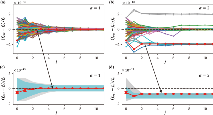
Figure S3: Effects of random noise on frequency estimation results with ABQFE time sequence using $\alpha=1$ and $\alpha=2$. (a-b) Fractional frequency estimation bias $(f_{est}-f_{c})/f_{c}$ versus Bayesian iteration steps $j$. The simulation results are generated under $5000$ different random seeds for each parameter $\alpha$. The first simulated values of different $\alpha$ under the same seed are the same. (c-d) The $1470$-th estimation (red) in (a-b), where the gray area represents the estimate range at the present step and the cyan area represents the estimate range at the next step.

As illustrated in Fig. S3, we present the results of $5000$ simulations conducted under different rates of $\alpha=1,2$, each utilizing the same simulation seed. This approach ensures that the measurements and estimates obtained in the initial step remain consistent. When $\alpha$ is large ($\alpha=2$), the fast increasing of $T_{j}$ can result in unstable estimates. Here, we specifically outline the estimation process for the $1470$-th group for comparison. The time sequence for this group exhibits a faster growth rate when $\alpha=2$. Consequently, when we update the estimation range due to the unsatisfactory results of the initial measurements, the true value appears outside the edges of the estimation range in the second step. As a result, the center of the estimation gradually shifts toward a false true value, which is a multiple of the difference period from the actual true value. While for small rate $\alpha=1$, the results are more stable and the estimated value converges to the true value gradually.

If the influences of dephasing and detection noise are taken into account, the uncertainty and the stability both decrease. As shown in Fig. S4, under dephasing and detection noise, ABQFE can still accurately extract the clock frequency, and $f_{est}$ gradually converges to the true value $f_{c}$. However, since the contrast reduces as Eq. (S9), the uncertainty under these noises becomes

$$\Delta f_{est}^{{}^{\prime}}=\Delta f_{est}/C^{2}(\gamma,T,\sigma_{d}).$$ (S27)

We referred to the experimental results from Ref. [34] and set the parameters to achieve the same contrast in our simulation. For individual GHZ state with $N=4$, we set $\gamma=2.547$ and $C_{\sigma_{d}}=0.938$, which results in a consistent contrast of $C=0.88(2)$ for $T=3$ ms. For ABQFE, the process begins with an interrogation time of $T_{min}=0.75$ ms and initial contrast is $C=0.92(4)$, which decreases to $C=0.88(2)$ as the interrogation time $T_{j}$ increases. In addition, we also give a worse case of $C=0.62(9)$, which is under severe dephasing and detection noise with $\gamma=10,C_{\sigma_{d}}=0.8$ for comparison.

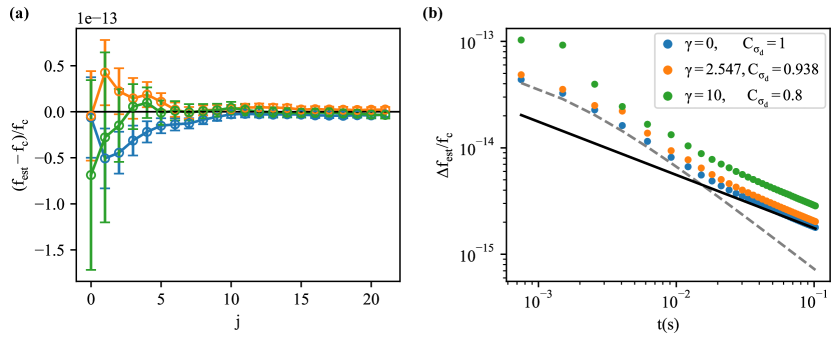
Figure S4: (a) Bias versus Bayesian iteration steps $j$. (b) Uncertainty of fractional frequency versus total interrogation time $t$. Simulations are implemented with $N_{k}=\{4,4\},M_{k}=\{4,5\},\varphi_{0}=\pi/2,\alpha=1$. Here, we present the results with $\gamma=2.547,C_{\sigma_{d}}=0.938$ (orange). We also give the results of ideal case without dephasing and detection noise $\gamma=0,C_{\sigma_{d}}=1$ (blue), and the worse case with $\gamma=10,C_{\sigma_{d}}=0.8$ (green) for comparison. The dashed line presents the theoretical scaling as Eq. (S26a) and the solid line presents the theoretical scaling as Eq. (S26b).

Appendix E V. Atomic clock using ABQFE and the analysis of sensitivity and stability

The clock frequency is locked by the output of an ABQFE cycle, which consist $n$ steps of adaptive measurements. To evaluate the sensitivity, we give the sensitivity of the fractional frequency $y=f_{est}/f_{c}$ after different steps of ABQFE cycling. At each cycle of locking, the interrogation time and the prior distribution are reset, while the LO frequency is updated by $f_{est}^{(n)}$ from the previous cycle. As shown in Fig. S5, assuming the measurements of $N_{k}$ ensembles in ABQFE are implemented with $M_{k}$ copies for each step, the time for each locking cycle is

$$T_{cycle}=\sum_{j=0}^{n}{(T_{j}+T_{D})},$$ (S28)

where $T_{D}$ is the dead time for each step, and $t=\sum_{j=0}^{n}{T_{j}}$ is the total interrogation time that determine the uncertainty of output estimation in one cycle as Eq. (S26b).

Considering the dead time, the sensitivity is determined by the output of an ABQFE cycle, i.e.,

$$\bar{\eta}=\frac{\Delta\bar{f}_{est}}{f_{c}}\sqrt{T_{cycle}}.$$ (S29)

Meanwhile, the overlapping Allan deviation theoretically reads [69]

$$\sigma_{y}(\tau)=\frac{1}{2\pi\kappa\sqrt{N_{t}}f_{c}\sqrt{tT_{max}}}\sqrt{\frac{T_{cycle}}{\tau}},$$ (S30)

which can be utilized to characterize stability. Here $\tau$ represents the total average time of the locking process, including multiple cycles.

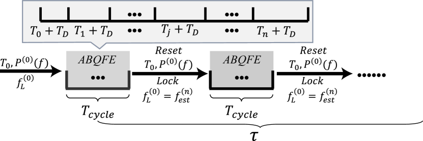
Figure S5: The locking process of an atomic clock that utilizes adaptive Bayesian quantum frequency estimation (ABQFE) involves an interrogation time that increases from $T_{min}$ to $T_{n}$. Here, the dead time for other processes, including preparation and measurements, is denoted as $T_{D}$. The ABQFE spends $T_{cycle}$ to obtain the estimation $f_{est}^{(n)}$ for LO and resets the conditions for the next ABQFE.

We first show the sensitivity during a clock cycle. As shown in Fig. S6, as the number of iterations $n$ increases, $T_{cycle}$ gradually increases, and the sensitivity of an ABQFE cycle gradually improves from the short interrogation time $T_{min}$ to the long interrogation time $T_{max}$. However, the increase in sensitivity gradually slows down, and an excessive number of cycles can lead to prolonged cycle times. Therefore, we can select a moderate number of cycles for clock locking, such as using $n=13$ as mentioned in main text.

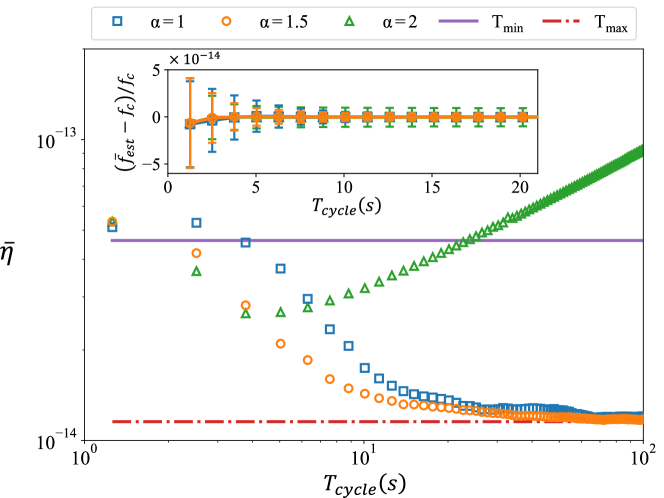
Figure S6: The sensitivity of the ABQFE versus time $T_{cycle}$ during a cycle. We utilize the same settings as shown in Fig. 1 (b) in the main text and take the dead time into account. Here we still give results with different increasing rate $\alpha=1,1.5,2$, and the sensitivities with fixed interrogation time $T_{min}$ (purple) and $T_{max}$ (red) are also given for comparison.

Similarly, stability also decreases in the presence of noises. As shown in Fig. S7, we add the above mentioned dephasing and detection noise $\gamma=2.547,C_{\sigma_{d}}=0.938$ to the ideal case of no-cascaded GHZ state in Fig. 3 for comparison. The simulation results show that the overlapping Allan deviation of each case has a different amplitude increase, that is, the stability decreases. Even so, the adaptive framework still provides overlapping Allan deviation lower than the SQL, both for GHZ states with non-adaptive and adaptive protocols. In average of $1000$ simulations under noisy scenarios, stability of GHZ state with fixed interrogation time $T_{min}=0.75$ms is $5.0(2)\times 10^{-14}/\sqrt{\tau}$, stability of GHZ state with fixed interrogation time $T_{max}=3$ms is $1.3(7)\times 10^{-14}/\sqrt{\tau}$, stability of GHZ state using ABQFE with $\alpha=1$ is $1.6(4)\times 10^{-14}/\sqrt{\tau}$. They are $0.7(8)$ dB, $1.4(7)$ dB and $1.3(9)$ dB higher than their corresponding ideal simulation results, respectively.

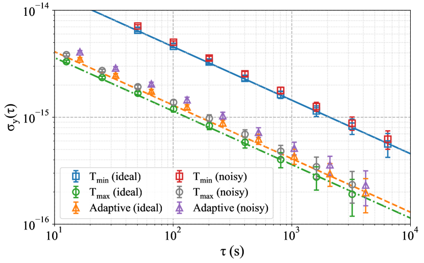
Figure S7: Overlapping Allan deviation of fractional frequency versus $\tau$ under dephasing and detection noise, compared with the ideal case of no-cascaded GHZ state in Fig. 3 in the main text. The noisy case are set up as the ideal case, except for the addition of dephasing $\gamma=2.547$ and detection noise $C_{\sigma_{d}}=0.938$. Compared to the ideal simulations, $\sigma_{y}(\tau)$ for non-adaptive scheme with $T_{j}=T_{min}=0.75$ms (red) is $0.7(8)$ dB higher, for non-adaptive scheme with $T_{j}=T_{max}=3$ms (grey) is $1.4(7)$ dB higher, and for ABQFE (purple) is $1.3(9)$ dB higher.

Appendix F VI. Flowing chart of ABQFE

In this section, we present the basic procedure of the adaptive Bayesian quantum frequency estimation in the flowing chart form shown below.

Input : minimum interrogation time $T_{min}$; maximum interrogation time $T_{\rm max}$; ABQFE iteration steps $n$; Lock steps $n_{L}$; time sequence factor $\alpha$; (K+1) Ensembles $\{N_{k}\},\{M_{k}\}$;

[Bayesian Locking loop]:

for $i=0$ to $n_{L}$ do

       Initialize : initial interval $f=[f_{l},f_{r}]$; initial $\tilde{\mathcal{P}}(f)=1/N_{0}T_{min}$; initial $f_{est}=0$ ;

       [Adaptive Bayesian Update Loop]:

       for $j=0$ to $n$ do

             [Updates of parameter];

             interrogation time: $T=\left\{\begin{array}[]{ll}T_{min},&j=0\\ \min(T_{min}\alpha(1+\alpha^{2})^{\frac{j-1}{2}},\;T_{max})&,j\geq 1\end{array}\right.$ ;

             length of interval: $f_{lr}=1/N_{0}T$;

             if $T_{min}<T<T_{max}$ then

                   $f_{l}^{{}^{\prime}}\leftarrow$ max$(f_{\rm est}-f_{lr}/2,f_{l}$);

                   $f_{r}^{{}^{\prime}}\leftarrow$ min$(f_{\rm est}+f_{lr}/2,f_{r})$;

                   update the prior distribution by interpolating the last posterior distribution in new interval $f^{\prime}=[f_{l}^{{}^{\prime}},f_{r}^{{}^{\prime}}]$;

                   $P(f^{\prime})=$ Interpolate$[\tilde{\mathcal{P}}(f)]$;

                   $f\leftarrow f^{\prime}$;

                  

            else

                   $P(f)=\tilde{\mathcal{P}}(f)$;

                  

             end if

            LO frequency: $f_{L}=f_{est}$;

             Auxiliary phase compensation: $\varphi_{0}=\left\{\begin{array}[]{ll}\pi/2,&T<T_{max}\\ 0,&T=T_{max}\end{array}\right.$ ;

             [Experimental measurement];

             measurement outcome $\{\mu_{k}\}$ from (K+1) ensembles;

             [Bayesian iteration];

             Likelihood function: $\tilde{\mathcal{L}}(f)=\prod_{k=0}^{K}{\mathcal{L}(\mu_{k}|N,\varphi_{k},f,f_{L},T)}$ ;

             Bayesian update: $\tilde{\mathcal{P}}(f)=\tilde{\mathcal{N}}\tilde{\mathcal{L}}(f)P(f)$;

             Estimated frequency: $f_{\rm est}=\int{\tilde{\mathcal{P}}(f)f\mathrm{d}f}$;

             Uncertainty: $\Delta f_{\rm est}=\sqrt{\int{\tilde{\mathcal{P}}(f)(f-f_{\rm est})^{2}}\mathrm{d}f}$;

             Output : estimated frequency $f_{\rm est}$; uncertainty $\Delta f_{\rm est}$.

            

       end for

      Locking the LO frequency to the clock transition frequency via the error signal $f_{\rm est}^{i}-f_{\rm est}^{i-1}$.

end for

Algorithm 1 Flowing chart of our Adaptive Bayesian frequency estimation (ABQFE)

Alternatively, the interrogation time $T_{j}$ in realistic applications can also be updated with the realistic variance obtained at each step, that is

$$T=\left\{\begin{array}[]{ll}T_{min}&,\;j=0\\ \min(\frac{1}{2gN_{0}\Delta f_{est}},\;T_{max})&,\;j\geq 1\end{array}\right.\;$$ (S33)

where $g$ can then be determined according to the t-distribution table.

References

- Degen et al. [2017] C. L. Degen, F. Reinhard, and P. Cappellaro, Quantum sensing, Rev. Mod. Phys. 89, 035002 (2017).
- Ye and Zoller [2024] J. Ye and P. Zoller, Essay: Quantum sensing with atomic, molecular, and optical platforms for fundamental physics, Phys. Rev. Lett. 132, 190001 (2024).
- Huang et al. [2024] J. Huang, M. Zhuang, and C. Lee, Entanglement-enhanced quantum metrology: From standard quantum limit to heisenberg limit, Appl. Phys. Rev. 11, 031302 (2024).
- Greenberger et al. [1989] D. M. Greenberger, M. A. Horne, and A. Zeilinger, Going beyond bell’s theorem, in Bell’s Theorem, Quantum Theory and Conceptions of the Universe, edited by M. Kafatos (Springer Netherlands, Dordrecht, 1989) pp. 69–72.
- Pezzè et al. [2018] L. Pezzè, A. Smerzi, M. K. Oberthaler, R. Schmied, and P. Treutlein, Quantum metrology with nonclassical states of atomic ensembles, Rev. Mod. Phys. 90, 035005 (2018).
- Huelga et al. [1997] S. F. Huelga, C. Macchiavello, T. Pellizzari, A. K. Ekert, M. B. Plenio, and J. I. Cirac, Improvement of frequency standards with quantum entanglement, Phys. Rev. Lett. 79, 3865 (1997).
- Giovannetti et al. [2004] V. Giovannetti, S. Lloyd, and L. Maccone, Quantum-enhanced measurements: Beating the standard quantum limit, Science 306, 1330 (2004).
- Giovannetti et al. [2006] V. Giovannetti, S. Lloyd, and L. Maccone, Quantum metrology, Phys. Rev. Lett. 96, 010401 (2006).
- Lee [2006] C. Lee, Adiabatic mach-zehnder interferometry on a quantized bose-josephson junction, Phys. Rev. Lett. 97, 150402 (2006).
- Chen et al. [2010] Y.-A. Chen, X.-H. Bao, Z.-S. Yuan, S. Chen, B. Zhao, and J.-W. Pan, Heralded generation of an atomic noon state, Phys. Rev. Lett. 104, 043601 (2010).
- Monz et al. [2011] T. Monz, P. Schindler, J. T. Barreiro, M. Chwalla, D. Nigg, W. A. Coish, M. Harlander, W. Hänsel, M. Hennrich, and R. Blatt, 14-qubit entanglement: Creation and coherence, Phys. Rev. Lett. 106, 130506 (2011).
- Giovannetti et al. [2011] V. Giovannetti, S. Lloyd, and L. Maccone, Advances in quantum metrology, Nat. Photonics 5, 222 (2011).
- Zhao et al. [2021] Y. Zhao, R. Zhang, W. Chen, X.-B. Wang, and J. Hu, Creation of greenberger-horne-zeilinger states with thousands of atoms by entanglement amplification, npj Quantum Inf. 7, 24 (2021).
- Ludlow et al. [2015] A. D. Ludlow, M. M. Boyd, J. Ye, E. Peik, and P. O. Schmidt, Optical atomic clocks, Rev. Mod. Phys. 87, 637 (2015).
- Madjarov et al. [2019] I. S. Madjarov, A. Cooper, A. L. Shaw, J. P. Covey, V. Schkolnik, T. H. Yoon, J. R. Williams, and M. Endres, An atomic-array optical clock with single-atom readout, Phys. Rev. X 9, 041052 (2019).
- Origlia et al. [2018] S. Origlia, M. S. Pramod, S. Schiller, Y. Singh, K. Bongs, R. Schwarz, A. Al-Masoudi, S. Dörscher, S. Herbers, S. Häfner, U. Sterr, and C. Lisdat, Towards an optical clock for space: Compact, high-performance optical lattice clock based on bosonic atoms, Phys. Rev. A 98, 053443 (2018).
- Lu et al. [2023] X. Lu, F. Guo, Y. Wang, Q. Xu, C. Zhou, J. Xia, W. Wu, and H. Chang, Absolute frequency measurement of the87 sr optical lattice clock at ntsc using international atomic time, Metrologia 60, 015008 (2023).
- Zhang et al. [2022] A. Zhang, Z. Xiong, X. Chen, Y. Jiang, J. Wang, C. Tian, Q. Zhu, B. Wang, D. Xiong, L. He, L. Ma, and B. Lyu, Ytterbium optical lattice clock with instability of order , Metrologia 59, 065009 (2022).
- Yin et al. [2022] M.-J. Yin, X.-T. Lu, T. Li, J.-J. Xia, T. Wang, X.-F. Zhang, and H. Chang, Floquet engineering hz-level rabi spectra in shallow optical lattice clock, Phys. Rev. Lett. 128, 073603 (2022).
- Li et al. [2024] J. Li, X.-Y. Cui, Z.-P. Jia, D.-Q. Kong, H.-W. Yu, X.-Q. Zhu, X.-Y. Liu, D.-Z. Wang, X. Zhang, X.-Y. Huang, M.-Y. Zhu, Y.-M. Yang, Y. Hu, X.-P. Liu, X.-M. Zhai, P. Liu, X. Jiang, P. Xu, H.-N. Dai, Y.-A. Chen, and J.-W. Pan, A strontium lattice clock with both stability and uncertainty below , Metrologia 61, 015006 (2024).
- Aeppli et al. [2024] A. Aeppli, K. Kim, W. Warfield, M. S. Safronova, and J. Ye, Clock with systematic uncertainty, Phys. Rev. Lett. 133, 023401 (2024).
- Borregaard and Sørensen [2013a] J. Borregaard and A. S. Sørensen, Near-heisenberg-limited atomic clocks in the presence of decoherence, Phys. Rev. Lett. 111, 090801 (2013a).
- Pedrozo-Peñafiel et al. [2020] E. Pedrozo-Peñafiel, S. Colombo, C. Shu, A. F. Adiyatullin, Z. Li, E. Mendez, B. Braverman, A. Kawasaki, D. Akamatsu, Y. Xiao, and V. Vuletić, Entanglement on an optical atomic-clock transition, Nature 588, 414 (2020).
- Schulte et al. [2020] M. Schulte, C. Lisdat, P. O. Schmidt, U. Sterr, and K. Hammerer, Prospects and challenges for squeezing-enhanced optical atomic clocks, Nat. Commun. 11, 5955 (2020).
- Colombo et al. [2022a] S. Colombo, E. Pedrozo-Peñafiel, and V. Vuletić, Entanglement-enhanced optical atomic clocks, Appl. Phys. Lett. 121, 210502 (2022a).
- Eckner et al. [2023] W. J. Eckner, N. Darkwah Oppong, A. Cao, A. W. Young, W. R. Milner, J. M. Robinson, J. Ye, and A. M. Kaufman, Realizing spin squeezing with rydberg interactions in an optical clock, Nature 621, 734 (2023).
- Franke et al. [2023] J. Franke, S. R. Muleady, R. Kaubruegger, F. Kranzl, R. Blatt, A. M. Rey, M. K. Joshi, and C. F. Roos, Quantum-enhanced sensing on optical transitions through finite-range interactions, Nature 621, 740 (2023).
- Robinson et al. [2024] J. M. Robinson, M. Miklos, Y. M. Tso, C. J. Kennedy, T. Bothwell, D. Kedar, J. K. Thompson, and J. Ye, Direct comparison of two spin-squeezed optical clock ensembles at the level, Nat. Phys. 20, 208 (2024).
- Berry et al. [2009] D. W. Berry, B. L. Higgins, S. D. Bartlett, M. W. Mitchell, G. J. Pryde, and H. M. Wiseman, How to perform the most accurate possible phase measurements, Phys. Rev. A 80, 052114 (2009).
- Kessler et al. [2014] E. M. Kessler, P. Kómár, M. Bishof, L. Jiang, A. S. Sørensen, J. Ye, and M. D. Lukin, Heisenberg-limited atom clocks based on entangled qubits, Phys. Rev. Lett. 112, 190403 (2014).
- Kómár et al. [2014] P. Kómár, E. M. Kessler, M. Bishof, L. Jiang, A. S. Sørensen, J. Ye, and M. D. Lukin, A quantum network of clocks, Nat. Phys. 10, 582 (2014).
- Higgins et al. [2009] B. L. Higgins, D. W. Berry, S. D. Bartlett, M. W. Mitchell, H. M. Wiseman, and G. J. Pryde, Demonstrating heisenberg-limited unambiguous phase estimation without adaptive measurements, New J. Phys. 11, 073023 (2009).
- Liu et al. [2023] L.-Z. Liu, Y.-Y. Fei, Y. Mao, Y. Hu, R. Zhang, X.-F. Yin, X. Jiang, L. Li, N.-L. Liu, F. Xu, Y.-A. Chen, and J.-W. Pan, Full-period quantum phase estimation, Phys. Rev. Lett. 130, 120802 (2023).
- Cao et al. [2024] A. Cao, W. J. Eckner, T. Lukin Yelin, A. W. Young, S. Jandura, L. Yan, K. Kim, G. Pupillo, J. Ye, N. Darkwah Oppong, and A. M. Kaufman, Multi-qubit gates and schrödinger cat states in an optical clock, Nature 634, 315 (2024).
- Finkelstein et al. [2024] R. Finkelstein, R. B.-S. Tsai, X. Sun, P. Scholl, S. Direkci, T. Gefen, J. Choi, A. L. Shaw, and M. Endres, Universal quantum operations and ancilla-based read-out for tweezer clocks, Nature 634, 321 (2024).
- [36] S. Direkci, R. Finkelstein, M. Endres, and T. Gefen, Heisenberg-limited bayesian phase estimation with low-depth digital quantum circuits, arxiv:2407.06006 .
- Borregaard and Sørensen [2013b] J. Borregaard and A. S. Sørensen, Efficient atomic clocks operated with several atomic ensembles, Phys. Rev. Lett. 111, 090802 (2013b).
- Han et al. [2024] C. Han, Z. Ma, Y. Qiu, R. Fang, J. Wu, C. Zhan, M. Li, J. Huang, B. Lu, and C. Lee, Atomic clock locking with bayesian quantum parameter estimation: Scheme and experiment, Phys. Rev. Applied 22, 044058 (2024).
- Biedenharn and Louck [1984] L. C. Biedenharn and J. D. Louck, Angular Momentum in Quantum Physics: Theory and Application, Encyclopedia of Mathematics and its Applications (Cambridge University Press, 1984).
- Bollinger et al. [1996] J. J. Bollinger, W. M. Itano, D. J. Wineland, and D. J. Heinzen, Optimal frequency measurements with maximally correlated states, Phys. Rev. A 54, R4649 (1996).
- Campos et al. [2003] R. A. Campos, C. C. Gerry, and A. Benmoussa, Optical interferometry at the heisenberg limit with twin fock states and parity measurements, Phys. Rev. A 68, 023810 (2003).
- Qian et al. [2005] J. Qian, X.-L. Feng, and S.-Q. Gong, Universal greenberger-horne-zeilinger-state analyzer based on two-photon polarization parity detection, Phys. Rev. A 72, 052308 (2005).
- Huang et al. [2015] J. Huang, X. Qin, H. Zhong, Y. Ke, and C. Lee, Quantum metrology with spin cat states under dissipation, Sci. Rep. 5, 17894 (2015).
- Colombo et al. [2022b] S. Colombo, E. Pedrozo-Peñafiel, A. F. Adiyatullin, Z. Li, E. Mendez, C. Shu, and V. Vuletić, Time-reversal-based quantum metrology with many-body entangled states, Nat. Phys. 18, 925 (2022b).
- Davis et al. [2016] E. Davis, G. Bentsen, and M. Schleier-Smith, Approaching the heisenberg limit without single-particle detection, Phys. Rev. Lett. 116, 053601 (2016).
- Nolan et al. [2017] S. P. Nolan, S. S. Szigeti, and S. A. Haine, Optimal and robust quantum metrology using interaction-based readouts, Phys. Rev. Lett. 119, 193601 (2017).
- Huang et al. [2018] J. Huang, M. Zhuang, B. Lu, Y. Ke, and C. Lee, Achieving heisenberg-limited metrology with spin cat states via interaction-based readout, Phys. Rev. A 98, 012129 (2018).
- Ma et al. [2024] J. Ma, J. Zhou, J. Huang, and C. Lee, Phase amplification via synthetic two-axis-twisting echo from interaction-fixed one-axis twisting, Phys. Rev. A 110, 022407 (2024).
- Zhou et al. [2024] J. Zhou, J. Huang, and C. Lee, Scalable quantum metrology via recursive optimization, Phys. Rev. Applied 22, 044066 (2024).
- Kielinski et al. [2024] T. Kielinski, P. O. Schmidt, and K. Hammerer, Ghz protocols enhance frequency metrology despite spontaneous decay, Sci. Adv. 10, eadr1439 (2024).
- [51] See Supplemental Material for details on: (i) Detection for GHZ-state-based Ramsey interferometry; (ii) Influences of dephasing and detection noise; (iii) Bayesian estimation using auxiliary phase and cascaded GHZ states; (iv) Design of time sequence and uncertainty in ABQFE; (v) Atomic clock using ABQFE and the analysis of sensitivity and stability; (vi) Flowing chart of ABQFE.
- Gebhart et al. [2023] V. Gebhart, R. Santagati, A. A. Gentile, E. M. Gauger, D. Craig, N. Ares, L. Banchi, F. Marquardt, L. Pezzè, and C. Bonato, Learning quantum systems, Nat. Rev. Phys. 5, 141 (2023).
- Berry and Wiseman [2000] D. W. Berry and H. M. Wiseman, Optimal states and almost optimal adaptive measurements for quantum interferometry, Phys. Rev. Lett. 85, 5098 (2000).
- Higgins et al. [2007] B. L. Higgins, D. W. Berry, S. D. Bartlett, H. M. Wiseman, and G. J. Pryde, Entanglement-free heisenberg-limited phase estimation, Nature 450, 393 (2007).
- Said et al. [2011] R. S. Said, D. W. Berry, and J. Twamley, Nanoscale magnetometry using a single-spin system in diamond, Phys. Rev. B 83, 125410 (2011).
- Von Toussaint [2011] U. Von Toussaint, Bayesian inference in physics, Rev. Mod. Phys. 83, 943 (2011).
- Pezzè and Smerzi [2014] L. Pezzè and A. Smerzi, Quantum theory of phase estimation, ENFI 188, 691 (2014).
- Wiebe and Granade [2016] N. Wiebe and C. Granade, Efficient bayesian phase estimation, Phys. Rev. Lett. 117, 010503 (2016).
- Lumino et al. [2018] A. Lumino, E. Polino, A. S. Rab, G. Milani, N. Spagnolo, N. Wiebe, and F. Sciarrino, Experimental phase estimation enhanced by machine learning, Phys. Rev. Appl. 10, 044033 (2018).
- Valeri et al. [2020] M. Valeri, E. Polino, D. Poderini, I. Gianani, G. Corrielli, A. Crespi, R. Osellame, N. Spagnolo, and F. Sciarrino, Experimental adaptive bayesian estimation of multiple phases with limited data, npj Quantum Inf. 6, 92 (2020).
- Lukens et al. [2020] J. M. Lukens, K. J. H. Law, A. Jasra, and P. Lougovski, A practical and efficient approach for Bayesian quantum state estimation, New Journal of Physics 22, 063038 (2020).
- Puebla et al. [2021] R. Puebla, Y. Ban, J. Haase, M. Plenio, M. Paternostro, and J. Casanova, Versatile atomic magnetometry assisted by bayesian inference, Phys. Rev. Appl. 16, 024044 (2021).
- Kaubruegger et al. [2021] R. Kaubruegger, D. V. Vasilyev, M. Schulte, K. Hammerer, and P. Zoller, Quantum variational optimization of ramsey interferometry and atomic clocks, Phys. Rev. X 11, 041045 (2021).
- Craigie et al. [2021] K. Craigie, E. M. Gauger, Y. Altmann, and C. Bonato, Resource-efficient adaptive Bayesian tracking of magnetic fields with a quantum sensor, Journal of Physics: Condensed Matter 33, 195801 (2021).
- Smith et al. [2024] J. G. Smith, C. H. W. Barnes, and D. R. M. Arvidsson-Shukur, Adaptive bayesian quantum algorithm for phase estimation, Phy. Rev. A 109, 042412 (2024).
- Kaubruegger et al. [2023] R. Kaubruegger, A. Shankar, D. V. Vasilyev, and P. Zoller, Optimal and variational multiparameter quantum metrology and vector-field sensing, PRX Quantum 4, 020333 (2023).
- [67] D. V. Vasilyev, A. Shankar, R. Kaubruegger, and P. Zoller, Optimal multiparameter metrology: The quantum compass solution, arxiv:2404.14194 .
- Beyer [2017] W. H. Beyer, Handbook of Tables for Probability and Statistics, 2nd ed. (CRC Press LLC, 2017).
- Riehle [2003] F. Riehle, Frequency Standards: Basics and Applications, 1st ed. (Wiley-VCH, Weinheim, 2003).
- Dorner [2012] U. Dorner, Quantum frequency estimation with trapped ions and atoms, New J. Phys. 14, 043011 (2012).
- Li et al. [2018] Y. Li, L. Pezzè, M. Gessner, Z. Ren, W. Li, and A. Smerzi, Frequentist and bayesian quantum phase estimation, Entropy 20, 628 (2018).