Bayesian inference of strangeon matter using the measurements of PSR J0437-4715 and GW190814

Abstract

The observations of compact star inspirals from LIGO/Virgo combined with mass and radius measurements from NICER provide a valuable tool to study the highly uncertain equation of state (EOS) of dense matter at the densities characteristic of compact stars. In this work, we constrain the solid states of strange-cluster matter, called strangeon matter, as the putative basic units of the ground state of bulk strong matter using a Bayesian statistical method, incorporating the mass and radius measurements of PSR J0030+0451, PSR J0740+6620, and the recent data for the $1.4\,M_{\odot}$ pulsar PSR J0437-4715. We also include constraints from gravitational wave events GW170817 and GW190814. Under the prior assumption of a finite number of quarks in a strangeon, $N_{\rm q}$, our analysis reveals that current mass-radius measurements favor a larger $N_{\rm q}$. Specifically, the results support the scenario where a strangeon forms a stable bound state with $N_{\rm q}=18$, symmetric in color, flavor, and spin spaces, compared to the minimum $N_{\rm q}$ prior. The comparative analyses of the posterior EOS parameter spaces derived from three-parameter model and two-parameter model demonstrate a consistent prediction under identical observational constraints. In particular, our results indicate that the most probable values of the maximum mass are found to be $3.58^{+0.16}_{-0.12}\,M_{\odot}$ ($3.65^{+0.18}_{-0.16}\,M_{\odot}$) at $90\%$ confidence level for three-parameter (two-parameter) EOS considering the constraints of GW190814. The corresponding radii for $1.4\,M_{\odot}$ and $2.1\,M_{\odot}$ stars are $12.04^{+0.27}_{-0.31}~{}\rm km$ ($12.16^{+0.26}_{-0.31}~{}\rm km$) and $13.43^{+0.31}_{-0.32}~{}\rm km$ ($13.60^{+0.29}_{-0.34}~{}\rm km$), respectively. This result may impact interestingly on the research of multiquark states, which could improve our understanding of the nonperturbative strong force.

I Introduction

The equation of state (EOS) of dense quantum chromodynamics (QCD) matter has been the subject of extensive studies during the last few decades, which provides information on the internal structure and composition of compact stars Madsen (1999); Weber (2005); Oertel et al. (2017); Baym et al. (2018); Baiotti (2019). Thanks to the increasing number of electromagnetic (EM) observations, such as radio and X-ray, as well as gravitational wave (GW) detections, the ever-increasing data from nuclear physics experiments and astrophysical observations have provided valuable information on the EOS of such objects Madsen (1999); Weber (2005); Oertel et al. (2017); Baym et al. (2018); Baiotti (2019). The discoveries of a few pulsars over $2\,M_{\odot}$ have put stringent constraints on the EOS of supranuclear matter Miller et al. (2021); 2021ApJ…918L..27R . It requires that the matter inside such compact stars must be stiff enough to reach these massive stable configurations. On the other hand, the measurement of tidal deformability from the GW170817 event indicates smaller radii for the low-mass compact stars 2017PhRvL.119p1101A ; 2018PhRvL.121p1101A , implying that the EOS is soft at densities associated with the low-mass configurations. In addition to the results of the masses and radii for PSR J0740+6620 Miller et al. (2021); 2021ApJ…918L..27R and PSR J0030+0451 Miller et al. (2019); 2019ApJ…887L..21R ; Vinciguerra et al. (2024), the recent new result on the radius measurement for the brightest rotation-powered millisecond X-ray pulsar PSR J0437-4715 Choudhury et al. (2024); Rutherford et al. (2024) with $\sim 1.4\,M_{\odot}$ has a very close radius derived from gravitational wave measurements of neutron star binary mergers event GW170817. These have led to a steady improvement in our understanding of dense matter EOS.

According to Bodmer-Witten hypothesis Bodmer (1971); Witten (1984), compact stars could be formed by self-bound deconfined quarks that make up the entire star, which is effectively a quark star. The component inside the self-bound quark stars depends on what is the true ground state of the baryonic matter. After decades of speculation, strange quark stars composed of strange quark matter Dey et al. (1998); Chakrabarty et al. (1989); Chakrabarty (1993); Buballa & Oertel (1999); Peng et al. (1999); Wen et al. (2005); Li et al. (2010); Zhou et al. (2018); Li et al. (2018); Xia et al. (2019); Zhao et al. (2019); Peng et al. (2000); Bai & Liu (2021); Xia et al. (2021); Yuan & Li (2024); Yuan et al. (2022) and up-down quark stars with up-down quark matter inside Holdom et al. (2018); Ren & Zhang (2020); Zhang (2020); Zhang & Mann (2021) are both alternative physical models for neutron stars. It is also intriguing that, besides the new degree of freedom of strangeness, the non-perturbative QCD is, nevertheless, worth noting, which could led quarks to be localized in clusters. This strange cluster Xu (2003) has been renamed strangeon, a nucleon-like bound state in fact. The strangeon matter has intrinsically stiff EOSs Xu (2003); Xu et al. (2006); Peng & Xu (2008); Lai & Xu (2009); Liu et al. (2012); Zhou et al. (2014); Lai & Xu (2016); Lai et al. (2018, 2019, 2021); Gao et al. (2022); Miao et al. (2022); Zhang et al. (2023, 2023) and has been proposed to support massive pulsars ($>2\,M_{\odot}$) prior to the announcement of the first massive pulsar PSR J1614-2230 Demorest et al. (2010). And it potentially supports the GW190814 secondary object Abbott et al. (2020), which falls into the so-called “mass-gap” category, to be a strangeon star.

However, due to the non-perturbative difficulties from the first-principle QCD, the description of strangeon matter EOS could be derived phenomenologically from the Lennard-Jones potential model Jones (1924) with parameters $\epsilon$, $n_{\rm sur}$ and $N_{\rm q}$, which represent the depth of the potential wall, the surface baryon number density of strangeon star, and the number of quarks in one stangeon, respectively. Nevertheless, the specific details of these physical parameters are not clear enough. Due to the ever-increasing data from astronomical observations, we have the opportunity to perform a systematic analysis of the strangeon matter EOS in the Bayesian approach, which is a robust statistical method for inferring the posterior distribution of a number of physical parameters based on a set of measured data Steiner et al. (2010); Greif et al. (2019); Raaijmakers_2019 ; Raaijmakers_2020 ; Miao et al. (2021); Li et al. (2021); Huang et al. (2024); Huang_2024 . Then, one can systematically update that knowledge with observational data using this powerful inference method. This is the first attempt to explore the observation constraints on strangeon matter EOS from the approach of Bayesian analysis and to study the posterior results of mass-radius (M-R) relations for strangon stars. In this Bayesian analysis, we incorporate not only the recent simultaneous mass and radius measurements of PSR J0030+0451 from NICER 2019ApJ…887L..21R ; Miller et al. (2019); Vinciguerra et al. (2024), the observation measurement of PSR J0740+6620 2021ApJ…918L..27R ; Miller et al. (2021); Fonseca et al. (2021); Salmi et al. (2024), and the gravitational event GW170817 2017PhRvL.119p1101A ; 2018PhRvL.121p1101A , but also the constraints from the recent new result of PSR J0437-4715 Choudhury et al. (2024); Rutherford et al. (2024) and the gravitational event GW190814 Abbott et al. (2020).

The paper is organized as follows. Section II is a brief overview of the strangeon matter EOS for strangeon stars, where we consider two different forms of the model in the following analysis. In Section III, we present the employed astronomical observations and the Bayesian inference procedure. Section IV discusses the results and the properties of strangeon stars, then we summarize in Section V.

II Strangeon matter EOS

In this section, we formulate the EOS model to describe strangeon matter, then define the two model formulation we explored in this paper.

II.1 EOS

Following previous studies Xu (2003); Xu et al. (2006); Peng & Xu (2008); Lai & Xu (2009); Liu et al. (2012); Zhou et al. (2014); Lai & Xu (2016); Lai et al. (2018, 2019, 2021); Gao et al. (2022); Miao et al. (2022); Zhang et al. (2023, 2023), the interaction potential between two strangeons is described by the Lennard-Jones potential Jones (1924):

$$U(r)=4\epsilon\left[\left(\frac{\sigma}{r}\right)^{12}-\left(\frac{\sigma}{r}\right)^{6}\right]\ ,$$ (1)

where $\epsilon$ is the depth of the potential well, $r$ is the distance between two strangeons, and $\sigma$ is the distance when $U(r)=0$. A larger $\epsilon$ will then indicate a larger repulsive force at short range and thus maps to a stiffer EOS.

The mass density $\rho$ and pressure density $P$ of strangeon dense matter at zero temperature derived from Lennard-Jones potential Lai & Xu (2009) reads

$$\rho=2\epsilon\left(A_{12}\sigma^{12}n^{5}-A_{6}\sigma^{6}n^{3}\right)+nN_{\mathrm{q}}m_{\mathrm{q}}\ ,$$ (2)

$$P=n^{2}\frac{\mathrm{d}(\rho/n)}{\mathrm{d}n}=4\epsilon\left(2A_{12}\sigma^{12}n^{5}-A_{6}\sigma^{6}n^{3}\right)\ ,$$

where $A_{12}=6.2,A_{6}=8.4$, and $n$ is the number density of strangeons. $N_{\mathrm{q}}m_{\mathrm{q}}$ is the mass of a strangeon with $N_{\mathrm{q}}$ being the number of quarks in a strangeon and $m_{\rm q}$ being the average constituent quark mass. We take the mass of quarks to be $m_{\rm q}=300\;\text{MeV}$, which is about one-third of the nucleon’s mass. The contributions from degenerate electrons and vibrations of the lattice are neglected due to their expected smallness.

At the surface of strangeon stars, the pressure becomes zero, and the surface number density of strangeons is $\left[A_{6}/\left(2A_{12}\sigma^{6}\right)\right]^{1/2}$. Because the relation between the baryon number density $n_{b}$ and strangeon number density $n$ is $n_{b}=nN_{\rm q}/3$, the surface baryon number density $n_{\rm sur}$ can be obtained as $\left(A_{6}/2A_{12}\right)^{1/2}N_{\rm q}/3\sigma^{3}$. Accordingly, the EOS can be rewritten into a form that depends on the three-parameter set $\left(N_{\rm q},\epsilon,n_{\rm sur}\right)$ :

$$\rho=\frac{1}{9}\epsilon\frac{A_{6}^{2}}{A_{12}}\left(\frac{N_{\rm q}{}^{4}}{18n_{\rm sur}^{4}}n^{5}-\frac{N_{\rm q}^{2}}{n_{\rm sur}^{2}}n^{3}\right)+m_{\rm q}N_{\rm q}n\ ,$$ (3)

$$P=\frac{2}{9}\epsilon\frac{A_{6}^{2}}{A_{12}}\left(\frac{N_{\rm q}^{4}}{9n_{\rm sur}^{4}}n^{5}-\frac{N_{\rm q}^{2}}{n_{\rm sur}^{2}}n^{3}\right)\ .$$

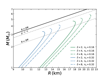
Figure 1: The M-R relations within the two-parameter model for various parameter sets of $\tilde{\epsilon}$ and $n_{s}$ in units of  MeV and $\;\text{fm}^{-3}$, respectively. The coordinate scale is logarithmic. The black hole limit $R=2M$, and the limit for central pressure to be infinite $R=9/4M$ are also shown together.

By defining $\tilde{\epsilon}=\epsilon/N_{\rm q}$ and $\bar{n}=N_{\rm q}n/n_{\rm sur}$, the simpler form of strangeon matter EOS can be derived as follows Zhang et al. (2023):

$$\frac{\rho}{n_{\rm sur}}=\frac{a}{9}\tilde{\epsilon}\left(\frac{1}{18}\bar{n}^{5}-\bar{n}^{3}\right)+m_{\rm q}\bar{n}\ ,$$ (4)

$$\frac{P}{n_{\rm sur}}=\frac{2a}{9}\tilde{\epsilon}\left(\frac{1}{9}\bar{n}^{5}-\bar{n}^{3}\right)\ ,$$

with $a=A_{6}^{2}/A_{12}$. Note that $\bar{n}=3$ at star surface where $P=0$. In the following, for convenience, we define the model containing $N_{\rm q}$, $\epsilon$, $n_{\rm sur}$ as free parameters to be the three-parameter model, and $\tilde{\epsilon}$, $n_{\rm sur}$ to be the two-parameter model, where $\tilde{\epsilon}$ means the depth per quark of the potential wall in a strangeon.

In Fig. 1, we display M-R relations of strangeon matter EOS with different sets of parameters $\tilde{\epsilon}$ and $n_{s}$ within the two-parameter model, while the three-parameter EOS are discussed in Ref. Gao et al. (2022). To better illustrate the approximately linear relationship between mass and radius at low densities, we plot the M-R relations in logarithmic space. The results indicate that it is actually the ratio of $\epsilon$ to $N_{\rm q}$ as a whole that affects the shape of M-R curve, defined as $\tilde{\epsilon}$, as shown in Eq. 4. In other words, changing the values of $\epsilon$ and $N_{\rm q}$ while keeping the $\tilde{\epsilon}$ constant does not impact the M-R relation. Increasing $n_{\rm sur}$ significantly changes the surface energy density as well as the whole range of energy densities, resulting in a softer EOS, and hence a lower maximum mass.

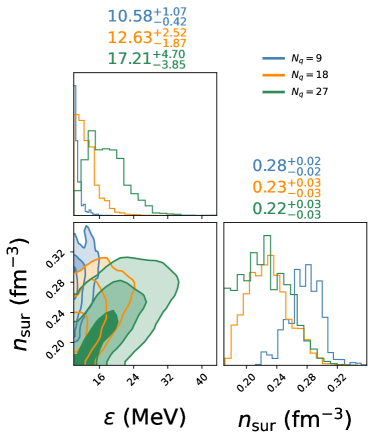
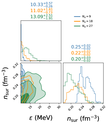
Figure 2: Left panel: The posterior distribution of the model parameters under the constraints of PSR J0030 + 0451 and PSR J0740 + 6620 at different cases of fixed $N_{\rm q}$. The contour levels in the corner plot correspond to the 68.3$\%$, 95.4$\%$, and 99.7$\%$ confidence levels, going from dark to light. Right panel: The posterior distribution of the joint analysis with PSR J0030 + 0451, PSR J0740 + 6620, and the new result measurement of PSR J0437-4715. The confidence levels are the same as in the left panel.

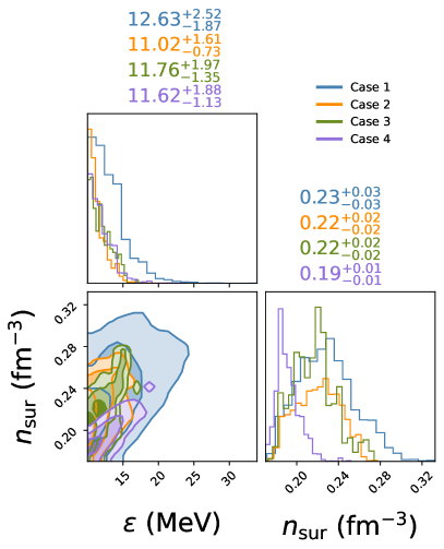
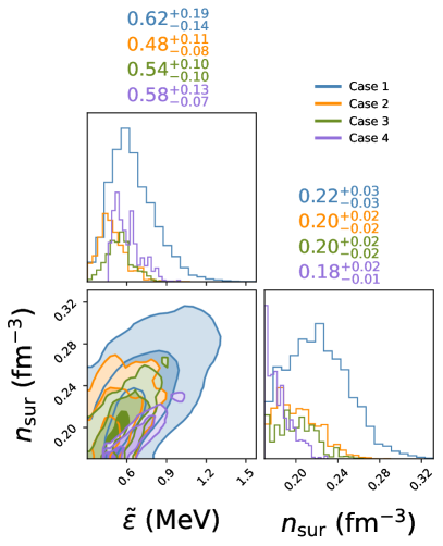
Figure 3: The posterior distributions of the three-parameter model EOS at fixed $N_{\rm q}=18$ and two-parameter model EOSs are shown in the left and right panels, respectively. Each distribution indicates the different constraints of Case 1, Case 2, Case 3, and Case 4. The contour levels in the corner plot correspond to the 68.3$\%$, 95.4$\%$, and 99.7$\%$ confidence levels, going from dark to light.

Table 1: The Bayesian evidence with and without PSR J0437-4715 for different $N_{\rm q}$. The $N_{\rm q}^{*}$ denotes the supported EOS parameter by comparing the Bayes factor with the analysis under identical observational data, which will be discussed in detail below.

Evidence	three-parameter model	$N_{\rm q}=9$	$N_{\rm q}^{*}=18$	$N_{\rm q}=24$	$N_{\rm q}=27$
logZ	without PSR J0437-4715	-34.4	-29.8	-28.9	-29.0
logZ	with PSR J0437-4715	-48.1	-36.7	-37.5	-36.0

III Constraints and Bayesian analysis

In the following, we consider the strangeon quark matter constituting the stars within two model formulation, employing Bayesian analysis to infer the posterior of strangeon matter EOS parameters, $(N_{\rm q},\epsilon,n_{\rm sur})$ or $(\tilde{\epsilon},n_{\rm sur})$, by applying multi-messenger observation constraints, and deduce the allowed M-R space of strangeon stars filtered by the observations we implied. Using this Bayesian technique, we aim to identify which $N_{\rm q}$ value aligns best with current observational constraints and to determine whether the results from three-parameter and two-parameter models are consistent under the same set of observation data.

III.1 Choice of priors for model parameters

The three-parameter model is characterized by three free parameters: $N_{\rm q}$, $\epsilon$, and $n_{\rm sur}$, which capture the unique properties of the strong interactions between strangeons as mentioned before. Although the exact values of these parameters remain uncertain, reasonable ranges can be inferred based on the current understanding of strong interactions. In this analysis, we assume the parameter $N_{\rm q}$ takes values from the set $N_{\rm q}=9$, $N_{\rm q}=18$, $N_{\rm q}=21$, $N_{\rm q}=24$, and $N_{\rm q}=27$, each a multiple of three to satisfy the requirement of color neutrality. Motivated by the evidence of the unstable H-dibaryon Bashinsky & Jaffe (1997); Wetzorke et al. (2000), which consists of six quarks in a flavor-singlet state, we consider $N_{\rm q}\geq 9$ as a minimum for the number of quarks in a strangeon. In particular, an 18-quark strangeon is called a quark-alpha Curtis Michel (1991), which is fully symmetric in spin, flavor, and color space. While the theoretical upper limit of $N_{\rm q}$ is currently unknown, we set a modestly higher upper bound of $N_{\rm q}=27$ for this analysis. As the results of the following Bayesian inference will show in Table 1, $N_{\rm q}=27$ provides an adequate prior, as the Bayes factor comparison shows no substantial improvement over the $N_{\rm q}=18$ case. Consequently, we adopt $N_{\rm q}=27$ as the upper limit in this Bayesian framework. The nucleon-nucleon scattering data indicate that the inter-nucleon potential well lies in the range of $\sim 50-120\;\text{MeV}$ for the ${}^{1}\text{S}_{0}$ (spin-singlet and s-wave) channel Stoks et al. (1994); Wiringa et al. (1995); Machleidt (2001). Since the strong interactions are not sensitive to the flavor of quarks, in this Bayesian analysis we choose $\epsilon$ spanning in the range of $10-170\;\text{MeV}$, which is needed to trap the strangeons in the potential well. The surface baryonic density $n_{\rm sur}$ should be in the same order as the nuclear saturation density, $n_{0}=0.16\;\text{fm}^{-3}$, because of the self-bound property of strangeon stars. The interactions may group the quarks more compactly compared to nuclei with the same number of quarks. Therefore, we let $n_{\rm sur}$ lie in the range of $0.17-0.36\;\text{fm}^{-3}$, which corresponds to $\sim 1n_{0}\ -2.25\ n_{0}$. Accordingly, the choice of the parameter $\tilde{\epsilon}$ is set in the range of $0.3-3.0\;\text{MeV}$ based on our prior choices for $\epsilon$ and $N_{\rm q}$ separately for the two-parameter model. These choices are clearly shown in Table 2. Due to the lack of terrestrial experimental constraints, all parameters are investigated with uniform contributions in this work.

III.2 Inference framework

According to the Bayes’ theorem, the posterior distribution of a set of model parameters $\theta$ given the observational data set $\bm{d}$ for a model $\mathcal{M}$ can be

$$p\left(\bm{\theta}\mid\bm{d},\mathcal{M}\right)=\frac{p\left(\bm{d}\mid\bm{\theta},\mathcal{M}\right)p\left(\bm{\theta}\mid\mathcal{M}\right)}{p(\bm{d}\mid\mathcal{M})}\ ,$$ (5)

where $p\left(\bm{\theta}\mid\mathcal{M}\right)$ is the prior probability of the parameter set $\theta$. $p\left(\bm{d}\mid\bm{\theta},\mathcal{M}\right)$ is the likelihood function of the data given the model, and $p(\bm{d}\mid\mathcal{M})$ is known as evidence for the model. For a given data set $p(\bm{d}\mid\mathcal{M})$ is a constant and can be treated as a normalization factor. Since different central energy densities correspond to different masses and radii, for the present analysis, we need the parameter $\varepsilon_{\rm c}$ to perform the Bayesian analysis. Hence, the posterior distributions of the EOS model parameters $\theta$ and center energy densities $\varepsilon_{\rm c}$ can be written as:

$$p(\bm{\theta},\varepsilon_{\rm c}\mid\bm{d},\mathcal{M})\propto p(\bm{\theta}\mid\mathcal{M})p(\varepsilon_{\rm c}\mid\bm{\theta},\mathcal{M})p(\bm{d}\mid\bm{\theta},\mathcal{M})\ ,$$ (6)

where $p(\bm{\theta}\mid\mathcal{M})$ and $p(\varepsilon_{\rm c}\mid\bm{\theta},\mathcal{M})$ are the prior distributions of $\theta$ and $\varepsilon_{\rm c}$ respectively. $p(\bm{d}\mid\bm{\theta},\mathcal{M})$ is the nuisance-marginalized likelihood function (see Refs. Raaijmakers et al. (2021); Huang et al. (2024) for the detail discussions for the definition). The astrophysical inputs as the likelihood for our inference are explained as follows.

III.2.1 Constraints from NICER data

We consider the masses and radii inferred from the NICER data, by Riley et al. 2019ApJ…887L..21R ; 2021ApJ…918L..27R ; Vinciguerra et al. (2024), for PSR J0030 + 0451 we use the result from 2019ApJ…887L..21R ($M=1.34^{+0.15}_{-0.16}\,M_{\odot}$ and $R=12.71^{+1.14}_{-1.19}\rm km$) and the heavy pulsar PSR J0740 + 6620 ($M=2.072^{+0.067}_{-0.066}\,M_{\odot}$ and $R=12.39^{+1.30}_{-0.98}\rm km$) by X-ray pulse profile modeling of NICER data. Here, we also consider the impact of the new result on the mass measurement for the $\sim 1.4\,M_{\odot}$ pulsar PSR J0437-4715 Choudhury et al. (2024); Rutherford et al. (2024). Using a mass prior from radio timing Reardon et al. (2024) people reported a mass of $M=1.418\pm 0.037\,M_{\odot}$ and a radius of $R=11.36_{-0.63}^{+0.95}\mathrm{~{}km}$ (68% credible intervals) for PSR J0437-4715.

Given that all of the measurements are independent, by equating the nuisance-marginalized likelihoods to the nuisance-marginalized posterior distributions Raaijmakers et al. (2021); Huang et al. (2024), we can rewrite the likelihood as follows:

$$p(\bm{\theta},\varepsilon_{\rm c}\mid\bm{d},\mathcal{M})\propto p(\bm{\theta}\mid\mathcal{M})p(\varepsilon_{\rm c}\mid\bm{\theta},\mathcal{M})$$ (7)

$$\quad\times\prod_{j}p\left(\bm{M}_{j},R_{j}\mid d_{\mathrm{NICER},\mathrm{j}}\right)\ ,$$

with $j$ representing the different measurements of masses and radii inferred from the NICER data.

Table 2: The most probable intervals of the EOS parameters (68.3 $\%$ confidence level) as well as the strangeon star properties ($90\%$ confidence level) in three-parameter and two-parameter models constrained by Case 1 (PSR J0030+0451 $\&$ PSR J0740+6620), Case 2 (PSR J0030+0451 $\&$ PSR J0740+6620 $\&$ PSR J0437-4715), Case 3 (PSR J0030+0451 $\&$ PSR J0740+6620 $\&$ PSR J0437-4715 $\&$ GW170817, and Case 4 (PSR J0030+0451 $\&$ PSR J0740+6620 $\&$ PSR J0437-4715 $\&$ GW170817 $\&$ GW190814), respectively. $\mathcal{U}$ means Uniform (Flat) distribution. $M_{\rm TOV}$ is the maximum mass. $R_{\rm 1.4}$ and $R_{2.1}$ are the radii of $1.4\,M_{\odot}$ and $2.1\,M_{\odot}$ stars, espectively.

three-parameter model ($N_{\rm q}=18$)	$\mathrm{Prior}$	Case 1	Case 2	Case 3	Case 4
$\epsilon~{}(\rm MeV)$	$\mathcal{U}(10,170)$	$12.63^{+2.52}_{-1.87}$	$11.02^{+1.61}_{-0.73}$	$11.76^{+1.97}_{-1.35}$	$11.62^{+1.88}_{-1.13}$
[$\epsilon/N_{\rm q}~{}(\rm MeV)$		$0.70^{+0.14}_{-0.10}$	$0.61^{+0.09}_{-0.04}$	$0.65^{+0.11}_{-0.08}$	$0.65^{+0.10}_{-0.06}$]
$n_{\rm sur}~{}(\rm fm^{-3})$	$\mathcal{U}(0.17,0.36)$	$0.23^{+0.03}_{-0.03}$	$0.22^{+0.02}_{-0.02}$	$0.22^{+0.02}_{-0.02}$	$0.19^{+0.01}_{-0.01}$
$R_{1.4}~{}(\rm km)$		$11.32^{+0.76}_{-0.61}$	$11.33^{+0.66}_{-0.48}$	$11.47^{+0.60}_{-0.51}$	$12.04^{+0.27}_{-0.31}$
$R_{2.0}~{}(\rm km)$		$12.59^{+0.71}_{-0.81}$	$12.56^{+0.72}_{-0.62}$	$12.62^{+0.69}_{-0.60}$	$13.28^{+0.24}_{-0.35}$
$M_{\rm TOV}(M_{\odot})$		$3.51^{+0.22}_{-0.10}$	$3.48^{+0.21}_{-0.10}$	$3.51^{+0.18}_{-0.09}$	$3.58^{+0.16}_{-0.12}$
two-parameter model	$\mathrm{Prior}$	Case 1	Case 2	Case 3	Case 4
$\tilde{\epsilon}$	$\mathcal{U}(0.3,3)$	$0.62^{+0.19}_{-0.14}$	$0.48^{+0.11}_{-0.08}$	$0.54^{+0.10}_{-0.10}$	$0.61^{+0.09}_{-0.07}$
$n_{\rm sur}~{}(\rm fm^{-3})$	$\mathcal{U}(0.17,0.36)$	$0.22^{+0.03}_{-0.03}$	$0.20^{+0.02}_{-0.02}$	$0.20^{+0.02}_{-0.02}$	$0.18^{+0.01}_{-0.01}$
$R_{1.4}~{}(\rm km)$		$11.43^{+0.71}_{-0.73}$	$11.65^{+0.48}_{-0.62}$	$11.69^{+0.58}_{-0.51}$	$12.16^{+0.26}_{-0.31}$
$R_{2.0}~{}(\rm km)$		$12.51^{+0.79}_{-0.86}$	$12.66^{+0.64}_{-0.66}$	$12.95^{+0.53}_{-0.71}$	$13.38^{+0.27}_{-0.41}$
$M_{\rm TOV}(M_{\odot})$		$3.52^{+0.17}_{-0.08}$	$3.49^{+0.19}_{-0.11}$	$3.51^{+0.17}_{-0.12}$	$3.65^{+0.18}_{-0.16}$

III.2.2 Constraints from gravitational wave events

The tidal deformability inferred from gravitational wave detection of binary neutron star mergers have also led to a steady improvement in our understanding of the dense matter EOS. Here, we consider the constraints from the gravitational wave events GW170817 2017PhRvL.119p1101A ; 2018PhRvL.121p1101A and GW190814 Abbott et al. (2020) reported by the LIGO Scientific Collaboration, and study the mass-gap secondary object ($M=2.59^{+0.08}_{-0.09}\,M_{\odot}$) in GW190814 potentially being a strangeon star.

When treating the GW events, we fix the chirp mass $M_{\mathrm{c}}=$ $\left(M_{1}M_{2}\right)^{3/5}/\left(M_{1}+M_{2}\right)^{1/5}$ to the median value $M_{\mathrm{cl}}=1.186\mathrm{M}_{\odot}$ for GW170817. Ref. Raaijmakers et al. (2021) has shown that the small bandwidth of the chirp masses has almost no significant influence on the posterior distribution, contributing less than the sampling noise. We therefore fix the chirp mass, which is also beneficial in reducing the dimensionality of the parameter space and hence the computational cost. To speed up convergence of our inference process, we transform the GW posterior distributions to include the two tidal deformabilities, chirp mass and mass ratio $q$, simultaneously reweighing such that the prior distribution on these parameters is uniform. The posterior then becomes

$$p(\bm{\theta},\varepsilon_{\rm c}\mid\bm{d},\mathcal{M})\propto p(\bm{\theta}\mid\mathcal{M})p(\varepsilon_{\rm c}\mid\bm{\theta},\mathcal{M})$$ (8)

$$\times\prod_{i}p\left(\Lambda_{1,i},\Lambda_{2,i},q_{i}\mid\mathcal{M}_{\rm c},\bm{d}_{\mathrm{GW},\mathrm{i}}\left(,\bm{d}_{\mathrm{EM},\mathrm{i}}\right)\right)$$

$$\times\prod_{j}p\left(M_{j},R_{j}\mid\bm{d}_{\mathrm{NICER},\mathrm{j}}\right)\ ,$$

where $\Lambda_{2,i}=\Lambda_{2,i}\left(\bm{\theta};q_{i}\right)$ is the tidal deformability, with the $i$th indicating the individual-event GW likelihood marginalized over all binary parameters. We follow the same convention as demonstrated in Ref. 2018PhRvL.121p1101A and define $M_{1}>M_{2}$, since the gravitational wave likelihood function is degenerate under the exchange of the binary components.

All the inferences in this work employs the CompactObject packageHuang et al. (2024), developed by the author and detailed in the Zenodo repository Huang et al. (2023). CompactObject is the inaugural open-source package that is extensively documented and offers comprehensive functionalities for applying Bayesian methods to constrain the EOS of neutron stars. It supports various EOS models, such as relativistic mean field (RMF) and polytropes, and has been utilized in other studies like Huang et al. (2024); Huang_2024 . For the Bayesian inference, we used the UltraNest package Buchner (2021), specifically employing its slice sampler, which is available at Github. We chose to use 50,000 live points for each inference to establish a baseline for comparing Bayes evidence, ensuring efficient and consistent high-dimensional sampling and convergence speeds.

IV Results and discussions

IV.1 three-parameters case

In Fig. 2, we present the posterior distribution of EOS parameters in three-parameter model, where we show the typical cases of $N_{\rm q}=9$, $N_{\rm q}=18$, and $N_{\rm q}=27$ in each panel. The left panel depicts the joint analysis of PSR J0030+0451 and PSR J0740+6620, while the right panel includes an additional observation data incorporating PSR J0437-4715. The contour levels in each corner plot indicate the 68.3%, 95.4%, and 99.7% confidence regions, shaded from dark to light, respectively. Comparing the posterior parameter space across different choices of $N_{\rm q}$, we could explore the optimal choice for this quantity. Our results demonstrate that increasing $N_{\rm q}$ in these joint Bayesian analyses favors larger values of $\epsilon$ and smaller values of $n_{\rm sur}$. This trend aligns with our theoretical understanding: as $N_{\rm q}$ increases, the EOS softens, leading to a deeper potential $\epsilon$ and a reduced surface baryon density $n_{\rm sur}$ to counteract the additional softening by enhancing the repulsive interactions. Comparing the results across two plots under the same $N_{\rm q}$, including PSR J0437-4715 results in a smaller $\epsilon$ and correspondingly smaller $n_{\rm sur}$. With other parameters unchanged, a smaller $\epsilon$ results in a softer EOS, and a smaller $n_{\rm sur}$ corresponds to a stiffer EOS. Therefore, the inclusion of this new observation has a mixed effect on the EOS parameters.

Bayes factors, which are defined by $\rm log\ K=log(Z_{1}/Z_{2})$ where $Z$ is the Bayesian evidence, are used to compare the capability of different models of 1 and 2 to reconstruct the injected EOS. Per the standards in Ref. kass et al. (1995), a model is substantially preferred if its Bayes factor is above 3.2, strongly preferred when the factor exceeds 10, and decisive with a Bayes factor greater than 100. Table. 1 presents the Bayesian evidence for several selected cases with varying $N_{\rm q}$ under the finite $N_{\rm q}$ value assumption motivated by the strangeon matter hypothesis. Under the constraints of PSR J0030+0451 and PSR J0740+6620, the generally growing evidence indicates that the data predominantly favor the large $N_{\rm q}$ model. Specifically, when comparing the $N_{\rm q}=18$ model to the $N_{\rm q}=9$ model, the analysis relatively supports the EOS model with $N_{\rm q}=18$ as indicated by a Bayes factor of $\mathrm{K}=(Z_{1}/Z_{2})=99.5$, which signifies decisive evidence in favor of $N_{\rm q}=18$. When additional data from PSR J0437-4715 are incorporated, the preference for $N_{\rm q}=18$ is further strengthened, with an exceptionally large Bayes factor of $\mathrm{K}=80,821$. This statistical evidence favors the fully symmetric configuration in spin, flavor, and color space for $N_{\rm q}=18$. Continuing to increase $N_{\rm q}$ could result in a slight improvement in the log evidence, from $-29.8$ to $-28.9$, when $N_{\rm q}$ is raised to $24$ under the consideration of only PSR J0030+0451 and PSR J0740+6620. However, this improvement is minimal, making it reasonable to truncate the indefinite increase of $N_{\rm q}$ at a value of $18$. Furthermore, when PSR J0437-4715 is included, the evidence exhibits a local maximum at $N_{\rm q}=18$ as $N_{\rm q}$ increases. Since models with $N_{\rm q}=9$ and $N_{\rm q}=24$ demonstrate lower evidence values, this observation further supports our decision to fix $N_{\rm q}$ at $18$.

Thus in the subsequent analyses, we fixed the number of quarks in a strangeon to $N_{\rm q}=18$, reflecting the strong support from previous results. Fig. 3 displays the marginalized posterior distribution functions for the EOS parameters, derived from four distinct cases of joint analyses under various astronomical constraints, described as follows:

• Case 1: The joint analysis of PSR J0030+0451 ($M=1.34_{-0.16}^{+0.15}\mathrm{M}_{\odot},R=12.71_{-1.19}^{+1.14}\mathrm{~{}km}$) and the heavy pulsar PSR J0740+6620 ($M=2.07\pm 0.07\mathrm{M}_{\odot},R=12.39_{-0.98}^{+1.30}\mathrm{~{}km}$).

• Case 2: Joint analysis including PSR J0030+0451, PSR J0740+6620, and PSR J0437-4715 ($\sim 1.418,M_{\odot},\sim 11.36$ km).

• Case 3: Analysis under the combined constraints from PSR J0030+0451, PSR J0740+6620, PSR J0437-4715, and the GW170817 gravitational wave event.

• Case 4: The most comprehensive case, including data from PSR J0030+0451, PSR J0740+6620, PSR J0437-4715, along with gravitational wave observations from GW170817, and incorporating the mass measurement of GW190814’s secondary component, $2.59_{-0.09}^{+0.08}M_{\odot}$ (at the $90\%$ confidence level) as a lower bound on the maximum mass.

Table 2 presents posterior values of the EOS parameters, along with their 68.3% confidence intervals, and the most probable intervals of the starangeon star properties with 90% confidence levels. The preferred parameter estimates for the Case 1 analysis are $\epsilon=12.63^{+2.52}_{-1.87}\;\text{MeV}$ and $n_{\rm sur}=0.23^{+0.03}_{-0.03}\;\text{fm}^{-3}$. Incorporating the constraints from GW170817 shows a clear trend toward a slightly stiffer EOS by comparing the results from Case 2 and Case 3, as evidenced by a increase in $\epsilon$ from $11.02^{+1.61}_{-0.73}\;\text{MeV}$ to $11.76^{+1.97}_{-1.35}\;\text{MeV}$, while the posterior distributions for $n_{\rm sur}$ in Case 2 is the same as Case 3’s results. Although including PSR J0437-4715 in Case 2 analysis further reduces $\epsilon$ compared with Case 1, thereby softening the EOS, it simultaneously introduces a stiffening effect by decreasing the surface density $n_{\rm sur}$. The parameter $\epsilon$ exhibits slight differences in its posterior distribution between these cases, reflecting subtle variations in the inferred EOS properties as additional constraints are considered. Interestingly, once $N_{\rm q}$ is fixed at 18, the normalized $\tilde{\epsilon}$ can be calculated. As the number of observations increases, this ratio remains approximately constant, around 0.65. Surprisingly, the inclusion of GW190814 does not further increase or decrease this value in Case 4 compared to previous cases in three-parameter EOS model. The secondary object of GW190814 is classified as a mass-gap object, which typically necessitates a much stiffer EOS. However, the strangeon EOS employed in this study is inherently stiff, allowing it to easily satisfy the high-mass observational constraints. This demonstrates a significant advantage of the strangeon EOS, as it can simultaneously satisfy the very high mass criteria while adequately explaining all other observations. Additionally, the reason why including this mass-gap object did not substantially refine the posterior is that this object only provides mass information without accompanying radius or tidal deformability data. Consequently, this results in looser constraints on the strangeon matter EOS.

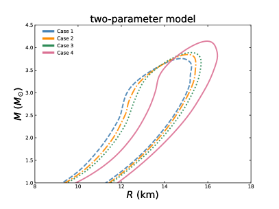
Figure 4: The M-R posterior distributions at $90\%$ confidence level resulting from the three-parameter and two-parameter models.

IV.2 Comparison with two-parameter case

As we mentioned before, the free parameters for strangeon matter EOS can be reduced to two parameters by defining $\tilde{\epsilon}=\epsilon/N_{\rm q}$ and $\bar{n}=N_{\rm q}n/n_{\rm sur}$. The influence of $\epsilon$ and $N_{\rm q}$ on mass and radius is concurrent, thus only changing $\tilde{\epsilon}$ can produce a different M-R curve, that is to say, the parameters $\tilde{\epsilon}$ and $n_{\rm sur}$ fully determine the EOS stiffness and the overall shape. An increase in the average potential depth per strangeon, $\tilde{\epsilon}$, and a reduction in surface baryon number density, $n_{\rm sur}$, resulting in a stiffer EOS due to the enlarged phenomenologically repulsive force. In this section, we aim to test the results between these models with different degrees of freedom EOS parameters.

Like three-parameter model, the right panel of Fig. 3 displays the posterior distribution for the two-parameter EOS model, $\tilde{\epsilon}$ and $n_{\rm sur}$, while Table 2 provides the posteriors of the EOS parameters and their 68.3$\%$ confidence range. As illustrated in Fig. 3, a heavy star of mass $2.1\,M_{\odot}$ and a $1.4\,M_{\odot}$ star require: $\tilde{\epsilon}=0.62^{+0.19}_{-0.14}\;\text{MeV}$, $n_{\rm sur}=0.22^{+0.03}_{-0.03}\;\text{fm}^{-3}$. When considering additional constraints from PSR J0437-4715, the results show a lower value for both $\tilde{\epsilon}=0.48^{+0.11}_{-0.08}\;\text{MeV}$ and $n_{\rm sur}=0.20^{+0.02}_{-0.02}$. Therefore, it is hard to say the direct influence of this constraint on the EOS property, since a lower $\tilde{\epsilon}$ leads to a softer EOS while a smaller $n_{\rm sur}$ results in a stiffer EOS, which is consistent with the results of the Bayesian analysis for the three-parameter model under the same constraints. However, the gravitational event GW170817 has a straightforward influence on $\tilde{\epsilon}$ by comparison of Case 2 and Case 3. GW170817 requires a slightly stiffer EOS to accommodate a slightly larger radius than PSR J0437-4715. Previous studies have suggested that the secondary object in GW190814 could potentially be a quark star, considering the interacting quark matter Zhang & Mann (2021); Bombaci et al. (2021); Cao et al. (2022). Given the inherently stiff nature of the strangeon matter EOS, we also consider the constraints of GW190814. The results obviously indicate that a stiffer EOS with larger $\tilde{\epsilon}=0.61^{+0.09}_{-0.07}\;\text{MeV}$ and smaller $n_{\rm sur}=0.18^{+0.01}_{-0.01}\;\text{fm}^{-3}$ is required to support this observation.

IV.3 The M-R posteriors and maximum mass of strangeon stars

Mapping the EOS posteriors to M-R space facilitates the understanding of how observational constraints influence the EOS and delineates the allowable regions in M-R space based on specific EOS models informed by various sets of observational data. We show in Fig. 4 the M-R contours corresponding to the posterior distributions of the strangeon star EOSs. Every point in the EOS parameter space is uniquely correlated to a point in EOS posterior parameter space. Then by varying central density, EOS points can be mapped to the M-R plane through deriving the Tolman-Oppenheimer-Volkoff (TOV) equations.

Fig. 4 demonstrates that incorporating additional astronomical observations in the Bayesian analysis refines the M-R space for both three-parameter and two-parameter models, yielding more constrained M-R relations. The stiffness of the strangeon matter EOS leads to the dominant role of the PSR J0740+6620 compared to the results of Bayesian analyses in Cases 1, 2, and 3, with the addition of further observational constraints only slightly changing the shape of the M-R curve. In particular, the inclusion of the GW190814 constraint excludes excessively soft EOSs, thus supporting the existence of superheavy compact stars around $\sim 4.0\,M_{\odot}$. This suggests that strangeon matter could feasibly support the structure of massive compact objects that may be observed in the future. One can also evaluate the star’s important properties as illustrated in Table 2 in detail. For example, the radius of a $1.4\,M_{\odot}$ star is constrained to $11.47^{+0.60}_{-0.51}\rm km$ ($11.69^{+0.58}_{-0.51}$) in the three-parameter (two-parameter) model for Case 3. Similarly, the radius for a $2.0\,M_{\odot}$ star is approximately $1\rm km$ larger than for a $1.4\,M_{\odot}$ star, with values of $12.62^{+0.69}_{-0.60}\rm km$ ($12.95^{+0.53}_{-0.71}\rm km$) for the three-parameter (two-parameter) model, which is in line with our expectations, since the difference between the measured radii of J0437-4715 and J0740+6620 is about 1 km. In these analyses, both three-parameter and two-parameter EOSs can easily favor the superheavy compact objects above $\sim 2.6\,M_{\odot}$. The maximum mass of strangeon stars can be $\sim 3.8\,M_{\odot}$. Including GW190814 changes the results to favor more massive compact stars.

V Summary

In conclusion, we use Bayesian analysis to explore the parameter space of the EOSs for strangeon matter constrained by recent astronomical observations. In particular, This analysis includes the new mass and radius measurements for PSR J0437-4715 and the secondary component of the GW190814 gravitational wave event, a mass-gap object. Due to the limited constraints on strangeon matter from terrestrial experiments, astronomical observations play a crucial role in guiding the parameter space for this exotic matter. Our study also provides a comparative analysis of the posterior EOS parameter spaces derived from two different models: a three-parameter model and a two-parameter model. Both models are evaluated under identical observational constraints, allowing us to assess how each model adapts to the data. Despite differences in their theoretical formulations, these two models are largely consistent in predicting a stiff EOS. They can easily reproduce the mass-gap object observed in GW190814 while still satisfying all current observations. This consistency aligns with the inherently stiff nature of the strangeon EOS model and demonstrates the advantage of this EOS model in explaining the observational data. The results suggest that current astronomical observations support $18$ quarks per strangeon, $N_{\rm q}=18$, indicating a preference for this quark configuration in the strangeon-matter model.

When fixing $N_{\rm q}=18$, Bayesian analyses of both the two- and three-parameter models yield a consistent ratio of $\epsilon/N_{\rm q}$ around 0.6. Considering observational constraints from PSR J0030+0451, PSR J0740+6620, PSR J0437-4715, and GW170817, the inferred radius for a $1.4\,M_{\odot}$ star is $11.47^{+0.60}_{-0.51}\rm km$ in the three-parameter model and slightly increased to $11.69^{+0.58}_{-0.51}\rm km$ in the two-parameter model. For a massive $2.0\,M_{\odot}$ star, the corresponding radii are $12.62^{+0.69}_{-0.60}\rm km$ and $12.95^{+0.53}_{-0.71}\rm km$, respectively. By incorporating the mass measurement of GW190814’s secondary component, $2.59_{-0.09}^{+0.08}M_{\odot}$ (at the $90\%$ confidence level), as a lower bound on the maximum mass, the upper boundary of $\tilde{\epsilon}$ is increased from $0.64\;\text{MeV}$ to $0.70\;\text{MeV}$ in the two-parameter model at the $68.3\%$ confidence level. Due to the stiff nature of strangeon matter EOS, the change is slight. In addition, we find that, for a $2.6M_{\odot}$ star like GW190814’s secondary component, the radius is $14.33^{+0.29}_{-0.45}\rm km$. Future measurements of such massive compact objects could provide further insights into the dense matter EOS and the internal nature of compact objects.

Our results could be relevant to a hot topic of multiquark states Chen et al. (2016); Guo et al. (2018). The state of strongly interacting matter remains certainly a fundamental question directly related to the physics of compact stars. Resolving the mystery of dense matter has motivated extensive efforts, leading to several proposals for alternatives of neutron matter in the interior of compact stars, including strange quark matter Bodmer (1971); Witten (1984), two-flavor quark matter Holdom et al. (2018); Ren & Zhang (2020); Zhang (2020); Zhang & Mann (2021), quarkyonic matter with baryonic exci- tations near the Fermi surface McLerran & Pisarski (2007); Herbst et al. (2011); Shao et al. (2011); Kojo (2012), and strangeon matter with quark condensation in position space Xu (2003); Xu et al. (2006); Peng & Xu (2008); Lai & Xu (2009); Liu et al. (2012); Zhou et al. (2014); Lai & Xu (2016); Lai et al. (2018, 2019, 2021); Gao et al. (2022); Miao et al. (2022); Zhang et al. (2023, 2023), as an incomplete list of examples. Among those efforts, the strangeon as a kind of stable bound state could be natural in QCD, which might attract particular interest in future study of multi-quark states. Our Bayesian analysis strongly supports the scenario in which a strangeon forms a stable bound state with $N_{\rm q}=18$, exhibiting symmetry in color, flavor, and spin spaces. Investigating the interactions between strangeons provides valuable insights into strongly interacting matter and the EOS of dense matter. Nevertheless, advancing our understanding of strangeon matter further will rely on forthcoming experimental and observational developments, which are expected to provide crucial perspectives on its properties and its role in the composition of compact stars.