On a local solvability of the contact Muskat problem

Abstract.

In the paper, we discuss the two-dimensional contact Muskat problem with zero surface tension on a free boundary. The initial shape of the unknown interface is a smooth simple curve which forms acute corners $\delta_{0}$ and $\delta_{1}$ with fixed boundaries. Under suitable assumptions on the given data, the one-to-one local classical solvability of this problem is proved. We also describe the sufficient conditions on the data in the model which provide the existence of the ”waiting time” phenomenon.

1. Introduction

The Muskat problem proposed by Morris Muskat [29] in 1934 is a classical model describing the viscous displacement in a two-phase fluid system occupied a two-dimensional porous medium. As noted in [29, 30], this problem describes the encroachment of water into oil sand and deals with the secondary phase of the oil recovery process, where water injection is utilized to enlarge the pressure in the oil reservoir and to move the oil to the production well. The fluids’ motion is subjected by the experimental Darcy law. The boundary between the two liquid regions is an unknown needing to be searched. This moving (unknown) interface is usually called a free boundary and, accordingly, the Muskat problem is a free boundary problem.

For the last 70 years, thanks to various applications in hydrodynamics, chemistry and oil industry, the Muskat model and the associated problems have attracted a wide scientific interests among the mathematical, engineering and chemical community. As mentioned in [20], there is an enormous literature on these problems in various geometries and physical settings, where analytical and numerical investigations are carried out via various techniques and approaches.

In this paper, we focus on the two-dimensional contact Muskat problem in the case of the zero surface tension (ZST) of the moving interface. Let $\Omega\subset\mathbb{R}^{2}$ be a bounded domain with a smooth boundary $\partial\Omega\in\mathcal{C}^{2+\beta},$ $\beta\in(0,1).$ For each $\tau\in[0,T],$ a simple curve $\Gamma(\tau)\subseteq\bar{\Omega}$ splits the domain $\Omega$ onto two sub-domains $\Omega_{1}(\tau)$ and $\Omega_{2}(\tau)$ such that

$$\Omega=\Omega_{1}(\tau)\cup\Omega_{2}(\tau)\cup\Gamma(\tau),\quad\Omega_{1}(\tau)\cap\Omega_{2}(\tau)=\emptyset,\quad\partial\Omega_{1}(\tau)\cap\partial\Omega_{2}(\tau)=\Gamma(\tau)$$

and, besides, $\Gamma(\tau)$ intersects with $\partial\Omega$ at two corner points $\mathbf{A}_{0}$ and $\mathbf{A}_{1}$, i.e.

$$\partial\Omega\cap\Gamma(\tau)=\{\mathbf{A}_{0},\mathbf{A}_{1}\}$$

(see Figure 1 for geometric settings).

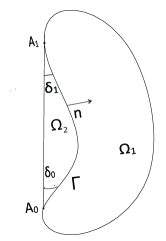
(a)

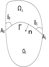
(b)

Figure 1. Typical configurations of the initial domains $\Omega_{i}$ and $\Gamma$.

For fixed positive quantities $T,$ $k_{1}$ and $k_{2},$ $k_{1}\neq k_{2}$, we look for unknown fluid pressures $\mathrm{P}_{1}=\mathrm{P}_{1}(y_{1},y_{2},\tau),$ $\mathrm{P}_{2}=\mathrm{P}_{2}(y_{1},y_{2},\tau)$ in the corresponding liquid domains $\Omega_{1}(\tau)$ and $\Omega_{2}(\tau)$, and the unknown interface $\Gamma(\tau)$ satisfying the system

$$\begin{cases}\Delta_{y}\mathrm{P}_{i}=0\quad\text{in}\quad\Omega_{i}(\tau),\quad\tau\in(0,T),\quad i=1,2,\\ \mathrm{P}_{1}-\mathrm{P}_{2}=0\quad\text{on}\quad\Gamma(\tau),\quad\tau\in[0,T],\\ V_{n}=-k_{1}\frac{\partial\mathrm{P}_{1}}{\partial n_{\tau}}=-k_{2}\frac{\partial\mathrm{P}_{2}}{\partial n_{\tau}}\quad\text{on}\quad\Gamma(\tau),\quad\tau\in[0,T],\\ \mathrm{P}_{1}=\mathrm{p}_{1}(y)\quad\text{on}\quad\partial\Omega_{1}(\tau)\backslash\Gamma(\tau),\quad\tau\in[0,T],\\ \mathrm{P}_{2}=\mathrm{p}_{2}(y)\quad\text{on}\quad\partial\Omega_{2}(\tau)\backslash\Gamma(\tau),\quad\tau\in[0,T],\\ \Gamma(0)=\Gamma\quad\text{is given}.\end{cases}$$ (1.1)

Here $\Delta_{y}=\frac{\partial^{2}}{\partial y_{1}^{2}}+\frac{\partial^{2}}{\partial y_{2}^{2}}$, $n_{\tau}$ denotes the outward normal to $\Gamma(\tau)$ directed in $\Omega_{1}(\tau)$, the functions $\mathrm{p}_{1}$ and $\mathrm{p}_{2}$ are prescribed. Finally, the symbol $V_{n}$ stands for the velocity of the free boundary $\Gamma(\tau)$ in the direction of $n_{\tau}$.

It is apparent that the mathematical statement of the contactless Muskat problem is the similar to (1.1) where $\Gamma(\tau)$ is assumed to be a simple smooth or nonsmooth closed curve separating $\Omega$ into two corresponding subdomains. It is worth noting that the accounting surface tension of the interface $\Gamma(\tau)$ in the $n$-dimensional Muskat model is achieved via introducing the term $\sigma\mathrm{H}_{\Gamma(\tau)}$ in the right-hand side of the first condition on $\Gamma(\tau)$ in (1.1), that is

$$\mathrm{P}_{1}-\mathrm{P}_{2}=\sigma\mathrm{H}_{\Gamma(\tau)}\quad\text{on}\quad\Gamma(\tau),\,\tau\in[0,T],$$

where $\sigma$ is the coefficient of the surface tension, while $\mathrm{H}_{\Gamma(\tau)}$ denotes the $(n-1)$-fold mean curvature.

The study of the (contactless) Muskat problem has a long history. We do not provide, here, a complete survey on the outcomes related to this and associated problems, but rather present some of them. The first result on the classical solvability on a $2$-dim. domain in the case of the nonzero surface tension (NZST) was established in [24]. The stability of a circular steady-state in the unbounded domain is discussed in [19]. In particular, the authors state that the equilibrium is not asymptotically stable. The one-valued classical solvability of the Muskat problem in a horizontally periodic geometry is proved in [15] in the case of presence of the surface tension and of gravity. Besides, the authors obtain the exponential stability of certain flat equilibria and, utilizing the bifurcation theory, they find finger shaped (unstable) steady-states. We refer [15, 16, 18], where employing the abstract parabolic theory, the authors refine and extend the aforementioned results. In [26], the well-posedness of the Muskat problem with positive $\sigma$ including the criterion of the global solvability is discussed in the subcritical Sobolev spaces. In fine, we quote [5], where the existence of the waiting time in the two-dimensional Muskat problem with NZST stated in domains with singular boundaries is established. We recall that the waiting time phenomenon in the Muskat model and the associated problems means the existence of a positive time $T^{*}$, such that the geometry of the free boundary at singularities preserves and/or these singular points do not move for each $t\in[0,T^{*}]$.

Coming to the Muskat problem in the ZST case, it is well-known, that this model can be ill-posed. Namely, this option occurs if the Rayleigh-Taylor condition is not fulfilled. Other words, it is happen if either the more viscous liquid displaces the less viscous fluid, or the heavier liquid is located above the lighter one (see for details [3]). In [39], the first local classical solvability was established by Newtonian iteration technique. We refer works [8, 9, 11, 12, 14, 13, 17, 27, 33, 38, 40], where various aspects associated with the equivalence of statement, local and global well-posedness, regularity, breakdown of smoothness, finite time turning and stability shifting are discussed with employing energy approach, methods of complex analysis, the Cauchy-Kowalewski theorem, fixed-point arguments, the abstract well-posedness result based on continuous maximal regularity. The evolution of the singularities being located on the initial shape of the moving boundaries are described in [2, 6, 20, 21]. For further acquaintance with results, we refer readers to the papers [9, 27, 28] and monographs [32], where a brief overview (including a historic survey) of the Muskat problem is done.

As for the study of the contact free boundary problems to Laplace equations similar to (1.1), we mention [4, 31, 36], where the contact Hele-Shaw free boundary problems (sometimes calling as the one-phase Muskat problem) with and without surface tension are discussed. Namely, in these works, the unknown interface and the fixed boundaries form either acute angles [4, 36] or the right angle [31]. Besides, the authors proved the local classical solvability of these problem and establish the existence of the waiting time under certain assumptions on the given data in these models.

To the author’s best knowledge, there are no works in the literature addressing the study of the evolution of the moving interface in the contact Muskat problem (1.1). The aim of this article is to fill this gap, providing a (locally in time) well-posedness result along with the regularity of solution in the weighted Hölder spaces. Moreover, under certain assumptions on the initial geometry of the domains and the given functions and parameters in the model, we analyze the existence of the waiting time phenomenon in (1.1).

In the course of this investigation, we exploit the following technique including the $4^{th}$ main steps. In the first stage, introducing the special type vector field and utilizing the Hanzawa-type transformation (accounting the nonsmooth boundaries of $\Omega_{i}(0)$), we reduce problem (1.1) to a nonlinear problem defined in fixed domains $\Omega_{i}(0)\times(0,T),$ $i=1,2$. The we linearize this nonlinear problem on the initial data $\mathrm{P}_{i}(y,0)$ and on the special constructed function $\rho(y,t)$ related with the initial shape of the interface $\Gamma.$ After that, we solve the nonclassical linear interface problem to Poisson equations stated in $\Omega_{i}(0)\times(0,T)$ having nonsmooth boundaries $\partial\Omega_{i}(0)\times(0,T)$. The nonclassical character of this problem is related with a dynamic boundary condition as the one of the transmission conditions on $\Gamma\times[0,T]$. To prove the one-valued classical solvability of this linear problem in the weighted Hölder classes (which is more natural in the case of singular boundaries), we collect the continuation approach with studying the corresponding model problems providing the a priori estimates. In fine, coming to the nonlinear problem and utilizing contraction mapping principle, we establish the local classical one-to-one solvability of (1.1). Further, appealing to the properties of the weighted Hölder classes and employing the classical solvability of the contact Muskat problem, we arrive at the existence of the waiting time phenomenon under assumptions on the given data providing the local well-posedness. The later, in particular, means that

$$\delta_{0},\delta_{1}\in(0,\pi/4),\quad 0<k_{2}<k_{1}\quad\frac{\partial P_{i}(y,0)}{\partial n_{\tau}}|_{\Gamma}<0,\quad i=1,2.$$

Outline of the Paper

The paper is organized as follows. In Section 2, we introduce the functional setting and some notations. Here, we also describe the key properties of the weighted Hölder classes and the special transformations which will be main tools in the analysis of the linear problems in Sections 4-5. The principal results of these paper are stated in Theorems 3.1 and 6.2 and Corollary 3.2, where theorems concern with the solvability of (1.1), while Corollary 3.2 deals with the existence of the waiting time phenomenon. In Section 3, we reformulate (1.1) in the form of the nonlinear problem in the fixed domains and, then, making main assumptions, we establish the local one-valued classical solvability of (1.1) (Theorem 3.2) in the case of $\delta_{0},\delta_{1}\in(0,\pi/4)$ being the rational part of $\pi$. The proof of Theorem 3.1 is carried out in Sections 4-5. In particular, Sections 4 is devoted to the analysis of the nonclassical transmission problems with the dynamic boundary conditions in plane corners. Actually, the principal results of this section stated in Theorems 4.1-4.3 have the independent significance in the theory of transmission boundary value problems in nonsmooth domains. The local solvability of the corresponding nonlinear problem is discussed in Section 5. Theorem 6.1 concerning with the solvability of (1.1) in the case of arbitrary $\delta_{i}\in(0,\pi/4)$, $i=1,2,$ is stated and proved in Section 6.

2. Functional spaces and notations

Throughout this work, the symbol $C$ will denote a generic positive constant, depending only on the structural quantities of the model. We will carry out our analysis in the framework of the weighted Hölder spaces (which is first introduced in [7]).

To introduce these classes, we first consider a domain $D\subset\mathbb{R}^{2}$ with a boundary $\partial D$ having a finite number of the corner points $\mathbf{A}_{0},\mathbf{A}_{1},...,\mathbf{A}_{\mathrm{q}}$. Besides, for each fixed $T>0$, we denote $D_{T}=D\times(0,T)$, $\partial D_{T}=\partial D\times[0,T]$.

Till the end of the paper,

$$\alpha,\beta\in(0,1),\quad s\in\mathbb{R}$$

are arbitrarily but fixed. For each points $y,\bar{y}\in\bar{D},$ we put

$$r_{i}(y) =|\mathbf{A}_{i}-y|,\quad r_{i}(\bar{y})=|\mathbf{A}_{i}-\bar{y}|,\quad i=0,1,...,\mathrm{q},$$

$$r(y) =\min\{r_{0}(y),r_{1}(y),...,r_{\mathrm{q}}(y)\},\quad r(\bar{y})=\min\{r_{0}(\bar{y}),r_{1}(\bar{y}),...,r_{\mathrm{q}}(\bar{y})\},$$

$$r(y,\bar{y}) =\min\{r(y),r(\bar{y})\}.$$

Denoting

$$\langle v\rangle_{s,D}^{(\beta)} =\sup\Big{\{}r^{-s+\beta}(y,\bar{y})\frac{|v(y)-v(\bar{y})|}{|y-\bar{y}|^{\beta}}:\quad y,\bar{y}\in\bar{D},\quad 0<|y-\bar{y}|<r(y,\bar{y})/2\Big{\}},$$

$$\langle v\rangle_{y,s,D_{T}}^{(\beta)} =\sup\Big{\{}r^{-s+\beta}(y,\bar{y})\frac{|v(y,t)-v(\bar{y},t)|}{|y-\bar{y}|^{\beta}}:\quad(y,t),(\bar{y},t)\in\bar{D}_{T},\quad 0<|y-\bar{y}|<r(y,\bar{y})/2\Big{\}},$$

$$\langle v\rangle_{t,s,D_{T}}^{(\alpha)} =\sup\Big{\{}r^{-s}(y)\frac{|v(y,t_{1})-v(y,t_{2})|}{|t_{1}-t_{2}|^{\alpha}}:\quad(y,t_{1}),(y,t_{2})\in\bar{D}_{T},\quad t_{1}\neq t_{2}\Big{\}},$$

$$[v]_{s,D_{T}}^{(\beta,\alpha)} =\sup\Big{\{}r^{-s+\beta}(y,\bar{y})\frac{|v(y,t_{1})-v(\bar{y},t_{1})-v(y,t_{2})+v(\bar{y},t_{2})|}{|y-\bar{y}|^{\beta}|t_{1}-t_{2}|^{\alpha}}:\quad(y,\bar{y})\in\bar{D},\quad t_{1},t_{2}\in[0,T],$$

$$\qquad\qquad t_{1}\neq t_{2},\quad 0<|y-\bar{y}|<r(y,\bar{y})/2\Big{\}},$$

we define spaces $E_{s}^{l+\beta}(\bar{D})$ and $E_{s}^{l+\beta,\alpha,\beta}(\bar{D}_{T})$ for integer nonnegative $l$.

Definition 2.1.

Functions $v=v(y)$ and $u=u(y,t)$ belong to classes $E_{s}^{l+\beta}(\bar{D})$ and $E_{s}^{l+\beta,\alpha,\beta}(\bar{D}_{T})$ if the norms here below are finite

$$\|v\|_{E_{s}^{l+\beta}(\bar{D})} =\sum_{|\iota|=0}^{l}\underset{\bar{D}}{\sup}\,r^{-s+|\iota|}(y)|\mathcal{D}_{y}^{\,\iota}v(y)|+\sum_{|\iota|=l}\langle\mathcal{D}_{y}^{\,\iota}v\rangle_{s-l,D}^{(\beta)},\quad|\iota|=\iota_{1}+\iota_{2},$$

$$\|u\|_{E_{s}^{l+\beta,\alpha,\beta}(\bar{D}_{T})} =\sum_{|\iota|=0}^{l}\Big{\{}\underset{\bar{D}_{T}}{\sup}\,r^{-s+|\iota|}(y)|\mathcal{D}_{y}^{\,\iota}u(y,t)|+\langle\mathcal{D}_{y}^{\,\iota}u\rangle_{y,s-|\iota|,D_{T}}^{(\beta)}+\langle\mathcal{D}_{y}^{\,\iota}u\rangle_{t,s-|\iota|,D_{T}}^{(\alpha)}+[\mathcal{D}_{y}^{\,\iota}u]^{(\beta,\alpha)}_{s-|\iota|,D_{T}}\Big{\}}.$$

The spaces $E_{s}^{l+\beta}(\partial D)$ and $E_{s}^{l+\beta,\alpha,\beta}(\partial D_{T})$ are defined in a similar way.

If the domain $D$ has a smooth boundary (in the case of the absence of any corner points), then the classes $E_{s}^{l+\beta}(\bar{D})$ and $E_{s}^{l+\beta,\alpha,\beta}(\bar{D}_{T})$ boil down to the usual Hölder spaces $\mathcal{C}^{l+\beta}(\bar{D})$ and $\mathcal{C}^{l+\beta,\alpha,\beta}(\bar{D}_{T})$.

Definition 2.2.

For any real number $\hat{s}$ and integer $l\geq 1$, we define the Banach space $\mathcal{E}_{s,\hat{s}}^{l+\beta,\alpha,\beta}(\bar{D}_{T})$ consisting of all functions $u:$ $r^{\hat{s}}(y)u\in E_{s}^{l+\beta,\alpha,\beta}(\bar{D}_{T})$, $\frac{\partial u}{\partial t}\in E_{s-1}^{l-1+\beta,\alpha,\beta}(\bar{D}_{T})$, with the finite norm

$$\|u\|_{\mathcal{E}_{s,\hat{s}}^{l+\beta,\alpha}(\bar{D}_{T})}=\|r^{\hat{s}}u\|_{E_{s}^{l+\beta,\alpha,\beta}(\bar{D}_{T})}+\|\partial u/\partial t\|_{E_{s-1}^{l-1+\beta,\alpha,\beta}(\bar{D}_{T})}.$$

The space $\mathcal{E}_{s,\hat{s}}^{l+\beta,\alpha,\beta}(\partial D_{T})$ is introduced with the same manner.

Finally, in the spaces $E^{l+\beta,\alpha,\beta}_{s}(\bar{D}_{T})$ and $\mathcal{E}^{l+\beta,\alpha,\beta}_{s,\hat{s}}(\bar{D}_{T})$ we secrete the subspaces

$$\underset{0}{E}\,^{l+\beta,\alpha,\beta}_{s}(\bar{D}_{T}) =\{u\in E^{l+\beta,\alpha,\beta}_{s}(\bar{D}_{T}):\,\mathcal{D}_{y}^{\iota}u(y,0)=0,\,|\iota|=0,1,...,l\},$$

$$\underset{0}{\mathcal{E}}\,^{l+\beta,\alpha,\beta}_{s,\hat{s}}(\bar{D}_{T}) =\Big{\{}u\in\mathcal{E}^{l+\beta,\alpha,\beta}_{s,\hat{s}}(\bar{D}_{T}):\,\mathcal{D}_{y}^{\iota}u(y,0)=0,\,|\iota|=0,1,...,l,\,\mathcal{D}_{y}^{j}\frac{\partial u}{\partial t}(y,0)=0,\,|j|=0,1,...,l-1\Big{\}},$$

At this point, we recall some useful properties of these spaces that will be exploited in the further analysis. In particular, the straightforward calculations provide the following claim.

Corollary 2.1.

Let $D$ be a bounded domain. For any positive $s_{1}$, we assume that $v\in E_{s_{1}}^{l+\beta}(\bar{D})$ and $u\in E_{s_{1}}^{l+\beta,\alpha,\beta}(\bar{D}_{T}).$ Then for all $s\in[0,s_{1})$, there hold

$$\|v\|_{E_{s}^{l+\beta}(\bar{D})}\leq C\|v\|_{E_{s_{1}}^{l+\beta}(\bar{D})}\quad\text{and}\quad\|u\|_{E_{s}^{l+\beta,\alpha,\beta}(\bar{D}_{T})}\leq C\|u\|_{E_{s_{1}}^{l+\beta,\alpha,\beta}(\bar{D}_{T})}$$

with the positive quantity $C$ depending only on $|D|^{s_{1}-s}$, where $|D|$ is the Lebesgue measure of $D$.

At last, we give equivalent definitions of the weighted Hölder spaces in the case of $D$ being a plane corner. To this end, for some fixed $\delta\in[0,\pi/2),$ we define the plane corners:

$$G_{1} =\{(y_{1},y_{2}):\quad y_{1}>0,\quad y_{2}<y_{1}\tan\delta\},\quad G_{1,T}=G_{1}\times(0,T),$$

$$G_{2} =\{(y_{1},y_{2}):\quad y_{1}>0,\quad y_{2}>y_{1}\tan\delta\},\quad G_{2,T}=G_{2}\times(0,T),$$ (2.1)

$$g =\{(y_{1},y_{2}):\quad y_{1}\geq 0,\quad y_{2}=y_{1}\tan\delta\},\quad g_{T}=g\times[0,T],$$

and introduce new independent variables

$$x_{1}=\ln(y_{1}^{2}+y_{2}^{2})^{1/2}\quad\text{and}\quad x_{2}=\arctan(y_{2}/y_{1}).$$ (2.2)

It is apparent that, this mapping transforms the plane corners $G_{i},$ $i=1,2,$ to the strips $B_{i}:$

$$B_{1} =\{(x_{1},x_{2}):\quad x_{1}\in\mathbb{R},\quad-\pi/2<x_{2}<\delta\},\quad B_{1,T}=B_{1}\times(0,T),$$

$$B_{2} =\{(x_{1},x_{2}):\quad x_{1}\in\mathbb{R},\quad\delta<x_{2}<\pi/2\},\quad B_{2,T}=B_{2}\times(0,T).$$

Besides, the image of $g$ after transformation (2.2) is

$$b=\{(x_{1},x_{2}):\quad x_{1}\in\mathbb{R},\quad x_{2}=\delta\}.$$

Then, direct calculations yield the following assertion.

Corollary 2.2.

For $i=1,2,$ there are equivalences:

$$v_{i} \in E_{s}^{l+\beta}(\bar{G}_{i})\quad\text{iff}\quad v_{i}(y(x))e^{-sx_{1}}\in\mathcal{C}^{l+\beta}(\bar{B}_{i}),$$

$$u_{i} \in E_{s}^{l+\beta,\alpha,\beta}(\bar{G}_{i,T})\quad\text{iff}\quad u_{i}(y(x),t)e^{-sx_{1}}\in\mathcal{C}^{l+\beta,\alpha,\beta}(\bar{B}_{i,T}).$$

The similar results hold for the functions $v_{i}(y)$ and $u_{i}(y,t)$ defined on $g$ and $g_{T}$, respectively.

Along the paper for $p>0$, we will also encounter the weighted Sobolev spaces $W^{l,p}_{s}(D)$ with the norms

$$\|v\|_{l,p,s;D}=\Big{(}\sum_{|\iota|\leq l}\int_{D}r^{p(s+|\iota|-l)}(y)|\mathcal{D}_{y}^{\iota}v(y)|^{p}dy\Big{)}^{1/p}.$$

The definition of these spaces and their properties in the case of noninteger $l$ can be found, for instance, in [1].

In fine, we complete this section with the main notations using throughout this paper.

$\bullet$ $\Omega_{1}=\Omega_{1}(0),$ $\Omega_{2}=\Omega_{2}(0),$ $\Gamma=\Gamma(0),$ $\Gamma_{1}=\partial\Omega_{1}\backslash\Gamma,$ $\Gamma_{2}=\partial\Omega_{2}\backslash\Gamma$.

For each fixed $T>0,$

$$\Omega_{1,T} =\Omega_{1}\times(0,T),\quad\Omega_{2,T}=\Omega_{2}\times(0,T),\quad\Gamma_{T}=\Gamma\times[0,T],$$

$$\Gamma_{1,T} =\Gamma_{1}\times[0,T],\quad\Gamma_{2,T}=\Gamma_{2}\times[0,T].$$

$\bullet$ $\delta_{0}$ denotes the angle between $\Gamma$ and the positive $y_{2}-$axis at $\mathbf{A}_{0}$

$\bullet$ $\delta_{1}$ is the angles between $\Gamma$ and the negative oriented $y_{2}-$axis at $\mathbf{A}_{1}$.

$\bullet$ For any fixed positive $\varepsilon$ and $j=1,2,$ the symbols $\mathcal{O}_{j\varepsilon}(\mathbf{A}_{0})$ and $\mathcal{O}_{j\varepsilon}(\mathbf{A}_{1})$ stand for the balls with the centers in $\mathbf{A}_{0}$ and $\mathbf{A}_{1}$, respectively, and with the radius $j\varepsilon$.

$\bullet$ $\omega$ denotes some parameter along $\Gamma$, e.g. the arc length of $\Gamma$, $\omega\in\mathrm{W}$.

$\bullet$ $n=n(\omega)$ is the vector of outward normal to $\Gamma$ directed in $\Omega_{1}$, while $\mathfrak{l}=\mathfrak{l}(\omega)$ stands for the $\mathcal{C}^{l+\beta}$-vector field ($l\geq 2$) on $\Gamma$, which is transversal to $\Gamma$ such that $|\mathfrak{l}|=1$ and

$$\mathfrak{l}=\begin{cases}(0;1)\qquad\quad\text{in}\quad\Gamma\cap\bar{\mathcal{O}}_{\varepsilon}(\mathbf{A}_{1}),\\ (0;-1)\qquad\text{ in}\quad\Gamma\cap\bar{\mathcal{O}}_{\varepsilon}(\mathbf{A}_{0}),\\ n\qquad\qquad\quad\text{outside of }\quad\{\Gamma\cap\bar{\mathcal{O}}_{2\varepsilon}(\mathbf{A}_{1})\}\cup\{\Gamma\cap\bar{\mathcal{O}}_{2\varepsilon}(\mathbf{A}_{0})\}.\end{cases}$$ (2.3)

3. Main results

3.1. Main Assumptions in (1.1)

We first specify the geometrical configuration of the initial domains $\Omega_{1}$ and $\Omega_{2}$. For simplicity consideration, we will focus on the domains shown on Figure 1a. It is worth noting that, our analysis and results (may be with slightly modifications) hold in the case of $\Omega_{i}$ given on Figure 1b. First, we state main hypothesis on the geometry of the domains and on the given functions.

h1 (Smoothness of the given boundaries):

For integer $l\geq 3$ and $\beta\in(0,1)$, we assume that

$$\Gamma_{1},\,\Gamma_{2},\,\Gamma\quad\text{belong to}\quad\mathcal{C}^{l+\beta}.$$

h2 (Geometric configuration of $\Gamma_{i}$):

For some given positive numbers $\mathfrak{a},$ $\mathfrak{a}_{1}$ and $\mathfrak{a}_{2}$, $0<\mathfrak{a}<\mathfrak{a}_{1}$, there hold

$$\Gamma_{2}=\{(y_{1},y_{2}):\quad y_{1}=0,\quad y_{2}\in(0,\mathfrak{a})\}$$

and

$$\{(y_{1},y_{2}):\quad y_{1}=0,\quad y_{2}\in(\mathfrak{a},\mathfrak{a}_{1}]\}\cup\{(y_{1},y_{2}):\quad y_{1}=0,\quad y_{2}\in[-\mathfrak{a}_{2},0)\}\subset\Gamma_{1}.$$

h3  (Configuration of $\Gamma$):

We designate points on $\Gamma$ by

$$\mathbf{m}(\omega)=\{m_{1}(\omega),m_{2}(\omega)\},\quad\omega\in\mathrm{W},$$

and, besides, this boundary near corner points $\mathbf{A}_{0}=(0;0)$ and $\mathbf{A}_{1}=(0,\mathfrak{a})$ is prescribed with

$$y_{2}=\begin{cases}\varphi_{0}(y_{1})\qquad\text{if}\quad(y_{1},y_{2})\in\overline{\Gamma\cap\mathcal{O}_{2\varepsilon}(\mathbf{A}_{0})},\\ \varphi_{1}(y_{1})\qquad\text{if}\quad(y_{1},y_{2})\in\overline{\Gamma\cap\mathcal{O}_{2\varepsilon}(\mathbf{A}_{1})},\end{cases}$$

where $\varepsilon$ is some fixed positive numbers, $\varepsilon\in(0,\min\{\tfrac{\mathfrak{a}_{1}-\mathfrak{a}}{6};\tfrac{\mathfrak{a}}{6};\tfrac{\mathfrak{a}_{2}}{6}\})$, and $\varphi_{0},$ $\varphi_{1}$ are given smooth functions satisfying the following relations

$$\varphi_{0}(0)=0,\quad\varphi^{\prime}_{0}(0)=\cot\delta_{0}>0\quad\text{and}\quad\varphi_{1}(0)=\mathfrak{a},\quad\varphi^{\prime}_{1}(0)=-\cot\delta_{1}<0$$

with $\delta_{0},\delta_{1}\in(0,\pi/2)$.

h4 (Condition of the well-posedness to (1.1)):

We require that

$$k=\frac{k_{2}}{k_{1}}\in(0,1),\quad\text{and}\quad\frac{\partial\mathcal{U}_{1,0}}{\partial n},\,\frac{\partial\mathcal{U}_{2,0}}{\partial n}<0\quad\text{on}\quad\Gamma.$$

h5 (Conditions on the angles):

We assume that $\delta_{0},$ $\delta_{1}\in(0,\pi/4)$ are rational part of $\pi$. That is, for any fixed $\mathfrak{q}_{0},\mathfrak{q}_{1},\mathfrak{p}_{0},\mathfrak{p}_{1}\in\mathbb{N}$, $\mathfrak{p}_{i}>2\mathfrak{q}_{i}$, there are representations

$$\delta_{0}=\pi\Big{(}\frac{1}{2}-\frac{\mathfrak{q}_{0}}{\mathfrak{p}_{0}}\Big{)}\qquad\text{and}\qquad\delta_{1}=\pi\Big{(}\frac{1}{2}-\frac{\mathfrak{q}_{1}}{\mathfrak{p}_{1}}\Big{)},$$

where $\frac{\mathfrak{q}_{0}}{\mathfrak{p}_{0}},$ $\frac{\mathfrak{q}_{1}}{\mathfrak{p}_{1}}$ are irreducible fractions.

h6 (Conditions on the given functions):

We require that $\mathrm{p}_{1}(y)$ and $\mathrm{p}_{2}(y)$ are positive functions, and $\mathrm{p}_{1}\in E^{3+\beta}_{s^{*}}(\bar{\Gamma}_{1})$ and $\mathrm{p}_{2}\in E^{3+\beta}_{s^{*}}(\bar{\Gamma}_{2})$ with

$$s^{*}\in\Big{(}\max\Big{\{}\frac{13}{4},\frac{2\pi}{\pi-2\delta_{1}},\frac{2\pi}{\pi-2\delta_{0}}\Big{\}},4\Big{)}\backslash\Big{\{}\frac{\pi}{2\delta_{0}},\frac{\pi}{2\delta_{1}}\Big{\}}.$$

3.2. Reformulating problem (1.1)

At this point, we start with reformulating problem (1.1) in more convenient form. Actually, following [23, 6, 36], we reduce the contact Muskat problem (1.1) with moving interface $\Gamma(\tau)$ to a nonlinear problem in the domain with fixed boundaries. To this end, working within the assumptions above, we introduce unknown function $\mathfrak{s}(\omega,t)$ satisfying relations

$$|\mathfrak{s}(\omega,t)|<\mathfrak{b}_{0}/4\quad\text{and}\quad\mathfrak{s}(\omega,0)=0$$ (3.1)

with enough small positive number $\mathfrak{b}_{0}.$

Then, appealing to (2.3), we define the free boundary $\Gamma(\tau)$ in the form

$$\Gamma(\tau)=\{(y,\tau):\,y(\omega,\tau)=\mathbf{m}(\omega)+\mathfrak{l}\,\mathfrak{s}(\omega,\tau),\,\tau\in[0,T]\}$$ (3.2)

for each fixed $T>0$.

It is worth noting that, the restriction (3.1) on the function $\mathfrak{s}(\omega,\tau)$ are related with the the local classical solvability of (1.1).

Next, we describe the mapping which reduces problem (1.1) with the moving boundary $\Gamma(\tau)$ to the nonlinear problem in the domain with fixed boundaries. To this end, introducing the nonintersecting $\omega-$lines:

$$\mathbf{m}(\omega)+\eta\mathfrak{l},\quad|\eta|<2\mathfrak{b}_{0},$$

we define the mapping $(\omega,\eta)\to y=y(\omega,\eta)$ acting via the rule

$$y=(y_{1},y_{2})=\mathbf{m}(\omega)+\eta\mathfrak{l}$$

and being a diffeomorphism from $\mathrm{M}=\mathrm{W}\times(-\mathfrak{b}_{0},\mathfrak{b}_{0})$ onto $\mathrm{N}=\{y:\,y=\mathbf{m}(\omega)+\eta\mathfrak{l},\,(\omega,\eta)\in\mathrm{M}\}$.

Denoting the inverse mapping by $\Sigma:\mathrm{N}\to\mathrm{M},$ we have

$$\Sigma:\,y\to(\omega(y),\eta(y)).$$

After that, setting

$$\Phi_{\mathfrak{s}}(y,\tau)=\eta(y)-\mathfrak{s}(\omega(y),\tau),\quad(y,\tau)\in\mathrm{N}\times[0,T],$$ (3.3)

we arrive at the equation

$$\Phi_{\mathfrak{s}}(y,\tau)=0,$$

which identifies the free boundary $\Gamma(\tau)$.

Let $\chi(\lambda)$ be a smooth cut-off function possessing the properties

$$\chi\in\mathcal{C}_{0}^{\infty}(\mathbb{R}),\quad 0\leq\chi\leq 1,\quad|\chi^{\prime}|\leq\frac{C_{0}}{\mathfrak{b}_{0}},\quad\chi(\lambda)=\begin{cases}1,\qquad|\lambda|<\varepsilon_{1}\mathfrak{b}_{0},\\ 0,\qquad|\lambda|>2\varepsilon_{1}\mathfrak{b}_{0},\end{cases}$$ (3.4)

with some positive $C_{0}$ and $\varepsilon_{1}$ such that

$$\varepsilon_{1}\mathfrak{b}_{0}<\frac{\varepsilon}{2}$$ (3.5)

with $\varepsilon$ is chosen in (h3).

After that, utilizing the coordinates $(\omega,\eta)$, we define the diffeomorphism

$$\mathfrak{e}_{\mathfrak{s}}:(x,t)\to(y,\tau)$$

from $\mathbb{X}_{T}=\mathbb{R}^{2}\times[0,T]$ onto $\mathbb{Y}_{T}=\mathbb{R}^{2}\times[0,T]$ by setting

$$\begin{cases}t=\tau,\\ \omega(y)=\omega(x),\,\eta(y)=\lambda(x)+\chi(\lambda)\mathfrak{s}(\omega,\tau)\quad\text{if}\quad(\omega(x),\lambda(x))\in\mathrm{N},\\ y=x\qquad\qquad\qquad\qquad\qquad\qquad\qquad\qquad\text{otherwise}.\end{cases}$$ (3.6)

Here, $\omega(x)$ and $\lambda(x)$ are the coordinates in $\mathbb{X}_{T}$, which are similar to the coordinates $\omega(y)$ and $\eta(y)$ in $\mathbb{Y}_{T}$.

It is apparent that $\mathfrak{e}^{-1}_{\mathfrak{s}}$ maps $\Omega_{i}(\tau)$ onto $\Omega_{i},$ $i=1,2,$ and $\Gamma(\tau)$ onto $\Gamma$ for each $\tau\in[0,T]$. Besides, the moving boundary is given by

$$\mathfrak{e}_{\mathfrak{s}}(\{\lambda(x)=0\}).$$

Bearing in mind (3.6), we set

$$\Psi_{1} =\Psi_{1}(x,t)=\mathrm{p}_{1}(y)\circ\mathfrak{e}_{\mathfrak{s}}(x,t),\quad\Psi_{2}=\Psi_{2}(x,t)=\mathrm{p}_{2}(y)\circ\mathfrak{e}_{\mathfrak{s}}(x,t),$$

$$\mathcal{U}_{1} =\mathcal{U}_{1}(x,t)=\mathrm{P}_{1}(y,\tau)\circ\mathfrak{e}_{\mathfrak{s}}(x,t),\quad\mathcal{U}_{2}=\mathcal{U}_{2}(x,t)=\mathrm{P}_{2}(y,\tau)\circ\mathfrak{e}_{\mathfrak{s}}(x,t),$$ (3.7)

$$\nabla_{x} =\Big{(}\frac{\partial}{\partial x_{1}},\frac{\partial}{\partial x_{2}}\Big{)},\quad\nabla_{\mathfrak{s}}=(J_{\mathfrak{s}}^{*})^{-1}\nabla_{x},$$

where $J_{\mathfrak{s}}$ is the Jacobi matrix of the mapping $y=\mathfrak{e}_{\mathfrak{s}}(x,t)$.

Remark 3.1.

In fact, relations (3.4), (3.5), (3.2) tell that we need in $\mathrm{p}_{1}$ and $\mathrm{p}_{2}$ defined in $\{x_{1}=0,\,x_{2}\in(0,\varepsilon]\cup[\mathfrak{a}-\varepsilon,\mathfrak{a})\}$ and $\{x_{1}=0,\,x_{2}\in[-\varepsilon,0)\cup(\mathfrak{a},\mathfrak{a}+\varepsilon]\}$, respectively. The assumption (h6) on $\mathrm{p}_{1}$ and $\mathrm{p}_{2}$ allow to extend (in the same classes) them in arbitrary way. To this end, for example, it is possible to exploit the even extensions of $\mathrm{p}_{1}$ and $\mathrm{p}_{2}$ in the segments $(0,\varepsilon/2]\cup[\mathfrak{a}-\varepsilon/2,\mathfrak{a})$ and $[-\varepsilon/2,0)\cup(\mathfrak{a},\mathfrak{a}+\varepsilon/2]$, correspondingly, and then to utilize the cut-off functions.

At this point, performing the change of variables (3.6) in (1.1), we arrive at the relations

$$\begin{cases}\nabla_{\mathfrak{s}}^{2}\mathcal{U}_{i}(x,t)=0\qquad\qquad\quad\text{in}\quad\Omega_{i,T},\quad i=1,2,\\ \mathcal{U}_{1}(x,t)-\mathcal{U}_{2}(x,t)=0\quad\text{ on}\quad\Upsilon_{T},\\ \mathcal{U}_{1}(x,t)=\Psi_{1}(x,t)\qquad\quad\text{on}\quad\Gamma_{1,T},\\ \mathcal{U}_{2}(x,t)=\Psi_{2}(x,t)\qquad\quad\text{on}\quad\Gamma_{2,T}.\end{cases}$$

In order to rewrite two last conditions on the free boundary in (1.1), we exploit the definition of the function $\Phi_{\mathfrak{s}}(y,\tau)$ (see (3.3)) to derive the following equalities satisfying on $\Gamma_{T}$:

$$n_{\tau} =\frac{\nabla_{y}\Phi_{\mathfrak{s}}}{|\nabla_{y}\Phi_{\mathfrak{s}}|},\quad V_{n}=-\frac{\frac{\partial\Phi_{\mathfrak{s}}}{\partial\tau}}{|\nabla_{y}\Phi_{\mathfrak{s}}|}=\frac{\frac{\partial\mathfrak{s}(\omega,\tau)}{\partial\tau}}{|\nabla_{y}\Phi_{\mathfrak{s}}|},$$

$$\langle\nabla_{y}\mathrm{P}_{i},\nabla_{y}\Phi_{\mathfrak{s}}\rangle =\langle\nabla_{\mathfrak{s}}\mathcal{U}_{i},\nabla_{\mathfrak{s}}\Phi_{\mathfrak{s}}\rangle=\mathcal{S}(\omega,\mathfrak{s},\tfrac{\partial\mathfrak{s}}{\partial\omega})\tfrac{\partial\mathcal{U}_{i}}{\partial\lambda}+\mathcal{S}_{1}(\omega,\mathfrak{s},\tfrac{\partial\mathfrak{s}}{\partial\omega})\tfrac{\partial\mathcal{U}_{i}}{\partial\omega},\quad i=1,2.$$

Here, the symbol $\langle\cdot,\cdot\rangle$ stands for the inner product, and $\mathcal{S}(\omega,\mathfrak{s},\tfrac{\partial\mathfrak{s}}{\partial\omega})$, $\mathcal{S}_{1}(\omega,\mathfrak{s},\tfrac{\partial\mathfrak{s}}{\partial\omega})$ are smooth functions calculated via formulas:

$$\mathcal{S}(\omega,\mathfrak{s},\tfrac{\partial\mathfrak{s}}{\partial\omega})=\langle\nabla_{\mathfrak{s}}\lambda,\nabla_{\mathfrak{s}}\lambda\rangle,\quad\mathcal{S}_{1}(\omega,\mathfrak{s},\tfrac{\partial\mathfrak{s}}{\partial\omega})=\langle\nabla_{\mathfrak{s}}\omega,\nabla_{\mathfrak{s}}\lambda\rangle.$$ (3.8)

Exploiting these relations, we rewrite the remaining conditions on the free boundary in the form

$$\frac{\partial\mathfrak{s}(\omega,t)}{\partial t} =-k_{1}[\mathcal{S}(\omega,\mathfrak{s},\tfrac{\partial\mathfrak{s}}{\partial\omega})\tfrac{\partial\mathcal{U}_{1}}{\partial\lambda}+\mathcal{S}_{1}(\omega,\mathfrak{s},\tfrac{\partial\mathfrak{s}}{\partial\omega})\tfrac{\partial\mathcal{U}_{1}}{\partial\omega}]$$

$$=-k_{2}[\mathcal{S}(\omega,\mathfrak{s},\tfrac{\partial\mathfrak{s}}{\partial\omega})\tfrac{\partial\mathcal{U}_{2}}{\partial\lambda}+\mathcal{S}_{1}(\omega,\mathfrak{s},\tfrac{\partial\mathfrak{s}}{\partial\omega})\tfrac{\partial\mathcal{U}_{2}}{\partial\omega}].$$

Summing up our arguments, we reformulate problem (1.1) in new unknown functions and new variables. Namely, we look for unknowns $\mathcal{U}_{1}:\Omega_{1,T}\to\mathbb{R}$, $\mathcal{U}_{2}:\Omega_{2,T}\to\mathbb{R}$ and $\mathfrak{s}:\Gamma_{T}\to\mathbb{R}$ by the conditions

$$\begin{cases}\nabla_{\mathfrak{s}}^{2}\mathcal{U}_{i}(x,t)=0\qquad\qquad\qquad\text{in}\quad\Omega_{i,T},\quad i=1,2,\\ \mathcal{U}_{1}(x,t)-\mathcal{U}_{2}(x,t)=0\qquad\quad\text{on}\quad\Gamma_{T},\\ \frac{\partial\mathfrak{s}(\omega,t)}{\partial t}=-k_{1}[\mathcal{S}(\omega,\mathfrak{s},\tfrac{\partial\mathfrak{s}}{\partial\omega})\tfrac{\partial\mathcal{U}_{1}}{\partial\lambda}+\mathcal{S}_{1}(\omega,\mathfrak{s},\tfrac{\partial\mathfrak{s}}{\partial\omega})\tfrac{\partial\mathcal{U}_{1}}{\partial\omega}]\\ \qquad\quad=-k_{2}[\mathcal{S}(\omega,\mathfrak{s},\tfrac{\partial\mathfrak{s}}{\partial\omega})\tfrac{\partial\mathcal{U}_{2}}{\partial\lambda}+\mathcal{S}_{1}(\omega,\mathfrak{s},\tfrac{\partial\mathfrak{s}}{\partial\omega})\tfrac{\partial\mathcal{U}_{2}}{\partial\omega}]\quad\text{on}\quad\Gamma_{T},\\ \mathcal{U}_{i}(x,t)=\Psi_{i}(x,t)\qquad\quad\text{on}\quad\Gamma_{i,T},\,i=1,2,\\ \mathfrak{s}(\omega,0)=0\qquad\qquad\qquad\text{on}\quad\Gamma.\end{cases}$$ (3.9)

Relations (3.2)-(3.9) suggest that the initial distribution of the pressure

$$\mathcal{U}_{1,0}=\mathcal{U}_{1}(x,0)=\mathrm{P}_{1}(y,\tau)\circ\mathfrak{e}_{\mathfrak{s}}(x,t)|_{t=0}\quad\text{and}\quad\mathcal{U}_{2,0}=\mathcal{U}_{2}(x,0)=\mathrm{P}_{2}(y,\tau)\circ\mathfrak{e}_{\mathfrak{s}}(x,t)|_{t=0},$$

solves the transmission problem

$$\begin{cases}\Delta_{x}\mathcal{U}_{i,0}(x)=0\qquad\qquad\text{in}\quad\Omega_{i},\quad i=1,2,\\ \mathcal{U}_{1,0}(x)-\mathcal{U}_{2,0}=0\qquad\text{ on}\quad\Gamma,\\ k_{1}\frac{\partial\mathcal{U}_{1,0}}{\partial n}=k_{2}\frac{\partial\mathcal{U}_{2,0}}{\partial n}\qquad\text{ on}\quad\Gamma,\\ \mathcal{U}_{1,0}(x)=\mathrm{p}_{1}(x)\qquad\quad\text{on}\quad\Gamma_{1},\\ \mathcal{U}_{2,0}(x)=\mathrm{p}_{2}(x)\qquad\quad\text{on}\quad\Gamma_{2}.\end{cases}$$ (3.10)

3.3. Main Result

We mention that the solvability of (3.9) are discussed in the weighted Hölder space $E^{2+\beta,\beta,\beta}_{s+2}$. Thus, before stating the main results, we need in the last assumptions in this model concerns to the value $s$. To this end, we first need in the following key magnitudes related with the parameters in (3.9). Denoting

$$q^{*} =\frac{1+k}{1-k},\qquad\mathfrak{x}_{0}=\frac{\mathfrak{p}_{0}}{2\mathfrak{q}_{0}},\qquad\mathfrak{x}_{1}=\frac{\mathfrak{p}_{1}}{2\mathfrak{q}_{1}},$$

$$\alpha_{0} =\frac{\partial\mathcal{U}_{1,0}}{\partial r_{0}(y)}\Big{(}\frac{\partial\mathcal{U}_{1,0}}{\partial n}\Big{)}^{-1}\Big{|}_{y=\mathbf{A}_{0}},\quad\qquad\alpha_{1}=-\frac{\partial\mathcal{U}_{1,0}}{\partial r_{1}(y)}\Big{(}\frac{\partial\mathcal{U}_{1,0}}{\partial n}\Big{)}^{-1}\Big{|}_{y=\mathbf{A}_{1}},$$

we define values $\Theta_{i}$ and $Q_{i}$ along with the functions $S^{+}_{i},$ $S^{-}_{i},$ $i=0,1,$ via formulas

$$Q_{i} =\frac{\sin\delta_{i}}{1-k}\sqrt{(1-k)^{2}+(2k\alpha_{i}+(1+k)\cot\delta_{i})^{2}},$$

$$\sin\Theta_{i} =\frac{1-k}{\sqrt{(1-k)^{2}+(2k\alpha_{i}+(1+k)\cot\delta_{i})^{2}}},\qquad\cos\Theta_{i}=-\frac{2k\alpha_{i}+(1+k)\cot\delta_{i}}{\sqrt{(1-k)^{2}+(2k\alpha_{i}+(1+k)\cot\delta_{i})^{2}}},$$

$$S_{i}^{+}(\mathfrak{z}) =\sin(\mathfrak{z}-\delta_{i})+Q_{i}\sin(\mathfrak{z}\mathfrak{x}_{i}-\Theta_{i}),\qquad\qquad S_{i}^{-}(\mathfrak{z})=\sin\mathfrak{z}-q^{*}\sin\mathfrak{z}\mathfrak{x}_{i},\quad\mathfrak{z}\in\mathbb{C}.$$

In further analysis, in the case of $Q_{i}\neq 1$, we need in the zeros of these functions in the strip $Re\,\mathfrak{z}\in[0,4\pi\mathfrak{q}_{i}),$ $i=0,1$. It is worth noting that the properties of $S_{i}^{\pm}$ are studied and described in detail in [37, Section 5]. For readers’ convenience, we report them (rewritten in our notations) in Corollaries 4.2-4.4 in Section 4.1. In particular, there are $K_{i}-$zeros and $2\mathfrak{p}_{i}-$zeros of $S_{i}^{+}(\mathfrak{z})$ and $S_{i}^{-}(\mathfrak{z})$, respectively, in the strip $Re\,\mathfrak{z}\in[0,4\pi\mathfrak{q}_{i}),$ $i=0,1,$ which are real and nondecreasing. Denoting these zeros by

$\bullet$ $\mathfrak{h}^{+}_{l},$ $l=0,1,...,K_{0}-1,$ and $\mathfrak{h}^{-}_{j}$, $j=0,1,...,2\mathfrak{p}_{0}-1,$ for $S_{0}^{+}$ and $S_{0}^{-}$, correspondingly,

$\bullet$ $\mathfrak{f}^{+}_{l},$ $j=0,1,...,2\mathfrak{p}_{1}-1,$ and $\mathfrak{f}^{-}_{j}$, $l=0,1,...,K_{1}-1,$ for $S_{1}^{+}$ and $S_{1}^{-}$, correspondingly,

we select integer quantities $l_{i}^{*}\in\{1,2,...,K_{i}-1\},$ $i=0,1,$ satisfying the following inequalities

$$\frac{\mathfrak{h}^{+}_{l^{*}_{0}-1}}{\pi-2\delta_{0}}<\min\Big{\{}3,\frac{2\pi}{\pi-2\delta_{0}},\frac{2\pi}{\pi-2\delta_{1}}\Big{\}}\leq\frac{\mathfrak{h}^{+}_{l^{*}_{0}}}{\pi-2\delta_{0}},$$

$$\frac{\mathfrak{f}^{+}_{l^{*}_{1}-1}}{\pi-2\delta_{1}}<\min\Big{\{}3,\frac{2\pi}{\pi-2\delta_{0}},\frac{2\pi}{\pi-2\delta_{1}}\Big{\}}\leq\frac{\mathfrak{f}^{+}_{l^{*}_{1}}}{\pi-2\delta_{1}}.$$

At last, we introduce the quantities

$$\underline{\mathfrak{h}} =\max\Big{\{}-\frac{\mathfrak{h}^{-}_{j}}{\pi-2\delta_{0}}+(s^{*}-2)(m-d_{0}),\quad m\in\mathbb{K}_{0}^{-},\quad j\in\{1,2,...,l_{0}^{*}+2\},\quad d_{0}\in[0,1]\Big{\}},$$

$$\underline{\mathfrak{f}} =\max\Big{\{}-\frac{\mathfrak{f}^{-}_{j}}{\pi-2\delta_{1}}+(s^{*}-2)(m-d_{0}),\quad m\in\mathbb{K}_{1}^{-},\quad j\in\{1,2,...,l_{1}^{*}+2\},\quad d_{0}\in[0,1]\Big{\}},$$

$$\overline{\mathfrak{h}} =\max\Big{\{}\frac{\mathfrak{h}^{+}_{l}}{\pi-2\delta_{0}}-(s^{*}-2)(m-1),\quad m\in\mathbb{K}_{0}^{+},\quad l\in\{0,1,...,l_{0}^{*}-1\}\Big{\}},$$ (3.11)

$$\overline{\mathfrak{f}} =\max\Big{\{}\frac{\mathfrak{f}^{+}_{l}}{\pi-2\delta_{1}}-(s^{*}-2)(m-1),\quad m\in\mathbb{K}_{1}^{+},\quad l\in\{0,1,...,l_{1}^{*}-1\}\Big{\}},$$

where sets $\mathbb{K}^{+}_{i}\subset\{0,1,...,\mathcal{K}^{+}_{i}\}$ and $\mathbb{K}^{-}_{i}\subset\{0,1,...,\mathcal{K}^{-}_{i}\}$ with

$$\mathcal{K}^{+}_{0} =\max\Big{\{}m\in\mathbb{N}:\,m<1+\frac{\mathfrak{h}_{l_{0}^{*}-1}^{+}-\mathfrak{h}_{1}^{-}}{(s^{*}-2)(\pi-2\delta_{0})}\Big{\}},\quad\mathcal{K}^{+}_{1}=\max\Big{\{}m\in\mathbb{N}:\,m<1+\frac{\mathfrak{f}_{l_{1}^{*}-1}^{+}-\mathfrak{f}_{1}^{-}}{(s^{*}-2)(\pi-2\delta_{1})}\Big{\}},$$

$$\mathcal{K}^{-}_{0} =\max\Big{\{}m\in\mathbb{N}:\,m<1+\frac{\mathfrak{h}_{l_{0}^{*}}^{+}+\mathfrak{h}_{l_{0}^{*}+2}^{-}}{(s^{*}-2)(\pi-2\delta_{0})}\Big{\}},\quad\mathcal{K}^{-}_{1}=\max\Big{\{}m\in\mathbb{N}:\,m<1+\frac{\mathfrak{f}_{l_{1}^{*}}^{+}+\mathfrak{f}_{l_{1}^{*}+2}^{-}}{(s^{*}-2)(\pi-2\delta_{1})}\Big{\}},$$

are built with the same way as the construction of the sets $\mathbb{M}^{\pm}_{i}$ (see (4.6)) described in Section 4.1.

It is worth noting that the existence of values $l_{i}^{*}$, $\underline{\mathfrak{h}},$ $\underline{\mathfrak{f}},$ $\overline{\mathfrak{h}},$ $\overline{\mathfrak{f}}$ are provided by Corollaries 4.2–4.4.

Now we complete stipulating assumptions in the model (3.9) by means of the requirement on the weight $s$.

h7 (Condition of the weight $s$):

We require that

$$s+2\in\begin{cases}(\max\{2,\mathfrak{h}^{*},\mathfrak{f}^{*}\},\min\{3,\tfrac{2\pi}{\pi-2\delta_{0}},\tfrac{2\pi}{\pi-2\delta_{1}}\})\backslash\{\tfrac{\pi}{2\delta_{0}},\tfrac{\pi}{2\delta_{1}}\}\qquad\text{if}\quad Q_{0},Q_{1}\neq 1,\\ \\ (\max\{2,\mathfrak{f}^{*}\},\min\{3,\tfrac{2\pi}{\pi-2\delta_{0}},\tfrac{2\pi}{\pi-2\delta_{1}}\})\backslash\{\tfrac{\pi}{2\delta_{0}},\tfrac{\pi}{2\delta_{1}}\}\qquad\quad\text{ if}\quad Q_{0}=1,Q_{1}\neq 1,\\ \\ (\max\{2,\mathfrak{h}^{*}\},\min\{3,\tfrac{2\pi}{\pi-2\delta_{0}},\tfrac{2\pi}{\pi-2\delta_{1}}\})\backslash\{\tfrac{\pi}{2\delta_{0}},\tfrac{\pi}{2\delta_{1}}\}\qquad\quad\text{if}\quad Q_{0}\neq 1,Q_{1}=1,\\ \\ (2,\min\{3,\tfrac{2\pi}{\pi-2\delta_{0}},\tfrac{2\pi}{\pi-2\delta_{1}}\})\backslash\{\tfrac{\pi}{2\delta_{0}},\tfrac{\pi}{2\delta_{1}}\}\qquad\qquad\qquad\quad\text{if}\quad Q_{0},Q_{1}=1,\\ \end{cases}$$

with

$$\mathfrak{h}^{*}=\max\{\underline{\mathfrak{h}},\overline{\mathfrak{h}}\}\qquad\text{and}\qquad\mathfrak{f}^{*}=\max\{\underline{\mathfrak{f}},\overline{\mathfrak{f}}\}.$$

Now we are ready to state the main results of this paper.

Theorem 3.1.

Under assumptions (h1)-(h7), problem (3.9) admits a unique local classical solution $(\mathcal{U}_{1},\mathcal{U}_{2},\mathfrak{s})$ in some small time interval $[0,T^{*}]$. Besides, this solution has the regularity

$$\mathcal{U}_{1}\in E_{s+2}^{2+\beta,\beta,\beta}(\bar{\Omega}_{1,T^{*}}),\quad\mathcal{U}_{2}\in E_{s+2}^{2+\beta,\beta,\beta}(\bar{\Omega}_{2,T^{*}}),\quad\mathfrak{s}\in\mathcal{E}^{2+\beta,\beta,\beta}_{s+2,s^{*}-1}(\Gamma_{T^{*}}),$$

the free boundary $\Gamma(\tau)$ is defined via (3.2) for each $\tau\in[0,T^{*}]$, and the initial distribution of the pressure $(\mathcal{U}_{1,0},\mathcal{U}_{2,0})$ is a unique classical solution of (3.10).

Remark 3.2.

Recalling that in the Muskat model

$$k_{1}=\frac{\bar{k}}{\mu_{1}}\quad\text{and}\quad k_{2}=\frac{\bar{k}}{\mu_{2}}$$

with positive constants $\bar{k},$ $\mu_{i}$ having the sense of the permeability of the porous media and the viscosity of the fluids in $\Omega_{i}(\tau),$ respectively, condition (h4) tells that a more viscous fluid is displaced by a less viscous fluid. Thus, the contact Muskat problem (1.1) (or its reformulated form (3.9)) without surface tension is well-posed (see e.g. [3]).

Appealing to the definition of the weighted Hölder spaces and bearing in mind of Theorem 3.1, we arrive at the following behavior

$$|\mathcal{U}_{1}|,|\mathcal{U}_{2}|\lesssim\begin{cases}r_{0}^{s+2}(x)\quad\text{if}\quad x\to\mathbf{A}_{0},\\ r_{1}^{s+2}(x)\quad\text{if}\quad x\to\mathbf{A}_{1},\end{cases}\quad\text{and}\quad|\mathfrak{s}_{t}|,|\mathfrak{s}|\lesssim\begin{cases}r_{0}^{s+1}(x)\quad\text{if}\quad x\to\mathbf{A}_{0},\\ r_{1}^{s+1}(x)\quad\text{if}\quad x\to\mathbf{A}_{1},\end{cases}$$

which in turn provides the following property so-called as ”waiting time” phenomenon.

Corollary 3.1.

If assumptions of Theorem 3.1 hold, then for each $t\in[0,T^{*}]$, the corner points $\mathbf{A}_{0}$ and $\mathbf{A}_{1}$ do not move and the geometry of the initial shape of the moving boundary near these points is preserved. Other words, Theorem 3.1 provides the existence of ”waiting time” in the contact Muskat problem (1.1) in the case of zero surface tension.

The proof of Theorem 3.1 is carried out in Sections 4–5. In Section 6, we discuss how restriction (h5) on the form of $\delta_{0}$ and $\delta_{1}$ can be removed, that we extend the results of Theorem 3.1 to the case of arbitrary $\delta_{0},\delta_{1}\in(0,\pi/4)$.

4. A Transmission Problem with a Dynamic Boundary Condition in $(G_{1}\cup G_{2})_{T}$

In this section, we discuss the one-to-one classical solvability of a nonclassical transmission problem to Poisson equations in $(G_{1}\cup G_{2})_{T}$ with $\delta$ being a rational part of $\pi$ (see (2)) with a transmission condition containing the time derivative of the unknown function. We recall that this kind of boundary conditions is often called a dynamic boundary condition. This problem is a key tool in Section 5.3 where we discuss the solvability of the linear problem corresponding to nonlinear (3.9).

For any fixed $\delta\in[0,\pi/2]$ having the form

$$\delta=\frac{q\pi}{p}\quad\text{with}\quad\frac{q}{p}\quad\text{being irreducible fraction,}\quad q,p\in\mathbb{N},\quad p>2q,$$ (4.1)

we focus on the nonclassical transmission problem in the unknowns $u_{1}=u_{1}(y,t):G_{1,T}\to\mathbb{R}$, $u_{2}=u_{2}(y,t):G_{2,T}\to\mathbb{R}$, $\varrho=\varrho(y,t):g_{T}\to\mathbb{R},$

$$\begin{cases}\Delta_{y}u_{i}=f_{0,i}(y,t)\qquad\text{in}\quad G_{i,T},\quad i=1,2,\\ u_{1}-u_{2}=a_{0}r_{0}^{s^{*}-1}\varrho\qquad\text{on}\quad g_{T},\\ a_{1}\frac{\partial\varrho}{\partial t}-\Big{(}\frac{\partial u_{1}}{\partial n}-\frac{\partial u_{2}}{\partial n}\Big{)}-a_{2}\Big{(}\frac{\partial u_{1}}{\partial r_{0}}-\frac{\partial u_{2}}{\partial r_{0}}\Big{)}=f_{1}(y,t)\qquad\text{on}\quad g_{T},\\ \frac{\partial u_{1}}{\partial n}-k\frac{\partial u_{2}}{\partial n}-ka_{3}\Big{(}\frac{\partial u_{1}}{\partial r_{0}}-\frac{\partial u_{2}}{\partial r_{0}}\Big{)}=f_{2}(y,t)\qquad\text{on}\quad g_{T},\\ u_{1}=0\quad\text{on}\quad\partial G_{1,T}\backslash g_{T},\\ u_{2}=0\quad\text{on}\quad\partial G_{2,T}\backslash g_{T},\\ u_{i}(y,0)=0\qquad\text{in}\quad\bar{G}_{i},\,i=1,2.\end{cases}$$ (4.2)

Here $n$ denotes the outward normal to $g$ directed in $G_{1}$, $f_{0,i},$ $i=1,2,$ and $f_{j}$ are prescribed below functions, while $a_{l},$ $l=0,1,2,3,$ $k,$ $s^{*}$ are given real numbers satisfying the inequalities:

$$a_{0}<0,\quad a_{1},a_{2}>0,\quad 0<k<1,\quad s^{*}\geq 3.$$ (4.3)

It is worth noting that in this section we analyze model (4.2) in the more general assumptions on the data than it is required in Section 5.3. Moreover, in this section (in contrast with the remaining part of the paper), we discuss global classical solvability of (4.2), i.e. solvability for any but fixed $T$.

4.1. Assumptions on the given data in the model

To state the hypothesis in (4.1), we need in the following values: $\theta_{1},\theta_{2},$ $q_{2},q_{1}$ defined as

$$q_{1} =\frac{p}{2q},\quad q_{2}=\sqrt{\frac{(1-k)^{2}+(a_{2}(1+k)+2ka_{3})^{2}}{(1-k)^{2}(1+a_{2}^{2})}},$$

$$\sin\theta_{1} =\frac{1}{\sqrt{1+a_{2}^{2}}},\qquad\cos\theta_{1}=\frac{a_{2}}{\sqrt{1+a_{2}^{2}}},$$

$$\sin\theta_{2} =\frac{1-k}{\sqrt{(1-k)^{2}+(2ka_{3}+(1+k)a_{2})^{2}}},\quad\cos\theta_{2}=-\frac{2ka_{3}+(1+k)a_{2}}{\sqrt{(1-k)^{2}+(2ka_{3}+(1+k)a_{2})^{2}}}.$$

It is worth noting that in the particular case of $a_{2}=\cot\delta_{i}$ and $a_{3}=\alpha_{i}$, the introduced quantities boil down with $\mathfrak{x}_{i},Q_{i},\Theta_{i}$.

The straightforward technical calculations provide the following properties of these values.

Corollary 4.1.

Let $k\in(0,1)$ and (4.1), (4.3) hold. Then $q^{*}>1,$ $\theta_{1}\in(0,\pi/2),$ $\theta_{2}\in(0,\pi)$ and, besides,

$$\theta_{2} \in(0,\pi/2]\quad\text{if}\quad 2ka_{3}+(1+k)a_{2}\leq 0,$$

$$\theta_{2} \in(\pi/2,\pi)\quad\text{if}\quad 2ka_{3}+(1+k)a_{2}>0.$$

Moreover,

$\bullet$ $q_{2}>1$ if the one of the following conditions holds:

(i) either $a_{3}\geq 0$,

(ii) or $a_{2}>-a_{3}>0$,

(iii) or $0<a_{2}<-ka_{3}$;

$\bullet$ $q_{2}=1$ if either $a_{2}=-ka_{3}>0$ or $a_{2}=-a_{3}>0$;

$\bullet$ $q_{2}<1$ if $a_{3}<0$ and $0<-ka_{3}<a_{2}<-a_{3}.$

Further, keeping in mind these quantities, we introduce the functions:

$$S^{+}=S^{+}(\mathfrak{z})=\sin(\mathfrak{z}-\theta_{1})+q_{2}\sin(q_{1}\mathfrak{z}-\theta_{2})\quad\text{and}\quad S^{-}=S^{-}(\mathfrak{z})=\sin\mathfrak{z}-q^{*}\sin q_{1}\mathfrak{z}$$ (4.4)

for $\mathfrak{z}\in\mathbb{C}$.

The properties of these functions are the key technical tool in this section, which are established in [37, Section 5] and reported here below in very particular form tailored for our goals.

Corollary 4.2.

Let $k\in(0,1)$ and assumptions (4.1), (4.3) hold. Then $S^{-}$ is the entire odd periodic function with the period $\mathbb{T}_{q}=4q\pi$. Besides,

(i) all zeros $\mathfrak{z}_{i}^{-}$ of $S^{-}$ in the strip $Re\mathfrak{z}\in[0,4q\pi)$ are real and strictly increasing, and their number equals to $2p$, that is

$$0\leq\mathfrak{z}_{0}^{-}<\mathfrak{z}_{1}^{-}<...<\mathfrak{z}_{2p-1}^{-}<4q\pi,\quad\mathfrak{z}_{i}^{-}\in\Big{[}\frac{\pi(2i-1)}{2q_{1}},\frac{\pi(2i+1)}{2q_{1}}\Big{]},\quad i=0,1,...,2p-1;$$

(ii) all zeros of $S^{-}$ in $\mathbb{C}$ are real and computed via formulas:

$$\mathfrak{z}_{i,n}^{-}=\mathfrak{z}_{i}^{-}+n\mathbb{T}_{q},\quad\mathfrak{z}_{i,-n}^{-}=-\mathfrak{z}_{i,n}^{-},\quad n\in\mathbb{N},\quad i=0,1,...,2p-1;$$

(iii) the following factorization holds in $\mathbb{C},$

$$S^{-}(\mathfrak{z})=(1-q_{1}q^{*})\mathfrak{z}\prod_{i=1}^{2p-1}\frac{(\mathfrak{z}_{i}^{-}-\mathfrak{z})(\mathfrak{z}_{i}^{-}+\mathfrak{z})}{(\mathfrak{z}_{i}^{-})^{2}}\prod_{n=1}^{\infty}\prod_{i=0}^{2p-1}\frac{(\mathfrak{z}_{i,n}^{-}-\mathfrak{z})(\mathfrak{z}_{i,n}^{-}+\mathfrak{z})}{(\mathfrak{z}_{i,n}^{-})^{2}};$$

Corollary 4.3.

Let $q_{2}\neq 1$ and assumptions of Corollary 4.2 hold. Then $S^{+}$ is the entire periodic function with the period $\mathbb{T}_{q}=4q\pi$, which has only real zeros in $\mathbb{C}$ computed via formulas

$$\mathfrak{z}_{i,n}^{+}=\mathfrak{z}^{+}_{i}+n\mathbb{T}_{q},\quad\mathfrak{z}_{i,-n}^{+}=\mathfrak{z}^{+}_{i}-n\mathbb{T}_{q},\quad n\in\mathbb{N},\quad i=0,1,...,K^{+}-1,$$

where $\mathfrak{z}_{i}^{+}$ are the zeros in the strip $Re\,\mathfrak{z}\in[0,4q\pi)$, and $K^{+}=2p$ if $q_{2}>1$, while

$$K^{+}\in\begin{cases}[4q,2p]\quad\text{if}\quad q_{2}<1,\,q_{2}\neq 1/q_{1},\\ (4q,6p)\quad\text{if}\quad q_{2}=1/q_{1}.\end{cases}$$

Moreover,

$\bullet$ if $q_{2}\neq 1/q_{1}$, then $\mathfrak{z}_{i}^{+}$, $i=0,1,...,K^{+}-1,$ are simple positive and strictly increasing such that

$$\mathfrak{z}_{i}^{+}\in\begin{cases}\Big{[}\frac{\pi(2i-1)+2\theta_{2}}{2q_{1}},\frac{\pi(2i+1)+2\theta_{2}}{2q_{1}}\Big{]}\quad\text{if}\quad q_{2}>1,\\ \,\\ \bigcup_{l=1_{1}}^{l=l_{2}}\mathfrak{G}_{l}\qquad\qquad\qquad\text{if}\quad q_{2}<1\quad\text{and}\quad q_{2}\neq 1/q_{1}.\end{cases}$$

with

$$l_{1} =0\qquad\text{and}\quad l_{2}=2q\qquad\quad\text{if}\quad\theta_{1}<\arcsin q_{2}<\pi+\theta_{1},$$

$$l_{1} =0\qquad\text{and}\quad l_{2}=2q-1\quad\text{if}\quad\theta_{1}-\pi<\arcsin q_{2}<\theta_{1},$$

$$l_{1} =-1\quad\text{ and}\quad l_{2}=2q\qquad\text{ if}\quad\pi-\theta_{1}<\arcsin q_{2}<\pi,$$

and

$$\mathfrak{G}_{l}=[\theta_{1}-\arcsin q_{2}+2\pi l,\theta_{1}+\arcsin q_{2}+2\pi l]\cup[\theta_{1}+\pi-\arcsin q_{2}+2\pi l,\theta_{1}+\pi+\arcsin q_{2}+2\pi l];$$

$\bullet$ if $q_{2}=1/q_{1}$ then all $\mathfrak{z}_{i}^{+}$ are positive nondecreasing and some of them have the third order; $\mathfrak{z}_{i}^{+}\in\cup_{l=l_{1}}^{l_{2}}\mathfrak{G}_{l},$ $i=0,1,...,K^{+}-1$;

$\bullet$ there is the following factorization in $\mathbb{C},$

$$S^{+}(\mathfrak{z})=-[\sin\theta_{1}+q_{2}\sin\theta_{2}]\prod_{i=0}^{K^{+}-1}\frac{[\mathfrak{z}_{i}^{+}-z]}{\mathfrak{z}_{i}^{+}}\prod_{n=1}^{\infty}\prod_{i=0}^{K^{+}-1}\frac{[\mathfrak{z}_{i,n}^{+}-z][-\mathfrak{z}_{i,-n}^{+}+z]}{(-\mathfrak{z}_{i,-n}^{+})\mathfrak{z}_{i,n}^{+}}.$$

Coming to $S^{+}$ in the case of $q_{2}=1$ and collecting the direct calculations with outcomes in [37, Table 3], we claim.

Corollary 4.4.

Let $q_{2}=1$ and assumptions of Corollary 4.2 hold. Then $S^{+}$ admits the factorization

$$S^{+}(\mathfrak{z})=(q_{1}+1)\frac{\sin\theta_{1}}{\theta_{1}}\Big{(}\mathfrak{z}-\frac{2\theta_{1}}{q_{1}+1}\Big{)}\prod_{n=1}^{+\infty}\frac{\Big{[}2\frac{n\pi+\theta_{1}}{q_{1}+1}-\mathfrak{z}\Big{]}\Big{[}2\frac{n\pi-\theta_{1}}{q_{1}+1}+\mathfrak{z}\Big{]}}{4\Big{(}\frac{n\pi+\theta_{1}}{q_{1}+1}\Big{)}\Big{(}\frac{n\pi-\theta_{1}}{q_{1}+1}\Big{)}},\quad\mathfrak{z}\in\mathbb{C}.$$

At this point, appealing to Corollaries 4.2-4.3, we define two integer numbers $i_{1}^{*},i_{2}^{*}\in[1,K^{+}-1]$ such that

$$\frac{\mathfrak{z}^{+}_{i_{1}^{*}-1}}{2\delta}<3\leq\frac{\mathfrak{z}^{+}_{i_{1}^{*}}}{2\delta}\quad\text{and}\quad\frac{\mathfrak{z}^{+}_{i_{2}^{*}-1}}{2\delta}<\min\Big{\{}3,\frac{\pi}{\delta}\Big{\}}\leq\frac{\mathfrak{z}^{+}_{i_{2}^{*}}}{2\delta}.$$ (4.5)

In light the introduced values, we construct the bounded integer sets for $j=1,2:$

$$\mathbb{M}^{-}_{j}\subset\{0,1,...,M_{j}^{-}\}\quad\text{and}\quad\mathbb{M}^{+}_{j}\subset\{0,1,...,M_{j}^{+}\}$$ (4.6)

with

$$M_{j}^{-}=\max\Big{\{}m\in\mathbb{N}:\quad m<1+\frac{\mathfrak{z}^{+}_{i^{*}_{j}}+\mathfrak{z}^{-}_{i^{*}_{j}+2}}{2\delta(s^{*}-2)}\Big{\}}\quad\text{and}\quad M_{j}^{+}=\max\Big{\{}m\in\mathbb{N}:\quad m<1+\frac{\mathfrak{z}^{+}_{i^{*}_{j}-1}-\mathfrak{z}^{-}_{1}}{2\delta(s^{*}-2)}\Big{\}}$$

via utilizing the following rule:

$\bullet$ the nonnegative integer $m$ belongs to the set $\mathbb{M}^{-}_{j}$ if $m\leq M_{j}^{-}$ and the inequality holds

$$-\frac{\mathfrak{z}^{-}_{i}}{2\delta}+(s^{*}-2)(m-d_{0})<\begin{cases}3\qquad\qquad\quad\text{ if}\quad j=1,\\ \min\{3,\pi/\delta\}\quad\text{if}\quad j=2\end{cases}$$

for some $i\in\{1,2,...,i^{*}_{j}+2\}$ and any $d_{0}\in[0,1]$;

$\bullet$ the nonnegative integer $m$ belongs to the set $\mathbb{M}^{+}_{j}$ if $m\leq M_{j}^{+}$ and the inequality holds

$$\frac{\mathfrak{z}^{+}_{i}}{2\delta}-(s^{*}-2)(m-1)<\begin{cases}3\qquad\qquad\quad\text{ if}\quad j=1,\\ \min\{3,\pi/\delta\}\quad\text{if}\quad j=2\end{cases}$$

for some $i\in\{0,1,...,i^{*}_{j}-1\}$.

In fine, we introduce the magnitudes playing the key role in the assumption on the weight $s$. To this end, we set for $j=1,2,$

$$\underline{\mathfrak{z}_{j}} =\max\Big{\{}\frac{-\mathfrak{z}^{-}_{i}}{2\delta}+(s^{*}-2)(m-d_{0})\quad\text{for each}\quad m\in\mathbb{M}_{j}^{-},\,i\in\{1,2,...,i^{*}_{j}+2\},\,d_{0}\in[0,1]\Big{\}},$$

$$\overline{\mathfrak{z}_{j}} =\max\Big{\{}\frac{\mathfrak{z}^{+}_{i}}{2\delta}-(s^{*}-2)(m-1)\quad\text{for each}\quad m\in\mathbb{M}_{j}^{+},\,i\in\{0,1,...,i^{*}_{j}-1\}\Big{\}},$$

and define

$$\mathfrak{z}_{j}^{*}=\max\{\underline{\mathfrak{z}_{j}},\overline{\mathfrak{z}_{j}}\}.$$ (4.7)

Now we are ready to state the remaining assumptions in the model.

h8 (Condition on the function $f_{1}$):

For $s+2\in(\max\{2,\mathfrak{z}^{*}_{1}\},3)$, we require that

$$f_{1}\in\underset{0}{E}\,_{s+1}^{1+\beta,\beta,\beta}(g^{+}_{T})$$

and

$$f_{1}\equiv 0\quad\text{if}\quad|y|>R_{0}$$

for some positive $R_{0}$.

h9 (Condition on the right-hand sides):

We assume that $\delta\in(\pi/4,\pi/2),$

$$s+2\in(\max\{2,\mathfrak{z}^{*}_{2}\},\min\{3,\pi/\delta\})\backslash\{\pi/(\pi-2\delta)\},$$

and

$$f_{0,1}\in\underset{0}{E}\,_{s}^{\beta,\beta,\beta}(\bar{G}_{1,T}),\quad f_{0,2}\in\underset{0}{E}\,_{s}^{\beta,\beta,\beta}(\bar{G}_{2,T}),\quad f_{1},f_{2}\in\underset{0}{E}\,_{s+1}^{1+\beta,\beta,\beta}(g_{T}).$$

Besides,

$$f_{0,1},f_{0,2},f_{1},f_{2}\equiv 0\quad\text{if}\quad|y|>R_{0}$$

for some positive $R_{0}$.

4.2. Main Results to (4.2)

The main results of Section 4 are follows.

Theorem 4.1.

Let $T>0$ be arbitrary but fixed and let (4.1),(4.3),(4.7) hold. Under assumption (h8), problem (4.2) with $f_{0,1},f_{0,2},f_{2}\equiv 0$ admits a unique classical solution $(u_{1},u_{2},\varrho)$ in $(G_{1}\cup G_{2})_{T}$ satisfying the regularity

$$u_{1}\in\underset{0}{E}\,_{s+2}^{2+\beta,\beta,\beta}(\bar{G}_{1,T}),\quad u_{2}\in\underset{0}{E}\,_{s+2}^{2+\beta,\beta,\beta}(\bar{G}_{2,T}),\quad\varrho\in\underset{0}{\mathcal{E}}\,_{s+2,s^{*}-1}^{2+\beta,\beta,\beta}(g_{T}).$$ (4.8)

Besides, the estimates hold

$$\|u_{1}\|_{E_{s+2}^{2+\beta,\beta,\beta}(\bar{G}_{1,T})}+\|u_{2}\|_{E_{s+2}^{2+\beta,\beta,\beta}(\bar{G}_{2,T})}+\|\varrho\|_{\mathcal{E}_{s+2,s^{*}-1}^{2+\beta,\beta,\beta}(g_{T})}\leq C\|f_{1}\|_{E_{s+1}^{1+\beta,\beta,\beta}(g_{T})},$$

$$\|u_{1}\|_{E_{s+2}^{1+\beta,\beta,\beta}(\bar{G}_{1,T})}+\|u_{2}\|_{E_{s+2}^{1+\beta,\beta,\beta}(\bar{G}_{2,T})}+\|r_{0}^{s^{*}-1}\varrho\|_{E_{s+2}^{1+\beta,\beta,\beta}(g_{T})}\leq CT^{\beta^{*}-\beta}\|f_{1}\|_{E_{s+1}^{1+\beta,\beta,\beta}(g_{T})}$$

with any $\beta^{*}\in(\beta,1)$.

The following claim concerns with the solvability of (4.2) in the case of the inhomogeneous right-hand sides.

Theorem 4.2.

Let $T>0$ be arbitrary but fixed, $q_{2}\neq 1$, $\delta\in(\pi/4,\pi/2)$ and let (4.1), (4.3), (4.7) hold. Under assumption (h9), problem (4.2) admits a unique classical solution $(u_{1},u_{2},\varrho)$ in $(G_{1}\cup G_{2})_{T}$ satisfying the regularity (4.8). Besides, the bound holds

$$\|u_{1}\|_{E_{s+2}^{2+\beta,\beta,\beta}(\bar{G}_{1,T})}+\|u_{2}\|_{E_{s+2}^{2+\beta,\beta,\beta}(\bar{G}_{2,T})}+\|\varrho\|_{\mathcal{E}_{s+2,s^{*}-1}^{2+\beta,\beta,\beta}(g_{T})}$$

$$\leq C[\|f_{1}\|_{E_{s+1}^{1+\beta,\beta,\beta}(g_{T})}+\|f_{2}\|_{E_{s+1}^{1+\beta,\beta,\beta}(g_{T})}+\|f_{0,1}\|_{E_{s}^{\beta,\beta,\beta}(\bar{G}_{1,T})}+\|f_{0,2}\|_{E_{s}^{\beta,\beta,\beta}(\bar{G}_{2,T})}].$$

Coming to the case of $q_{2}=1$, we claim

Theorem 4.3.

Let $\delta\in(\pi/4,\pi/2)$ and $s+2\in\Big{(}2,\min\Big{\{}3,\frac{\pi}{\delta},2(s^{*}-2)+\frac{\mathfrak{z}_{1}^{-}}{2\delta}\Big{\}}\Big{)}$. We assume that the right-hand sides in (4.2) meet the requirements of Theorem 4.2. Then problem (4.2) admits a unique classical solution $(u_{1},u_{2},\varrho)$ in $(G_{1}\cup G_{2})_{T}$ satisfying the regularity (4.8). Besides, the bound of Theorem 4.2 holds.

The proofs of these theorems given in the next subsections suggest the following claim.

Corollary 4.5.

The results of Theorems 4.1-4.3 hold if the quantity $k$ in the boundary condition on $g_{T}$ in (4.2) is replaced by $k\,\epsilon$ with any $\epsilon\in(0,1)$.

It is worth noting that Theorems 4.1-4.3 describe the following behavior of the solution of (4.2) at the singular point $(0,0)$:

$$|u_{1}|,|u_{2}|\lesssim r_{0}^{2+s}(y),\qquad|\varrho_{t}|,|\varrho|\lesssim r_{0}^{1+s}(y)\quad\text{as}\quad r_{0}(y)\to 0.$$

The proof of Theorem 4.3 is similar to arguments leading to Theorems 4.1 and 4.2. Thus, we verify (here) only the first two theorems.

4.3. Proof of Theorem 4.1

Thanks to the first and the second transmission condition on $g_{T}$ and taking into account that we are working in the framework of classical solvability, we transform system (4.1) to the transmission problem in unknowns $u_{1}$ and $u_{2}$:

$$\begin{cases}\Delta_{y}u_{i}=0\qquad\qquad\quad\text{in}\quad G_{i,T},\quad i=1,2,\\ u_{i}(y,0)=0\qquad\qquad\text{in}\quad\bar{G}_{i},\,i=1,2,\\ \frac{a_{1}}{|a_{0}|}r_{0}^{1-s^{*}}\Big{[}\frac{\partial u_{1}}{\partial t}-\frac{\partial u_{2}}{\partial t}\Big{]}+\Big{(}\frac{\partial u_{1}}{\partial n}-\frac{\partial u_{2}}{\partial n}\Big{)}+a_{2}\Big{(}\frac{\partial u_{1}}{\partial r_{0}}-\frac{\partial u_{2}}{\partial r_{0}}\Big{)}=-f_{1}(y,t)\qquad\text{on}\quad g_{T},\\ \frac{\partial u_{1}}{\partial n}-k\frac{\partial u_{2}}{\partial n}-ka_{3}\Big{(}\frac{\partial u_{1}}{\partial r_{0}}-\frac{\partial u_{2}}{\partial r_{0}}\Big{)}=0\qquad\text{on}\quad g_{T},\\ u_{1}=0\quad\text{on}\quad(\partial G_{1}\backslash g)_{T},\\ u_{2}=0\quad\text{on}\quad(\partial G_{2}\backslash g)_{T}.\end{cases}$$ (4.9)

Here, we set $r_{0}(y)=r_{0}$.

Since we search a classical solution to (4.2), we are left to prove Theorem 4.1 in the case of problem (4.9). To this end, we exploit the following strategy. In the first step, utilizing Fourier and Laplace transformations, we build the integral representation of the solution. Then, using this explicit form of $u_{i},$ we verify the corresponding bounds which also allow to derive the uniqueness of the obtained solutions. In further analysis, for simplicity, we set $\frac{a_{1}}{|a_{0}|}=1$.

Stage 1: Explicit form of $u_{i}$. Performing the change of variables (2.2) and introducing new unknown functions

$$v_{1}(x,t)=e^{-(s+2)x_{1}}u_{1}(x,t),\qquad v_{2}(x,t)=e^{-(s+2)x_{1}}u_{2}(x,t),$$

we rewrite (4.9) in more suitable form

$$\begin{cases}\Delta v_{1}+2(s+2)\frac{\partial v_{1}}{\partial x_{1}}+(s+2)^{2}v_{1}=0\qquad\text{in}\quad B_{1,T},\\ \Delta v_{2}+2(s+2)\frac{\partial v_{2}}{\partial x_{1}}+(s+2)^{2}v_{2}=0\qquad\text{in}\quad B_{2,T},\\ e^{(2-s^{*})x_{1}}\frac{\partial(v_{1}-v_{2})}{\partial t}-\frac{\partial(v_{1}-v_{2})}{\partial x_{2}}+a_{2}\Big{[}\frac{\partial(v_{1}-v_{2})}{\partial x_{1}}+(s+2)(v_{1}-v_{2})\Big{]}=-e^{-(s+1)x_{1}}f_{1}(x,t)\quad\text{on}\quad b_{T},\\ \frac{\partial v_{1}}{\partial x_{2}}-k\frac{\partial v_{2}}{\partial x_{2}}+ka_{3}\Big{[}\frac{\partial(v_{1}-v_{2})}{\partial x_{1}}+(s+2)(v_{1}-v_{2})\Big{]}=0\qquad\qquad\qquad\qquad\text{on}\quad b_{T},\\ v_{1}(x_{1},-\pi/2,t)=0\qquad\text{and}\qquad v_{2}(x_{1},\pi/2,t)=0\quad\qquad\qquad\text{for}\quad x_{1}\in\mathbb{R},\,t\in[0,T],\\ v_{1}(x_{1},x_{2},0)=0\qquad\quad\text{ in}\quad\bar{B}_{1},\quad\qquad v_{2}(x_{1},x_{2},0)=0\qquad\text{ in}\quad\bar{B}_{2}.\end{cases}$$ (4.10)

Denote by $\tilde{v}(\zeta,x_{2},t)$ the Fourier transform of $v(x_{1},x_{2},t)$ and by $\hat{v}(x_{1},x_{2},\mu)$ the Laplace transform of this function, and then we use $*$ instead of $\widehat{\widetilde{\quad}}$. After that, performing these transformations in (4.10) and setting $\mathfrak{r}=i\zeta+s+2$, we end up with the problem

$$\begin{cases}\frac{\partial^{2}v^{*}_{1}}{\partial x_{2}^{2}}+\mathfrak{r}^{2}v^{*}_{1}=0\quad x_{2}\in(-\pi/2,\delta),\quad\tilde{v}_{1}(\zeta,x_{2},0)=0\quad x_{2}\in[-\pi/2,\delta],\\ \frac{\partial^{2}v^{*}_{2}}{\partial x_{2}^{2}}+\mathfrak{r}^{2}v^{*}_{2}=0\quad x_{2}\in(\delta,\pi/2),\quad\tilde{v}_{2}(\zeta,x_{2},0)=0,\quad x_{2}\in[\delta,\pi/2]\\ \mu[v_{1}^{*}(\zeta-i(s^{*}-2),\delta,\mu)-v_{2}^{*}(\zeta-i(s^{*}-2),\delta,\mu)]-\frac{\partial}{\partial x_{2}}[v_{1}^{*}(\zeta,\delta,\mu)-v_{2}^{*}(\zeta,\delta,\mu)]\\ +a_{2}\mathfrak{r}[v_{1}^{*}(\zeta,\delta,\mu)-v_{2}^{*}(\zeta,\delta,\mu)]=-f^{*}_{1}(\zeta-i(1+s),\mu),\\ \frac{\partial v_{1}^{*}}{\partial x_{2}}(\zeta,\delta,\mu)-k\frac{\partial v_{2}^{*}}{\partial x_{2}}(\zeta,\delta,\mu)+ka_{3}\mathfrak{r}[v_{1}^{*}(\zeta,\delta,\mu)-v_{2}^{*}(\zeta,\delta,\mu)]=0,\\ v_{1}^{*}(\zeta,-\pi/2,\mu)=0,\quad v_{2}^{*}(\zeta,\pi/2,\mu)=0.\end{cases}$$

Clearly, selecting

$$v_{1}^{\star}(\zeta,x_{2},\mu)=\mathcal{M}_{1}(\zeta,\mu)\sin\mathfrak{r}(x_{2}+\pi/2),\quad v_{2}^{\star}(\zeta,x_{2},\mu)=\mathcal{M}_{2}(\zeta,\mu)\sin\mathfrak{r}(x_{2}-\pi/2),$$

with unknown functions $\mathcal{M}_{1}(\zeta,\mu)$ and $\mathcal{M}_{2}(\zeta,\mu)$ specifying below, we satisfy the equations and boundary conditions on $x_{2}=\pm\pi/2$. Then, substituting these $v_{i}^{*}$ to the transmission condition and denoting

$$\mathcal{N}(\zeta)=\frac{\cos\mathfrak{r}(\delta-\pi/2)+a_{3}\sin\mathfrak{r}(\delta-\pi/2)}{\cos\mathfrak{r}(\delta+\pi/2)+ka_{3}\sin\mathfrak{r}(\delta+\pi/2)},$$

we end up with the system to find $\mathcal{M}_{1}$ and $\mathcal{M}_{2}$

$$\begin{cases}\mathcal{M}_{1}(\zeta,\mu)=k\mathcal{N}(\zeta)\mathcal{M}_{2}(\zeta,\mu),\\ \mu\mathcal{M}_{2}(\zeta-i(s^{\star}-2),\mu)[k\mathcal{N}(\zeta-i(s^{\star}-2))\sin\mathfrak{r}(\delta+\pi/2)-\sin\mathfrak{r}(\delta-\pi/2)]\\ -\mathfrak{r}\mathcal{M}_{2}(\zeta,\mu)\{a_{2}\sin\mathfrak{r}(\delta-\pi/2)-\cos\mathfrak{r}(\delta-\pi/2)\\ +k\mathcal{N}(\zeta)[\cos\mathfrak{r}(\delta+\pi/2)-a_{2}\sin\mathfrak{r}(\delta+\pi/2)]\}=-f_{1}^{*}(\zeta-i(1+s),\mu).\end{cases}$$

The first equation in this system tells that we are left to find the function $\mathcal{M}_{2}$. Denoting

$$\mathcal{N}_{1}(\zeta)=k\mathcal{N}\sin\mathfrak{r}(\delta+\pi/2)-\sin\mathfrak{r}(\delta-\pi/2),$$

we rewrite the second equation in the form

$$\mathfrak{r}\mathcal{M}_{2}(\zeta,\mu)\{k\mathcal{N}(\zeta)\cos\mathfrak{r}(\delta+\pi/2)-a_{2}\mathcal{N}_{1}(\zeta)-\cos\mathfrak{r}(\delta-\pi/2)\}$$

$$-\mu\mathcal{M}_{2}(\zeta-i(s^{\star}-2),\mu)\mathcal{N}_{1}(\zeta-i(s^{\star}-2))=f_{1}^{*}(\zeta-i(s+1),\mu),$$

which in turn is reduced to a functional equation in the unknown function $v(\zeta,\mu)=\mathcal{M}_{2}(\zeta,\mu)\mathcal{N}_{1}(\zeta),$

$$\mu v(\zeta-i(s^{\star}-2),\mu)-\mathfrak{r}\mathcal{G}(\zeta)v(\zeta,\mu)=-f_{1}^{*}(\zeta-i(1+s),\mu).$$

Here, we put

$$\mathcal{G}(\zeta)=\frac{k\mathcal{N}(\zeta)\cos\mathfrak{r}(\delta+\pi/2)-\cos\mathfrak{r}(\delta-\pi/2)}{\mathcal{N}_{1}(\zeta)}-a_{2}.$$

In fine, introducing the new variable

$$\zeta=-i(s^{*}-2)\nu,$$

and new functions

$$V(\nu,\mu)=v(-i(s^{*}-2)\nu,\mu),\qquad f^{*}(\nu,\mu)=-f_{1}^{*}(-i(s^{*}-2)\nu-i(1+s),\mu),$$

we rewrite the equation above in the form

$$\mu V(\nu+1,\mu)-[s+2+\nu(s^{*}-2)]\mathcal{G}(-i(s^{*}-2)\nu)V(\nu,\mu)=f^{*}(\nu,\mu).$$ (4.11)

Appealing to the values $\theta_{1},\theta_{2},q_{2},q^{*}$ (see Subsection 4.1) and performing the direct calculations, we conclude that

$$\mathcal{G}(-i(s^{*}-2)\nu)=-\frac{\sqrt{1+a_{2}^{2}}S^{+}(2\delta(s+2+(s^{*}-2)\nu))}{S^{-}(2\delta(s+2+(s^{*}-2)\nu))}$$

with $S^{+}$ and $S^{-}$ given with (4.4). Moreover, taking into account the inequality $q_{2}\neq 1$ and applying Corollaries 4.2 and 4.3, we factorize the function $\mathcal{G}$. Namely, putting

$$\hat{s}=\frac{2+s}{s^{*}-2},$$

we get

$$\mathcal{G}(-i(s^{*}-2)\nu) =\frac{(\sin\theta_{1}+q_{2}\sin\theta_{2})\prod_{i=1}^{2p-1}(\mathfrak{z}_{i}^{-})^{2}}{\sin\theta_{1}(q_{1}q_{2}^{*}-1)2\delta(s^{*}-2)[\nu+\hat{s}]\prod_{i=0}^{K^{+}-1}\mathfrak{z}_{i}^{+}}$$

$$\times\frac{\prod_{i=0}^{K^{+}-1}[\mathfrak{z}_{i}^{+}-2\delta(s^{*}-2)(\nu+\hat{s})]}{\prod_{i=1}^{2p-1}[\mathfrak{z}_{i}^{-}-2\delta(s^{*}-2)(\nu+\hat{s})][\mathfrak{z}_{i}^{-}+2\delta(s^{*}-2)(\nu+\hat{s})]}$$

$$\times\prod_{n=1}^{\infty}\frac{\prod_{i=0}^{K^{+}-1}[\mathfrak{z}_{i,n}^{+}-2\delta(s^{*}-2)(\nu+\hat{s})][-\mathfrak{z}_{i,n}^{+}+2\delta(s^{*}-2)(\nu+\hat{s})]}{\prod_{i=0}^{2p-1}[\mathfrak{z}_{i,n}^{-}-2\delta(s^{*}-2)(\nu+\hat{s})][\mathfrak{z}_{i,n}^{-}+2\delta(s^{*}-2)(\nu+\hat{s})]}\frac{\prod_{i=0}^{2p-1}(\mathfrak{z}_{i,n}^{-})^{2}}{\prod_{i=0}^{K^{+}-1}\mathfrak{z}_{i,n}^{+}(-\mathfrak{z}_{i,-n}^{+})}.$$

Clearly,

$$\mathcal{G}(0)=-\frac{\sin(2\delta(s+2)-\theta_{1})+q_{2}\sin(\pi(s+2)-\theta_{2})}{\sin\theta_{1}(\sin 2\delta(s+2)-q^{*}\sin\pi(s+2))}.$$

Thanks to assumption (h8) on $s$ and [34, Proposition 2], the following inequality holds

$$\sin 2\delta(s+2)-q_{2}^{*}\sin\pi(s+2)\neq 0,$$

which provides the well-posedness of $\mathcal{G}(0)$. Denoting

$$Z^{+}_{i,n} =\frac{\mathfrak{z}_{i,n}^{+}-2\delta(2+s)}{2\delta(s^{*}-2)},\quad Z_{i,0}^{+}=Z_{i}^{+},\quad Z^{+}_{i,-n}=\frac{-\mathfrak{z}_{i,-n}^{+}+2\delta(2+s)}{2\delta(s^{*}-2)},\quad Z_{i,-0}^{+}=Z_{i,-}^{+},$$

$$Z^{-}_{i,n} =\frac{\mathfrak{z}_{i,n}^{-}-2\delta(2+s)}{2\delta(s^{*}-2)},\quad Z_{i,0}^{-}=Z_{i}^{-},\quad Z^{-}_{i,-n}=\frac{\mathfrak{z}_{i,n}^{-}+2\delta(2+s)}{2\delta(s^{*}-2)},\quad Z_{i,-0}^{-}=Z_{i,-}^{-},$$

we end up with the desired factorization of the function $\mathcal{G}$,

$$\mathcal{G}(-i(s^{*}-2)\nu) =\frac{\mathcal{G}(0)\hat{s}\prod_{i=1}^{2p-1}Z_{i,-}^{-}Z_{i}^{-}\prod_{i=0}^{K^{+}-1}[Z_{i}^{+}-\nu]}{[\nu+\hat{s}]\prod_{i=0}^{K^{+}-1}Z_{i}^{+}\prod_{i=1}^{2p-1}[Z_{i}^{-}-\nu][Z_{i,-}^{-}+\nu]}$$

$$\times\prod_{n=1}^{\infty}\frac{\prod_{i=0}^{K^{+}-1}[Z_{i,n}^{+}-\nu][Z_{i,-n}^{+}+\nu]\prod_{i=0}^{2p-1}Z_{i,n}^{-}Z_{i,-n}^{-}}{\prod_{i=0}^{2p-1}[Z_{i,n}^{-}-\nu][Z_{i,n}^{-}+\nu]\prod_{i=0}^{K^{+}-1}Z_{i,n}^{+}Z_{i,-n}^{+}}.$$

We mention that equation (4.11) with the more complex coefficient than $\mathcal{G}$ is studied in [37]. Indeed, the explicit solution of this equation along with asymptotic behavior of the solution are obtained in [37, Sections 1-5]. Thus, we rewrite these outcomes to equation (4.11) in our notations. Coming to the construction of the solution, [37, Theorems 2.1-2.3] tell that it is represented as a composition of a solution $V_{0}$ to the homogeneous equation and a partial solution of inhomogeneous one.

At this point, we aim to obtain the explicit form of $V_{0}$ and to describe its properties. To this end, utilizing [37, Theorems 2.1-2.2] (bearing in mind the obtained factorization) and setting

$$\mathcal{L}_{0}(\nu)=\frac{\prod_{i=1}^{2p-1}\Gamma(Z_{i}^{-}-\nu+1)}{\prod_{i=0}^{K^{+}-1}\Gamma(1+Z_{i}^{+}-\nu)\prod_{i=1}^{2p-1}\Gamma(Z^{-}_{i,-}+\nu)},\qquad\mathfrak{d}=\frac{\mathcal{G}(0)\hat{s}\prod_{i=1}^{2p-1}Z_{i,-}^{-}Z_{i}^{-}}{\prod_{i=0}^{K^{+}-1}Z_{i}^{+}},$$

$$\mathcal{R}=\sum_{i=0}^{K^{+}-1}[Z_{i,-n}^{+}(\ln\,Z_{i,-n}^{+}-1)-Z_{i,n}^{+}(\ln\,Z_{i,n}^{+}-1)]+\sum_{i=0}^{2p-1}[Z_{i,-n}^{-}(\ln\,Z_{i,-n}^{-}-1)-Z_{i,n}^{-}(\ln\,Z_{i,n}^{-}-1)],$$

$$\mathcal{L}(\nu)=\prod_{n=1}^{\infty}e^{\mathcal{R}}\bigg{(}\frac{\prod_{i=0}^{2p-1}Z_{i,n}^{-}Z_{i,-n}^{-}}{\prod_{i=0}^{K^{+}-1}Z_{i,n}^{+}Z_{i,-n}^{+}}\bigg{)}^{p-\frac{1}{2}}\frac{\prod_{i=0}^{2p-1}\Gamma(Z_{i,n}^{-}-\nu+1)\prod_{i=0}^{K^{+}-1}\Gamma(Z_{i,-n}^{+}+\nu)}{\prod_{i=0}^{K^{+}-1}\Gamma(1+Z_{i,n}^{+}-\nu)\prod_{i=0}^{2p-1}\Gamma(Z^{-}_{i,-n}+\nu)},$$

$$\mathcal{P}(\nu)=\frac{\prod_{i=1}^{i^{*}_{1}+2}\sin\pi(1+Z_{i}^{-}-\nu)}{\prod_{i=0}^{i^{*}_{1}-1}\sin\pi(1+Z_{i}^{+}-\nu)},$$

we claim.

Proposition 4.4.

The function

$$V_{0}(\nu,\mu)=(\mathfrak{d})^{\nu-1/2}(\mu(s^{*}-2))^{1/2-\nu}\mathcal{P}(\nu)\mathcal{L}_{0}(\nu)\mathcal{L}(\nu)$$

solves homogenous equation (4.11), if the following inequalities hold for all $m\in\mathbb{N}\cup\{0\}$ and $l,n\in\mathbb{N}$:

$$\begin{cases}Re\,\nu\neq 1+Z_{i}^{+}-l,\qquad i=0,1,...,i^{*}_{1}-1,\\ Re\,\nu\neq 1+Z_{i}^{-}+m,\qquad i=i^{*}_{1}+3,...,2p-1,\\ Re\,\nu\neq Z_{i,n}^{-}+1+m,\qquad i=0,1,...,2p-1,\\ Re\,\nu\neq-Z_{i,-n}^{+}-m,\qquad i=0,1,...,K^{+}-1.\end{cases}$$

The functions $\mathcal{L}_{0}(\nu)$ and $\mathcal{L}(\nu)$ have no poles and the infinite product $\mathcal{L}(\nu)$ converges for any complex $\nu$ satisfying (4.4). Moreover, for $|Im\,\nu|\to+\infty$ and $Re\,\nu$ satisfying (4.4), there is the asymptotic

$$\mathcal{P}(\nu) \approx e^{2\pi|Im\,\nu|},$$

$$(\mathfrak{d})^{\nu-1/2}\mathcal{L}_{0}(\nu)\mathcal{L}(\nu) \approx[(\hat{s}+\nu)\mathcal{G}(-i(s^{*}-2)\nu)]^{\nu-1/2}\exp\{C_{1}\ln\,\nu+C_{2}\nu+O(1)\}$$

with real constants $C_{1}$ and $C_{2}$.

Taking into account the explicit form of $V_{0}$ and performing the straightforward calculations, we obtain the following properties of $V_{0}$, which play a crucial role in the finding solution of (4.11) with $f^{*}\neq 0$.

Lemma 4.1.

The function $V_{0}$ introducing in Proposition 4.4 possesses the following properties:

(i) $V_{0}(\nu,\mu)$ does not have any poles if

$$-Z^{+}_{K^{+}-1,-1}<Re\,\nu<Z^{*}\quad\text{and}\quad Re\,\nu\neq 1-l+Z_{i}^{+},\quad l\in\mathbb{N},\,i=0,1,...,i^{*}_{1}-1,$$

where

$$Z^{*}=\begin{cases}1+Z_{i^{*}_{1}+2}^{-}\qquad\text{if}\quad 2p>i_{1}^{*}+3,\\ 4\pi q\qquad\qquad\quad\text{if}\quad 2p\leq i_{1}^{*}+3;\end{cases}$$

(ii) $V_{0}(\nu,\mu)$ does not vanish if $Re\,\nu$ satisfies the inequalities

$$-Z^{-}_{1,-}<Re\,\nu<1+Z^{+}_{i^{*}_{1}}\quad\text{and}\quad Re\,\nu\neq 1-m+Z_{i}^{-},\quad m\in\mathbb{N},\,i=1,...,i^{*}_{1}+2;$$

(iii) if $Re\,\nu$ meets the requirements stated in (ii), then there is the bound

$$\frac{1}{|V_{0}(\nu,\mu)|}\leq C|\nu|^{-C_{1}-Re\,\nu+1/2}\exp\{-[\pi-\theta_{2}]|Im\,\nu|\}\quad\text{as}\quad|Im\,\nu|\to+\infty.$$

In fine, collecting Lemma 4.1 and Proposition 4.4 with [37, Theorem 2.2], we construct the solution of inhomogeneous equation (4.11). To this end, for any fixed $d_{0}\in[0,1]$, we introduce the contour $\ell_{d_{0}}$ in the complex plane $\xi\in\mathbb{C}$:

$\bullet$ $\ell_{d_{0}}=\{Re\,\xi=-d_{0},\,Im\,\xi\in\mathbb{R}\}$ if $d_{0}\in(0,1)$;

$\bullet$ if $d_{0}=1$, then $\ell_{d_{0}}=\ell_{1}$ consists of three parts: the half-circle $\{|\xi+1|=d_{1},\,Re\,\xi>-1\}$ with a small positive number $d_{1}$, $0<d_{1}<d_{0}/8,$ and the intervals: $\{Re\,\xi=-1,\,Im\,\xi\in(-\infty,-d_{1})\}$ and $\{Re\,\xi=-1,\,Im\,\xi\in(d_{1},+\infty)\}$;

$\bullet$ the contour $\ell_{0}$ (i.e. $d_{0}=0$) is built via $\ell_{1}$ after its shifting to the right-hand side on $Re\,\xi=1$.

Lemma 4.2.

Let

$$-Z_{1,-}^{-}<Re\,\nu<Z_{i^{*}_{1}}^{+}\quad\text{and}\quad Re\,\nu\neq d_{0}+Z_{i,-}^{-}-m\quad i=1,2,...,i_{1}^{*}+2,\quad m\in\mathbb{N}$$

for any $d_{0}\in[0,1]$. Then the function

$$V(\nu,\mu)=\frac{i}{2}\int_{\ell_{d_{0}}}\frac{V_{0}(\nu,\mu)f_{1}^{*}(i\nu(2-s^{*})-i(s^{*}-2)\xi-i(s+1),\mu)[\cot\pi\xi+i]\sin^{2}\pi d}{V_{0}(\nu+1+\xi,\mu)\sin^{2}\pi(\xi+d)}d\xi$$

with $\xi=-d_{0}+iz,$ $z\in\mathbb{R}$ and some fixed $d,$ $0<d-d_{0}<1$, solves (4.11).

If, in additionally,

$$Re\,\nu\neq 1-m+Z_{i}^{+},\quad i=0,1,...,i_{1}^{*}-1,\,m\in\mathbb{N},$$

then the function $\frac{V_{0}(\nu,\mu)}{V_{0}(\nu+1+\xi,\mu)}$ is analytic in $\nu$.

At this point, we are ready to build solutions $v_{1}(x,t)$ and $v_{2}(x,t)$. To this end, setting

$$\mathcal{N}_{2}(\mathfrak{r})=\frac{\cot\mathfrak{r}(\delta-\pi/2)+a_{3}}{\cot\mathfrak{r}(\delta+\pi/2)+k\mathfrak{a}_{3}},$$

and substituting $V(\nu,\mu)$ in the expressions of $\mathcal{M}_{1}$ and $\mathcal{M}_{2}$, we arrive at

$$v_{1}^{*}(\zeta,x_{2},\mu) =\frac{ik\mathcal{N}_{2}(i\zeta+s+2)\sin(i\zeta+s+2)(x_{2}+\pi/2)}{[k\mathcal{N}_{2}(i\zeta+s+2)+1]\sin(i\zeta+s+2)(\delta+\pi/2)}$$

$$\times\int_{\ell_{d_{0}}}\frac{V_{0}(i\zeta(s^{*}-2)^{-1},\mu)f_{1}^{*}(\zeta-i(s^{*}-2)\xi-i(s+1),\mu)[\cot\pi\xi+i]\sin^{2}\pi d}{V_{0}(1+\xi+i\zeta(s^{*}-2)^{-1},\mu)\sin^{2}\pi(\xi+d)}d\xi,$$

$$v_{2}^{*}(\zeta,x_{2},\mu) =\frac{i\sin(i\zeta+s+2)(x_{2}-\pi/2)}{[k\mathcal{N}_{2}(i\zeta+s+2)+1]\sin(i\zeta+s+2)(\delta-\pi/2)}$$

$$\times\int_{\ell_{d_{0}}}\frac{V_{0}(i\zeta(s^{*}-2)^{-1},\mu)f_{1}^{*}(\zeta-i(s^{*}-2)\xi-i(s+1),\mu)[\cot\pi\xi+i]\sin^{2}\pi d}{V_{0}(1+\xi+i\zeta(s^{*}-2)^{-1},\mu)\sin^{2}\pi(\xi+d)}d\xi,$$

At last, appealing to the easily verified equality

$$\frac{1}{2i\pi}\int_{-i\infty}^{+\infty}\mu^{-d_{0}+iz}d\mu=\frac{t^{d_{0}-1-iz}}{\Gamma(d_{0}-iz)}$$

and performing the inverse Laplace and Fourier transformations in $v_{1}^{*}$ and $v_{2}^{*}$, we arrive at the integral representation of solution to (4.10). Namely, denoting

$$f(x_{1},t) =f_{1}(x_{1},t)e^{-(1+s)x_{1}},$$

$$\mathcal{H}(z,t,x_{1}) =\frac{\exp\{-i(s^{*}-2)(\ln(s^{*}-2)t+x_{1})\}\sin^{2}\pi d}{\sin\pi(d_{0}-iz)\Gamma(d_{0}-iz)\sin^{2}\pi(d-d_{0}+iz)},$$

$$\mathcal{A}_{1}(\zeta,x_{1},z) =\frac{\mathcal{P}(i\zeta/(s^{*}-2))\mathcal{L}_{0}(i\zeta/(s^{*}-2))\mathcal{L}(i\zeta/(s^{*}-2))\mathfrak{d}^{-iz}}{\mathcal{P}(1-d_{0}+iz+i\zeta/(s^{*}-2))\mathcal{L}_{0}(1-d_{0}+iz+i\zeta/(s^{*}-2))\mathcal{L}(1-d_{0}+iz+i\zeta/(s^{*}-2))}$$

$$\times\frac{ik\mathcal{N}_{2}(i\zeta+s+2)e^{ix_{1}(\zeta+(s^{*}-2)z)}}{[k\mathcal{N}_{2}(i\zeta+s+2)+1]},$$

$$\mathcal{A}_{2}(\zeta,x_{1},z) =\frac{\mathcal{P}(i\zeta/(s^{*}-2))\mathcal{L}_{0}(i\zeta/(s^{*}-2))\mathcal{L}(i\zeta/(s^{*}-2))\mathfrak{d}^{-iz}}{\mathcal{P}(1-d_{0}+iz+i\zeta/(s^{*}-2))\mathcal{L}_{0}(1-d_{0}+iz+i\zeta/(s^{*}-2))\mathcal{L}(1-d_{0}+iz+i\zeta/(s^{*}-2))}$$

$$\times\frac{ie^{ix_{1}(\zeta+(s^{*}-2)z)}}{[k\mathcal{N}_{2}(i\zeta+s+2)+1]},$$

$$\mathcal{B}_{1}(\zeta,x_{2}) =\frac{\sin(i\zeta+s+2)(x_{2}+\pi/2)}{\sin(i\zeta+s+2)(\delta+\pi/2)},\quad\mathcal{B}_{2}(\zeta,x_{2})=\frac{\sin(i\zeta+s+2)(x_{2}-\pi/2)}{\sin(i\zeta+s+2)(\delta-\pi/2)},$$

and exploiting Lemma 4.2, we claim the following.

Lemma 4.3.

Let $f\in\mathcal{C}^{1+\beta,\beta,\beta}(b_{T}^{+})$, and (4.1), (4.3) hold. We assume that $Im\,\zeta$ satisfies the following inequalities

$$\begin{cases}-Z_{1,-}^{-}<-\frac{Im\,\zeta}{s^{*}-2}<Z_{i^{*}_{1}}^{+},\\ -\frac{Im\,\zeta}{s^{*}-2}\neq d_{0}+Z_{i,-}^{-}-m,\quad i=1,2,...,i_{1}^{*}+2,\\ -\frac{Im\,\zeta}{s^{*}-2}\neq 1+Z_{j}^{+}-m,\quad j=0,1,...,i_{1}^{*}-1\end{cases}$$

for each $m\in\mathbb{N}$ and any $d_{0}\in[0,1]$. Then problem (4.10) admits solution

$$v_{1}(x_{1},x_{2},t) =const.\int_{0}^{t}\frac{d\tau}{[(s^{*}-2)(t-\tau)]^{1-d_{0}}}\int_{-\infty}^{\infty}d\varsigma f(x_{1}-\varsigma,\tau)e^{(s^{*}-2)d_{0}(x_{1}-\varsigma)}$$

$$\times\int_{-\infty}^{+\infty}dz\mathcal{H}(z,t-\tau,x_{1})\int_{-\infty}^{+\infty}d\zeta\,\mathcal{A}_{1}(\zeta,\varsigma,z)\mathcal{B}_{1}(\zeta,x_{2}),$$

$$v_{2}(x_{1},x_{2},t) =const.\int_{0}^{t}\frac{d\tau}{[(s^{*}-2)(t-\tau)]^{1-d_{0}}}\int_{-\infty}^{\infty}d\varsigma f(x_{1}-\varsigma,\tau)e^{(s^{*}-2)d_{0}(x_{1}-\varsigma)}$$ (4.12)

$$\times\int_{-\infty}^{+\infty}dz\mathcal{H}(z,t-\tau,x_{1})\int_{-\infty}^{+\infty}d\zeta\,\mathcal{A}_{2}(\zeta,\varsigma,z)\mathcal{B}_{2}(\zeta,x_{2}).$$

Clearly, conditions on $Im\,\zeta$ stated in Lemma 4.3 dictate the restrictions on the weight $s$. Namely, the integrands $\mathcal{A}_{i}$ and $\mathcal{B}_{i}$ in (4.3) should be left analytic in $\zeta$ if, in particulary, $Im\,\zeta=0$. This fact leads to the inequalities

$$Z_{i^{*}_{1}}^{+}>0,\quad Z_{1,-}^{-}>0,\quad 0\neq d_{0}+Z_{i,-}^{-}-m,\quad 0\neq 1-m+Z_{j}^{+},$$

for $i=1,2,...,i_{1}^{*}+2,$ $j=0,1,...,i_{1}^{*}-1$ and each $d_{0}\in[0,1]$, which in turn provide

$$\begin{cases}-\frac{\mathfrak{z}^{-}_{1}}{2\delta}<s+2<\frac{\mathfrak{z}^{+}_{i^{*}_{1}}}{2\delta},\\ s+2\neq(s^{*}-2)(m-d_{0})-\frac{\mathfrak{z}^{-}_{i}}{2\delta},\quad i=1,2,...,i_{1}^{*}+2,\quad d_{0}\in[0,1],\\ s+2\neq(s^{*}-2)(1-m)+\frac{\mathfrak{z}^{+}_{j}}{2\delta},\quad j=0,1,...,i_{1}^{*}-1,\quad m\in\mathbb{N}.\end{cases}$$ (4.13)

Here, we appealed to Corollary 4.2, which, in particulary, provides the bound

$$\frac{\mathfrak{z}^{-}_{1}}{2\delta}<1/2.$$

Obviously, if $s$ meets the requirements of Theorem 4.1, then (4.13) holds. Here, we restrict ourself with verification of this fact in the case of $q_{2}>1$ and $\theta_{2}>\pi/2$ (which corresponds to (ii) in Corollary 4.1). The remaining cases are analyzed with the similar arguments. To this end, exploiting Corollary 4.3 and conditions (4.1) and (4.5), we easily deduce that

$$i_{1}^{*}=\begin{cases}3\qquad\text{if}\quad\frac{\mathfrak{z}_{2}^{+}}{2\delta}<3,\\ 2\qquad\text{if}\quad\frac{\mathfrak{z}_{2}^{+}}{2\delta}=3\end{cases}$$

It is apparent that in the studied case $K^{+}-1=2p-1\geq 5$.

Further, setting, for simplicity, $i_{1}^{*}=3$, we rewrite (4.13) in the form

$$\begin{cases}-\frac{\mathfrak{z}^{-}_{1}}{2\delta}<s+2<\frac{\mathfrak{z}^{+}_{3}}{2\delta},\\ s+2\neq(s^{*}-2)(m_{1}-d_{0})-\frac{\mathfrak{z}^{-}_{i}}{2\delta},\quad i=1,2,...,i_{1}^{*}+2,\quad d_{0}\in[0,1],\\ s+2\neq(s^{*}-2)(1-m_{2})+\frac{\mathfrak{z}^{+}_{j}}{2\delta},\quad j=0,1,...,i_{1}^{*}-1,\quad m\in\mathbb{N},\end{cases}$$ (4.14)

where $i=1,2,...,5,$ $j=0,1,2,$ and integer $m_{1},$ $m_{2}$ satisfy the inequalities

$$0<m_{1}<1+\frac{\mathfrak{z}_{3}^{+}+\mathfrak{z}^{-}_{5}}{2\delta(s^{*}-2)},\qquad 0<m_{2}<1+\frac{\mathfrak{z}_{2}^{+}-\mathfrak{z}^{-}_{1}}{2\delta(s^{*}-2)}.$$ (4.15)

Then, keeping in mind these relations and coming to the definition of sets $\mathbb{M}_{1}^{+}$ and $\mathbb{M}_{1}^{-}$ (see (4.6)), we yield

$$\mathbb{M}_{1}^{-}\subset\{0,1,...,M_{1}^{-}\}\quad\text{with integer}\quad M_{1}^{-}\in[4,11];\quad\mathbb{M}_{1}^{+}\subset\{0,1,...,M_{1}^{+}\}\quad\text{with integer}\quad M_{1}^{+}\in[1,6].$$

We notice that the restrictions on $M_{1}^{+}$ and $M_{1}^{-}$ follow from Corollaries 4.2-4.3 and inequalities (4.15).

Thus, appealing to (4.7), we compute $\mathfrak{z}_{1}^{*}$ by the values

$$\underline{\mathfrak{z}_{1}} =\max\Big{\{}-\frac{\mathfrak{z}_{i}^{-}}{2\delta}+[s^{*}-2][m_{1}-d_{0}],\,m_{1}\in\mathbb{M}_{1}^{-},\,i=1,2,...,5,\,d_{0}\in[0,1]\Big{\}},$$

$$\overline{\mathfrak{z}_{1}} =\max\Big{\{}\frac{\mathfrak{z}_{i}^{+}}{2\delta}-[s^{*}-2][m_{2}-1],\,m_{2}\in\mathbb{M}_{1}^{+},\,i=0,1,2\Big{\}}.$$

At last, collecting (4.14), (4.15) with the definition of $\mathbb{M}_{1}^{-}$ and $\mathbb{M}_{1}^{+}$, we conclude that the value $s$ satisfying assumption (h8) fits to conditions (4.13). Thus, the first stage in our arguments is completed.

Stage 2: Estimates of $u_{i}$. It is worth noting that the estimates of the solution $(u_{1},u_{2})$ and, accordingly, $\varrho$ are simple consequence of the corresponding bounds of $v_{1}$ and $v_{2}$ constructed in Lemma 4.3.

Lemma 4.4.

Let assumptions of Theorem 4.1 holds. Then there are the estimates

$$\sum_{i=1}^{2}[\|v_{i}\|_{\mathcal{C}^{2+\beta,\beta,\beta}(\bar{B}_{i,T})}+\|e^{(2-s^{*})x_{1}}\tfrac{\partial v_{i}}{\partial t}\|_{\mathcal{C}^{1+\beta,\beta,\beta}(b_{T})}]\leq C\|f\|_{\mathcal{C}^{1+\beta,\beta,\beta}(b_{T})},$$

$$\sum_{i=1}^{2}\|v_{i}\|_{\mathcal{C}^{2+\beta,\beta,\beta}(\bar{B}_{i,T})}\leq CT^{\beta^{*}-\beta}R_{0}^{\beta^{*}(s^{*}-2)}\|f\|_{\mathcal{C}^{1+\beta,\beta,\beta}(b_{T})}$$

with any $\beta^{*}\in(\beta,1)$.

Proof.

First of all, assumptions on $f_{1}$ along with Corollary 2.2 provide the regularity $f\in\mathcal{C}^{1+\beta,\beta,\beta}(b_{T})$ and the bound

$$\|f\|_{\mathcal{C}^{1+\beta,\beta,\beta}(b_{T})}\leq C\|f_{1}\|_{E_{s+1}^{1+\beta,\beta,\beta}(g_{T})}.$$

Next, to estimate $v_{1}$ and $v_{2}$, we will exploit the arguments of [35, Sections 3-6]. To this end, we need in the asymptotic behavior of the functions $\mathcal{B}_{i},$ $\mathcal{A}_{i},$ $\mathcal{H}$. Performing technical computations, we deduce that

$$\mathcal{B}_{i}(\zeta,\delta) =1,\quad\mathcal{B}_{1}(\zeta,x_{2})\approx\begin{cases}\text{const.}\qquad\qquad\qquad\,\text{ if}\quad|Re\,\zeta|<1,\\ \text{const.}e^{-(\delta-x_{2})|Re\,\zeta|}\quad\text{if}\quad|Re\,\zeta|\to+\infty,\end{cases}$$

$$\mathcal{B}_{2}(\zeta,x_{2}) \approx\begin{cases}\text{const.}\qquad\qquad\qquad\,\text{ if}\quad|Re\,\zeta|<1,\\ \text{const.}e^{-(x_{2}-\delta)|Re\,\zeta|}\quad\text{if}\quad|Re\,\zeta|\to+\infty,\end{cases}$$

$$\mathcal{H}(z,t,x_{1}) \approx\begin{cases}\text{const.}\qquad\qquad\qquad\,\text{ if}\quad|z|<1,\\ \text{const.}\exp\{iz\ln|z|+d_{0}-iz-izx_{1}-iz\ln(s^{*}-2)t-\tfrac{5\pi|z|}{2}\}\quad\text{if}\quad|z|\to+\infty.\end{cases}$$

Here, we utilized the well-known asymptotic

$$\Gamma(iz_{1}+z_{2}) \approx const.\exp\{-\frac{\pi|z_{1}|}{2}+iz_{1}\ln|iz_{1}+z_{2}|-iz_{1}+O(1)\}|iz_{1}+z_{2}|^{z_{2}-1/2},$$

$$\sin\pi(iz_{1}+z_{2}) \approx e^{\pi|z_{1}|}$$

as $|z_{1}|\to+\infty$ and bounded $z_{2}$.

At this point, we aim to get the asymptotic to the functions $\mathcal{A}_{1}$ and $\mathcal{A}_{2}$. To this end, collecting Proposition 4.4 with the easily verified relations:

$$\mathcal{G}(\zeta)\approx\frac{q_{2}}{q^{*}\sin\theta_{1}}\begin{cases}e^{i\theta_{2}}\quad\,Re\,\zeta\to+\infty,\\ e^{-i\theta_{2}}\quad Re\,\zeta\to-\infty,\end{cases}\,\mathcal{N}_{2}(i\zeta+s+2),\frac{\mathcal{N}_{2}(i\zeta+s+2)}{1+k\mathcal{N}_{2}(i\zeta+s+2)}\approx\text{const.,}\quad|Re\,\zeta|\to+\infty$$ (4.16)

with $Im\,\zeta$ meeting requirements of Lemma 4.3, we end up with the asymptotic

$$\mathcal{A}(\nu)=(\mathfrak{d})^{\nu-1/2}\mathcal{L}_{0}(\nu)\mathcal{L}(\nu)\mathcal{P}(\nu)\approx[(Im\,\nu)^{2}+(\hat{s}+Re\,\nu)^{2}]^{\frac{Re\,\nu-1/2}{2}}[(Im\,\nu)^{2}+(Re\,\nu)^{2}]^{-\frac{C_{1}}{2}}$$

$$\times\exp\{(\tfrac{3\pi}{2}-\theta_{2})|Im\,\nu|+\tfrac{iIm\,\nu}{2}\ln[(Im\,\nu)^{2}+(\hat{s}+Re\,\nu)^{2}]-iC_{3}Im\,\nu+O(1)\}\quad|Im\,\nu|\to+\infty,$$ (4.17)

where

$$C_{3}=C_{2}+\ln\frac{q_{2}}{q^{*}\sin\theta_{1}},\quad Im\,\nu=\frac{Re\,\zeta}{s^{*}-2},\quad Re\,\nu=-\frac{Im\,\zeta}{s^{*}-2}.$$

After that, performing the change of variable

$$\mathfrak{K}=\mathfrak{K}_{1}+i\mathfrak{K}_{2}=z+\frac{\zeta}{s^{*}-2}$$

in the integrals in (4.3), we have

$$\mathcal{A}_{1}((s^{*}-2)(\mathfrak{K}-z),\varsigma,z) =\frac{k\mathcal{N}_{2}(s+2+i(s^{*}-2)(\mathfrak{K}-z))\mathcal{A}(i(\mathfrak{K}-z))}{[1+k\mathcal{N}_{2}(s+2+i(s^{*}-2)(\mathfrak{K}-z))]\mathcal{A}(i\mathfrak{K}+1-d_{0})}\exp\{i\varsigma\mathfrak{K}(s^{*}-2)\}$$

$$\mathcal{A}_{2}((s^{*}-2)(\mathfrak{K}-z),\varsigma,z) =\frac{\exp\{i\varsigma\mathfrak{K}(s^{*}-2)\}\mathcal{A}(i(\mathfrak{K}-z))}{[1+k\mathcal{N}_{2}(s+2+i(s^{*}-2)(\mathfrak{K}-z))]\mathcal{A}(i\mathfrak{K}+1-d_{0})}.$$ (4.18)

Then, following [35, (4.4)], we decompose the plane $(\mathfrak{K}_{1},z)$ in the subdomains

$$(\mathfrak{K}_{1},z)=(\cup_{i=1}^{8}\mathcal{D}_{i}^{+})\cup(\cup_{i=1}^{8}\mathcal{D}_{i}^{-}),$$

where for sufficiently large value $K$ we set

$$\mathcal{D}_{1}^{+}=\{(\mathfrak{K}_{1},z):z\in(0,2K),\mathfrak{K}_{1}\geq 3K\},\qquad\qquad\mathcal{D}_{2}^{+}=\{(\mathfrak{K}_{1},z):z\geq 2K,\mathfrak{K}_{1}\geq z+K\},$$

$$\mathcal{D}_{3}^{+}=\{(\mathfrak{K}_{1},z):z\geq 2K,z-K\leq\mathfrak{K}_{1}<z+K\},\quad\mathcal{D}_{4}^{+}=\{(\mathfrak{K}_{1},z):z\geq 2K,K<\mathfrak{K}_{1}\leq z-K\},$$

$$\mathcal{D}_{5}^{+}=\{(\mathfrak{K}_{1},z):z\geq 2K,-K\leq\mathfrak{K}_{1}<K\},\qquad\qquad\mathcal{D}_{6}^{+}=\{(\mathfrak{K}_{1},z):z\geq 2K,\mathfrak{K}_{1}<-K\},$$

$$\mathcal{D}_{7}^{+}=\{(\mathfrak{K}_{1},z):z\in(0,2K),\mathfrak{K}_{1}\leq-3K\},\qquad\qquad\mathcal{D}_{8}^{+}=\{(\mathfrak{K}_{1},z):z\in(0,2K),-3K\leq\mathfrak{K}_{1}\leq 3K\}.$$

Replacing $z$ on $-z$ in $\mathcal{D}_{j}^{+}$ arrives at $\mathcal{D}_{j}^{-},$ $j=1,2,...,8$.

At last, collecting (4.16)-(4.3) end up with the following asymptotic

$$\mathcal{A}_{j}e^{-i\varsigma(s^{*}-2)\mathfrak{K}}\sim\left\{\begin{array}[]{ll}\mathfrak{R}_{j,1}(\mathfrak{K},z)\frac{e^{-(\frac{3\pi}{2}-\theta_{2})z+iz[C_{3}-\ln(\mathfrak{K}_{1}-z)]+i\mathfrak{K}_{1}\ln\frac{\mathfrak{K}_{1}-z}{\mathfrak{K}_{1}}}}{\mathfrak{K}_{1}^{1-d_{0}}}\left(\frac{\mathfrak{K}_{1}-z}{\mathfrak{K}_{1}}\right)^{-\mathfrak{K}_{2}-C_{1}-1/2}\quad\quad\text{in}\ \mathcal{D}_{1}^{+},&\hbox{}\\ \mathfrak{R}_{j,2}(\mathfrak{K},z)\frac{e^{-(\frac{3\pi}{2}-\theta_{2})z+iz[C_{3}-\ln(\mathfrak{K}_{1}-z)]+i\mathfrak{K}_{1}\ln\frac{\mathfrak{K}_{1}-z}{\mathfrak{K}_{1}}}}{\mathfrak{K}_{1}^{1-d_{0}}}\left(\frac{\mathfrak{K}_{1}-z}{\mathfrak{K}_{1}}\right)^{-\mathfrak{K}_{2}-C_{1}-1/2}\quad\quad\,\text{ in}\ \mathcal{D}_{2}^{+},&\hbox{}\\ \mathfrak{R}_{j,3}(\mathfrak{K},z)e^{-(\frac{3\pi}{2}-\theta_{2})\mathfrak{K}_{1}+i\mathfrak{K}_{1}[C_{3}-\ln\mathfrak{K}_{1}]}\mathfrak{K}_{1}^{-1/2+d_{0}+k_{2}+C_{1}}\qquad\qquad\qquad\quad\quad\text{ in}\ \mathcal{D}_{3}^{+},&\hbox{}\\ \mathfrak{R}_{j,4}(\mathfrak{K},z)\frac{e^{(\frac{3\pi}{2}-\theta_{2})(z-2\mathfrak{K}_{1})+iz[C_{3}-\ln|\mathfrak{K}_{1}-z|]+i\mathfrak{K}_{1}\ln\frac{|\mathfrak{K}_{1}-z|}{\mathfrak{K}_{1}}}}{\mathfrak{K}_{1}^{1-d_{0}}}\left(\frac{|\mathfrak{K}_{1}-z|}{\mathfrak{K}_{1}}\right)^{-\mathfrak{K}_{2}-C_{1}-\frac{1}{2}}\ \text{ in}\ \mathcal{D}_{4}^{+},&\hbox{}\\ \mathfrak{R}_{j,5}(\mathfrak{K},z)e^{(\frac{3\pi}{2}-\theta_{2})(z-\mathfrak{K}_{1})+i(\mathfrak{K}_{1}-z)[C_{3}+\ln|\mathfrak{K}_{1}-z|]}|\mathfrak{K}_{1}-z|^{-\mathfrak{K}_{2}-C_{1}-1/2}\quad\qquad\text{ in}\ \mathcal{D}_{5}^{+},&\hbox{}\\ \mathfrak{R}_{j,6}(\mathfrak{K},z)\frac{e^{(\frac{3\pi}{2}-\theta_{2})z+iz[C_{3}-\ln|\mathfrak{K}_{1}-z|]+i\mathfrak{K}_{1}\ln\frac{|\mathfrak{K}_{1}-z|}{\mathfrak{K}_{1}}}}{|\mathfrak{K}_{1}|^{1-d_{0}}}\left|\frac{\mathfrak{K}_{1}-z}{\mathfrak{K}_{1}}\right|^{-\mathfrak{K}_{2}-C_{1}-1/2}\qquad\qquad\text{in}\ \mathcal{D}_{6}^{+},&\hbox{}\\ \mathfrak{R}_{j,7}(\mathfrak{K},z)\frac{e^{(\frac{3\pi}{2}-\theta_{2})z+iz[C_{3}-\ln|\mathfrak{K}_{1}-z|]+i\mathfrak{K}_{1}\ln\frac{|\mathfrak{K}_{1}-z|}{\mathfrak{K}_{1}}}}{|\mathfrak{K}_{1}|^{1-d_{0}}}\left|\frac{\mathfrak{K}_{1}-z}{\mathfrak{K}_{1}}\right|^{-\mathfrak{K}_{2}-C_{1}-1/2}\qquad\qquad\text{in}\ \mathcal{D}_{7}^{+},&\hbox{}\\ \mathfrak{R}_{j,8}(\mathfrak{K},z),\qquad\qquad\qquad\qquad\qquad\qquad\text{in}\quad\mathcal{D}_{8}^{+},&\hbox{}\\ \end{array}\right.$$

where the functions $\mathfrak{R}_{j,i}(\mathfrak{K},z)$, $i=1,2,...,8,$ $j=1,2,$ along with $\frac{\partial\mathfrak{R}_{j,i}}{\partial z}$ are uniformly bounded in $\mathfrak{K}_{1}$ and $z$. Namely, there are the following estimates

$$\sum_{i=1,i\neq 3,5,8}^{7}|\mathfrak{R}_{j,i}(\mathfrak{K},z)|\leq C[1+\mathfrak{K}_{1}^{-2}+(\mathfrak{K}_{1}-z)^{-2}],$$

$$|\mathfrak{R}_{j,3}(\mathfrak{K},z)|\leq C[1+\mathfrak{K}_{1}^{-2}],\quad|\mathfrak{R}_{j,5}(\mathfrak{K},z)|\leq C[1+(\mathfrak{K}_{1}-z)^{-2}],\quad|\mathfrak{R}_{j,8}(\mathfrak{K},z)|\leq C,$$

$$\Big{|}\frac{\partial\mathfrak{R}_{j,1}}{\partial\mathfrak{K}_{1}}\Big{|}+\Big{|}\frac{\partial\mathfrak{R}_{j,2}}{\partial\mathfrak{K}_{1}}\Big{|}+\Big{|}\frac{\partial\mathfrak{R}_{j,6}}{\partial\mathfrak{K}_{1}}\Big{|}+\Big{|}\frac{\partial\mathfrak{R}_{j,7}}{\partial\mathfrak{K}_{1}}\Big{|}\leq C|\mathfrak{K}_{1}|^{-3}.$$

We notice that the similar asymptotic and estimates are true in $\mathcal{D}^{-}_{i},$ $i=1,2,...,8$.

In fine, collecting these asymptotic with the corresponding behavior of $\mathcal{B}_{i},$ $\mathcal{H}$ and recasting step by step the arguments of [35, Sections 3-6], we end up with the desired estimates of $v_{i}.$ It is worth noting that, these arguments contain a lot of technical calculations but do not bring additional conceptual difficulties. Therefore, we omit them here and only express two notions.

$\bullet$ In order to evaluate the senior derivatives of $v_{i}$, we should chose $d_{0}=1$ in the representation (4.3) to $v_{i}$ and in the corresponding asymptotic, while to verify the second estimate in this lemma, we select any $d_{0}\in(\beta,1)$.

$\bullet$ Thanks to the appropriate selection of the value $\mathfrak{K}_{2}$ (satisfying requirements of Lemma 4.3), the factor $\exp\{-\varsigma\mathfrak{K}_{2}(s^{*}-2)\}$ along with the properties of the function $f$ ensure the convergence of the corresponding integrals in $\varsigma$ (in (4.3)). ∎

4.4. The Proof of Theorem 4.2

The verification of this claim is based on [34, Theorem 6, Proposition 2] and recast (with very minor modifications) the arguments of Section 4.3.

Indeed, we look for a solution of (4.2) in the form

$$u_{1}=u_{1,1}+u_{1,2}\qquad u_{2}=u_{2,1}+u_{2,2},$$

where $(u_{1,1},u_{2,1})$ solves the inhomogeneous transmission problem

$$\begin{cases}\Delta u_{i,1}=f_{0,i},\quad\qquad\qquad y\in G_{i},\quad t\in(0,T),\quad i=1,2,\\ \frac{\partial u_{1,1}}{\partial n}-k\frac{\partial u_{2,1}}{\partial n}=f_{2},\quad\quad y\in g,\quad t\in[0,T]\\ u_{1,1}-u_{2,1}=0,\qquad\quad\quad y\in g,\quad t\in[0,T],\\ u_{1,1}=0,\qquad\qquad\qquad\quad y\in\partial G_{1}\backslash g,\,t\in[0,T],\\ u_{2,1}=0,\qquad\qquad\qquad\quad y\in\partial G_{2}\backslash g,\,t\in[0,T],\\ u_{i,1}(y,0)=0,\qquad\qquad\quad\text{in}\quad\bar{G}_{i},\quad i=1,2,\end{cases}$$ (4.19)

while $(u_{1,2},u_{2,2})$ is a unique classical solution of (4.9) with new right-hand side

$$\bar{f}_{1}=f_{1}+\frac{\partial u_{1,1}}{\partial n}-\frac{\partial u_{2,1}}{\partial n}.$$

Utilizing [34, Theorem 6 and Proposition 2] to (4.19), we end up with the one-valued classical solvability of (4.19) and, besides,

$$u_{1,1}\in\underset{0}{E}\,_{s+2}^{2+\beta,\beta,\beta}(\bar{G}_{1,T})\quad\text{and}\quad u_{2,1}\in\underset{0}{E}\,_{s+2}^{2+\beta,\beta,\beta}(\bar{G}_{2,T})$$

with $s+2\in(2,\min\{3,\pi/\delta\})\backslash\{\pi/2\delta\}$ and $\delta\in(\pi/4,\pi/2)$.

Hence, we are left to prove the uniqueness and existence of (4.9) in unknowns $(u_{1,2},u_{2,2})$. To this end, we only need to show that the $\bar{f}_{1}$ satisfies assumption (h8) with the weight $s$ meeting requirements of (h9). After that, recasting all arguments of Section 4.3 completes the proof of Theorem 4.2.

At this point, coming to $\bar{f}_{1}$, we verify each conditions in (h8) separately.

$\bullet$ Clearly, the smoothness of $u_{i,1}$, $i=1,2,$ and properties of $f_{1}$ (see (h9)) provides the desired regularity of $\bar{f}_{1}$. Namely, $\bar{f}_{1}\in E_{s+1}^{1+\beta,\beta,\beta}(g_{T})$.

$\bullet$ Assumption (h9) on the right-hand sides in (4.19) along with Corollary 2.1 suggest that

$$f_{0,i}\in E_{s_{1}}^{\beta,\beta,\beta}(\bar{G}_{i,T}),\quad f_{2}\in E_{s_{1}+1}^{1+\beta,\beta,\beta}(g_{T})$$

with any $s_{1}\in(\max\{-4,-\pi/2\delta-2\},-3)\backslash\{-\pi/2\delta-2\}$. After that, recasting the arguments leading to [34, Theorem 1], we conclude that the obtained solution $(u_{1,1},u_{2,1})$ belongs also $E_{s_{1}+2}^{2+\beta,\beta,\beta}(\bar{G}_{1,T})\times E_{s_{1}+2}^{2+\beta,\beta,\beta}(\bar{G}_{2,T})$. In particulary, this means that the solution of (4.19) together with all its derivatives vanish as $|y|\to+\infty$ for each $t\in[0,T]$.

Collecting these statements and bearing in mind assumption on $f_{1}$ (see (h9)), we deduce that the right-hand side meets all requirements in (h8).∎

5. Proof of Theorem 3.1

In this section, we will follow the strategy containing the $4^{\text{th}}$ main steps. First, we demonstrate that, under the assumptions (h1)-(h4), (h6), the initial distribution of the pressure $(\mathcal{U}_{1,0},\mathcal{U}_{2,0})$ is a unique classical solution of (3.10). Then, we linearize the nonlinear system (3.9) on the initial data and rewrite it in the form

$$\mathfrak{L}\mathrm{z}=\mathfrak{N}(\mathrm{z})\quad\text{with the element}\quad\mathrm{z}=(\mathcal{U}_{1},\mathcal{U}_{2},\sigma).$$ (5.1)

Here, $\mathfrak{L}$ denotes a linear operator, while the symbol $\mathfrak{N}$ stands for a nonlinear perturbation of (3.9). On the step 3, collecting the continuation approach with the results of Section 4, we claim the boundedness of the linear operator $\mathfrak{L}^{-1}$ in the corresponding functional space. In fine, utilizing these outcomes, we rewrite the nonlinear problem (5.1) in the form

$$\mathrm{z}=\mathfrak{L}^{-1}\mathfrak{N}(\mathrm{z})$$

and prove that the mapping $\mathfrak{L}^{-1}\mathfrak{N}$ is contraction for sufficiently small $T=T^{*}$. Then, appealing to the contraction mapping principle ends up with the existence of a unique fixed point in (5.1), that completes the proof of Theorem 3.1.

5.1. Solvability of (3.10)

First, we discuss the solvability of the transmission problem having more general form than (3.10). Indeed, for any fixed $T>0$, we look for the unknown $(W_{1},W_{2})$ (depending on time $t\in[0,T]$ as a parameter) satisfying the relations

$$\begin{cases}\Delta_{x}W_{i}=\phi_{0,i}(x,t)\qquad\qquad\qquad\text{in}\quad\Omega_{i,T},\,i=1,2,\\ W_{i}(x,0)=0\qquad\qquad\qquad\qquad\text{ in}\quad\bar{\Omega}_{i},\,i=1,2,\\ W_{1}-W_{2}=\phi_{1}(x,t)\qquad\qquad\quad\text{on}\quad\Gamma_{T},\\ k_{1}\frac{\partial W_{1}}{\partial n}=k_{2}\frac{\partial W_{2}}{\partial n}+\phi_{2}(x,t)\qquad\text{ on}\quad\Gamma_{T},\\ W_{1}=\phi_{3}(x,t)\qquad\qquad\qquad\qquad\text{on}\quad\Gamma_{1,T},\\ W_{2}=\phi_{4}(x,t)\qquad\qquad\qquad\qquad\text{on}\quad\Gamma_{2,T}.\end{cases}$$ (5.2)

Lemma 5.1.

Let $\delta_{0},\delta_{1}\in(0,\pi/2),$ $0<k_{2}<k_{1}$, and let (h1) and (h2) hold. We assume that consistency condition is fulfilled, i.e.

$$\phi_{0,i}(x,0)=0\quad\text{in }\,\bar{\Omega}_{i},\quad\phi_{1}(x,0),\phi_{2}(x,0)=0\quad\text{on }\,\Gamma,\quad\phi_{3}(x,0)=0\quad\text{on }\,\Gamma_{1},\quad\phi_{4}(x,0)=0\quad\text{on }\,\Gamma_{2}.$$

(i) If

$$\phi_{0,i} \in E_{s}^{\beta,\beta,\beta}(\bar{\Omega}_{i,T}),\quad i=1,2,\quad\phi_{1}\in E^{2+\beta,\beta,\beta}_{s+2}(\Gamma_{T}),\quad\phi_{2}\in E^{1+\beta,\beta,\beta}_{s+1}(\Gamma_{T}),$$

$$\phi_{3} \in E^{2+\beta,\beta,\beta}_{s+2}(\Gamma_{1,T}),\quad\phi_{4}\in E^{2+\beta,\beta,\beta}_{s+2}(\Gamma_{2,T}),$$ (5.3)

where $s+2\in(\max\{3;\tfrac{2\pi}{\pi-2\delta_{0}},\tfrac{2\pi}{\pi-2\delta_{1}}\};4)\backslash\{\pi/2\delta_{0},\pi/2\delta_{1}\},$ then problem (5.2) admits a unique classical solution satisfying the regularity

$$W_{1}\in E_{2+s}^{2+\beta,\beta,\beta}(\bar{\Omega}_{1,T})\qquad\text{and}\qquad W_{2}\in E_{2+s}^{2+\beta,\beta,\beta}(\bar{\Omega}_{2,T}).$$

Besides,

$$\sum_{i=1}^{2}\|W_{i}\|_{E_{2+s}^{2+\beta,\beta,\beta}(\bar{\Omega}_{i,T})} \leq C\Big{[}\sum_{i=1}^{2}\|\phi_{0,i}\|_{E_{s}^{\beta,\beta,\beta}(\bar{\Omega}_{i,T})}+\|\phi_{1}\|_{E_{2+s}^{2+\beta,\beta,\beta}(\Gamma_{T})}+\|\phi_{2}\|_{E_{1+s}^{1+\beta,\beta,\beta}(\Gamma_{T})}$$

$$+\|\phi_{3}\|_{E_{2+s}^{2+\beta,\beta,\beta}(\Gamma_{1,T})}+\|\phi_{4}\|_{E_{2+s}^{2+\beta,\beta,\beta}(\Gamma_{2,T})}\Big{]}.$$ (5.4)

If, additionally,

$$\phi_{0,i},\phi_{1},\phi_{2}\equiv 0,\quad\text{and}\quad\phi_{3}\in E_{2+s}^{3+\beta,\beta,\beta}(\Gamma_{1,T}),\,\,\phi_{4}\in E_{2+s}^{3+\beta,\beta,\beta}(\Gamma_{2,T}),$$

then this solution has a higher regularity, $W_{1}\in E_{2+s}^{3+\beta,\beta,\beta}(\bar{\Omega}_{1,T}),$ $W_{2}\in E_{2+s}^{3+\beta,\beta,\beta}(\bar{\Omega}_{2,T}),$ and the estimate similar to (5.1) holds.

(ii) If $\delta_{0},\delta_{1}\in(0,\pi/4)$ and (5.1) holds with

$$s+2\in(2;\max\{3;\tfrac{2\pi}{\pi-2\delta_{0}},\tfrac{2\pi}{\pi-2\delta_{1}})\backslash\{\pi/2\delta_{0},\pi/2\delta_{1}\},$$ (5.5)

then the results stated in (i) hold.

(iii) If

$$\phi_{0,i},\phi_{2},\phi_{3},\phi_{4}\equiv 0,\quad\text{and}\quad\phi_{1}\in E_{2+s}^{2+\beta,\beta,\beta}(\Gamma_{T}),\,\,\frac{\partial\phi_{1}}{\partial t}\in E_{1+s}^{1+\beta,\beta,\beta}(\Gamma_{T})$$

with $s$ satisfying (5.5), then there is the bound

$$\sum_{i=1}^{2}\underset{\bar{\Omega}_{i,T}}{\sup}\,r^{-s}(x)|\tfrac{\partial W_{i}}{\partial t}(x,t)|\leq C_{1}T\underset{\Gamma_{T}}{\sup}\,r^{-s-1}(x)|\tfrac{\partial\phi_{1}}{\partial t}(x,t)|.$$ (5.6)

Proof.

The verification of this claim in the case of $\Gamma$ being a smooth closed curve are carried out in [38, Proposition 2.3]. The proof of this lemma in the case of singular $\partial\Omega_{i}$ is simple consequence of results in [34] and arguments leading to [38, Proposition 2.3]. Indeed, if assumptions stated in (i) hold, then [34, Theorem 6] provides the one-valued solvability of (5.2) in $E_{2+s}^{2+\beta}$ for all $t\in[0,T]$. After that, computing the left-hand sides of (5.2) on the difference $W_{i}(x,t_{1})-W_{i}(x,t_{2})$ with any $t_{1},t_{2}\in[0,T]$, and exploiting the smoothness of the right-hand sides, we easily arrive at (i) in this lemma. The point (ii) in this claim is verified with the similar arguments where we appeal to [34, Theorem 6, Proposition 2]. Coming to (iii) and differentiating (5.2) with respect to time, we end up with the transmission problem similar to (5.2) with unknowns $\bar{W}_{i}=\frac{\partial W_{i}}{\partial t},$ $i=1,2,$ and the new right-hand side $\frac{\partial\phi_{2}}{\partial t}.$ After that, recasting the arguments leading to [38, Lemma 4] arrives at the desired bound. We notice that, this arguments utilize the embedding theorem and the solvability of (5.2) in the weighted Sobolev spaces $W_{\gamma}^{2,p}$ with some $\gamma\in(0,1)$ and $p>1$. ∎

Remark 5.1.

It is apparent that statements in (i) and (ii) of Lemma 5.1 hold if the right-hand sides are time-independent. In this case, the constructed solution belongs to $E_{s+2}^{l+\beta}$ with $l=2$ or $3$.

Exploiting Lemma 5.1 and Remark 5.1 to problem (3.10), we achieve to the following results.

Lemma 5.2.

Let assumptions (h1)-(h3) and (h6) hold, $k\in(0,1),$ $\delta_{0},\delta_{1}\in(0,\pi/4)$. Then transmission problem (3.10) admits a unique classical solution $(\mathcal{U}_{1,0},\mathcal{U}_{2,0})$ having regularity

$$\mathcal{U}_{1,0}\in E_{s^{*}}^{3+\beta}(\bar{\Omega}_{1}),\quad\mathcal{U}_{2,0}\in E_{s^{*}}^{3+\beta}(\bar{\Omega}_{2}).$$

Besides,

$$\|\mathcal{U}_{1,0}\|_{E_{s^{*}}^{3+\beta}(\bar{\Omega}_{1})}+\|\mathcal{U}_{2,0}\|_{E_{s^{*}}^{3+\beta}(\bar{\Omega}_{2})}\leq C(\|\mathrm{p}_{1}\|_{E_{s^{*}}^{3+\beta}(\bar{\Gamma}_{1})}+\|\mathrm{p}_{2}\|_{E_{s^{*}}^{3+\beta}(\bar{\Gamma}_{2})}).$$

In the following section, we will need in the new function $\rho(\omega,t)\in\mathcal{C}([0,T],E^{2+\beta}_{s^{*}-1}(\Gamma))$ constructed by the initial data.

Corollary 5.1.

Let assumptions of Lemma 5.2 hold, then the function

$$\rho=\rho(\omega,t)=t\frac{\partial\mathfrak{s}(\omega,0)}{\partial t}\Big{|}_{\Gamma}$$

satisfies the equalities

$$\rho(\omega,0)=0\qquad\text{and}\quad\frac{\partial\rho}{\partial t}(\omega,0)=\frac{\partial\mathfrak{s}}{\partial t}(\omega,0)\quad\text{on}\quad\Gamma.$$ (5.7)

Besides, the inequalities are fulfilled

$$\sum_{l=0}^{2}\|\tfrac{\partial^{l}\rho}{\partial t^{l}}\|_{\mathcal{C}([0,T],E^{2+\beta}_{s^{*}-1}(\Gamma))}\leq C(1+T)\sum_{i=1}^{2}\|\mathcal{U}_{i,0}\|_{E^{3+\beta}_{s^{*}}(\bar{\Omega}_{i})}\leq C(1+T)\sum_{i=1}^{2}\|\mathrm{p}_{i}\|_{E^{3+\beta}_{s^{*}}(\bar{\Gamma}_{i})}.$$

Proof.

It is apparent that equalities in (5.7) are simple consequence of the representation of $\rho(\omega,t)$. Thus, we are left only to verify the smoothness of $\rho(\omega,t)$ providing with the estimate in this claim. To this end, we notice that the boundary condition on $\Gamma_{T}$ in (3.9) arrives at the equalities

$$\tfrac{\partial\mathfrak{s}}{\partial t}(\omega,0)\Big{|}_{\Gamma} =-k_{1}[\mathcal{S}(\omega,0,0,0)\tfrac{\partial\mathcal{U}_{1,0}}{\partial\lambda}+\mathcal{S}_{1}(\omega,0,0,0)\tfrac{\partial\mathcal{U}_{1,0}}{\partial\omega}]$$

$$=-k_{2}[\mathcal{S}(\omega,0,0,0)\tfrac{\partial\mathcal{U}_{2,0}}{\partial\lambda}+\mathcal{S}_{1}(\omega,0,0,0)\tfrac{\partial\mathcal{U}_{2,0}}{\partial\omega}].$$ (5.8)

It is worth noting that the explicit forms of the function $\mathcal{S}$ and $\mathcal{S}_{1}$ beyond $\overline{\Gamma\cap\mathcal{O}_{2\varepsilon}(\mathbf{A}_{i})},$ $i=0,1,$ for each $t\in[0,T],$ are given in (3.8), which tell that these functions belong to $\mathcal{C}^{2+\beta}$. Moreover, in the proof of Lemma 5.3, we will demonstrate that this regularity holds in $(\overline{\Gamma\cap\mathcal{O}_{2\varepsilon}(\mathbf{A}_{i})})_{T}.$

In fine, collecting (5.1) with Lemma 5.2, we immediately end up with the desired estimate which completes the proof of this claim. ∎

5.2. A perturbation form of system (3.9)

To linearize system (3.9), we introduce the new unknown functions

$$\sigma=\sigma(\omega,t)=\mathfrak{s}(\omega,t)-\rho(\omega,t),\quad U_{i}=U_{i}(x,t)=\mathcal{U}_{i}(x,t)-\mathcal{U}_{i,0}(x)-\langle\nabla_{x}\mathcal{U}_{i,0},\mathbf{e}\rangle,\quad i=1,2$$ (5.9)

with

$$\mathbf{e}=(\tfrac{\partial x_{1}}{\partial\lambda}\chi(\lambda)\sigma(\omega,t);\tfrac{\partial x_{2}}{\partial\lambda}\chi(\lambda)\sigma(\omega,t)),$$

and rewrite system (3.9) in the form

$$\begin{cases}\Delta_{x}U_{1}=\mathfrak{N}_{0,1}(U_{1},\sigma)\qquad\qquad\text{in}\quad\Omega_{1,T},\\ \Delta_{x}U_{2}=\mathfrak{N}_{0,2}(U_{2},\sigma)\qquad\qquad\text{in}\quad\Omega_{2,T},\\ U_{1}-U_{2}=A_{0}(x)\sigma\qquad\qquad\quad\text{on}\quad\Gamma_{T},\\ \frac{\partial\sigma}{\partial t}=A_{1}(x)[\tfrac{\partial U_{1}}{\partial n}-\tfrac{\partial U_{2}}{\partial n}]+A_{2}(x)[\tfrac{\partial U_{1}}{\partial\omega}-\tfrac{\partial U_{2}}{\partial\omega}]+\mathfrak{N}_{1}(U_{1},U_{2},\sigma)\quad\text{on}\quad\Gamma_{T},\\ \tfrac{\partial U_{1}}{\partial n}-k\tfrac{\partial U_{2}}{\partial n}-kA_{3}(x)[\tfrac{\partial U_{1}}{\partial\omega}-\tfrac{\partial U_{2}}{\partial\omega}]=\mathfrak{N}_{2}(U_{1},U_{2},\sigma)\qquad\qquad\quad\text{ on}\quad\Gamma_{T},\\ U_{1}=\mathfrak{N}_{3}(\sigma)\qquad\qquad\text{on}\quad\Gamma_{1,T},\\ U_{2}=\mathfrak{N}_{4}(\sigma)\qquad\qquad\text{on}\quad\Gamma_{2,T},\\ \sigma(\omega,0)=0\qquad\qquad\qquad\text{in}\quad\Gamma.\end{cases}$$ (5.10)

Comparing system (5.10) with (5.1), we easily conclude that the linear operator $\mathfrak{L}$ is constructed by the left-hand side of (5.10), while the nonlinear operator $\mathfrak{N}$ is defined by $\mathfrak{N}_{0,i},$ $i=1,2,$ $\mathfrak{N}_{j},$ $j=1,2,3,4$ (other words by the right-hand side of (5.10)).

We notice that, since we discuss the classical solution in (5.10), then collecting the last condition in (5.10) with the representation (5.9) immediately provides

$$U_{i}(x,0)=0\quad\text{in}\quad\bar{\Omega}_{i}.$$

The properties of the coefficients $A_{l}(x),$ and the functions $\mathfrak{N}_{0,i},$ $\mathfrak{N}_{j}$ are stated in the following claim.

Lemma 5.3.

Let assumptions (h1)–(h7) hold, and $\mathcal{U}_{i,0}$ and $\rho$ be described in Lemma 5.2 and Corollary 5.1, respectively. If $U_{i}\in E_{s+2}^{2+\beta,\beta,\beta}(\bar{\Omega}_{i,T})$ and $\sigma\in\underset{0}{\mathcal{E}}^{2+\beta,\beta,\beta}_{s+2,s^{*}-1}(\Gamma_{T})$, then there are the following relations:

(i) $A_{1}(x)$ and $-A_{0}(x)$ are positive functions, and $A_{0}\in E_{s^{*}-1}^{2+\beta}(\Gamma),$ $A_{j}\in\mathcal{C}^{2+\beta}(\Gamma),$ $j=1,2,3.$ Besides,

$$A_{0}(x) =\begin{cases}\tfrac{1-k}{k}[1+(\varphi_{0}^{\prime})^{2}]^{-1/2}\tfrac{\partial\mathcal{U}_{1,0}}{\partial n}\qquad\qquad\text{on}\quad\Gamma\cap\mathcal{O}_{\varepsilon}(\mathbf{A}_{0}),\\ \tfrac{1-k}{k}[1+(\varphi_{1}^{\prime})^{2}]^{-1/2}\tfrac{\partial\mathcal{U}_{1,0}}{\partial n}\qquad\qquad\text{on}\quad\Gamma\cap\mathcal{O}_{\varepsilon}(\mathbf{A}_{1}),\\ \tfrac{1-k}{k}\tfrac{\partial\mathcal{U}_{1,0}}{\partial n}\qquad\qquad\qquad\qquad\qquad\text{ on}\quad\Gamma\backslash\{(\Gamma\cap\mathcal{O}_{2\varepsilon}(\mathbf{A}_{1}))\cup(\Gamma\cap\mathcal{O}_{2\varepsilon}(\mathbf{A}_{0}))\},\end{cases}$$

$$A_{1}(x) =\begin{cases}\tfrac{k_{2}}{1-k}[1+(\varphi_{0}^{\prime})^{2}]^{1/2}\qquad\qquad\qquad\quad\text{on}\quad\Gamma\cap\mathcal{O}_{\varepsilon}(\mathbf{A}_{0}),\\ \tfrac{k_{2}}{1-k}[1+(\varphi_{1}^{\prime})^{2}]^{1/2}\qquad\qquad\qquad\quad\text{on}\quad\Gamma\cap\mathcal{O}_{\varepsilon}(\mathbf{A}_{1}),\\ \tfrac{k_{2}}{1-k}\qquad\qquad\qquad\qquad\qquad\quad\qquad\text{on}\quad\Gamma\backslash\{(\Gamma\cap\mathcal{O}_{2\varepsilon}(\mathbf{A}_{1}))\cup(\Gamma\cap\mathcal{O}_{2\varepsilon}(\mathbf{A}_{0}))\},\end{cases}$$

$$A_{2}(x) =\begin{cases}\tfrac{k_{2}}{1-k}\varphi_{0}^{\prime}[1+(\varphi_{0}^{\prime})^{2}]^{1/2}\qquad\qquad\qquad\text{on}\quad\Gamma\cap\mathcal{O}_{\varepsilon}(\mathbf{A}_{0}),\\ -\tfrac{k_{2}}{1-k}\varphi_{1}^{\prime}[1+(\varphi_{1}^{\prime})^{2}]^{1/2}\qquad\quad\qquad\text{on}\quad\Gamma\cap\mathcal{O}_{\varepsilon}(\mathbf{A}_{1}),\\ 0\qquad\qquad\qquad\qquad\qquad\qquad\qquad\text{on}\quad\Gamma\backslash\{(\Gamma\cap\mathcal{O}_{2\varepsilon}(\mathbf{A}_{1}))\cup(\Gamma\cap\mathcal{O}_{2\varepsilon}(\mathbf{A}_{0}))\},\end{cases}$$

$$A_{3}(x) =\begin{cases}\tfrac{\partial\mathcal{U}_{1,0}}{\partial r_{0}}/\tfrac{\partial\mathcal{U}_{1,0}}{\partial n}\qquad\qquad\qquad\qquad\qquad\text{on}\quad\Gamma\cap\mathcal{O}_{\varepsilon}(\mathbf{A}_{0}),\\ -\tfrac{\partial\mathcal{U}_{1,0}}{\partial r_{1}}/\tfrac{\partial\mathcal{U}_{1,0}}{\partial n}\qquad\quad\qquad\qquad\qquad\text{on}\quad\Gamma\cap\mathcal{O}_{\varepsilon}(\mathbf{A}_{1}),\\ (k-1)^{-1}\tfrac{\partial\mathcal{S}_{1}(\omega,0,0)}{\partial\rho_{\omega}}\tfrac{\partial\mathcal{U}_{1,0}}{\partial\omega}/\tfrac{\partial\mathcal{U}_{1,0}}{\partial n}\qquad\text{on}\quad\Gamma\backslash\{(\Gamma\cap\mathcal{O}_{2\varepsilon}(\mathbf{A}_{1}))\cup(\Upsilon\cap\mathcal{O}_{2\varepsilon}(\mathbf{A}_{0}))\},\end{cases}$$

where $r_{0}=r_{0}(y)$ and $r_{1}=r_{1}(y)$.

(ii) The following equalities hold:

$$\mathfrak{N}_{0,i}(U_{i},\sigma)|_{t=0}=0,\quad\mathfrak{N}_{i}(U_{1},U_{2},\sigma)|_{t=0}=0,\,i=1,2,\quad\mathfrak{N}_{j}(\sigma)|_{t=0}=0,\,j=3,4.$$

(iii) The functions $\mathfrak{N}_{0,i}(U_{i},\sigma)$, $\mathfrak{N}_{i}(U_{1},U_{2},\sigma)$, $i=1,2$, $\mathfrak{N}_{j}(\sigma),$ $j=3,4,$ consist in the following terms:

$\bullet$ higher derivatives of $U_{i},$ and $\sigma$ with coefficients vanishing as $t$ goes to zero,

$\bullet$ the ”quadratic” terms with respect to $U_{i},\sigma$ and their corresponding derivatives,

$\bullet$ minor derivatives of unknown functions.

(iv) The inequality holds

$$\|\mathfrak{N}_{0,1}(0,0)\|_{E_{s}^{\beta,\beta,\beta}(\bar{\Omega}_{1,T})}+\|\mathfrak{N}_{0,2}(0,0)\|_{E_{s}^{\beta,\beta,\beta}(\bar{\Omega}_{2,T})}+\|\mathfrak{N}_{1}(0,0,0)\|_{E_{s+1}^{1+\beta,\beta,\beta}(\Gamma_{T})}$$

$$+\|\mathfrak{N}_{2}(0,0,0)\|_{E_{s+1}^{1+\beta,\beta,\beta}(\Gamma_{T})}+\|\mathfrak{N}_{3}(0)\|_{E_{s+2}^{2+\beta,\beta,\beta}(\bar{\Gamma}_{1,T})}+\|\mathfrak{N}_{4}(0)\|_{E_{s+2}^{2+\beta,\beta,\beta}(\bar{\Gamma}_{2,T})}$$

$$\leq CT^{1-\beta}\Big{[}\|\rho\|_{C^{2}([0,T],E^{2+\beta}_{s^{*}-1}(\Gamma))}+\|\mathcal{U}_{1,0}\|_{E_{s^{*}}^{3+\beta}(\bar{\Omega}_{1})}+\|\mathcal{U}_{2,0}\|_{E_{s^{*}}^{3+\beta}(\bar{\Omega}_{2})}\Big{]}.$$

Proof.

It is worth noting that if $x\in\bar{\Omega}\backslash\{\overline{\Omega\cap\mathcal{O}_{\varepsilon}(\mathbf{A}_{0})}\cup\overline{\Omega\cap\mathcal{O}_{\varepsilon}(\mathbf{A}_{1})}\}$, then this claim follows from the arguments of [38, Sections 3.1-3.2], where the explicit forms of the coefficients and the right-hand sides in (5.10) are given if $\Gamma$ is a smooth closed curve. Thus, we are left to verify this lemma only in the case of $x\in\overline{\Omega\cap\mathcal{O}_{\varepsilon}(\mathbf{A}_{0})}$ $\cup\overline{\Omega\cap\mathcal{O}_{\varepsilon}(\mathbf{A}_{1})}$. Here, we provide the detailed proof if $x$ is of the $\varepsilon-$neighborhood of the corner point $\mathbf{A}_{0}$. The remaining case is analyzed with the similar arguments and left to the interested readers. In the further consideration, we utilized the following strategy. On the first step, appealing to assumption (h3) and recasting the arguments of Section 3.1, we obtain the explicit forms of $A_{l}(x)$ and $\mathfrak{N}_{0,i},$ $\mathfrak{N}_{j}$ in the $\varepsilon-$ neighborhood of $\mathbf{A}_{0}$. After that, utilizing Lemma 5.2 and Corollary 5.1 ends up with the desired statements. Throughout this proof, we consider that $x$ or $y$ belongs to the set $\overline{\Omega\cap\mathcal{O}_{\varepsilon}(\mathbf{A}_{0})}$.

Coming to the change of variables (3.6), in this particular case, it has a simple form

$$\omega=\tfrac{x_{1}}{\sin\delta_{0}}=r_{0},\qquad\lambda=x_{2}-\varphi_{0}(x_{1})$$

and accordingly,

$$\begin{cases}y_{1}=x_{1},\\ y_{2}=x_{2}-\chi(\lambda)\mathfrak{s}(\omega,t).\end{cases}$$

Differentiating these relations with respect to $y_{1}$ and $y_{2}$, we arrive at

$$\begin{cases}\tfrac{\partial x_{1}}{\partial y_{1}}=1,\qquad\qquad\tfrac{\partial x_{1}}{\partial y_{2}}=0,\\ \tfrac{\partial x_{2}}{\partial y_{1}}=\tfrac{\chi\mathfrak{s}_{x_{1}}-\chi^{\prime}\mathfrak{s}}{1-\chi^{\prime}\mathfrak{s}},\quad\tfrac{\partial x_{2}}{\partial y_{2}}=\tfrac{1}{1-\chi^{\prime}\mathfrak{s}}.\end{cases}$$

Here, we note that the restriction on $\mathfrak{s}$ ((3.1), (3.4) and (3.5)) ensures the well-posedness of these relations.

Differentiating once more the last two equalities, we have

$$\begin{cases}\tfrac{\partial^{2}x_{2}}{\partial y_{1}^{2}}=\tfrac{\chi\mathfrak{s}_{x_{1}x_{1}}-\varphi^{\prime}_{0}\chi^{\prime}\mathfrak{s}_{x_{1}}+\varphi^{\prime}_{0}\chi^{\prime\prime}\mathfrak{s}-\chi^{\prime}\mathfrak{s}_{x_{1}}}{1-\chi^{\prime}\mathfrak{s}}+\tfrac{[\chi^{\prime}\mathfrak{s}_{x_{1}}-\chi^{\prime\prime}\mathfrak{s}][\chi\mathfrak{s}_{x_{1}}-\chi^{\prime}\mathfrak{s}]}{[1-\chi^{\prime}\mathfrak{s}]^{2}}+\tfrac{\chi^{\prime\prime}\mathfrak{s}[\chi\mathfrak{s}_{x_{1}}-\chi^{\prime}\mathfrak{s}]^{2}}{[1-\chi^{\prime}s]^{3}}\\ \qquad-\tfrac{[\chi\mathfrak{s}_{x_{1}}-\chi^{\prime}\mathfrak{s}][\varphi^{\prime}_{0}\chi^{\prime\prime}\mathfrak{s}-\chi^{\prime}\mathfrak{s}_{x_{1}}]}{[1-\chi^{\prime}\mathfrak{s}]^{2}},\\ \tfrac{\partial^{2}x_{2}}{\partial y_{2}^{2}}=\tfrac{\chi^{\prime\prime}\mathfrak{s}}{[1-\chi^{\prime}\mathfrak{s}]^{3}}.\end{cases}$$

Performing standard calculations and taking into account these relations, we get the following representations to $\nabla^{2}_{\mathfrak{s}}$ and the vector of the normal in the neighborhood of $\mathbf{A}_{0}$:

$$\nabla_{\mathfrak{s}}^{2} =\Delta_{x}+2\frac{\partial x_{1}}{\partial y_{1}}\frac{\partial^{2}}{\partial x_{1}\partial x_{2}}+\Big{[}\Big{(}\frac{\partial x_{2}}{\partial y_{1}}\Big{)}^{2}+\Big{(}\frac{\partial x_{2}}{\partial y_{2}}\Big{)}^{2}-1\Big{]}\frac{\partial^{2}}{\partial x_{2}^{2}}+\Big{(}\frac{\partial^{2}x_{2}}{\partial y_{1}^{2}}+\frac{\partial^{2}x_{2}}{\partial y_{2}^{2}}\Big{)}\frac{\partial}{\partial x_{2}},$$

$$n_{\tau} =\Big{(}[\varphi^{\prime}_{0}-\mathfrak{s}_{x_{1}}][(1+(\varphi^{\prime}_{0}-\mathfrak{s}_{x_{1}})^{2}]^{-1/2};-(1+[\varphi^{\prime}_{0}-\mathfrak{s}_{x_{1}}]^{2})^{-1/2}\Big{)}.$$

Besides, appealing to the definition of $\Phi_{\mathfrak{s}}$, we have

$$\Phi_{\mathfrak{s}}=-y_{2}+\varphi_{0}(y_{1})-\mathfrak{s}(x_{1},t),$$

and, accordingly, we easily conclude that

$$\nabla_{\mathfrak{s}}\Phi_{\mathfrak{s}}=(\varphi^{\prime}_{0}(x_{1})-\mathfrak{s}_{x_{1}};-1).$$

At this point, setting

$$\widetilde{\mathfrak{N}}_{0,i}(\mathfrak{s},U_{i})=-2\frac{\partial x_{1}}{\partial y_{1}}\frac{\partial^{2}U_{i}}{\partial x_{1}\partial x_{2}}-\Big{[}\Big{(}\frac{\partial x_{2}}{\partial y_{1}}\Big{)}^{2}+\Big{(}\frac{\partial x_{2}}{\partial y_{2}}\Big{)}^{2}-1\Big{]}\frac{\partial^{2}U_{i}}{\partial x_{2}^{2}}-\Big{(}\frac{\partial^{2}x_{2}}{\partial y_{1}^{2}}+\frac{\partial^{2}x_{2}}{\partial y_{2}^{2}}\Big{)}\frac{\partial U_{i}}{\partial x_{2}},$$

and appealing to the equalities above, we rewrite (3.9) in the neighborhood of $\mathbf{A}_{0}$

$$\begin{cases}\Delta_{x}U_{i}=\widetilde{\mathfrak{N}}_{0,i}(\mathfrak{s},U_{i})\quad\qquad\qquad\text{in}\quad(\Omega_{i}\cap\mathcal{O}_{\varepsilon}(\mathbf{A}_{0}))_{T},\,i=1,2,\\ U_{1}-U_{2}=0\qquad\qquad\qquad\qquad\text{on}\quad\overline{(\Gamma\cap\mathcal{O}_{\varepsilon}(\mathbf{A}_{0}))}_{T},\\ -\frac{\partial\mathfrak{s}}{\partial t}=k_{1}\sqrt{1+(\varphi^{\prime}_{0})^{2}}\frac{\partial U_{1}}{\partial n}-k_{1}\frac{\partial\mathfrak{s}}{\partial r_{0}}\Big{[}\frac{\partial U_{1}}{\partial x_{1}}+\frac{\partial\mathfrak{s}}{\partial x_{1}}\frac{\partial U_{1}}{\partial x_{2}}\Big{]}\qquad\qquad\qquad\text{on}\quad\overline{(\Gamma\cap\mathcal{O}_{\varepsilon}(\mathbf{A}_{0}))}_{T},\\ \frac{\partial U_{1}}{\partial n}-k\frac{\partial U_{2}}{\partial n}-\frac{\partial\mathfrak{s}}{\partial r_{0}}\Big{[}\frac{\partial U_{1}}{\partial x_{1}}-k\frac{\partial U_{2}}{\partial x_{1}}+\frac{\partial\mathfrak{s}}{\partial x_{1}}\Big{(}\frac{\partial U_{1}}{\partial x_{2}}-k\frac{\partial U_{2}}{\partial x_{2}}\Big{)}\Big{]}=0\qquad\text{on}\quad\overline{(\Gamma\cap\mathcal{O}_{\varepsilon}(\mathbf{A}_{0}))}_{T},\\ U_{i}=\mathrm{p}_{i}(x_{1},x_{2}-\chi\mathfrak{s})\qquad\text{ on}\qquad\overline{(\Gamma_{i}\cap\mathcal{O}_{\varepsilon}(\mathbf{A}_{0}))}_{T},\quad i=1,2,\\ \mathfrak{s}(x_{1},0)=0\qquad\qquad\qquad\text{in}\quad\overline{(\Gamma\cap\mathcal{O}_{\varepsilon}(\mathbf{A}_{0}))}.\end{cases}$$ (5.11)

Here, we utilized the easily verified relations in $\overline{\Omega\cap\mathcal{O}_{\varepsilon}(\mathbf{A}_{0})}$:

$$\frac{\partial\mathfrak{s}}{\partial x_{1}} =\sqrt{1+(\varphi^{\prime}_{0})^{2}}\frac{\partial\mathfrak{s}}{\partial r_{0}}(r_{0},t),$$

$$\frac{\partial}{\partial x_{1}} =\frac{1}{\sqrt{1+(\varphi^{\prime}_{0})^{2}}}\frac{\partial}{\partial r_{0}}+\frac{\varphi^{\prime}_{0}}{\sqrt{1+(\varphi^{\prime}_{0})^{2}}}\frac{\partial}{\partial n},$$

$$\frac{\partial}{\partial x_{2}} =\frac{\varphi^{\prime}_{0}}{\sqrt{1+(\varphi^{\prime}_{0})^{2}}}\frac{\partial}{\partial r_{0}}-\frac{1}{\sqrt{1+(\varphi^{\prime}_{0})^{2}}}\frac{\partial}{\partial n}.$$

Next, bearing in mind these equalities, we arrive at

$$\begin{cases}\langle\nabla_{x}\mathcal{U}_{1,0},\mathbf{e}\rangle-\langle\nabla_{x}\mathcal{U}_{2,0},\mathbf{e}\rangle=\frac{1-k}{k\sqrt{1+(\varphi^{\prime}_{0})^{2}}}\frac{\partial\mathcal{U}_{1,0}}{\partial n}\sigma,\\ \frac{\partial\mathcal{U}_{1,0}}{\partial x_{1}}-k\frac{\partial\mathcal{U}_{1,0}}{\partial x_{1}}=\frac{1-k}{\sqrt{1+(\varphi^{\prime}_{0})^{2}}}\frac{\partial\mathcal{U}_{1,0}}{\partial r_{0}}.\end{cases}$$

In fine, substituting (5.9) to (5.11), we end up with the system

$$\begin{cases}\Delta U_{i}=\mathfrak{N}_{0,i}(U_{i},\sigma)\qquad\qquad\qquad\text{in}\quad(\Omega_{i}\cap\mathcal{O}_{\varepsilon}(\mathbf{A}_{0}))_{T},\quad i=1,2,\\ U_{1}-U_{2}=\frac{1-k}{k\sqrt{1+(\varphi^{\prime}_{0})^{2}}}\frac{\partial\mathcal{U}_{1,0}}{\partial n}\sigma\qquad\text{on}\qquad\overline{(\Gamma\cap\mathcal{O}_{\varepsilon}(\mathbf{A}_{0}))}_{T},\\ \frac{\partial\sigma}{\partial t}=-k_{1}\sqrt{1+(\varphi^{\prime}_{0})^{2}}\frac{\partial U_{1}}{\partial n}+k_{1}\frac{\partial\sigma}{\partial r_{0}}\Big{[}\frac{\partial\mathcal{U}_{1,0}}{\partial r_{0}}+\varphi^{\prime}_{0}\frac{\partial\mathcal{U}_{1,0}}{\partial n}\Big{]}+\widetilde{\mathfrak{N}}_{1}(U_{1},U_{2},\sigma)\qquad\text{on}\qquad\overline{(\Gamma\cap\mathcal{O}_{\varepsilon}(\mathbf{A}_{0}))}_{T},\\ \frac{\partial U_{1}}{\partial n}-k\frac{\partial U_{2}}{\partial n}-\frac{1-k}{\sqrt{1+(\varphi^{\prime}_{0})^{2}}}\frac{\partial\mathcal{U}_{1,0}}{\partial r_{0}}\frac{\partial\sigma}{\partial r_{0}}+\widetilde{\mathfrak{N}}_{2}(U_{1},U_{2},\sigma)=0\qquad\qquad\qquad\qquad\text{on}\qquad\overline{(\Gamma\cap\mathcal{O}_{\varepsilon}(\mathbf{A}_{0}))}_{T},\\ U_{1}=\mathfrak{N}_{3}(\sigma)\quad\text{on}\quad\overline{(\Gamma_{1}\cap\mathcal{O}_{\varepsilon}(\mathbf{A}_{0}))},\qquad U_{2}=\mathfrak{N}_{4}(\sigma)\quad\text{on}\quad\overline{(\Gamma_{2}\cap\mathcal{O}_{\varepsilon}(\mathbf{A}_{0}))},\\ \sigma(r_{0},0)=0\quad\text{on}\quad\overline{(\Gamma\cap\mathcal{O}_{\varepsilon}(\mathbf{A}_{0}))},\qquad U_{i}(x,0)=0\quad\text{in}\quad\overline{(\Omega_{i}\cap\mathcal{O}_{\varepsilon}(\mathbf{A}_{0}))},\quad i=1,2,\end{cases}$$

where we set

$$\mathfrak{N}_{0,i}(U_{i},\sigma)=\widetilde{\mathfrak{N}}_{0,i}\Big{(}\sigma+\rho,U_{i}+\mathcal{U}_{i,0}-\frac{\partial\mathcal{U}_{i,0}}{\partial x_{2}}\sigma\Big{)}+\chi\sigma_{x_{1}x_{1}}\frac{\partial\mathcal{U}_{i,0}}{\partial x_{2}}$$

$$+\sigma\Delta_{x}\Big{(}\chi\frac{\partial\mathcal{U}_{i,0}}{\partial x_{2}}\Big{)}+2\frac{\partial\sigma}{\partial x_{1}}\frac{\partial}{\partial x_{1}}\Big{(}\chi\frac{\partial\mathcal{U}_{i,0}}{\partial x_{2}}\Big{)},\qquad i=1,2,$$

$$\widetilde{\mathfrak{N}}_{1}(U_{1},U_{2},\sigma)=k_{1}\sqrt{1+(\varphi^{\prime}_{0})^{2}}\frac{\partial^{2}\mathcal{U}_{1,0}}{\partial n\partial x_{2}}\sigma+k_{1}\sqrt{1+(\varphi^{\prime}_{0})^{2}}\frac{\partial\mathcal{U}_{1,0}}{\partial x_{1}}\frac{\partial\rho}{\partial r_{0}}$$

$$+k_{1}\sqrt{1+(\varphi^{\prime}_{0})^{2}}\Big{[}\frac{\partial\rho}{\partial r_{0}}+\frac{\partial\sigma}{\partial r_{0}}\Big{]}\Big{[}\frac{\partial U_{1}}{x_{1}}-\frac{\partial^{2}\mathcal{U}_{1,0}}{\partial x_{1}\partial x_{2}}\sigma-\frac{\partial\mathcal{U}_{1,0}}{\partial x_{2}}\frac{\partial\sigma}{\partial x_{1}}$$

$$+\Big{(}\frac{\partial\rho}{\partial x_{1}}+\frac{\partial\sigma}{\partial x_{1}}\Big{)}\Big{(}\frac{\partial U_{1}}{\partial x_{2}}+\frac{\partial\mathcal{U}_{1,0}}{\partial x_{2}}-\frac{\partial\mathcal{U}_{1,0}}{\partial x_{2}}\sigma\Big{)}\Big{]},$$

$$\widetilde{\mathfrak{N}}_{2}(U_{1},U_{2},\sigma)=-\sigma\Big{[}\frac{\partial^{2}\mathcal{U}_{1,0}}{\partial x_{2}\partial n}-k\frac{\partial^{2}\mathcal{U}_{2,0}}{\partial x_{2}\partial n}\Big{]}+\Big{[}\frac{\partial\rho}{\partial r_{0}}+\frac{\partial\sigma}{\partial r_{0}}\Big{]}\Big{[}\frac{\partial U_{1}}{\partial x_{1}}-k\frac{\partial U_{2}}{\partial x_{1}}-\frac{\partial^{2}\mathcal{U}_{1,0}}{\partial x_{2}\partial r_{0}}\frac{(1-k)\sigma}{\sqrt{1+(\varphi^{\prime}_{0})^{2}}}$$

$$+\Big{[}\frac{\partial\rho}{\partial x_{1}}+\frac{\partial\sigma}{\partial x_{1}}\Big{]}\Big{[}\frac{\partial U_{1}}{x_{2}}-k\frac{\partial U_{2}}{\partial x_{2}}+\frac{(1-k)\varphi^{\prime}_{0}}{\sqrt{1+(\varphi^{\prime}_{0})^{2}}}\frac{\partial\mathcal{U}_{1,0}}{\partial r_{0}}-\sigma\Big{(}\frac{\partial^{2}\mathcal{U}_{1,0}}{\partial x_{2}^{2}}-k\frac{\partial^{2}\mathcal{U}_{2,0}}{\partial x_{2}^{2}}\Big{)}\Big{]}\Big{]};$$

$$\mathfrak{N}_{3}(\sigma)=\mathrm{p}_{1}(x_{1},x_{2}-\chi(\rho+\sigma))-\mathrm{p}_{1}(x_{1},x_{2})+\chi\sigma\frac{\partial\mathrm{p}_{1}}{\partial x_{2}}(x_{1},x_{2}),$$

$$\mathfrak{N}_{4}(\sigma)=\mathrm{p}_{2}(x_{1},x_{2}-\chi(\rho+\sigma))-\mathrm{p}_{2}(x_{1},x_{2})+\chi\sigma\frac{\partial\mathrm{p}_{2}}{\partial x_{2}}(x_{1},x_{2}).$$

To obtain the terms $\mathfrak{N}_{3}$ and $\mathfrak{N}_{4}$, we appealed that $(\mathcal{U}_{1,0},\mathcal{U}_{2,0})$ is a classical solution of (3.10).

At last, differentiating the first condition on $\overline{(\Gamma\cap\mathcal{O}_{\varepsilon}(\mathbf{A}_{0}))}_{T}$ with respect to $r_{0}$, we deduce that

$$\frac{\partial\sigma}{\partial r_{0}}=\frac{k\sqrt{1+(\varphi^{\prime}_{0})^{2}}}{(1-k)\frac{\partial\mathcal{U}_{1,0}}{\partial n}}\frac{\partial}{\partial r_{0}}(U_{1}-U_{2})-\sigma\frac{\sqrt{1+(\varphi^{\prime}_{0})^{2}}}{\frac{\partial\mathcal{U}_{1,0}}{\partial n}}\frac{\partial}{\partial r_{0}}\Big{(}\frac{\partial\mathcal{U}_{1,0}}{\partial n}(1+(\varphi^{\prime}_{0})^{2})^{-1/2}\Big{)}\frac{k}{1-k}.$$

Then, taking into account these equalities and performing technical calculations, we end up with the system

$$\begin{cases}\Delta U_{i}=\mathfrak{N}_{0,i}(U_{i},\sigma)\qquad\qquad\qquad\text{in}\quad(\Omega_{i}\cap\mathcal{O}_{\varepsilon}(\mathbf{A}_{0}))_{T},\quad i=1,2,\\ U_{1}-U_{2}=\frac{1-k}{k\sqrt{1+(\varphi^{\prime}_{0})^{2}}}\frac{\partial\mathcal{U}_{1,0}}{\partial n}\sigma\qquad\text{on}\qquad\overline{(\Gamma\cap\mathcal{O}_{\varepsilon}(\mathbf{A}_{0}))}_{T},\\ \frac{\partial\sigma}{\partial t}=\frac{k_{2}\sqrt{1+(\varphi^{\prime}_{0})^{2}}}{1-k}\Big{[}\frac{\partial U_{1}}{\partial n}-\frac{\partial U_{2}}{\partial n}\Big{]}+\frac{k_{2}\varphi^{\prime}_{0}\sqrt{1+(\varphi^{\prime}_{0})^{2}}}{1-k}\Big{[}\frac{\partial U_{1}}{\partial r_{0}}-\frac{\partial U_{2}}{\partial r_{0}}\Big{]}+\mathfrak{N}_{1}(U_{1},U_{2},\sigma)\qquad\text{on}\qquad\overline{(\Gamma\cap\mathcal{O}_{\varepsilon}(\mathbf{A}_{0}))}_{T},\\ \frac{\partial U_{1}}{\partial n}-k\frac{\partial U_{2}}{\partial n}-k\frac{\frac{\partial\mathcal{U}_{1,0}}{\partial r_{0}}}{\frac{\partial\mathcal{U}_{1,0}}{\partial n}}\Big{[}\frac{\partial U_{1}}{\partial r_{0}}-\frac{\partial U_{2}}{\partial r_{0}}\Big{]}=\mathfrak{N}_{2}(U_{1},U_{2},\sigma)\qquad\qquad\qquad\qquad\,\qquad\qquad\text{on}\qquad\overline{(\Gamma\cap\mathcal{O}_{\varepsilon}(\mathbf{A}_{0}))}_{T},\\ U_{1}=\mathfrak{N}_{3}(\sigma)\quad\text{on}\quad\overline{(\Gamma_{1}\cap\mathcal{O}_{\varepsilon}(\mathbf{A}_{0}))},\qquad U_{2}=\mathfrak{N}_{4}(\sigma)\quad\text{on}\quad\overline{(\Gamma_{2}\cap\mathcal{O}_{\varepsilon}(\mathbf{A}_{0}))},\\ \sigma(r_{0},0)=0\quad\text{on}\quad\overline{(\Gamma\cap\mathcal{O}_{\varepsilon}(\mathbf{A}_{0}))},\qquad U_{i}(x,0)=0\quad\text{in}\quad\overline{(\Omega_{i}\cap\mathcal{O}_{\varepsilon}(\mathbf{A}_{0}))},\quad i=1,2.\end{cases}$$ (5.12)

Here, we put

$$\mathfrak{N}_{1}(U_{1},U_{2},\sigma) =\widetilde{\mathfrak{N}}_{1}(U_{1},U_{2},\sigma)+\frac{k_{1}\sqrt{1+(\varphi^{\prime}_{0})^{2}}}{1-k}\widetilde{\mathfrak{N}}_{2}(U_{1},U_{2},\sigma)$$

$$-\sigma\frac{k_{2}\varphi^{\prime}_{0}\sqrt{1+(\varphi^{\prime}_{0})^{2}}}{1-k}\frac{\partial}{\partial r_{0}}\Big{(}\frac{\partial\mathcal{U}_{1,0}}{\partial n}(1+(\varphi^{\prime}_{0})^{2})^{-1/2}\Big{)},$$

$$\mathfrak{N}_{2}(U_{1},U_{2},\sigma) =-\widetilde{\mathfrak{N}}_{2}(U_{1},U_{2},\sigma)+\sigma\frac{\frac{\partial\mathcal{U}_{1,0}}{\partial r_{0}}}{\frac{\partial\mathcal{U}_{1,0}}{\partial n}}\frac{\partial}{\partial r_{0}}\Big{(}\frac{\partial\mathcal{U}_{1,0}}{\partial n}(1+(\varphi^{\prime}_{0})^{2})^{-1/2}\Big{)}.$$

At last, collecting (5.12) with Lemma 5.2 and Corollary 5.1 arrives at (i)-(iii) of this lemma. Thus, we are left only to verify the bound in (iv) in $\overline{(\Omega\cap\mathcal{O}_{\varepsilon}(\mathbf{A}_{0}))}$. Appealing to explicit form of $\mathfrak{N}_{0,i}$ and $\mathfrak{N}_{j}$, we easily compute $\mathfrak{N}_{0,i}(0,0)$ and $\mathfrak{N}_{i}(0,0,0)$, $i=1,2,$ $\mathfrak{N}_{j}(0)$ $j=3,4$. In particulary, we have

$$\mathfrak{N}_{2}(0,0,0)=(k-1)\varphi^{\prime}_{0}\Big{(}\frac{\partial\rho}{\partial r_{0}}\Big{)}^{2}\frac{\partial\mathcal{U}_{1,0}}{\partial r_{0}},$$

$$\mathfrak{N}_{3}(0)=-\chi\rho\int_{0}^{1}\frac{\partial\mathrm{p}_{1}(x_{1},x_{2}-z\chi(\rho+\sigma))}{\partial(x_{2}-z\chi(\rho+\sigma))}dz,\quad\mathfrak{N}_{4}(0)=-\chi\rho\int_{0}^{1}\frac{\partial\mathrm{p}_{2}(x_{1},x_{2}-z\chi(\rho+\sigma))}{\partial(x_{2}-z\chi(\rho+\sigma))}dz,$$

$$\mathfrak{N}_{1}(0,0,0)=k_{1}(1+(\varphi^{\prime}_{0})^{2})\Big{(}\frac{\partial\rho}{\partial r_{0}}\frac{\partial\mathcal{U}_{1,0}}{\partial r_{0}}+\Big{(}\frac{\partial\rho}{\partial r_{0}}\Big{)}^{2}\frac{\partial\mathcal{U}_{1,0}}{\partial x_{2}}+\frac{\varphi^{\prime}_{0}}{\sqrt{1+(\varphi^{\prime}_{0})^{2}}}\Big{(}\frac{\partial\rho}{\partial r_{0}}\Big{)}^{2}\frac{\partial\mathcal{U}_{1,0}}{\partial r_{0}}\Big{)},$$

$$\mathfrak{N}_{0,i}(0,0,0)=-2\frac{\chi\rho_{x_{1}}-\chi^{\prime}\rho}{1-\chi^{\prime}\rho}\frac{\partial^{2}\mathcal{U}_{i,0}}{\partial x_{1}\partial x_{2}}-\frac{(\chi\rho_{x_{1}}-\chi^{\prime}\rho)^{2}+\chi^{\prime}\rho(2-\chi^{\prime}\rho)}{(1-\chi^{\prime}\rho)^{2}}\frac{\partial^{2}\mathcal{U}_{i,0}}{\partial x_{2}^{2}}$$

$$-\frac{\partial\mathcal{U}_{i,0}}{\partial x_{2}}\Big{[}\frac{[\chi^{\prime}\rho_{x_{1}}-\chi^{\prime\prime}\rho][(\chi\rho_{x_{1}}-\chi^{\prime}\rho)(1-\chi^{\prime}\rho)^{-1}-\varphi^{\prime}_{0}]+\chi\rho_{x_{1}x_{1}}-\chi^{\prime}\rho_{x_{1}}}{1-\chi^{\prime}\rho}+\frac{\chi^{\prime\prime}\rho}{(1-\chi^{\prime}\rho)^{2}}$$

$$+\frac{[\chi\rho_{x_{1}}-\chi^{\prime}\rho][\chi^{\prime}\rho_{x_{1}}+\chi^{\prime\prime}\rho(\frac{\chi\rho_{x_{1}}-\chi^{\prime}\rho}{1-\chi^{\prime}\rho}-\varphi^{\prime}_{0})]}{(1-\chi^{\prime}\rho)^{2}}\Big{]}.$$

After that, these explicit representations together with the smoothness of the functions $\rho,\mathcal{U}_{i,0}$ and $\mathrm{p}_{i}$ (see assumption (h6), Lemma 5.2 and Corollary 5.1) provide the desired estimates.

∎

5.3. Solvability of the linear problem corresponding to (5.10)

Relations in (5.10) suggest that the linear system corresponding to the linear operator $\mathfrak{L}$ in (5.1) has the form

$$\begin{cases}\Delta_{x}w_{1}=F_{0,1}(x,t)\qquad\qquad\text{in}\quad\Omega_{1,T},\\ \Delta_{x}w_{2}=F_{0,2}(x,t)\qquad\qquad\text{in}\quad\Omega_{2,T},\\ w_{1}-w_{2}=A_{0}(x)\sigma\qquad\qquad\text{on}\quad\Gamma_{T},\\ \frac{\partial\sigma}{\partial t}=A_{1}(x)[\tfrac{\partial w_{1}}{\partial n}-\tfrac{\partial w_{2}}{\partial n}]+A_{2}(x)[\tfrac{\partial w_{1}}{\partial\omega}-\tfrac{\partial w_{2}}{\partial\omega}]+F_{1}(x,t)\quad\text{on}\quad\Gamma_{T},\\ \tfrac{\partial w_{1}}{\partial n}-k\tfrac{\partial w_{2}}{\partial n}-kA_{3}(x)[\tfrac{\partial w_{1}}{\partial\omega}-\tfrac{\partial w_{2}}{\partial\omega}]=F_{2}(x,t)\qquad\qquad\quad\text{ on}\quad\Gamma_{T},\\ w_{1}=F_{3}(x,t)\qquad\qquad\text{on}\quad\Gamma_{1,T},\\ w_{2}=F_{4}(x,t)\qquad\qquad\text{on}\quad\Gamma_{2,T},\\ \sigma(\omega,0)=0\qquad\text{in}\quad\Gamma,\quad w_{i}(x,0)=0\quad\text{in}\quad\bar{\Omega}_{i},\,\,i=1,2,\end{cases}$$ (5.13)

where $F_{0,i},$ $i=1,2,$ and $F_{j}$ are given functions specified below. As for the coefficients $A_{l},$ $l=0,1,2,3,$ they are described in point (i) of Lemma 5.3, in particulary, the asymptotic holds

$$A_{0}(x)\sim\begin{cases}\mathrm{A}_{0,1}r^{s*-1}_{0}(x)\quad\text{as}\quad x\to\mathbf{A}_{0},\\ \mathrm{A}_{0,0}r^{s*-1}_{1}(x)\quad\text{as}\quad x\to\mathbf{A}_{1}\end{cases}$$ (5.14)

with negative constants $\mathrm{A}_{0,0}$ and $\mathrm{A}_{0,1}$.

Theorem 5.1.

Let $k\in(0,1)$ and assumptions (h1)–(h3), (h5) and (h7) hold. We assume that

$$F_{0,i}\in\underset{0}{E}\,_{s}^{\beta,\beta,\beta}(\bar{\Omega}_{i,T}),\quad F_{1},F_{2}\in\underset{0}{E}\,_{s+1}^{1+\beta,\beta,\beta}(\Gamma_{T}),\,F_{3}\in\underset{0}{E}\,_{2+s}^{2+\beta,\beta,\beta}(\Gamma_{1,T}),\,F_{4}\in\underset{0}{E}\,_{2+s}^{2+\beta,\beta,\beta}(\Gamma_{2,T}).$$

Then problem (5.13) admits a unique local classical solution

$$w_{1}\in\underset{0}{E}\,_{s+2}^{2+\beta,\beta,\beta}(\bar{\Omega}_{1,T}),\quad w_{2}\in\underset{0}{E}\,_{s+2}^{2+\beta,\beta,\beta}(\bar{\Omega}_{2,T}),\quad\sigma\in\underset{0}{\mathcal{E}}\,_{s+2,s^{*}-1}^{2+\beta,\beta,\beta}(\Gamma_{T}).$$

Besides, the estimate holds

$$\|w_{1}\|_{E_{s+2}^{2+\beta,\beta,\beta}(\bar{\Omega}_{1,T})}+\|w_{2}\|_{E_{s+2}^{2+\beta,\beta,\beta}(\bar{\Omega}_{2,T})}+\|\sigma\|_{\mathcal{E}_{s+2,s^{*}-1}^{2+\beta,\beta,\beta}(\Gamma_{T})}$$

$$\leq C[\sum_{i=1}^{2}\|F_{0,i}\|_{E_{s}^{\beta,\beta,\beta}(\bar{\Omega}_{i,T})}+\|F_{1}\|_{E_{s+1}^{1+\beta,\beta,\beta}(\Gamma_{T})}+\|F_{2}\|_{E_{s+1}^{1+\beta,\beta,\beta}(\Gamma_{T})}$$ (5.15)

$$+\|F_{3}\|_{E_{s+2}^{2+\beta,\beta,\beta}(\Gamma_{1,T})}+\|F_{4}\|_{E_{s+2}^{2+\beta,\beta,\beta}(\Gamma_{2,T})}]$$

with the positive constant $C$ being independent of the right-hand sides.

Proof.

At first, we prove this claim in the case of the special right-hand sides

$$F_{0,1},\,F_{0,2},\,F_{3},\,F_{4}\equiv 0.$$ (5.16)

After that, we discuss how this restriction may be removed.

To verify the one-valued local solvability of (5.13) in the case of (5.16), we exploit the continuation method. To this end, for each $\epsilon\in[0,1]$, we consider the family of problems

$$\begin{cases}\Delta_{x}w_{1}=0\qquad\text{in}\quad\Omega_{1,T},\quad w_{1}=0\qquad\quad\text{ on}\quad\Gamma_{1,T},\\ \Delta_{x}w_{2}=0\qquad\text{in}\quad\Omega_{2,T},\quad w_{2}=0\qquad\quad\text{ on}\quad\Gamma_{2,T},\\ \sigma(\omega,0)=0\quad\text{ in}\quad\Gamma,\quad w_{i}(x,0)=0\quad\text{in}\quad\bar{\Omega}_{i},\,\,i=1,2,\\ w_{1}-w_{2}=A_{0}(x)\sigma\qquad\text{on}\quad\Gamma_{T},\\ \tfrac{\partial w_{1}}{\partial n}-k\epsilon\tfrac{\partial w_{2}}{\partial n}-k\epsilon A_{3}(x)[\tfrac{\partial w_{1}}{\partial\omega}-\tfrac{\partial w_{2}}{\partial\omega}]=0\qquad\qquad\qquad\text{ on}\quad\Gamma_{T},\\ \frac{\partial\sigma}{\partial t}=A_{1}(x)[\tfrac{\partial w_{1}}{\partial n}-\tfrac{\partial w_{2}}{\partial n}]+A_{2}(x)[\tfrac{\partial w_{1}}{\partial\omega}-\tfrac{\partial w_{2}}{\partial\omega}]+F_{1}(x,t)\quad\text{on}\quad\Gamma_{T},\\ \end{cases}$$ (5.17)

The continuation approach (in the case of linear problem) tells that the one-to-one solvability of (5.13) is provided by

(I) the one-valued solvability in the case of $\epsilon=0$ in (5.17);

(II) the a priory estimates of a solution to (5.17), which will be uniform in $\epsilon\in[0,1]$.

At this point, we discuss each stage, separately.

(I) Clearly, if $\epsilon=1$, then problem (5.17) boils down with (5.13). The case of $\epsilon=0$ splits (5.17) into two problems, the first concerning to $w_{1}$ is the Dirichlet-Neumann problem for Laplace equation, while the second dealing with $w_{2}$ and $\sigma$ is the boundary value problem subject to a dynamic boundary condition. Indeed, in $\Omega_{1,T}$ we have

$$\Delta_{x}w_{1}=0\qquad\text{in}\quad\Omega_{1,T},\quad w_{1}(x,0)=0\quad\text{in}\quad\Omega_{1},\quad\frac{\partial w_{1}}{\partial n}=0\quad\text{on}\quad\Gamma_{T},\quad w_{1}=0\quad\text{on}\quad\Gamma_{1,T},$$ (5.18)

where the standard theory to elliptic linear equations provides $w_{1}\equiv 0$.

The second problem concerns with the finding $w_{2}(x,t)$ and $\sigma(\omega,t)$ by conditions

$$\begin{cases}\Delta_{x}w_{2}=0\qquad\text{in}\quad\Omega_{2,T},\quad w_{2}=0\qquad\quad\text{ on}\quad\Gamma_{2,T},\\ \sigma(\omega,0)=0\quad\text{ in}\quad\Gamma,\quad w_{2}(x,0)=0\quad\text{in}\quad\bar{\Omega}_{2},\\ w_{2}=-A_{0}(x)\sigma\qquad\text{on}\quad\Gamma_{T},\\ \frac{\partial\sigma}{\partial t}=-A_{1}(x)\tfrac{\partial w_{2}}{\partial n}-A_{2}(x)\tfrac{\partial w_{2}}{\partial\omega}+F_{1}(x,t)\quad\text{on}\quad\Gamma_{T},\end{cases}$$ (5.19)

The one-valued classical solvability of this problem is proved in [36, Section 4]. In particulary, the following regularity: $w_{2}\in\underset{0}{E}\,_{s+2}^{2+\beta,\beta,\beta}(\bar{\Omega}_{2,T}),$ $\sigma\in\underset{0}{\mathcal{E}}\,_{s+2,s^{*}-1}^{2+\beta,\beta,\beta}(\Gamma_{T}),$ is established as well the corresponding estimate is obtained.

In fine, we end up with the unique solution $(w_{1},w_{2},\sigma)$ of (5.17) in the case $\epsilon=0$, and, besides, the desire bound holds for this solution. This completes the verification of (I).

(II) Coming to the a priori estimates in (5.17), we utilize the standard Schauder technique (see e.g., [25, Sections 4.1 and 6.3] and [22, Section 6]) accounting in the case of problem (5.17) three (pretty standard) steps:

(i) building a so-called partition of unity in $\overline{\Omega_{1}\cup\Omega_{2}}_{T}$ (see e.g. [25, Section 6.3]);

(ii) ”freezing” the coefficients in (5.17) via a standard technique (see e.g. [22, Section 6]);

(iii) obtaining the one-to-one classical solvability of the corresponding model problems in $E_{s+2}^{2+\beta,\beta,\beta}$.

It is worth noting that, stages (i) and (ii) recast literally (almost) proofs from [25, Section 6.3], and we omit them here. Coming to the last step, the only difference compared to the arguments from [22, Section 6] is concerned with the discussion of the nonclassical transmission problems with a dynamic boundary condition stated in $G_{1,T}\cup G_{2,T}$ and $\mathbb{R}_{T}^{+}\cup\mathbb{R}^{-}_{T}$. This problem (see asymptotic (5.14)) in the case of $G_{1,T}\cup G_{2,T}$ is analyzed in Section 4 (with $\delta=\pi/2-\delta_{i},$ $i=0,1$), while the same problem in the case of $\mathbb{R}_{T}^{+}\cup\mathbb{R}^{-}_{T}$ is studied in [6, Section 3.2]. Thus, collecting all the obtained results, we end up with the bound

$$\|w_{1}\|_{E_{s+2}^{2+\beta,\beta,\beta}(\bar{\Omega}_{1,T})}+\|w_{2}\|_{E_{s+2}^{2+\beta,\beta,\beta}(\bar{\Omega}_{2,T})}+\|\sigma\|_{\mathcal{E}_{s+2,s^{*}-1}^{2+\beta,\beta,\beta}(\Gamma_{T})}$$

$$\leq C_{2}[\|F_{1}\|_{E_{s+1}^{1+\beta,\beta,\beta}(\Gamma_{T})}+\langle w_{1}\rangle^{(\beta)}_{t,s,\Omega_{1,T}}+\langle w_{2}\rangle^{(\beta)}_{t,s,\Omega_{2,T}}]$$

with the constant being independent of $\epsilon$.

To manage the last two terms in the right-hand sides, we utilize (iii) in Lemma 5.1 to (5.17) (with excepting the last condition on $\Gamma_{T}$), where we set $\phi_{2}=A_{0}\sigma$ and $W_{i}=w_{i},$ $i=1,2,$ and arrive at the inequalities

$$\langle w_{1}\rangle^{(\beta)}_{t,s,\Omega_{1,T}}+\langle w_{2}\rangle^{(\beta)}_{t,s,\Omega_{2,T}} \leq T^{1-\beta}[\underset{\bar{\Omega}_{1,T}}{\sup}\,r^{-s}(x)|w_{1}|+\underset{\bar{\Omega}_{2,T}}{\sup}\,r^{-s}(x)|w_{2}|]$$

$$\leq C_{1}T^{1-\beta}\|\sigma_{t}r^{s^{*}-1}(y)\|_{\mathcal{C}([0,T],E^{1+\beta}_{1+s}(\Gamma))}$$

$$\leq C_{1}|\Upsilon|^{s^{*}-1}T^{1-\beta}\|\sigma_{t}\|_{E^{1+\beta,\beta,\beta}_{1+s}(\Gamma_{T})}.$$

Here we used the positivity of $s^{*}-1$.

In fine, collecting all estimates and selecting positive time $T$ satisfying the inequality

$$C_{1}C_{2}|\Upsilon|^{s^{*}-1}T^{1-\beta}<\frac{1}{2},$$

we end up with (5.1) in the case of (5.16) with the constant being independent of $\epsilon$ and the right-hand sides. This completes the proof of Theorem 5.1 in the special case (5.16).

In order to reach this claim in the general case, we look for a solution to the original problem (5.13) with inhomogeneous right-hand sides in the form

$$w_{1}=W_{1}+\mathcal{W}_{1},\qquad w_{2}=W_{2}+\mathcal{W}_{2},$$

where $(W_{1},W_{2})$ solves transmission problem (5.2) with $\phi_{0,i}=F_{0,i},$ $\phi_{1}=0,$ $\phi_{2}=F_{2},$ $\phi_{3}=F_{3},$ $\phi_{4}=F_{4}$, while $(\mathcal{W}_{1},\mathcal{W}_{2},\sigma)$ solves (5.17) with $\epsilon=1$ and new

$$F_{1}:=F_{1}+A_{1}\Big{[}\frac{\partial W_{1}}{\partial n}-\frac{\partial W_{2}}{\partial n}\Big{]}.$$

Thus, exploiting Lemma 5.1 and Theorem 5.1 with assumption (5.16) completes the proof of this claim in the general case. ∎

5.4. Completion of the proof of Theorem 3.1

Coming to the nonlinear problem (5.1) with $\mathrm{z}=(U_{1},U_{2},\sigma)$ (see also (5.10)), we first introduce the functional spaces $\mathrm{H}_{1}$ and $\mathrm{H}_{2}$, $\mathrm{z}\in\mathrm{H}_{1}$ and $\mathfrak{N}(\mathrm{z})\in\mathrm{H}_{2},$

$$\mathrm{H}_{1} =\underset{0}{E}\,_{s+2}^{2+\beta,\beta,\beta}(\bar{\Omega}_{1,T})\times\underset{0}{E}\,_{s+2}^{2+\beta,\beta,\beta}(\bar{\Omega}_{2,T})\times\underset{0}{\mathcal{E}}\,_{s+2,s^{*}-1}^{2+\beta,\beta,\beta}(\Gamma_{T}),$$

$$\mathrm{H}_{2} =\underset{0}{E}\,_{s}^{\beta,\beta,\beta}(\bar{\Omega}_{1,T})\times\underset{0}{E}\,_{s}^{\beta,\beta,\beta}(\bar{\Omega}_{1,T})\times\underset{0}{E}\,_{s+1}^{1+\beta,\beta,\beta}(\Gamma_{T})\times\underset{0}{E}\,_{s+1}^{1+\beta,\beta,\beta}(\Gamma_{T})$$

$$\times\underset{0}{E}\,_{2+s}^{2+\beta,\beta,\beta}(\Gamma_{1,T})\times\underset{0}{E}\,_{2+s}^{2+\beta,\beta,\beta}(\Gamma_{2,T})$$

endowed with the product norms

$$\|\mathrm{z}\|_{\mathrm{H}_{1}} =\|U_{1}\|_{E_{s+2}^{2+\beta,\beta,\beta}(\bar{\Omega}_{1,T})}+\|U_{2}\|_{E_{s+2}^{2+\beta,\beta,\beta}(\bar{\Omega}_{2,T})}+\|\sigma\|_{E_{s+2,s^{*}-1}^{2+\beta,\beta,\beta}(\Gamma_{T})},$$

$$\|\mathfrak{N}(\mathrm{z})\|_{\mathrm{H}_{2}} =\sum_{i=1}^{2}[\|\mathfrak{N}_{0,i}(\mathrm{z})\|_{E_{s}^{\beta,\beta,\beta}(\bar{\Omega}_{i,T})}+\|\mathfrak{N}_{i}(\mathrm{z})\|_{E_{s+1}^{1+\beta,\beta,\beta}(\Gamma_{T})}]$$

$$+\|\mathfrak{N}_{3}(\mathrm{z})\|_{E_{s+2}^{2+\beta,\beta,\beta}(\Gamma_{1,T})}+\|\mathfrak{N}_{4}(\mathrm{z})\|_{E_{s+2}^{2+\beta,\beta,\beta}(\Gamma_{2,T})}.$$

Taking into account (5.10) and Lemma 5.3, we rewrite equation (5.1) in the form

$$\mathfrak{L}\mathrm{z}=\mathrm{F}(x,t)+\overline{\mathfrak{N}}(\mathrm{z}),$$

where $\mathfrak{L}:\mathrm{H}_{1}\to\mathrm{H}_{2}$ is the linear operator whose properties are described in Section 5.3; the vector $\mathrm{F}(x,t)$ is constructed via initial data, and $\overline{\mathfrak{N}}(\mathrm{z})$ being similar to $\mathfrak{N}(\mathrm{z})$ is described by Lemma 5.3.

Utilizing Theorem 5.1, we conclude that

$$\mathrm{z}=\mathfrak{L}^{-1}\mathrm{F}(x,t)+\mathfrak{L}^{-1}\overline{\mathfrak{N}}(\mathrm{z}):=\mathfrak{M}(\mathrm{z}).$$ (5.20)

Lemma 5.4.

5.2 Let $\mathrm{B}_{\mathrm{R}}\subset\mathrm{H}_{1}$ be a ball centered in the origin and having the radius $\mathrm{R}$. For each $\mathrm{z}_{1},\mathrm{z}_{2}\in\mathrm{B}_{\mathrm{R}}$, the following estimates hold

$$\|\overline{\mathfrak{N}}(0)\|_{\mathrm{H}_{2}}\leq C_{3}(T),\qquad\|\overline{\mathfrak{N}}(\mathrm{z}_{1})-\overline{\mathfrak{N}}(\mathrm{z}_{2})\|_{\mathrm{H}_{2}}\leq C_{4}(T,\mathrm{R})\|\mathrm{z}_{1}-\mathrm{z}_{2}\|_{\mathrm{H}_{1}}$$

with quantities $C_{3}(T)$ and $C_{4}(T,\mathrm{R})$ vanishes if $T,\mathrm{R}$ tend to zero.

The proof of this claim is verified with recasting the arguments of [35, Section 5] and utilizing Lemmas 5.1-5.3, Theorem 5.1 and Corollary 5.1.

In fine, Lemma 5.2 tells that for sufficiently small $T=T^{*}$ and $\mathrm{R}$, the nonlinear operator $\mathfrak{M}$ meets the requirements of the fixed point theorem for a contraction operator. This, in turn, arrives at a unique fixed point of (5.20), which will be a unique local solution of nonlinear problem (5.10). This completes the proof of Theorem 3.1.∎

6. Solvability of (3.9) in the case of arbitrary $\delta_{i}\in(0,\pi/4)$

In this section we aim to obtain the results similar to Theorem 3.1 if $\delta_{0},\delta_{1}\in(0,\pi/4)$ do not obey assumption (h5), that is we not assume that these angles are rational part of $\pi$. The arguments describing in Sections 3-5 tell that this assumption is exploited only to verify Theorem 4.2 if

$$f_{0,i},f_{2}\equiv 0,$$ (6.1)

while the remaining parts of the proof to Theorem 3.1 work in the case of arbitrary $\delta_{i}\in(0,\pi/4)$. Thus, we are left to remove restriction (4.1) in the arguments leading to Theorem 4.2 if (6.1) holds. To this end, we utilize the technique proposed in [5, Section 3.3] and modified here below to our target. Namely, we construct the solution $(u_{1},u_{2})$ of (4.9) corresponding to any irrational $\delta\in(\pi/4,\pi/2)$ as a limit of the approximating solutions $(u^{m}_{1},u^{m}_{2})$ corresponding to $\delta^{m}$, which satisfies (4.1) and converges to $\delta$ as $m\to+\infty$.

At first, for any irrational $\delta$, we introduce an infinite sequence of rational $c_{m}$ such that

$$\delta^{m}=c_{m}\pi\to\delta\qquad\text{as}\quad m\to+\infty.$$

Then, for each $m$, we define $G_{i,T}^{m}$ and $g_{m,T}$ via replacing $\delta$ by $\delta^{m}$ in the relations of $G_{i,T}$ and $g_{T}$. In fine, for each $m$, we consider (4.9) in the unknown $(u^{m}_{1},u^{m}_{2})$ defined in $G_{1,T}\times G_{2,T}$ and the same right-hand side $f_{1}$. It is apparent that, the assumptions of Theorem 4.2 hold in this case and, hence, we end up with the unique solution $(u^{m}_{1},u^{m}_{2})$ satisfying the estimates

$$\sum_{i=1}^{2}\Big{(}\|u_{i}^{m}\|_{E_{s_{m}+2}^{2+\beta,\beta,\beta}(\bar{G}_{i,T}^{m})}+\Big{\|}r_{0}(y)^{1-s^{*}}\frac{\partial u_{i}^{m}}{\partial t}\Big{\|}_{E_{s_{m}+1}^{1+\beta,\beta,\beta}(\bar{g}_{T}^{m})}\Big{)}\leq C\|f_{1}\|_{{}_{E_{s_{m}+1}^{1+\beta,\beta,\beta}(\bar{g}_{T}^{m})}},$$

$$\sum_{i=1}^{2}\|u_{i}^{m}\|_{E_{s_{m}+2}^{1+\beta,\beta,\beta}(\bar{G}_{i,T}^{m})}\leq CT^{\beta^{*}-\beta}\|f_{1}\|_{{}_{E_{s_{m}+1}^{1+\beta,\beta,\beta}(\bar{g}_{T}^{m})}}$$ (6.2)

with the constants being independent of $m$ and

$$s_{m}+2\in(\max\{2,\mathfrak{z}^{*}_{2,m}\},\max\{3,\pi/\delta^{m}\},$$

where $\mathfrak{z}^{*}_{2,m}=\max\{\underline{\mathfrak{z}_{2,m}},\overline{\mathfrak{z}_{2,m}}\}$ with $\underline{\mathfrak{z}_{2,m}},\,\overline{\mathfrak{z}_{2,m}}$ satisfying (4.7).

Actually, in these estimates, we can select the same value $s$ for all $m$. Indeed, setting

$$\mathfrak{z}^{*}=\max\{\underset{m\to+\infty}{\overline{\lim}}\underline{\mathfrak{z}_{2,m}},\underset{m\to+\infty}{\overline{\lim}}\overline{\mathfrak{z}_{2,m}}\}$$

and bearing in mind the definition of $\delta^{m},$ $\underline{\mathfrak{z}_{2,m}},\,\overline{\mathfrak{z}_{2,m}}$, we may set $s_{m}=s$ in (6), where

$$s+2\in(\max\{2,\mathfrak{z}^{*}\},\max\{3,\pi/\delta\}.$$ (6.3)

Then, performing the change of variables (2.2) in (4.9), we arrive at the problem

$$\begin{cases}\Delta_{x}u_{i}^{m}=0\qquad\text{in}\quad B^{m}_{i,T},\\ u_{i}^{m}(x,0)=0\quad\text{in}\quad\bar{B}_{i}^{m},\,i=1,2,\\ e^{-s^{*}x_{1}}\frac{\partial(u_{1}^{m}-u_{2}^{m})}{\partial t}-\frac{\partial(u_{1}^{m}-u_{2}^{m})}{\partial x_{2}}+a_{2}\frac{\partial(u_{1}^{m}-u_{2}^{m})}{\partial x_{1}}=-e^{x_{1}}f_{1}(x,t)\quad\text{on}\quad b^{m}_{T},\\ \frac{\partial u_{1}^{m}}{\partial x_{2}}-k\frac{\partial u_{2}^{m}}{\partial x_{2}}+ka_{3}\frac{\partial(u_{1}^{m}-u_{2}^{m})}{\partial x_{1}}=0\qquad\qquad\text{on}\quad b^{m}_{T},\\ u_{1}^{m}(x_{1},-\pi/2,t)=0\qquad\text{and}\qquad u^{m}_{2}(x_{1},\pi/2,t)=0,\quad\quad x_{1}\in\mathbb{R},\,t\in[0,T],\end{cases}$$ (6.4)

where $B_{i}^{m}$ and $b^{m}$ are obtained from $B_{i}$ and $b$ via replacing $\delta$ by $\delta^{m}$.

After that, the domains $B_{i}^{m}$ and $b^{m}$ are transformed to $B_{i}$ and $b$ by the change of variables:

$$\bar{x}_{1}=x_{1}\qquad\text{and}\qquad\bar{x}_{2}=x_{2}-\chi(x_{2})(\delta^{m}-\delta),$$

where $\chi\in\mathcal{C}_{0}^{\infty}$ and $\chi\in[0,1],$

$$\chi(x_{2})=\begin{cases}1\qquad\text{if}\quad x_{2}\in(\delta^{m}-\epsilon,\delta^{m}+\epsilon),\\ 0\qquad\text{if}\quad x_{2}\notin(\delta^{m}-2\epsilon,\delta^{m}+2\epsilon)\end{cases}$$

with the same $\epsilon$ for all $m$, $0<\epsilon<\frac{\pi}{4}(\frac{1}{2}-\delta^{m})$.

In sum, saving the previous notations for $u_{i}^{m}$ and $f_{1}$, we rewrite (6.4) in the form

$$\begin{cases}\Delta_{\bar{x}}u_{i}^{m}=(\delta^{m}-\delta)[2-(\delta^{m}-\delta)\chi^{\prime}]\chi^{\prime}\frac{\partial^{2}u_{i}^{m}}{\partial\bar{x}_{2}^{2}}+(\delta^{m}-\delta)\chi^{\prime\prime}\frac{\partial u_{i}^{m}}{\partial\bar{x}_{2}}\equiv f_{0,i}^{m}\quad\text{in}\quad B_{i,T},\\ u_{i}^{m}(\bar{x},0)=0\quad\text{in}\quad\bar{B}_{i},\,i=1,2,\\ e^{-s^{*}\bar{x}_{1}}\frac{\partial(u_{1}^{m}-u_{2}^{m})}{\partial t}-\frac{\partial(u_{1}^{m}-u_{2}^{m})}{\partial\bar{x}_{2}}+a_{2}\frac{\partial(u_{1}^{m}-u_{2}^{m})}{\partial\bar{x}_{1}}=-e^{\bar{x}_{1}}f_{1}(\bar{x},t)\qquad\text{on}\quad b_{T},\\ \frac{\partial u_{1}^{m}}{\partial\bar{x}_{2}}-k\frac{\partial u_{2}^{m}}{\partial\bar{x}_{2}}+ka_{3}\frac{\partial(u_{1}^{m}-u_{2}^{m})}{\partial\bar{x}_{1}}=0\qquad\qquad\text{on}\quad b_{T},\\ u_{1}^{m}(\bar{x}_{1},-\pi/2,t)=0\qquad\text{and}\qquad u^{m}_{2}(\bar{x}_{1},\pi/2,t)=0,\quad\quad\bar{x}_{1}\in\mathbb{R},\,t\in[0,T].\end{cases}$$ (6.5)

Taking into account (6) and performing the straightforward calculations, we yield

$$\|f_{0,i}^{m}e^{-s\bar{x}_{1}}\|_{\mathcal{C}^{\beta,\beta,\beta}(\bar{B}_{i,T})}\to 0\qquad\text{as}\quad m\to+\infty.$$ (6.6)

Arguments of Section 4 ensure the one-valued classical solvability of (6.5) for each $m$ and, besides, estimates (6) and Corollary 2.2 derive the inequalities

$$\sum_{i=1}^{2}(\|e^{-(s+2)\bar{x}_{1}}u_{i}^{m}\|_{\mathcal{C}^{2+\beta,\beta,\beta}(\bar{B}_{i,T})}+\|e^{-(s+s^{*})\bar{x}_{1}}\tfrac{\partial u_{i}^{m}}{\partial t}\|_{\mathcal{C}^{1+\beta,\beta,\beta}(\bar{b}_{T})})\leq C\|f_{1}e^{-(s+1)\bar{x}_{1}}\|_{\mathcal{C}^{1+\beta,\beta,\beta}(\bar{b}_{T})},$$

$$\sum_{i=1}^{2}\|e^{-(s+2)\bar{x}_{1}}u_{i}^{m}\|_{\mathcal{C}^{1+\beta,\beta,\beta}(\bar{B}_{i,T})}\leq CT^{\beta^{*}-\beta}\|f_{1}e^{-(s+1)\bar{x}_{1}}\|_{\mathcal{C}^{1+\beta,\beta,\beta}(\bar{b}_{T})}.$$ (6.7)

Finally, since each bounded subset of $\mathcal{C}^{1+\beta,\beta,\beta}$ is a compact, we exploit (6.6), (6) and pass to limit in (6.5). As a result, we end up with a unique solution $(u_{1},u_{2})$ of (4.9) for any $\delta\in(\pi/4,\pi/2)$. Besides, (6) ensures the desired bounds and the regularity of the constructed solution.

Theorem 6.1.

Let $\delta\in(\pi/4,\pi/2)$ be irrational and $s$ satisfy (6.3). Then, under assumptions of Theorem 4.2, problem (4.2) admits a unique classical solution having the regularity established by Theorem 4.2.

Remark 6.1.

Recasting the arguments above provides Theorem 4.3 in the case of an arbitrary $\delta\in(\pi/4,\pi/2)$.

Now, we are ready to prove Theorem 3.1 in the case of arbitrary $\delta_{0},\delta_{1}\in(0,\pi/4)$. To this end, for each irrational $\delta_{i}$ we introduce

$$\delta_{0}^{m}=\pi(\tfrac{1}{2}-c^{0}_{m})\qquad\text{and}\quad\delta_{1}^{m}=\pi(\tfrac{1}{2}-c^{1}_{m})$$

with $c^{0}_{m}$ and $c^{1}_{m}$ being rational sequences such that

$$\delta_{0}^{m}\to\delta_{0}\qquad\text{and}\qquad\delta_{1}^{m}\to\delta_{1}\quad\text{as}\quad m\to+\infty.$$

After that, we set

$$\mathfrak{h}^{*}=\max\{\underset{m\to+\infty}{\overline{\lim}}\underline{\mathfrak{h}_{m}},\underset{m\to+\infty}{\overline{\lim}}\overline{\mathfrak{h}_{m}}\},\qquad\mathfrak{f}^{*}=\max\{\underset{m\to+\infty}{\overline{\lim}}\underline{\mathfrak{f}_{m}},\underset{m\to+\infty}{\overline{\lim}}\overline{\mathfrak{f}_{m}}\},$$ (6.8)

where $\overline{\mathfrak{f}_{m}},\overline{\mathfrak{h}_{m}},$ $\underline{\mathfrak{f}_{m}},\underline{\mathfrak{h}_{m}}$ are constructed via (3.3) with $\delta_{0}^{m}$ and $\delta_{1}^{m}$ instead of $\delta_{0}$ and $\delta_{1}$. Then, recasting the arguments leading to Theorem 3.1 (where Theorems 4.2 and 4.3 are replaced by Theorem 6.1 and Remark 6.1), we claim.

Theorem 6.2.

Let $\delta_{0},\delta_{1}\in(0,\pi/4)$ be irrational. Then, under assumptions (h1)–(h4), (h6) and (h7) with $\mathfrak{h}^{*}$ and $\mathfrak{f}^{*}$ given by (6.8), the results of Theorem 3.1 hold.

References

- [1] R.A. Adams, Sobolev spaces, Academic Press, New York, 1975.
- [2] S. Agrawal, N. Patel, S. Wu, Regidity of acute angled corners for on phase Muskat interfaces, Adv. Math. 412(1) 108801 (2023).
- [3] D. Ambrose, Well-posedness of two-phase Hele-Shaw flow without surface tension, European J. Appl. Math. 15 (2004) 597–607.
- [4] B.V. Bazaliy, A. Friedman, The Hele-Shaw problem with surface tension in a half plane, J. Differ. Equa. 216 (2005) 439–469.
- [5] B.V. Bazaliy, N. Vasylyeva, The Muskat problem with surface tension and a nonregular initial interface, Nonlinear Anal. 74 (2011) 6074–6096.
- [6] B.V. Bazaliy, N. Vasylyeva, The two-phase Hele-Shaw problem with a nonregular initial interface and without surface tension, J. Math. Phys. Anal. Geometry 10(1) (2014) 3–43.
- [7] B.V. Bazaliy, N. Vasylyeva, On the solvability of the Hele-Shaw model problem in weighted Hölder spaces in a plane angle, Ukrainian Math. J. 52 (2000) 1647–1660.
- [8] L.C. Berselli, D. Córdoba, R. Granero-Belinchón, Local solvability and turning for the inhomogeneous Muskat problem, Interfaces Free Bound. 16 (2014) 175–213.
- [9] A. Castro, D. Córdoba, C. Fefferman, F. Gancedo, Breakdown of smoothness for the Muskat problem, Arch. Rational Mech. Anal. 208 (2013) 805–909.
- [10] A. Córdoba, D. Córdoba, F. Gancedo, Interface evolution: the Hele-Shaw and Muskat problems, Ann. Math. 173 (2011) 477–542.
- [11] P. Constantin, D. Córdoba, F. Gancedo, R.M. Strain, On the global existence for the Muskat problem, J. Eur. Math. Soc. 15 (2013) 201–227.
- [12] D. Córdoba, J. Gómez-Serrano, A. Zlatoš, A note on stability shifting for the Muskat problem II: stable to unstable and back to stable, Anal. PDE 10(2) (2017) 367–378.
- [13] D. Córdoba Gazolaz, R. Granero-Belinchón, R. Orive-Illera, The confined Muskat problem: differences with the deep water regime, Commun. Math. Sci. 12 (2014) 4223–455.
- [14] C.H.A. Cheng, R. Granero-Belinchón, S. Shkoller, Well-posedness of the Muskat problem with initial data, Adv. Math. 286 (2016) 32–104.
- [15] M. Ehruström, J. Escher, B-V. Matioc, Steady-state fingering patterns for a periodic Muskat problem, Methods Appl. Anal. 20 (2013) 33–46.
- [16] J. Escher, A-V. Matioc, B-V. Matioc, A generalized Rayleigh-Taylor condition for the Muskat problem, Nonlinearity 25 (2012) 73–92.
- [17] J. Escher, A-V. Matioc, B-V. Matioc, Modelling and analysis of the Muskat problem for thin fluid layers, J. Math. Fluid Mech. 14 (2012) 267–277.
- [18] J. Escher, B-V. Matioc, C. Walker, The domain of parabolicity for the Muskat problem, Indiana Univ. Math. J. 2 (2018) 679–737.
- [19] A. Friedman, Y. Tao, Nonlinear stability of the Muskat problem with capillary pressure at the free boundary, Nonlinear Anal. 53 (2003) 45–80.
- [20] E. Garcia-Juárez, J. Gómez-Serrano, S.V. Hazios, B. Pausader, Desingularization of small moving corners for the Muskat equation, Annal. PDE, 10(17) (2024) 1–71.
- [21] E. Garcia-Juárez, J. Gómez-Serrano, H.Q. Nguyen, B. Pausader, Self-similar solutions for the Muskat equation, Adv. Math. 399 108294 (2022).
- [22] D. Gilbarg, N.S. Trudinger, Elliptic partial differential equations of second order, 2 nd. edn. Springer, Berlin (1983).
- [23] E.I. Hanzawa, Classical solution of the Stefan problem, Tohoku Math. J. 33 (1981) 297–335.
- [24] J. Hong, Y. Tao, F. Yi, Muskat problem with surface tension, J. Partial Diff. Equa. 10 (1997) 213–231.
- [25] N.V. Krylov, Lecture on elliptic and parabolic equations in Hölder spaces, Graduate Studies in Mathematics, v. 12, AMS (1996).
- [26] A-V. Matioc, B-V. Matioc, The Muskat problem with surface tension and equal viscosities in subcritical Sobolev spaces, J. Ellipt. Parabolic. Equa. 7 (2021) 635–670.
- [27] B-V. Matioc, The Muskat problem in two dimensions: equivalence of formulations, well-posedness, and regularity results, Anal. PDE 12(2) (2019) 281–332.
- [28] B-V. Matioc, Viscous displacement in porous media: the Muskat problem in D, Transact. American Math. Soc. 370(10) (2018) 7511–7556.
- [29] M. Muskat, Two fluid systems in porous media: the encoroachment of water into an oil sand, Physics 5 (1934) 250–264.
- [30] M. Muskat, R.D. Wyckoff, The flow of homogeneous fluids through porous media, McGraw-Hill, New York, London (1937).
- [31] T. Mel’nyk, N. Vasylyeva, Asymptotic analysis of a contact Hele-Shaw problem in a thin domain, Nonlinear Differ. Equa. Appl. 27(48) (2020) 1–37.
- [32] J. Prüss, G. Simonett, Moving interfaces and quasilineaar parabolic evolution equations, Monographs in Mathematics, 105, Birkhäuser, (2016).
- [33] M. Soegel, R.E. Caflish, S. Howison, Global existence, singular solutions and ill-posedness for the Muskat problem, Comm. Pure Appl. Math. 57 (2004) 1374–1411.
- [34] N. Vasylyeva, Mixed Dirichlet-transmission problems in non-smooth domains, In: Sadovnichiy, V.A., Zgurovsky, M.Z. (eds) Contemporary Approaches and Methods in Fundamental Mathematics and Mechanics. Understanding Complex Systems. 9 Springer, Cham, (2021) 195–229. doi.org/10.1007/978-3-030-50302-4 9
- [35] N. Vasylyeva, On the solvability of some nonclassical boundary-value problem for the Laplace equation in the plane corner, Advan. Diff. Equa. 2(10) (2007) 1167–1200.
- [36] N. Vasylyeva, Existence of smooth solutions of the Hele-Shaw problem in a nonregular domain, Nonlinear Boundary Value Problems 19 (2009) 12–28.
- [37] N. Vasylyeva, On a class of functional difference equations: explicit solutions, asymptotic behavior and applications, Aequations Mathematicae 98 (2024) 99–171.
- [38] N. Vasylyeva, On a local solvability of the multidimensional Muskat problem with a fractional derivative in time on the boundary condition, Fract. Diff. Calculus, 4(2) (2014) 89–124.
- [39] F. Yi, Local classical solution of Muskat free boundary problem, J. Partial Diff. Equa. 9(1) (1996) 84–96.
- [40] F. Yi, Global classical solution of Muskat free boundary problem, J. Math. Anal. Appl. 288 (2003) 442–461.