Dynamics-Aware Gaussian Splatting Streaming
Towards Fast On-the-Fly Training for 4D Reconstruction

Abstract

The recent development of 3D Gaussian Splatting (3DGS) has led to great interest in 4D dynamic spatial reconstruction from multi-view visual inputs. While existing approaches mainly rely on processing full-length multi-view videos for 4D reconstruction, there has been limited exploration of iterative online reconstruction methods that enable on-the-fly training and per-frame streaming. Current 3DGS-based streaming methods treat the Gaussian primitives uniformly and constantly renew the densified Gaussians, thereby overlooking the difference between dynamic and static features and also neglecting the temporal continuity in the scene. To address these limitations, we propose a novel three-stage pipeline for iterative streamable 4D dynamic spatial reconstruction. Our pipeline comprises a selective inheritance stage to preserve temporal continuity, a dynamics-aware shift stage for distinguishing dynamic and static primitives and optimizing their movements, and an error-guided densification stage to accommodate emerging objects. Our method achieves state-of-the-art performance in online 4D reconstruction, demonstrating a 20% improvement in on-the-fly training speed, superior representation quality, and real-time rendering capability. Project page: https://www.liuzhening.top/DASS

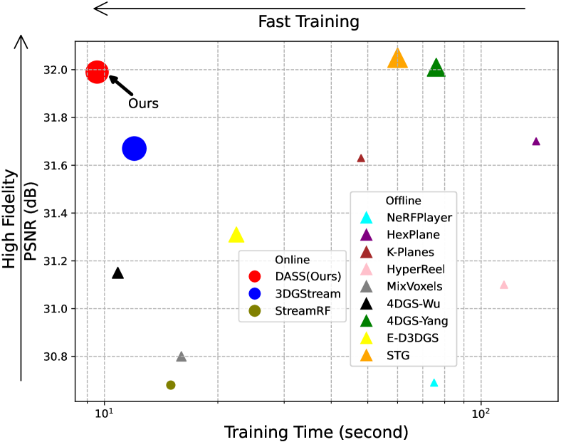
Figure 1: Performance of 4D dynamic spatial reconstruction methods in terms of per-frame training time and reconstruction quality (PSNR) on the N3DV dataset [26]. Online methods are represented by circles, while offline methods are indicated by triangles. The size of each marker is proportional to the rendering speed (FPS). Our method achieves the fastest online training speed, superior reconstruction quality, and real-time rendering performance.

1 Introduction

The rapid advancements of stereoscopic cameras and rendering techniques have expanded human visual perception from 2D planes to spatial 3D representations. This evolution has paved the way for 4D dynamic free-viewpoint video (FVV) reconstruction by integrating the temporal dimension, which unlocks substantial potential for a wide range of applications, including augmented/virtual reality (AR/VR) [1] and holographic communications [41]. Nevertheless, constructing 4D dynamic FVVs from multi-view 2D inputs remains a significant challenge.

In recent years, Neural Radiance Field (NeRF) [33] has emerged as a promising approach for spatial representation and reconstruction. NeRFs optimize neural networks to estimate color and density based on spatial position and viewpoint for 3D reconstruction using captured multi-view inputs. The extensions of NeRFs to dynamic scene reconstruction have demonstrated significant effectiveness [26, 35, 37, 14, 15], yielding photo-realistic novel view synthesis results. However, the efficiency of NeRF-based methods is severely hindered by their low rendering speed due to the dense queries of neural networks. To address this issue, 3D Gaussian Splatting (3DGS) [21] has been proposed as a solution to provide high-quality reconstruction and real-time rendering capabilities, leveraging its flexible point-based primitive design and tile-based differentiable rasterization. Subsequent research efforts [19, 52, 27, 47, 3] have been dedicated to applying Gaussian Splatting for 4D dynamic reconstruction, with representative works integrating the time dimension into each Gaussian primitive [52] or learning spatio-temporal deformations [27, 47].

Despite these advancements, most NeRF-based and 3DGS-based methods for dynamic spatial reconstruction rely on full-length multi-view videos, i.e., non-causal inputs. This reliance overlooks applications such as live streaming, where only per-frame causal inputs are available and on-the-fly training is required. This scenario is formalized as iteratively reconstructing 3D space at the current frame based on previous reconstruction caches and current multi-view inputs. The key challenges in this context are two-fold: (i) how to model temporal variations between frames in 3D space and (2) how to facilitate the optimization convergence from the previous frame to the current one. Critical metrics in this scenario include both the quality of novel view synthesis and streaming time efficiency.

One intuitive solution is to directly optimize a new set of 3DGS primitives for each frame. However, tuning and storing all 3DGS parameters for each frame results in significant time costs and storage overhead. A representative baseline, 3DGStream [38], efficiently optimizes the transformation of Gaussian positions and rotation quaternions, and adaptively densifies a small number of new Gaussians. Although this method achieves fast and high-quality results, it overlooks the difference between inherent dynamics and statics in the scene, instead treating the whole scene uniformly. When modeling movements in the space, dynamic and static components showcase different deformation characteristics. For instance, moving objects, such as humans or animals, may display substantial dynamics, with the Gaussian properties like position experiencing significant offsets. In contrast, static background and stationary objects show minimal movement, where Gaussians remain unchanged or undergo slight jitters. Besides, in most natural scenes, only a small subset of Gaussian primitives corresponds to dynamic areas. Consequently, uniformly modeling the transformation of all Gaussians results in a sub-optimal solution. Moreover, renewing the added Gaussian primitives for each frame fails to fully exploit the temporal continuity.

Based on these insights, we propose a dynamics-aware 3DGS streaming paradigm for on-the-fly 4D reconstruction, termed DASS, where the optimization of each frame comprises three stages: inheritance, shift, and densification. Specifically, considering the temporal continuity, the newly added Gaussians in the previous frame are likely to persist in subsequent frames. Therefore, instead of renewing these added Gaussians for each frame and optimizing them from scratch, we propose a selective inheritance mechanism to adaptively include a portion of the added Gaussians from the previous frame using a learnable selection mask. Then, in the shift stage, we employ 2D dynamics-related prior optical flow [48, 49, 45] and Gaussian segmentation [53, 36] to calculate a per-Gaussian dynamics mask. Subsequently, we assign grid-based layers to learn the offsets of dynamic and static Gaussians with different representation complexities. In the densification stage, apart from the Gaussian offsets that present the deformations of existing objects, new Gaussian primitives are introduced to accommodate newly emerging objects. In this stage, both positional gradients and error maps from the shift stage serve as criteria for identifying regions that require densification. The inheritance stage in the subsequent frame will process these added Gaussians, thereby mitigating errors in the shift stage and reducing the optimization burden in the densification stage. This three-stage pipeline effectively captures dynamic spatial components and exploits the temporal correlation, providing fast on-the-fly training and high-fidelity streaming. Our main contributions are summarized as follows:

• We propose a novel three-stage pipeline for 4D dynamic spatial reconstruction that supports on-the-fly training and per-frame streaming. Our method builds on causal inputs and eliminates the need for full-length multi-view videos, thereby enhancing the practicability.

• Our approach seamlessly integrates the three stages to optimize the reconstruction quality. By selectively inheriting newly introduced Gaussians from the preceding frame, effectively distinguishing dynamic primitives to allocate optimization emphasis, and enhancing areas with weak reconstruction using gradient information and optimization errors, our method ensures high-fidelity dynamic spatial reconstruction.

• Extensive experiments demonstrate the superiority of our method in multiple aspects, including a 20% improvement in online training speed, superior reconstruction quality, and real-time rendering capability.

2 Related Works

2.1 Neural Static Scene Representation

In recent years, reconstructing 3D representations from 2D plane visual inputs has experienced significant advancements, driven by the development of NeRF [33]. NeRF-based methods represent spatial scenes by optimizing multi-layer perceptrons (MLPs) and generate novel views through volume rendering [18]. Subsequent research has enhanced both the training and rendering efficiency through grid-based designs [34, 50, 13, 14]. Nonetheless, NeRF-based approaches typically require dense ray tracing and struggle to fulfill high-speed rendering. Recently, 3DGS [21] has emerged to address these limitations by utilizing explicit unstructured scene representation while preserving point-based differentiable splatting rendering [57]. This approach achieves real-time rendering speed and photo-realistic quality. Based on these advancements, subsequent studies have further enhanced the representation efficiency [31, 8, 30, 11, 24, 55], developed feed-forward reconstruction models [56, 29, 6, 17], and expanded applications in understanding and editing [53, 7, 36, 44].

2.2 Neural Dynamic Scene Reconstruction

Extending static scene representation to dynamic FVV reconstruction remains a significant challenge, primarily due to the difficulties in modeling temporal correlations and variations in 3D space. To address this issue, several studies have extended NeRF to incorporate spatio-temporal structures [25, 5, 37, 14, 42], facilitating dynamic space reconstruction. Similarly, dynamic scene reconstruction methods based on Gaussian Splatting have been proposed, which can be categorized into deformation-based methods, 4D primitive-based methods, and iterative streaming methods. Deformation-based methods [47, 32, 51, 3] maintain 3D Gaussian representations and optimize a neural deformable field to capture temporal variations. 4D primitive-based methods [52, 27, 54] augment Gaussian primitives by integrating the temporal axis as an intrinsic property, thereby directly learning the spatio-temporal distributions. Note that both categories of methods rely on full-length multi-view videos for training, which limits their ability to support on-the-fly training and per-frame streaming. In contrast, iterative streaming methods build upon previously converged representations and perform per-frame optimization for each frame’s multi-view inputs, thereby addressing the above limitations. However, this area remains largely underexplored. Our work aims to develop an iterative streaming pipeline that accelerates per-frame optimization convergence and enhances the reconstruction quality.

The work most closely related to ours is 3DGStream [38]. It proposes a two-stage optimization process for each frame, where the first stage optimizes a grid-based MLP [34] for Gaussian property transformation and the second stage wisely adds new Gaussians based on positional gradients. However, 3DGStream does not consider the intrinsic dynamic and static features in the scene and erases the added primitives in each frame, which neglects the temporal consistency. We have also noticed several concurrent studies on iterative 4D reconstruction, although their focuses differ from ours. For instance, S4D [16] directly manipulates 3D control points to guide the movements, but it requires full optimization that incurs significant time costs on key frames. V³ [43] aims to facilitate streaming free-viewpoint videos on mobile devices, with a particular emphasis on the reduction of the per-frame streaming storage overhead. Conversely, our work identifies the per-frame convergence speed as the critical bottleneck. Moreover, while V³ decomposes motion and appearance attributes for efficient reconstruction, it primarily applies to scenarios with moving objects against vacant background and does not accommodate emerging objects. In addition, SwinGS [28] concentrates on maintaining a consistently stable stream data volume over time and reducing storage overhead through the use of Markov Chain Monte Carlo [22] and a window-based design. Another work [39] considers the bit allocation in a system-level implementation. In contrast, our work focuses on achieving fast convergence in per-frame optimization while maintaining high reconstruction quality, which is orthogonal to the contributions of aforementioned studies.

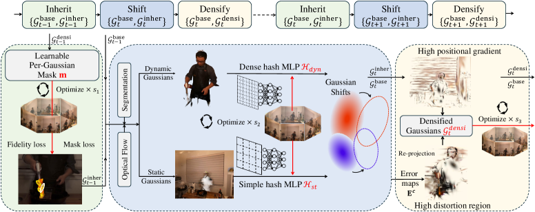
Figure 2: Overview of our proposed DASS framework. The selective inheritance stage (Green) exploits the temporal continuity and adaptively preserves Gaussians from the previous frame. The dynamics-aware shift stage (Blue) distinguishes the dynamic and static elements and optimizes the deformations. The error-guided densification stage (Yellow) detects and densifies the areas with weak reconstruction based on positional gradients and distortions. Variables highlighted in red represent learnable parameters in each stage, whose training is significantly lightweight compared to tuning all Gaussian parameters.

3 Methodology

3.1 Overview

Our method, referred to as DASS, achieves 4D dynamic spatial reconstruction in an iterative manner, enabling on-the-fly training and per-frame streaming. At each timestep $t$, the optimization begins with the representation of the previous timestep, denoted by $\bm{\mathcal{G}}_{t-1}$, to derive the current representation $\bm{\mathcal{G}}_{t}$, based on the current multi-view inputs from $C$ viewpoints. For each scene, the pipeline starts from an initial set of 3D Gaussians at frame 0. This initial representation $\bm{\mathcal{G}}_{0}$ consistently serves as a base representation $\bm{\mathcal{G}}^{\textrm{base}}$ with a constant number of primitives $N$ across subsequent frames. Moreover, each timestep incorporates a varying yet limited number of densified Gaussians, denoted by $\bm{\mathcal{G}}^{\textrm{densi}}$, to model the unique per-frame objects. A subset of these densified Gaussians is inherited to the next timestep as $\bm{\mathcal{G}}^{\textrm{inher}}$.

Fig. 2 depicts an overview of our DASS framework, where the optimization for each frame comprises three stages: inheritance, shift, and densification. Unlike previous methods that regenerate densified Gaussians at each timestep without considering temporal continuity, our approach introduces a selective inheritance stage (Sec. 3.2) at the beginning of optimization for each timestep. During this stage, the densified Gaussians from the preceding timestep, $\bm{\mathcal{G}}^{\textrm{densi}}_{t-1}$, are selectively inherited using a per-Gaussian learnable mask. This mask effectively eliminates redundant Gaussians while preserving essential ones, transforming the set from $\{\bm{\mathcal{G}}^{\textrm{base}}_{t-1},\bm{\mathcal{G}}^{\textrm{densi}}_{t-1}\}$ to $\{\bm{\mathcal{G}}^{\textrm{base}}_{t-1},\bm{\mathcal{G}}^{\textrm{inher}}_{t-1}\}$. Then, the shift stage (Sec. 3.3) processes the base Gaussians $\bm{\mathcal{G}}^{\textrm{base}}_{t-1}$ and the inherited densified Gaussians $\bm{\mathcal{G}}^{\textrm{inher}}_{t-1}$. In this stage, a Gaussian-level dynamics mask is estimated to categorize the Gaussians into dynamic and static groups. These categories are then processed by two hash-encoding MLPs that operate at different complexities. This shift stage efficiently manages the movements and rotations of Gaussian primitives, accommodating changes from the previous timestep and updating the representation as $\{\bm{\mathcal{G}}^{\textrm{base}}_{t-1},\bm{\mathcal{G}}^{\textrm{inher}}_{t-1}\}\to\{\bm{\mathcal{G}}^{\textrm{base}}_{t},\bm{\mathcal{G}}^{\textrm{inher}}_{t}\}$. In the densification stage (Sec. 3.4), emerging objects, such as coffee being poured from a cup and flames from an oven, are identified by analyzing positional gradients and distortions resulted from the shift stage. Then, this stage densifies additional Gaussian primitives to accurately represent these emerging objects and yields $\{\bm{\mathcal{G}}^{\textrm{base}}_{t},\bm{\mathcal{G}}^{\textrm{inher}}_{t}\}\to\{\bm{\mathcal{G}}^{\textrm{base}}_{t},\bm{\mathcal{G}}^{\textrm{densi}}_{t}\}$. Our proposed design facilitates fast per-frame convergence and produces high-fidelity view synthesis results. The details of each stage are elaborated in the following subsections.

3.2 Selective Inheritance

In our pipeline, the shift and densification stages focus on the deformation of existing objects and the densification for emerging objects, respectively. Due to the strong temporal consistency inherent in the scene, the densified Gaussians from the previous frame, $\bm{\mathcal{G}}^{\textrm{densi}}_{t-1}$, are likely to persist and remain valid in the current frame, since they have been specifically optimized for the scene. Leveraging these frame-wise priors and dependencies for subsequent frames can significantly accelerate on-the-fly training convergence. However, previous methods, such as 3DGStream [38], typically avoid reusing these Gaussians to prevent the accumulation of an excessive number of Gaussians, which can lead to prohibitive training and streaming overhead. To address this limitation, we propose a selective inheritance mechanism for the densified Gaussian primitives $\bm{\mathcal{G}}^{\textrm{densi}}_{t-1}$. This approach adaptively selects a subset of the Gaussians that are beneficial for the reconstruction while controlling the total number of Gaussians to avoid excessive accumulation.

Specifically, for each Gaussian primitive in $\bm{\mathcal{G}}^{\textrm{densi}}_{t-1}$, we assign a learnable parameter. The parameter vector for these Gaussians is denoted by $\mathbf{m}$. We then apply the sigmoid function to $\mathbf{m}$, yielding $\textrm{sigmoid}(\mathbf{m})$, followed by quantization to generate a binary mask. This mask indicates the existence of inherited Gaussians, which is element-wise multiplied with the Gaussian opacities and scales as follows:

$$\mathbf{o}_{r} =\textrm{Quant}(\textrm{sigmoid}(\mathbf{m}))\circ\mathbf{o},$$ (1)

$$\mathbf{s}_{r} =\textrm{Quant}(\textrm{sigmoid}(\mathbf{m}))\circ\mathbf{s},$$

where $\mathbf{o}_{r}$ and $\mathbf{s}_{r}$ are the opacity and scale values used during rendering, $\mathbf{o}$ and $\mathbf{s}$ are the original opacity and scale values, and $\circ$ represents the element-wise multiplication. When the mask is quantized to zero, the corresponding Gaussian has zero opacity and scale, thus contributing nothing to the rendering process. Therefore, this mask determines whether each Gaussian is retained in the rendering. By optimizing $\mathbf{m}$, the method selectively inherits the most relevant densified Gaussians from $\bm{\mathcal{G}}^{\textrm{densi}}_{t-1}$. The loss function for optimizing $\mathbf{m}$ is expressed as follows:

$$\mathcal{L}=(1-\lambda)\mathcal{L}_{1}+\lambda\mathcal{L}_{\textrm{D-SSIM}}+\lambda_{\textrm{inher}}\sum\textrm{sigmoid}(\mathbf{m}).$$ (2)

The first two terms represent the fidelity loss in the vanilla 3DGS [21], where $\mathcal{L}_{1}$ and $\mathcal{L}_{\textrm{D-SSIM}}$ are pixel-level $L_{1}$ loss and D-SSIM [46] loss, respectively. The final term, weighted by $\lambda_{\textrm{inher}}$, is referred to as the mask loss and serves as a regularizer that encourages the parameters in $\mathbf{m}$ to approach zero. This regularization effectively reduces the number of inherited Gaussians and controls the numerical accumulation, while the fidelity loss aims to keep the Gaussians that are beneficial for reconstruction. Consequently, this trade-off optimizes the learnable $\mathbf{m}$ and selectively inherits important Gaussians from $\bm{\mathcal{G}}^{\textrm{densi}}_{t-1}$. After $s_{1}$ optimization steps, the final optimized mask $\textrm{Quant}(\textrm{sigmoid}(\mathbf{m}))$ is employed to remove redundant densified Gaussians and preserve the important ones as $\bm{\mathcal{G}}^{\textrm{inher}}_{t-1}$, which is subsequently fed into the following shift and densification stages.

This selective inheritance enhances the optimization pipeline in two key aspects. First, when training at timestep $t$ with the previous timestep’s base Gaussians $\bm{\mathcal{G}}^{\textrm{base}}_{t-1}$, distortions may occur due to temporal transformations and emerging objects. Feeding the base Gaussians directly into the shift stage can lead to inaccurate adjustments in Gaussian properties. Selectively inheriting the previous densified Gaussians $\bm{\mathcal{G}}^{\textrm{inher}}_{t-1}$ before the shift stage mitigates these optimization errors. Second, after the selective inheritance and shift stages, we obtain a refined set of optimized Gaussians $\bm{\mathcal{G}}^{\textrm{inher}}_{t}$, which reduces the number of densified Gaussians requiring optimization, thus improving training efficiency.

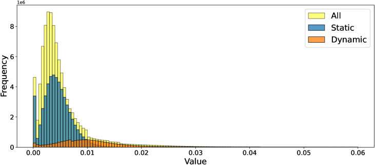
Figure 3: Histogram of Gaussian deformations in the flame steak scene of the N3DV dataset [26]. The overall distribution of Gaussian deformations (Yellow) is widely spread, with the majority falling into the low deformation range (less than 0.01). The dynamic (Orange) and static (Blue) components display different deformation patterns, where significant transformations are mainly concentrated in the dynamic component and minimal transformations are primarily found in the static component.

3.3 Dynamics-Aware Shift

In this stage, we focus on modeling the movements and rotations of Gaussian primitives from the preceding frame to the current one. A common approach to achieve this is directly learning deformation fields to accommodate temporal transformations, as in previous deformation-based method [47] and iterative streaming method [38]. However, these approaches often overlook the significant diversity in the movements of Gaussian primitives present in natural scenes, which can result in slower convergence. Specifically, Gaussians representing background or stationary object typically show high similarity with minimal variations or remain unchanged, while those in the foreground, such as humans, animals, and other moving objects, display significant dynamics. This disparity is illustrated in Fig. 3, which presents a histogram of Gaussian positional offsets between frames in the flame steak scene of N3DV [26]. We observe that most offsets fall within the range of $(0,0.01]$, which indicates that the majority of Gaussians undergo only minor shifts. Therefore, it is inappropriate to optimize the diverse variations in the scene using a single deformation field.

To address this, we propose estimating a per-Gaussian dynamics mask for $\bm{\mathcal{G}}_{t-1}=\{\bm{\mathcal{G}}^{\textrm{base}}_{t-1},\bm{\mathcal{G}}^{\textrm{inher}}_{t-1}\}$ before deformation. This mask is used to categorize all primitives into dynamic and static groups. Then, we assign two deformation layers to learn the respective Gaussian transformations: A complex hash-encoding MLP [34] to capture the intricate shifts and rotations in the dynamic group, and a simpler hash-encoding MLP to model the regionally similar minor variations in the static group.

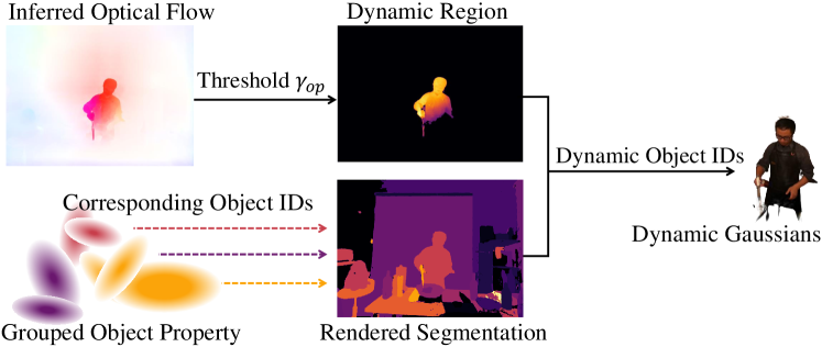
Figure 4: Pipeline of obtaining the per-Gaussian dynamics mask. The process begins with optical flow and segmentation, which provide 2D priors to identify the dynamic object IDs. These IDs are then used to find the corresponding Gaussians in the 3D space.

To construct the per-Gaussian dynamics mask, we leverage established techniques from optical flow [48, 49, 45] and segmentation [23, 20, 53, 36]. Specifically, we utilize Gaussian Grouping [53] to initialize the scene $\bm{\mathcal{G}}_{0}$, which assigns an object property, akin to color property, to each Gaussian primitive and optimizes this property with 2D segmentation results serving as ground truth. These object properties provide per-Gaussian segmentation results that connect 2D images with 3D Gaussians, which facilitates the rendering of segmentation results on any viewpoint. Notably, these object properties remain fixed in subsequent frames $\bm{\mathcal{G}}_{t}(t>0)$, thus posing no additional burden on the time efficiency of on-the-fly training. For subsequent frames, we infer an optical flow estimation network [49] from consecutive frames captured from the same viewpoint and identify the areas where the optical flow exceeds a threshold $\gamma_{op}$, which we classify as dynamic areas. We then query the rendered segmentation results to find out the dynamic object IDs. The dynamic Gaussians are consistently detected using these IDs, as shown in Fig. 4. This process utilizes off-the-shelf methods that do not require network training, allowing us to obtain the per-Gaussian dynamics mask within milliseconds (about 300 ms). An introduction of these methods is provided in the supplementary material.

After obtaining the dynamics mask, we employ the multi-resolution hash-encoding layer I-NGP [34] to learn the deformations. For each Gaussian, the deformation includes a position offset $\bm{\mu}_{n}\in\mathbb{R}^{3}$, which is added to the Gaussian position $\bm{p}_{n}$, and a rotation offset $\bm{\sigma}_{n}\in\mathbb{R}^{4}$, which is applied to the Gaussian rotation quaternion $\bm{q}_{n}$ by using $\mathrm{norm}({\bm{q}_{n}})\times\mathrm{norm}(\bm{\sigma}_{n})$. Here, $\mathrm{norm}(\cdot)$ denotes the normalization operation. The expressive ability of I-NGP is affected by the network complexity parameters, including the hash table size $T_{\textrm{Hash}}$ and the number of feature dimensions per entry $F_{\textrm{Hash}}$. For the dynamic group, we utilize a large-sized hash-encoding layer $\mathcal{H}_{\textrm{dyn}}$ with $T_{\textrm{Hash}}=T_{\textrm{large}}$ and $F_{\textrm{Hash}}=F_{\textrm{large}}$ to accommodate the complex variations of dynamic Gaussians. In contrast, for the static group, we employ a simpler hash-encoding layer $\mathcal{H}_{\textrm{st}}$ with $T_{\textrm{Hash}}=T_{\textrm{large}}/4$ and $F_{\textrm{Hash}}=F_{\textrm{large}}/2$, conserving computational resources while effectively managing minor jitters in background and stationary objects. These lightweight networks are optimized and provide a more efficient alternative to directly tuning the parameters of all Gaussians. To train $\mathcal{H}_{\textrm{dyn}}$ and $\mathcal{H}_{\textrm{st}}$, we use the fidelity loss function as follows:

$$\mathcal{L}=(1-\lambda)\mathcal{L}_{1}+\lambda\mathcal{L}_{\textrm{D-SSIM}}.$$ (3)

Fig. 3 also depicts the optimized deformation distributions of $\mathcal{H}_{\textrm{dyn}}$ and $\mathcal{H}_{\textrm{st}}$ in the flame steak scene. The different deformation patterns observed in the dynamic and static groups validate the effectiveness of our proposed strategy.

3.4 Error-Guided Densification

The above two stages inherit temporally continuous Gaussians and manage deformations, without introducing new Gaussians. However, similar to the vanilla 3DGS [21] and 4DGS [52], densification remains essential to address areas with insufficient reconstruction quality and new objects.

To achieve fast and high-quality densification, it is crucial to identify the subset of Gaussians in need of densification. Previous methods [21, 38] detect these under-reconstructed Gaussians based on historical view-space positional gradients, denoted by $\overline{\nabla\mathbf{p}}\triangleq\{\overline{\nabla p_{n}},\forall n\}\in\mathbb{R}^{N\times 1}$. This approach tracks gradients from previous training steps and densifies Gaussians whose positional gradients exceed a specific threshold $\tau_{\textrm{pos}}$. While this criterion effectively identifies general regions with inadequate reconstruction, it does not provide sufficient emphasis on regions with emerging objects or significant reconstruction errors. This limitation can hinder the efficient optimization of emerging objects, potentially slowing the convergence of on-the-fly training. To address this, we propose an error-adaptive densification strategy that incorporates an additional indicator to identify Gaussians that require densification. This approach projects high-distortion areas from the image space to the 3D space and adaptively enhances densification in critical areas.

Specifically, we collect 2D error maps by comparing the ground truth with the rendered results in the shift stage for each training viewpoint, denoted by $\mathbf{E}^{c}$, $c=1,2,\cdots,C$. Then, we filter out the pixel positions with severe distortion above $\gamma_{\textrm{err}}$, yielding an $H\times W$ binary matrix $\mathbf{D}_{\textrm{err}}^{c}=\{\mathbf{1}[e_{i}^{c}>\gamma_{\textrm{err}}],\forall e^{c}_{i}\in\mathbf{E}^{c},i=1,\cdots,H\times W\}$ in the 2D pixel plane, where $\mathbf{1}[\cdot]$ is the binary indicator function. Next, we project the positions of the 3D Gaussians $\bm{\mathcal{G}}^{\textrm{base}}$ onto the 2D image plane as $(\mathbf{X},\mathbf{Y})=\text{Proj}(\bm{\mathcal{G}}^{\textrm{base}})$, where $\mathbf{X}\triangleq\{\mathbf{x}_{n},\forall n\},\mathbf{Y}\triangleq\{\mathbf{y}_{n},\forall n\}$, with $(\mathbf{x}_{n},\mathbf{y}_{n})$ representing the 2D pixel coordinate of the $n$-th Gaussian primitive along the $H$ and $W$ axes. The projection $\text{Proj}(\cdot)$ utilizes the known intrinsic and extrinsic camera matrices, with further details provided in the supplementary material. We then identify the subset of Gaussians that fall within the erroneous areas for each viewpoint, represented as $\mathcal{S}^{c}_{\textrm{err}}=\{\bm{\mathcal{G}}^{\textrm{base}}|\mathbf{D}_{\textrm{err}}^{c}(\mathbf{x}_{n},\mathbf{y}_{n})=1,\forall n\}$.

For these highlighted Gaussian primitives, we apply a relatively lower gradient threshold $\tau_{\textrm{err}}<\tau_{\textrm{pos}}$, thereby placing greater emphasis on high-distortion areas and facilitating more effective error rectification compared to strategies that rely only on a single indicator. This leads to an error-guided adaptive densification scheme, yielding the subset of Gaussians for densification $\mathcal{S}$ as follows:

$$\mathcal{S}=\{\bm{\mathcal{G}}^{\textrm{base}}|\overline{\nabla p_{n}}>\tau_{\textrm{pos}},\forall n\}\cup\big{\{}\mathcal{S}_{\textrm{err}}\cap\{\bm{\mathcal{G}}^{\textrm{base}}|\overline{\nabla p_{n}}>\tau_{\textrm{err}},\forall n\}\big{\}},$$ (4)

where $\mathcal{S}_{\textrm{err}}=\{\cup^{C}_{c=1}\mathcal{S}^{c}_{\textrm{err}}\}$ is the combination of high-distortion subsets over all viewpoints. This error-guided adaptive subset $\mathcal{S}$ prioritizes the defects in historical optimization steps while accommodating under-reconstructed areas. We then perform spawn densification to compensate for both weakly reconstructed regions and emerging objects, following the vanilla 3DGS [21] and 3DGStream [38]. The newly added Gaussians, along with the transformed inherited Gaussians $\bm{\mathcal{G}}^{\textrm{inher}}_{t}$, are optimized using the fideltiy loss function as in Eq. (3) to yield $\bm{\mathcal{G}}^{\textrm{densi}}_{t}$. During this optimization, the pruning strategy is employed to eliminate excessive Gaussian candidates with very low opacity. Notably, these densified Gaussians $\bm{\mathcal{G}}^{\textrm{densi}}_{t}$ constitute only a small fraction of the total number of primitives in the scene, significantly saving computational and time costs compared to full-scene optimization.

3.5 Summary

Our proposed pipeline, DASS, effectively achieves iterative streamable 4D reconstruction through the seamless integration of the above three stages. The inheritance stage selectively preserves the optimized densified Gaussians from the previous frame. By exploiting the temporal consistency, this stage compensates for distortions caused by emerging objects before the shift stage and alleviates the optimization burden in the subsequent densification stage. The dynamics-aware shift stage incorporates separate deformation fields for dynamic and static features. This design is tailored to accommodate complex movements in the dynamic elements while conversing optimization resources for static components. After solving the temporal deformations, the error-guided densification stage reconstructs emerging objects in the current frame. It employs both positional gradients and rendering distortions as references to effectively identify the areas with weak reconstruction and emerging elements. Collectively, these three stages enable DASS to achieve high-fidelity reconstruction while significantly accelerating on-the-fly optimization.

4 Experiments

4.1 Experimental Setup

Datasets. To evaluate the effectiveness of our pipeline, we employ two real-world benchmark datasets that are representative of 4D scene reconstruction and streaming tasks. (1) Neural 3D Video (N3DV) dataset [26] comprises six multi-view videos captured from 18 to 21 viewpoints, each at a resolution of $2704\times 2028$. Following previous methods [26, 25, 38, 52, 54], our experiments are conducted at a half resolution of $1352\times 1014$, using one view for evaluation and the remaining views for training. (2) Meet Room dataset, provided by the previous work on the streaming task [25], includes videos at a resolution of $1280\times 720$ and a frame rate of 30 FPS. This dataset is captured from 13 viewpoint cameras, which is relatively sparser than N3DV. Consistent with the baselines [25, 38], one view is reserved for testing and the other twelve views are used for training.

Implementation. We initiate our training at timestep 0 using Gaussian Grouping [53] and optimize the object properties for segmentation concurrently during this initialization, after which these properties remain fixed for subsequent frames. The optical flow is directly inferred using Unimatch [49]. These off-the-shelf methods obtain the segmentation and optical flow results without requiring extra pre-training, thereby imposing minimal computational or temporal overhead during on-the-fly training and streaming. For subsequent timesteps, the optimization processes for the inheritance, shift, and densification stages are executed with $s_{1}=20$, $s_{2}=100$, and $s_{3}=60$ steps, respectively.

Table 1: Quantitative comparison on the N3DV dataset. The training time and reconstruction qualities are averaged over all 300 frames for each scene. ^†DyNeRF only reports metrics for the flame salmon scene. ^‡STG trains each model using a 50-frame video sequence, requiring six models to complete the representation.

Category	Method	PSNR$\uparrow$	DSSIM$\downarrow$	Train	Render$\uparrow$	Streamable
		(dB)		Time$\downarrow$	(FPS)
Static	Plenoxels [13]	30.77	-	$>$1000 s	8.3	$\checkmark$
	I-NGP [34]	28.62	-	79 s	2.9	$\checkmark$
Offline	DyNeRF† [26]	29.58	-	$>$1000 s	0.02	$\times$
	NeRFPlayer [37]	30.69	0.0340	75 s	0.05	$\checkmark$
	HexPlane [5]	31.70	-	140 s	0.21	$\times$
	K-Planes [14]	31.63	-	48 s	0.15	$\times$
	HyperReel [2]	31.10	0.0360	115 s	2	$\times$
	MixVoxels [42]	30.80	-	16 s	16.7	$\times$
	4DGS-Wu [47]	31.15	0.0331	10.85 s	30	$\times$
	4DGS-Yang [52]	32.01	0.0290	76 s	114	$\times$
	E-D3DGS [3]	31.31	0.0259	22.4 s	74.5	$\times$
	STG‡ [27]	32.05	0.0261	60 s	140	$\times$
Online	StreamRF [25]	30.68	-	15 s	8.3	$\checkmark$
	3DGStream [38]	31.67	-	12 s	215	$\checkmark$
	DASS (Ours)	31.99	0.0285	9.62 s	189.2	$\checkmark$

Baselines. Our primary comparisons are against iterative 4D dynamic spatial reconstruction methods that support on-the-fly training and per-timestep streaming, specifically StreamRF [25] and 3DGStream [38], which are categorized as online methods. To evaluate reconstruction fidelity, we also include other 4D dynamic spatial reconstruction methods that require full-length multi-view videos as input and do not support on-the-fly training or per-timestep streaming. This offline category includes NeRF-based methods such as DyNeRF [26], NeRFPlayer [37], HexPlane [5], K-Planes [14], HyperReel [2], and MixVoxels [42], as well as recent 3DGS-based methods like 4DGS-Wu [47], 4DGS-Yang [52], E-D3DGS [3], and STG [27]. Note that NeRFPlayer [37] allows streaming after optimization but does not support on-the-fly training. In addition, we consider static methods, including Plenoxels [12] and I-NGP [34], which fully train a static scene representation for each frame.

Metrics. We focus on achieving fast on-the-fly training for streamable dynamic spatial reconstruction, emphasizing both time efficiency and reconstruction fidelity. To evaluate time efficiency, we calculate the average per-frame training time over the 300 frames in the video and measure the frames per second (FPS). For offline methods that do not support on-the-fly training, we report their training time averaged over all frames. To assess reconstruction fidelity, we use metrics including peak signal-to-noise ratio (PSNR) and dissimilarity structural similarity index measure (DSSIM).

Table 2: Quantitative comparison on the Meet Room dataset. The training time and quality metrics are averaged over all 300 frames.

Method	PSNR (dB)$\uparrow$	Train Time (s)$\downarrow$	Render (FPS)$\uparrow$
Plenoxels [13]	27.15	840	10
I-NGP [34]	28.10	65	4.1
StreamRF [25]	26.72	10.2	10
3DGStream [38]	30.79	6	288
DASS (Ours)	30.81	5.04	253.8

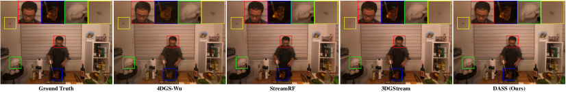
Figure 5: Qualitative comparison for the flame steak scene of the N3DV dataset, including online training methods [25, 38] and offline reconstruction method [47]. Compared to other methods, our method accurately recovers dynamic objects and preserves intricate details.

4.2 Results and Comparisons

The quantitative evaluation results of our method on the N3DV dataset [26] are detailed in Tab. 1, and a comprehensive comparison of multiple metrics is shown in Fig. 1. Our method achieves the fastest on-the-fly training speed, which converges from previous frame to the current one within 10 seconds, yielding a 20% improvement in efficiency. In contrast, the average training time of baseline methods ranges from tens of seconds to several minutes. This time efficiency advantage originates from several aspects: First, our inheritance stage effectively captures the temporal continuity and selectively preserves the optimized results from the previous frame. This significantly alleviates the optimization burden in the following stages, especially for the densification stage, which requires 60 steps compared to the 100 steps in 3DGStream. Moreover, the selective inheritance stage is lightweight, as it optimizes only one learnable parameter for each Gaussian primitive, in contrast to the tens of parameters in a pipeline fully dependent on densification. In addition, our dynamics-aware shift stage assigns different deformation layers for dynamic and static components, which focus on significant and subtle variations, respectively. This strategy enhances the convergence achieving high-quality deformations with fewer optimization steps (100 steps instead of 150 steps in 3DGStream). Although our pipeline requires optical flow and segmentation, these results are either directly inferred or rendered within milliseconds and are executed only once every few frames.

Beyond the significant time advantage, the reconstruction fidelity of our method also outperforms previous online streamable baselines [25, 38] and surpasses most state-of-the-art offline training methods [26, 37, 5, 14, 2, 42, 47, 3]. Our dynamics-aware deformation places greater emphasis on areas with complex motions and variations, thereby facilitating more detailed reconstruction. Besides, our error-guided densification strategy identifies areas with weak construction and newly emerging objects, which rapidly detects and mitigates the reconstruction defects. A qualitative comparison on the N3DV dataset is provided in Fig. 5. A detailed comparison of each scene in the N3DV dataset is provided in the supplementary material.

Table 3: Results of ablation experiments, which are averaged over six scenes from the N3DV dataset.

Method	PSNR(dB)$\uparrow$
w/o Inheritance	31.71
w/o Dynamics awareness	31.69
w/o Densification	31.50
w/o Error guidance	31.88
Full Model (Our DASS)	31.99

Our rendering speed further highlights the superiority of our method over others. Leveraging the real-time rasterization, our rendering speed significantly outperforms that of NeRF-based methods. Moreover, our method achieves higher FPS than 4DGS methods, since our deformation fields, comprising only hash encoding and simple MLPs, enable a low query overhead of around 1 ms.

Similarly, our method demonstrates fast on-the-fly training, efficient rendering speed, and high-fidelity reconstruction on the MeetRoom dataset, as detailed in Tab. 2.

4.3 Ablation Studies

We conduct ablation experiments on the N3DV dataset to evaluate the contributions of our proposed designs. Our pipeline comprises three key stages: selective inheritance, dynamics-aware shift, and error-guided densification. To assess the impact of each stage, we either replace it with a baseline counterpart or remove it from the pipeline, and provide reconstruction quality comparisons with fixed optimization steps. The results are summarized in Tab. 3.

Effectiveness of Selective Inheritance. To evaluate the impact of the selective inheritance stage, we remove it from the pipeline, leading to the baseline “w/o Inheritance” in Tab. 3. In this baseline, base Gaussians are directly transformed, and newly added Gaussian are regenerated for each frame. This approach results in a performance degradation of 0.28 dB compared to the full model, since it fails to leverage the temporal continuity and imposes optimization burdens on the following two stages. In contrast, our selective inheritance stage effectively balances the preservation of essential Gaussians while controlling numerical accumulation. We also visualize the error maps before and after the inheritance stage in Fig. 6, which demonstrates that our selective inheritance strategy effectively enhances temporal coherence and reduces the optimization overhead for subsequent stages.

Effectiveness of Dynamics-Aware Shift. To validate the improvement of our dynamics-aware shift strategy, we replace the dynamics-aware deformation fields with one universal hash-encoding MLP, referred to as “w/o Dynamics awareness” in Tab. 3. This baseline shows a performance drop of 0.3 dB, which underscores the importance of our dynamics-aware optimization in highlighting the intrinsic dynamics and statics in the space and effectively managing the complex movements.

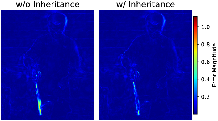
Figure 6: Error map visualization without (left) and with (right) the proposed selective inheritance mechanism. The selective inheritance stage effectively compensates for the artifacts in temporally consistent area and mitigates the optimization distortions.

Effectiveness of Error Guided Densification. To evaluate the effectiveness of our error-guided densification, we consider two baselines for comparison. The first “w/o Densification” baseline excludes the densification stage and results in a significant decline in quality. This suggests that solely relying on transformations of existing Gaussian primitives is inadequate for representing dynamic scenes. The second baseline, “w/o Error guidance”, removes the error-guided subset $\mathcal{S}_{\textrm{err}}$ from the densification process and uses only the gradient indicator, leading to degraded performance. This indicates that our error-guided densification effectively caters for under-reconstructed areas and emerging objects.

5 Conclusion

In this paper, we introduce a novel three-stage pipeline for iterative online 4D dynamic spatial reconstruction, which allows for on-the-fly training and per-frame streaming. We incorporate a selective inheritance stage to capture the temporal continuity, a dynamics-aware shift stage to exploit the dynamic and static features in natural scenes, and an error-guided densification stage to adaptively recover emerging objects and weak reconstruction. Our method achieves state-of-the-art performance in online streaming 4D reconstruction, providing the fastest training speed, with a 20% improvement, and superior representation quality.

Appendix

The supplementary material provides an introduction of preliminary knowledge in Sec. A, more implementation details in Sec. B, additional experimental results in Sec. C, and discusses potential extensions in Sec. D.

Appendix A Preliminaries

A.1 3D Gaussian Splatting

3D Gaussian Splatting (3DGS) [21] exploits a point-based representation to reconstruct 3D space from multi-view image inputs. A Gaussian primitive is expressed as:

$$G(\bm{x})=e^{-\frac{1}{2}(\bm{x}-\bm{\mu})^{T}\bm{\Sigma}^{-1}(\bm{x}-\bm{\mu})},$$ (5)

where $\bm{\mu}\in\mathbb{R}^{3}$ and $\bm{\Sigma}\in\mathbb{R}^{3\times 3}$ denote the position vector and the covariance matrix, respectively. The covariance matrix $\bm{\Sigma}$ is decomposed into a rotation matrix $\mathbf{R}\in\mathbb{R}^{3\times 3}$ and a scaling matrix $\mathbf{S}\in\mathbb{R}^{3\times 3}$ as:

$$\bm{\Sigma}=\mathbf{R}\mathbf{S}\mathbf{S}^{T}\mathbf{R}^{T},$$ (6)

where $\mathbf{R}$ and $\mathbf{S}$ are further represented by a quaternion $\mathbf{q}\in\mathbb{R}^{4}$ and a vector $\mathbf{s}\in\mathbb{R}^{3}$, respectively. When rendering an image on a 2D plane, this covariance matrix from the 3D space is projected onto the 2D plane as follows:

$$\bm{\Sigma}_{\textrm{2D}}=\mathbf{J}\mathbf{W}\bm{\Sigma}\mathbf{W}^{T}\mathbf{J}^{T},$$ (7)

where $\mathbf{W}$ is the viewing projection matrix and $\mathbf{J}$ is the Jacobian of the affine approximation for the projective transformation. After reconstructing a 3D space with $N$ Gaussian primitives, the rendered RGB image, denoted by $\bm{C}$, is obtained by blending the contributing Gaussians in depth order as follows:

$$\bm{C}=\sum_{i=1}^{N}\bm{c}_{i}\alpha_{i}\prod_{j=1}^{i-1}(1-\alpha_{j}),$$ (8)

where $\alpha_{i}$ denotes the product of the 2D Gaussian with the $i$-th greatest depth and its opacity property $o_{i}$, and $\bm{c}_{i}$ represents its view-dependent color property.

A.2 Gaussian Grouping

As elaborated in the previous subsection, the vanilla 3DGS method assigns position, scale, rotation, opacity, and color attributes to each Gaussian primitive. In addition to these attributes, Gaussian Grouping [53] introduces an additional set of learnable properties $\bm{e}_{i}\in\mathbb{R}^{16}$ to each Gaussian for segmentation, which is referred to as Identity Encoding or object property. Similar to the color property, this object property facilitates rendering on the 2D image plane as follows:

$$\mathbf{M}=\sum_{i=1}^{N}\bm{e}_{i}\alpha_{i}\prod_{j=1}^{i-1}(1-\alpha_{j}),$$ (9)

where $\mathbf{M}$ represents the rendered 2D mask identity feature, which is of the same size as the rendered RGB image. To optimize the object property $\bm{e}_{i}$, Gaussian Grouping first utilizes 2D segmentation method [23] to generate segmentation masks for each multi-view image, and then employs a well-trained zero-shot tracker [9] to maintain consistent segmentation masks across frames. These 2D segmentation masks supervise the optimization of the object property $\bm{e}_{i}$ and a single convolution layer to recover the object property dimension into segmentation classes. This optimization is performed concurrently with the optimization of other visual properties. In this way, each Gaussian primitive is assigned an object property that groups the Gaussians into segmented objects. In our proposed DASS, this Gaussian Grouping technique serves as a bridge between the 2D and 3D representations, which facilitates the identification of dynamic object IDs in the 2D image and their corresponding dynamic 3D Gaussian primitives.

A.3 Optical Flow

Optical flow is a representation of the apparent relative motion between consecutive video frames and used to describe the dynamics and variations on the 2D image plane. Among the abundant advanced methods, we employ the Transformer-based optical flow estimation method [49]. This approach balances accuracy and efficiency without the need of iterative refinements, making it suitable for our on-the-fly training setup.

Specifically, the optical flow estimation can be modeled as finding 2D pixel-wise correspondences between consecutive images on a 2D plane. The images are downsampled and enhanced in the feature space, yielding $\mathbf{F}_{1},\mathbf{F}_{2}\in\mathbb{R}^{\frac{H}{8}\times\frac{W}{8}\times D}$. Then, the feature similarity is calculated as follows:

$$\mathbf{S}=\frac{\mathbf{F}_{1}\mathbf{F}_{2}^{T}}{\sqrt{D}}.$$ (10)

Next, a softmax function is applied to $\mathbf{S}$, yielding a normalized matching distribution for each position in $\mathbf{F}_{1}$ corresponding to $\mathbf{F}_{2}$, represented as $\textrm{softmax}(\mathbf{S})$. The correspondence relationship is then derived by multiplying the pixel grid $\mathbf{U}_{\mathrm{2D}}$ with the matching distribution as:

$$\hat{\mathbf{U}}_{\mathrm{2D}}=\textrm{softmax}(\mathbf{S})\cdot\mathbf{U}_{\mathrm{2D}}.$$ (11)

This leads to the optical flow estimation by calculating the discrepancy between the corresponding pixel coordinates as:

$$\mathbf{V}=\hat{\mathbf{U}}_{\mathrm{2D}}-\mathbf{U}_{\mathrm{2D}}.$$ (12)

An additional self-attention layer is used to propagate and remedy unreliable results in this estimation. To get the original image resolution prediction, RAFT’s upsampling [40] method is utilized to compute the full-resolution optical flow.

Appendix B Additional Implementation Details

B.1 Implementation and Metrics

We implement our streaming pipeline based on the official open-source codebase 3DGStream and strictly follow the evaluation principles. Specifically, the reported training time includes the time consumption for training the initialization at frame 0. This frame 0 initialization process takes 10.18 minutes in our pipeline and is counted into the average training time calculation following the official 3DGStream. Notably, the time consumption of subsequent on-the-fly training takes only 7.59 s for each frame. The experiments are mainly conducted on an RTX A6000 GPU and an Intel Xeon Platinum 8370C CPU.

B.2 Additional Details in Each Stage

Initialization. For the initialization at frame 0, we employ the official codebase of Gaussian Grouping. Following 3DGStream, the spherical harmonics degree is set to 1. The segmentation-related hyperparameters in Gaussian Grouping remain unmodified, as we find that varying these hyperparameters leads to minimal impact on the streaming performance. Moreover, during training the initialization, we introduce an opacity regularization term, written as $-\frac{1}{N}\sum^{N}_{i=1}o_{i}\log(o_{i})$, in addition to the fidelity loss. This opacity regularization encourages the opacity of Gaussian primitives to approach either zero or one, thereby pushing Gaussians to the object surface and naturally pruning nearly transparent Gaussians. This regularization has proven effective in previous works [10, 54] to enhance the representation efficiency and quality.

Selective Inheritance. In our proposed selective inheritance stage, the quantized learnable vector after the sigmoid function, $\textrm{Quant}(\textrm{sigmoid}(\mathbf{m}))$, determines whether to maintain the densified Gaussian primitives from the previous frame. Notably, the quantization operation itself is non-differentiable. Therefore, the Straight Through Estimator (STE) [4] is applied in the optimization of $\mathbf{m}$, which is written as:

$$\mathbf{m}_{\textrm{op}}=\textrm{detach}(\textrm{Quant}(\textrm{sigmoid}(\mathbf{m}))-\textrm{sigmoid}(\mathbf{m}))+\textrm{sigmoid}(\mathbf{m}),$$ (13)

where $\mathbf{m}_{\textrm{op}}$ is the parameter involved in differentiable optimization. Moreover, this selective inheritance is paused every 20 frames, i.e., the inherited Gaussians are erased once for every 20 frames. This strategy considers the typical duration of temporally consistent objects and avoids introducing misleading information during optimization.

Dynamics-Aware Shift. The dynamics-aware shift stage distinguishes the dynamic and static groups of Gaussian primitives in the representation and employs different hash-encoding MLPs, $\mathcal{H}_{\textrm{dyn}}$ and $\mathcal{H}_{\textrm{st}}$, as deformation fields for their optimization. The estimation of dynamic objects usually remains consistent across frames, so repeatedly performing this estimation introduces temporal redundancy into the on-the-fly training. In our pipeline, the estimation of dynamic Gaussian group (as shown in Fig. 4 in the main body of the paper) is performed every 10 frames, considering that the dynamic properties remain stable across adjacent frames. As discussed in Sec. 3.3, the hash table size $T_{\textrm{Hash}}$ and the number of feature dimensions per entry $F_{\textrm{Hash}}$ vary between dynamic and static groups. Specifically, for the N3DV dataset, the dynamic group adopts $T_{\textrm{Hash}}=2^{16}$ and $F_{\textrm{Hash}}=4$ for $\mathcal{H}_{\textrm{dyn}}$, while the static group uses $T_{\textrm{Hash}}=2^{14}$ and $F_{\textrm{Hash}}=2$ for $\mathcal{H}_{\textrm{st}}$. For the Meet Room dataset, the dynamic group employs $T_{\textrm{Hash}}=2^{15}$ and $F_{\textrm{Hash}}=4$, while the static group adopts $T_{\textrm{Hash}}=2^{13}$ and $F_{\textrm{Hash}}=2$.

Error-Guided Densification. In the error-guided densification stage, we identify the Gaussians whose positions fall into high-distortion areas for densification to improve reconstruction and recover emerging objects. The projection of Gaussian positions is detailed in Algorithm 1.

Algorithm 1 Projection of 3D Gaussian positions to 2D image plane pixels

0:  Positions of $N$ 3D Gaussians $\mathbf{P}=[\mathbf{X},\mathbf{Y},\mathbf{Z}]\in\mathbb{R}^{N\times 3}$, rendered image size $H$ and $W$, full projection matrix $\mathbf{T}\in\mathbb{R}^{4\times 4}$ embedded in the 3DGS camera model, which is composed of the camera intrinsic matrix and the extrinsic matrix.

1:  Calculate the projection in homography space as $\mathbf{P}_{\textrm{hom}}=[\mathbf{P},\mathbf{1}]\cdot\mathbf{T}=[\mathbf{p}_{x},\mathbf{p}_{y},\mathbf{p}_{z},\mathbf{p}_{\textrm{hom}}]$.

2:  Normalize the coordinates on the image plane as $\mathbf{x}_{\textrm{norm}}=\mathbf{p}_{x}/\mathbf{p}_{\textrm{hom}}$ and $\mathbf{y}_{\textrm{norm}}=\mathbf{p}_{y}/\mathbf{p}_{\textrm{hom}}$

3:  Obtain the corresponding pixel-level coordinates as $\mathbf{x}_{n}=\textrm{Round}(0.5\cdot((\mathbf{x}_{\textrm{norm}}+1)\cdot$W$-1))$ and $\mathbf{y}_{n}=\textrm{Round}(0.5\cdot((\mathbf{x}_{\textrm{norm}}+1)\cdot$H$-1))$

3:  The corresponding pixels of the 3D Gaussian positions as $(\mathbf{X},\mathbf{Y})=[\mathbf{x}_{n},\mathbf{y}_{n}]$.

Appendix C Additional Experimental Results

C.1 Additional Ablation Studies

Impact of Optimization Steps. To assess the impact of the optimization steps at each stage and illustrate the convergence efficiency of our DASS framework, we adjust the optimization steps and evaluate the reconstruction qualities, as shown in Tab. 4. Our DASS assigns $s_{1}=20$, $s_{2}=100$, and $s_{3}=60$ for the inheritance, shift, and densification stages, respectively, serving as the baseline in the first row of Tab. 4. This assignment contributes to the time efficiency of our method compared to the state-of-the-art baseline 3DGStream [38] (9.62 s compared to 12 s), which assigns a total of 250 optimization steps (150 for transformation and 100 for densification). The baselines with increased optimization steps shown in subsequent rows verify that our DASS achieves optimal convergence with the primary optimization setting. Increasing the optimization steps leads to a negligible improvement in representation quality, less than 0.05 dB, while significantly increasing time consumption, thereby validating our convergence efficiency. This efficiency comes from multiple aspects: Our selective inheritance stage preserves the essential Gaussian primitives of the previous frame’s densified Gaussians and mitigates the optimization distortions with only $s_{3}=20$ steps of optimization. The dynamics-aware shift stage learns the diverse distributions of dynamic and static components, respectively, facilitating the deformation convergence. Besides, assigning a low-complexity deformation field to the static components conserves temporal and computational resources for the majority of the Gaussian primitives. The error-guided densification stage effectively detects and compensates for the distortions, enhancing the reconstruction quality while introducing low temporal overhead. In addition, the last two baselines in Tab. 4 demonstrate that reducing the training steps leads to inferior reconstruction quality, necessitating our optimization step assignment.

Table 4: Ablation study on the numbers of optimization steps, with the results averaged over all six scenes of the N3DV dataset [26].

Inheritance	Shift	Densification	PSNR$\uparrow$	Time$\downarrow$
s1	s2	s3	(dB)	(s)
20	100	60	31.99	9.62
50	100	60	31.96	10.29
20	150	60	32.01	11.78
20	100	100	31.99	10.79
20	150	100	32.03	12.53
20	50	60	31.26	7.41
20	100	30	31.50	8.73

Table 5: Comparison with naive 3DGS methods. The training time and reconstruction qualities are averaged over all 300 frames for each scene of the N3DV dataset [26].

Baseline	PSNR (dB)$\uparrow$	Time (s)$\downarrow$
Naive Per-Frame 3DGS	32.07	615
Intuitive Full-Tuned 3DGS	30.83	11.86
DASS (Ours)	31.99	9.62

C.2 Quantitative Results

In addition to the state-of-the-art 4D reconstruction baselines shown in Tab. 1 in the main body of the paper, we provide comparisons with two variants of naive 3DGS methods in Tab. 5 and Fig. 7. Specifically, we compare our method with a naive streamable baseline, which trains an independent set of 3D Gaussian primitives for each frame, referred to as “Naive Per-Frame 3DGS” in Tab. 5. In this baseline, each frame is trained with the same conditions as the initial zero-frame in streaming methods. Although this naive baseline outperforms all off-the-shelf baselines in 4D reconstruction, it fully trains a set of Gaussian primitives from scratch for each scene, leading to a significant training time overhead of approximately 615 seconds per-frame. In contrast, our DASS effectively models the temporal variations in the 3D space and facilitates a fast convergence between frames. DASS demonstrates competitive streaming quality, with only a negligible gap of 0.08 dB compared to this naive baseline, while consuming merely 1.56% of the training time. This significant improvement highlights the efficiency of DASS. We also compare our method with an intuitive full-tuned baseline, which iteratively tunes all parameters of the Gaussian primitives initialized from the previous timestep, termed “Intuitive Full-Tuned 3DGS” in Tab. 5. Specifically, it initializes the on-the-fly training with the same frame 0 initialization as our DASS and tunes all Gaussian properties for a fixed number of iterations, which yields a similar time consumption to ours. As shown in Tab. 5, a significant performance degradation of 1.16 dB is observed in this baseline. This indicates that the intuitive baseline fails to capture temporal variations between frames under such time efficiency, while our DASS effectively manages and converges these variations with lower temporal overhead.

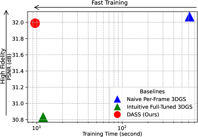
Figure 7: Performance comparisons with two variants of naive 3DGS methods in terms of per-frame training time and reconstruction quality (PSNR) on the N3DV dataset [26]. Our method achieves a much better balance between training efficiency and representation quality.

Besides, we provide the quantitative comparison for each scene of the N3DV dataset [26] detailed in Tab. 6, which is compared with offline training NeRF-based methods [26, 37, 5, 14, 2, 42], offline training 3DGS-based methods [47, 52, 3, 27], online training NeRF-based method [25], and online training 3DGS-based method [38].

Method	Coffee	Cook	Cut	Flame	Flame	Sear	Mean
	Martini	Spinach	Beef	Salmon	Steak	Steak
Plenoxels [13]	27.65	31.73	32.01	28.68	32.24	32.33	30.77
I-NGP [34]	25.19	29.84	30.73	25.51	30.04	30.40	28.62
DyNeRF† [26]	–	–	–	29.58	–	–	29.58
NeRFPlayer [37]	31.53	30.58	29.35	31.65	31.93	29.13	30.69
HexPlane [5]	–	32.04	32.55	29.47	32.08	32.39	31.70
K-Planes [14]	29.99	32.60	31.82	30.44	32.38	32.52	31.63
HyperReel [2]	28.37	32.30	32.92	28.26	32.20	32.57	31.10
MixVoxels [42]	29.36	31.61	31.30	29.92	31.43	31.21	30.80
4DGS-Wu [47]	27.34	32.46	32.90	29.20	32.51	32.49	31.15
4DGS-Yang [52]	28.33	32.93	33.85	29.38	34.03	33.51	32.01
E-D3DGS [3]	29.10	32.96	33.57	29.61	33.57	33.45	31.31
STG‡ [27]	28.61	33.18	33.52	29.48	33.64	33.89	32.05
StreamRF [25]	27.84	31.59	31.81	28.26	32.24	32.36	28.26
3DGStream [38]	27.75	33.31	33.21	28.42	34.30	33.01	31.67
Ours	28.15	33.83	33.54	28.84	34.26	33.33	31.99

Table 6: Quantitative comparison of the PSNR metric across all six scenes of the N3DV dataset, with the value for each scene averaged over 300 frames. ^†DyNeRF only reports results on the flame salmon scene. ^‡STG trains each model with a 50-frame video sequence, requiring six models to complete the overall representation.

C.3 Qualitative Results

We provide additional qualitative results of our method in Fig. 8, Fig. 9, Fig. 10, and Fig. 11. Each figure includes the rendered test view visualizations and comparisons with baseline methods. Our DASS presents high-quality reconstruction and fine visual details compared with the baseline methods. We also provide visualizations of the detected dynamics components, which effectively guides the optimization to focus on dynamic objects and complex motions.

Appendix D Discussion

Our DASS pipeline effectively addresses the challenge of on-the-fly 4D reconstruction for per-frame streaming by integrating selective inheritance, dynamics-aware shift, and error-guided densification stages. These designs have the potential to broaden applications in various 3DGS-based representation tasks. For example, the dynamics-aware strategy effectively detects the dynamic components in the 3D space with available knowledge. This capability particularly enhances applications such as telepresence and holographic communication, where DASS can selectively transmit and stream only the dynamic or human-related components. Consequently, this approach enhances the computational efficiency and reduces communication overhead, which are critical requirements in current 2D online meeting applications. Besides, the error-guided densification proves effective in rapidly compensating for areas with weak reconstruction. It is potential to be extended to further applications where Gaussian densification is performed.

In the aspect of performance improvement, similar to other iterative streamable 4D reconstruction methods, our DASS consistently benefits from the prospective higher quality of initialization, faster rasterization, and improved training strategies in the 3DGS field, as well as frame-wise and batch-wise parallel computation.

For future extensions of DASS, we plan to consider two key areas: fast on-the-fly training under sparse viewpoint inputs and adaptation to significant scene changes, which have been long-standing challenges in spatial representation tasks. These scenarios also complicate the on-the-fly training task, which relies only on previous information and current multi-view inputs.

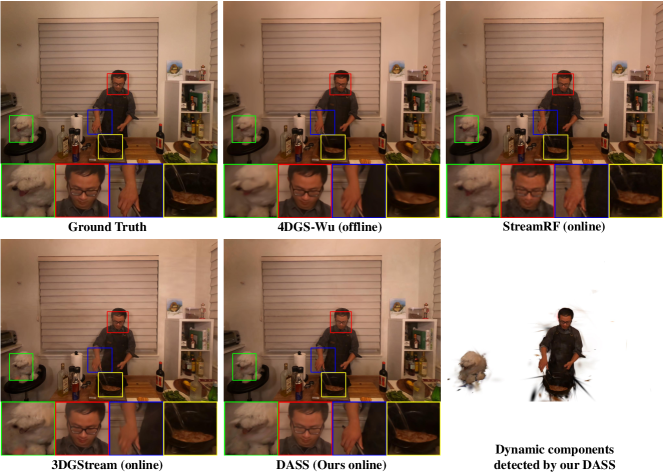
Figure 8: Qualitative results for the sear steak scene. Our method effectively captures the dramatic motions and color changes in the scene. However, the details in the furry dog part (green) and the steak part (yellow) are blurry in 4DGS-Wu, while the color of tongue (green) and the shape of hand (blue) are incorrect in 3DGStream.

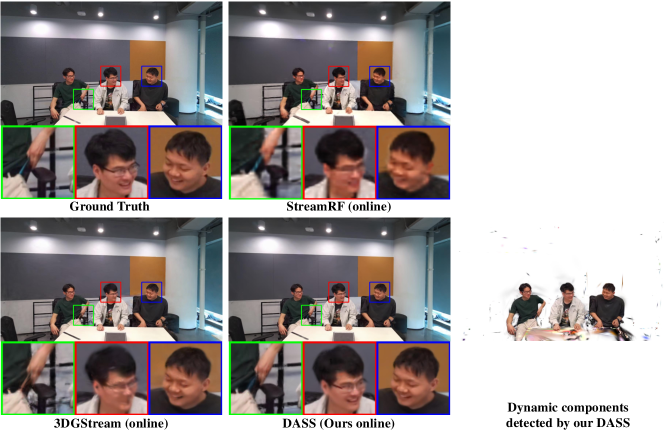
Figure 9: Qualitative results for the discussion scene. The baseline methods experience blurs and errors in dramatically dynamic areas, as seen in the hand moving out of the pocket (green) and in the human faces (red and blue). In contrast, our method preserves better dynamic features and motion representations. We implement 4DGS on the MeetRoom dataset but it fails to yield reasonable reconstruction, probably due to the sparse view challenges in this dataset.

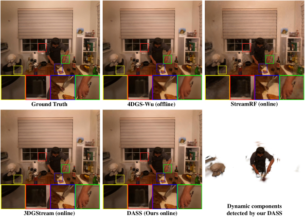
Figure 10: Qualitative results for the cut beef scene. The baselines 4DGS-Wu and StreamRF present over-smooth and lack some details (blue and green), while our DASS faithfully reconstructs finer details. Compared to 3DGStream, our DASS provides more accurate and vivid representations, such as the moving shadow (yellow), the reflection in the window (red), and the color of the knife (blue).

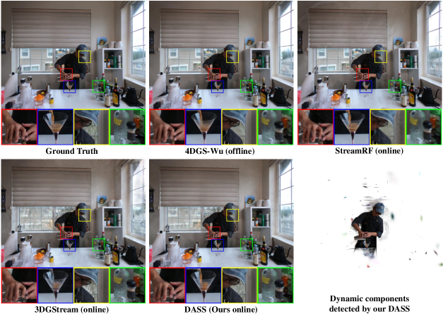
Figure 11: Qualitative results for the coffee martini scene. For 3DGStream, artifacts exist in the highly dynamic areas (red) and the coffee being poured is under-reconstructed (blue). While our DASS provides more accurate reconstructions in these challenging areas, it benefits from the fine reconstruction from the dynamics-aware shift and the inherited temporally continuous content that facilitates fast reconstruction of emerging objects. Besides, a loss of detail is observed (yellow and green) in baselines 4DGS-Wu and StreamRF. The reconstruction quality in the window area is relatively weak, since reconstructing distant components out of the window from COLMAP point clouds is difficult, which has been a longstanding challenge for general 3DGS-based methods.

References

- Arena et al. [2022] Fabio Arena, Mario Collotta, Giovanni Pau, and Francesco Termine. An overview of augmented reality. Computers, 11(2):28, 2022.
- Attal et al. [2023] Benjamin Attal, Jia-Bin Huang, Christian Richardt, Michael Zollhoefer, Johannes Kopf, Matthew O’Toole, and Changil Kim. Hyperreel: High-fidelity 6-dof video with ray-conditioned sampling. In Proceedings of the IEEE/CVF Conference on Computer Vision and Pattern Recognition, pages 16610–16620, 2023.
- Bae et al. [2024] Jeongmin Bae, Seoha Kim, Youngsik Yun, Hahyun Lee, Gun Bang, and Youngjung Uh. Per-Gaussian embedding-based deformation for deformable 3D Gaussian splatting. In European Conference on Computer Vision, 2024.
- Bengio et al. [2013] Yoshua Bengio, Nicholas Léonard, and Aaron Courville. Estimating or propagating gradients through stochastic neurons for conditional computation. arXiv preprint arXiv:1308.3432, 2013.
- Cao and Johnson [2023] Ang Cao and Justin Johnson. Hexplane: A fast representation for dynamic scenes. In Proceedings of the IEEE/CVF Conference on Computer Vision and Pattern Recognition, pages 130–141, 2023.
- Charatan et al. [2024] David Charatan, Sizhe Lester Li, Andrea Tagliasacchi, and Vincent Sitzmann. pixelsplat: 3D Gaussian splats from image pairs for scalable generalizable 3D reconstruction. In Proceedings of the IEEE/CVF Conference on Computer Vision and Pattern Recognition, pages 19457–19467, 2024.
- Chen et al. [2024a] Yiwen Chen, Zilong Chen, Chi Zhang, Feng Wang, Xiaofeng Yang, Yikai Wang, Zhongang Cai, Lei Yang, Huaping Liu, and Guosheng Lin. Gaussianeditor: Swift and controllable 3d editing with Gaussian splatting. In Proceedings of the IEEE/CVF Conference on Computer Vision and Pattern Recognition, pages 21476–21485, 2024a.
- Chen et al. [2024b] Yihang Chen, Qianyi Wu, Jianfei Cai, Mehrtash Harandi, and Weiyao Lin. HAC: Hash-grid assisted context for 3D Gaussian splatting compression. In European Conference on Computer Vision, 2024b.
- Cheng et al. [2023] Ho Kei Cheng, Seoung Wug Oh, Brian Price, Alexander Schwing, and Joon-Young Lee. Tracking anything with decoupled video segmentation. In Proceedings of the IEEE/CVF International Conference on Computer Vision, pages 1316–1326, 2023.
- Duan et al. [2024] Yuanxing Duan, Fangyin Wei, Qiyu Dai, Yuhang He, Wenzheng Chen, and Baoquan Chen. 4d-rotor gaussian splatting: towards efficient novel view synthesis for dynamic scenes. In ACM SIGGRAPH 2024 Conference Papers, pages 1–11, 2024.
- Fan et al. [2023] Zhiwen Fan, Kevin Wang, Kairun Wen, Zehao Zhu, Dejia Xu, and Zhangyang Wang. LightGaussian: Unbounded 3D Gaussian compression with 15x reduction and 200+ fps. arXiv preprint arXiv:2311.17245, 2023.
- Fridovich-Keil et al. [2022a] Sara Fridovich-Keil, Alex Yu, Matthew Tancik, Qinhong Chen, Benjamin Recht, and Angjoo Kanazawa. Plenoxels: Radiance fields without neural networks. In Proceedings of the IEEE/CVF Conference on Computer Vision and Pattern Recognition, pages 5501–5510, 2022a.
- Fridovich-Keil et al. [2022b] Sara Fridovich-Keil, Alex Yu, Matthew Tancik, Qinhong Chen, Benjamin Recht, and Angjoo Kanazawa. Plenoxels: Radiance fields without neural networks. In Proceedings of the IEEE/CVF conference on computer vision and pattern recognition, pages 5501–5510, 2022b.
- Fridovich-Keil et al. [2023] Sara Fridovich-Keil, Giacomo Meanti, Frederik Rahbæk Warburg, Benjamin Recht, and Angjoo Kanazawa. K-planes: Explicit radiance fields in space, time, and appearance. In Proceedings of the IEEE/CVF Conference on Computer Vision and Pattern Recognition, pages 12479–12488, 2023.
- Guo et al. [2024] Zhiyang Guo, Wengang Zhou, Li Li, Min Wang, and Houqiang Li. Motion-aware 3d Gaussian splatting for efficient dynamic scene reconstruction. arXiv preprint arXiv:2403.11447, 2024.
- He et al. [2024] Bing He, Yunuo Chen, Guo Lu, Li Song, and Wenjun Zhang. S4D: Streaming 4D real-world reconstruction with Gaussians and 3d control points. arXiv preprint arXiv:2408.13036, 2024.
- Hu et al. [2024] Yingdong Hu, Zhening Liu, Jiawei Shao, Zehong Lin, and Jun Zhang. Eva-Gaussian: 3D Gaussian-based real-time human novel view synthesis under diverse camera settings. arXiv preprint arXiv:2410.01425, 2024.
- Kajiya and Von Herzen [1984] James T Kajiya and Brian P Von Herzen. Ray tracing volume densities. ACM SIGGRAPH computer graphics, 18(3):165–174, 1984.
- Katsumata et al. [2024] Kai Katsumata, Duc Minh Vo, and Hideki Nakayama. A compact dynamic 3D Gaussian representation for real-time dynamic view synthesis. In European Conference on Computer Vision, 2024.
- Ke et al. [2024] Lei Ke, Mingqiao Ye, Martin Danelljan, Yu-Wing Tai, Chi-Keung Tang, Fisher Yu, et al. Segment anything in high quality. Advances in Neural Information Processing Systems, 36, 2024.
- Kerbl et al. [2023] Bernhard Kerbl, Georgios Kopanas, Thomas Leimkuehler, and George Drettakis. 3D Gaussian splatting for real-time radiance field rendering. ACM Transactions on Graphics (TOG), 42(4):1–14, 2023.
- Kheradmand et al. [2024] Shakiba Kheradmand, Daniel Rebain, Gopal Sharma, Weiwei Sun, Jeff Tseng, Hossam Isack, Abhishek Kar, Andrea Tagliasacchi, and Kwang Moo Yi. 3D Gaussian splatting as markov chain monte carlo. arXiv preprint arXiv:2404.09591, 2024.
- Kirillov et al. [2023] Alexander Kirillov, Eric Mintun, Nikhila Ravi, Hanzi Mao, Chloe Rolland, Laura Gustafson, Tete Xiao, Spencer Whitehead, Alexander C Berg, Wan-Yen Lo, et al. Segment anything. In Proceedings of the IEEE/CVF International Conference on Computer Vision, pages 4015–4026, 2023.
- Lee et al. [2024] Joo Chan Lee, Daniel Rho, Xiangyu Sun, Jong Hwan Ko, and Eunbyung Park. Compact 3D Gaussian representation for radiance field. In Proceedings of the IEEE/CVF Conference on Computer Vision and Pattern Recognition, pages 21719–21728, 2024.
- Li et al. [2022a] Lingzhi Li, Zhen Shen, Zhongshu Wang, Li Shen, and Ping Tan. Streaming radiance fields for 3D video synthesis. Advances in Neural Information Processing Systems, 35:13485–13498, 2022a.
- Li et al. [2022b] Tianye Li, Mira Slavcheva, Michael Zollhoefer, Simon Green, Christoph Lassner, Changil Kim, Tanner Schmidt, Steven Lovegrove, Michael Goesele, Richard Newcombe, et al. Neural 3D video synthesis from multi-view video. In Proceedings of the IEEE/CVF Conference on Computer Vision and Pattern Recognition, pages 5521–5531, 2022b.
- Li et al. [2024] Zhan Li, Zhang Chen, Zhong Li, and Yi Xu. Spacetime Gaussian feature splatting for real-time dynamic view synthesis. In Proceedings of the IEEE/CVF Conference on Computer Vision and Pattern Recognition, pages 8508–8520, 2024.
- Liu and Banerjee [2024] Bangya Liu and Suman Banerjee. Swings: Sliding window Gaussian splatting for volumetric video streaming with arbitrary length. arXiv preprint arXiv:2409.07759, 2024.
- Liu et al. [2025] Tianqi Liu, Guangcong Wang, Shoukang Hu, Liao Shen, Xinyi Ye, Yuhang Zang, Zhiguo Cao, Wei Li, and Ziwei Liu. MvsGaussian: Fast generalizable Gaussian splatting reconstruction from multi-view stereo. In European Conference on Computer Vision, pages 37–53. Springer, 2025.
- Liu et al. [2024] Xiangrui Liu, Xinju Wu, Pingping Zhang, Shiqi Wang, Zhu Li, and Sam Kwong. CompGS: Efficient 3D scene representation via compressed Gaussian splatting. arXiv preprint arXiv:2404.09458, 2024.
- Lu et al. [2024a] Tao Lu, Mulin Yu, Linning Xu, Yuanbo Xiangli, Limin Wang, Dahua Lin, and Bo Dai. Scaffold-GS: Structured 3D Gaussians for view-adaptive rendering. In Proceedings of the IEEE/CVF Conference on Computer Vision and Pattern Recognition, pages 20654–20664, 2024a.
- Lu et al. [2024b] Zhicheng Lu, Xiang Guo, Le Hui, Tianrui Chen, Min Yang, Xiao Tang, Feng Zhu, and Yuchao Dai. 3D geometry-aware deformable Gaussian splatting for dynamic view synthesis. In Proceedings of the IEEE/CVF Conference on Computer Vision and Pattern Recognition, pages 8900–8910, 2024b.
- Mildenhall et al. [2021] Ben Mildenhall, Pratul P Srinivasan, Matthew Tancik, Jonathan T Barron, Ravi Ramamoorthi, and Ren Ng. NeRF: Representing scenes as neural radiance fields for view synthesis. Communications of the ACM, 65(1):99–106, 2021.
- Müller et al. [2022] Thomas Müller, Alex Evans, Christoph Schied, and Alexander Keller. Instant neural graphics primitives with a multiresolution hash encoding. ACM transactions on graphics (TOG), 41(4):1–15, 2022.
- Pumarola et al. [2021] Albert Pumarola, Enric Corona, Gerard Pons-Moll, and Francesc Moreno-Noguer. D-NeRF: Neural radiance fields for dynamic scenes. In Proceedings of the IEEE/CVF Conference on Computer Vision and Pattern Recognition, pages 10318–10327, 2021.
- Shen et al. [2025] Qiuhong Shen, Xingyi Yang, and Xinchao Wang. Flashsplat: 2D to 3D Gaussian splatting segmentation solved optimally. In European Conference on Computer Vision, pages 456–472. Springer, 2025.
- Song et al. [2023] Liangchen Song, Anpei Chen, Zhong Li, Zhang Chen, Lele Chen, Junsong Yuan, Yi Xu, and Andreas Geiger. NeRFplayer: A streamable dynamic scene representation with decomposed neural radiance fields. IEEE Transactions on Visualization and Computer Graphics, 29(5):2732–2742, 2023.
- Sun et al. [2024a] Jiakai Sun, Han Jiao, Guangyuan Li, Zhanjie Zhang, Lei Zhao, and Wei Xing. 3DGStream: On-the-fly training of 3D Gaussians for efficient streaming of photo-realistic free-viewpoint videos. In Proceedings of the IEEE/CVF Conference on Computer Vision and Pattern Recognition, pages 20675–20685, 2024a.
- Sun et al. [2024b] Yuan-Chun Sun, Yuang Shi, Wei Tsang Ooi, Chun-Ying Huang, and Cheng-Hsin Hsu. Multi-frame bitrate allocation of dynamic 3D Gaussian splatting streaming over dynamic networks. In Proceedings of the 2024 SIGCOMM Workshop on Emerging Multimedia Systems, pages 1–7, 2024b.
- Teed and Deng [2020] Zachary Teed and Jia Deng. Raft: Recurrent all-pairs field transforms for optical flow. In Computer Vision–ECCV 2020: 16th European Conference, Glasgow, UK, August 23–28, 2020, Proceedings, Part II 16, pages 402–419. Springer, 2020.
- Tu et al. [2024] Hanzhang Tu, Ruizhi Shao, Xue Dong, Shunyuan Zheng, Hao Zhang, Lili Chen, Meili Wang, Wenyu Li, Siyan Ma, Shengping Zhang, et al. Tele-Aloha: A telepresence system with low-budget and high-authenticity using sparse rgb cameras. In ACM SIGGRAPH 2024 Conference Papers, pages 1–12, 2024.
- Wang et al. [2023] Feng Wang, Sinan Tan, Xinghang Li, Zeyue Tian, Yafei Song, and Huaping Liu. Mixed neural voxels for fast multi-view video synthesis. In Proceedings of the IEEE/CVF International Conference on Computer Vision, pages 19706–19716, 2023.
- Wang et al. [2024a] Penghao Wang, Zhirui Zhang, Liao Wang, Kaixin Yao, Siyuan Xie, Jingyi Yu, Minye Wu, and Lan Xu. V^ 3: Viewing volumetric videos on mobiles via streamable 2d dynamic Gaussians. arXiv preprint arXiv:2409.13648, 2024a.
- Wang et al. [2024b] Yuxin Wang, Qianyi Wu, Guofeng Zhang, and Dan Xu. GScream: Learning 3D geometry and feature consistent Gaussian splatting for object removal. arXiv preprint arXiv:2404.13679, 2024b.
- Wang et al. [2025] Yihan Wang, Lahav Lipson, and Jia Deng. Sea-raft: Simple, efficient, accurate raft for optical flow. In European Conference on Computer Vision, pages 36–54. Springer, 2025.
- Wang et al. [2003] Zhou Wang, Eero P Simoncelli, and Alan C Bovik. Multiscale structural similarity for image quality assessment. In The Thrity-Seventh Asilomar Conference on Signals, Systems & Computers, 2003, pages 1398–1402. Ieee, 2003.
- Wu et al. [2024] Guanjun Wu, Taoran Yi, Jiemin Fang, Lingxi Xie, Xiaopeng Zhang, Wei Wei, Wenyu Liu, Qi Tian, and Xinggang Wang. 4D Gaussian splatting for real-time dynamic scene rendering. In Proceedings of the IEEE/CVF Conference on Computer Vision and Pattern Recognition, pages 20310–20320, 2024.
- Xu et al. [2022a] Haofei Xu, Jing Zhang, Jianfei Cai, Hamid Rezatofighi, and Dacheng Tao. Gmflow: Learning optical flow via global matching. In Proceedings of the IEEE/CVF conference on computer vision and pattern recognition, pages 8121–8130, 2022a.
- Xu et al. [2023] Haofei Xu, Jing Zhang, Jianfei Cai, Hamid Rezatofighi, Fisher Yu, Dacheng Tao, and Andreas Geiger. Unifying flow, stereo and depth estimation. IEEE Transactions on Pattern Analysis and Machine Intelligence, 2023.
- Xu et al. [2022b] Qiangeng Xu, Zexiang Xu, Julien Philip, Sai Bi, Zhixin Shu, Kalyan Sunkavalli, and Ulrich Neumann. Point-NeRF: Point-based neural radiance fields. In Proceedings of the IEEE/CVF conference on computer vision and pattern recognition, pages 5438–5448, 2022b.
- Yang et al. [2024a] Ziyi Yang, Xinyu Gao, Wen Zhou, Shaohui Jiao, Yuqing Zhang, and Xiaogang Jin. Deformable 3D Gaussians for high-fidelity monocular dynamic scene reconstruction. In Proceedings of the IEEE/CVF Conference on Computer Vision and Pattern Recognition, pages 20331–20341, 2024a.
- Yang et al. [2024b] Zeyu Yang, Hongye Yang, Zijie Pan, and Li Zhang. Real-time photorealistic dynamic scene representation and rendering with 4D Gaussian splatting. In The Twelfth International Conference on Learning Representations, 2024b.
- Ye et al. [2025] Mingqiao Ye, Martin Danelljan, Fisher Yu, and Lei Ke. Gaussian grouping: Segment and edit anything in 3d scenes. In European Conference on Computer Vision, pages 162–179. Springer, 2025.
- Zhang et al. [2024] Xinjie Zhang, Zhening Liu, Yifan Zhang, Xingtong Ge, Dailan He, Tongda Xu, Yan Wang, Zehong Lin, Shuicheng Yan, and Jun Zhang. Mega: Memory-efficient 4D Gaussian splatting for dynamic scenes. arXiv preprint arXiv:2410.13613, 2024.
- Zhang et al. [2025] Xinjie Zhang, Xingtong Ge, Tongda Xu, Dailan He, Yan Wang, Hongwei Qin, Guo Lu, Jing Geng, and Jun Zhang. Gaussianimage: 1000 fps image representation and compression by 2D Gaussian splatting. In European Conference on Computer Vision, pages 327–345. Springer, 2025.
- Zheng et al. [2024] Shunyuan Zheng, Boyao Zhou, Ruizhi Shao, Boning Liu, Shengping Zhang, Liqiang Nie, and Yebin Liu. Gps-Gaussian: Generalizable pixel-wise 3D Gaussian splatting for real-time human novel view synthesis. In Proceedings of the IEEE/CVF Conference on Computer Vision and Pattern Recognition, pages 19680–19690, 2024.
- Zwicker et al. [2001] Matthias Zwicker, Hanspeter Pfister, Jeroen Van Baar, and Markus Gross. EWA volume splatting. In Proceedings Visualization, 2001. VIS’01., pages 29–538. IEEE, 2001.