theorempropositiondefinitioncorollarylemmaquote

Entropic Fluctuation Theorems for the Spin–Fermion Model

Abstract. We study entropic fluctuations in the Spin–Fermion model describing an $N$-level quantum system coupled to several independent thermal free Fermi gas reservoirs. We establish the quantum Evans–Searles and Gallavotti–Cohen fluctuation theorems and identify their link with entropic ancilla state tomography and quantum phase space contraction of non-equilibrium steady state. The method of proof involves the spectral resonance theory of quantum transfer operators developed by the authors in previous works.

1 Introduction

This is the fourth and final paper in a series [BBJ⁺24b, BBJ⁺25, BBJ⁺24a] dealing with entropic fluctuations in quantum statistical mechanics, and in particular with the quantum Evans–Searles and Gallavotti–Cohen fluctuation theorems. Its goal is to illustrate, on the example of the open spin–fermion model, the general theory developed in [BBJ⁺24b, BBJ⁺24a]. The work [BBJ⁺25] was devoted to the justification of the key formulas of [BBJ⁺24b] by thermodynamic limit arguments.

We assume the reader to be familiar with the framework and results of [BBJ⁺24b, BBJ⁺25, BBJ⁺24a]. In particular, we will use the notation and conventions regarding open quantum systems and modular theory introduced in these works.

In the context of open quantum systems, the spin–fermion model goes back to the works [Dav74, SL78], and with time has become one of the paradigmatic models of quantum statistical mechanics. The closely related spin–boson model, in which each thermal reservoir is a free Bose gas, has a much longer history in the physics literature due to its connection with non-relativistic QED; see e.g. [DJ01, Section 1.6]. The description and analysis of the spin–boson model is technically more involved, and the model does not fit directly in the $C^{\ast}$-algebraic formalism of [BBJ⁺24b, BBJ⁺24a].

The revival of interest in the spin–fermion/boson model started with [JP96a, JP96b, BFS98] that have generated a large body of literature; an incomplete list of references is [HS95, DG99, BFS00, DJ01, Mer01, FGS02, JP02, DJ03, FM04, JOP06, MMS07, AS07, DDR08, DR09, DRK13, Mø14, HHS21]. We will comment on some of these works as we proceed. The techniques we will use draw on [JP96a, JP96b, JP02, JOPP10].

The paper is organized as follows. In Section 2, we introduce the spin–fermion model, briefly recall the main objects of study and state our results. In Section 3, for the convenience of the reader, we recall the modular structure of the model, as well as the $\alpha$-Liouvilleans introduced in [JOPP10, BBJ⁺24a] and their connection with the various entropic functionals. Section 4 is devoted to the study of these $\alpha$-Liouvilleans and closely follows the analysis in [JP96a, JP96b, JP02]. The proof of the main theorem is given in Section 5.

Acknowledgments

The work of CAP and VJ was partly funded by the CY Initiative grant Investissements d’Avenir, grant number ANR-16-IDEX-0008. The work of TB was funded by the ANR project ESQuisses, grant number ANR-20-CE47-0014-01, and by the ANR project Quantum Trajectories, grant number ANR-20-CE40-0024-01. VJ acknowledges the support of NSERC. A part of this work was done during long term visits of LB and AP to McGill and CRM–CNRS International Research Laboratory IRL 3457 at University of Montreal. The LB visit was funded by the CNRS and AP visits by the CRM Simons and FRQNT–CRM–CNRS programs. We also acknowledge the support of the ANR project DYNACQUS, grant number ANR-24-CE40-5714.

2 The Spin–Fermion Model

2.1 Description of the model

The spin–fermion model is a concrete example of open quantum system with the structure described in [BBJ⁺24b, Section 1.1], where several independent reservoirs are coupled through a small system $\mathsf{S}$. The model has a non-trivial small system part, described by a finite dimensional Hilbert space $\mathcal{K}_{\mathsf{S}}$ and Hamiltonian $H_{\mathsf{S}}$. Its $C^{\ast}$-algebra of observables is $\mathcal{O}_{\mathsf{S}}=\mathcal{B}(\mathcal{K}_{\mathsf{S}})$, where $\mathcal{B}(\mathcal{H})$ denotes the $C^{\ast}$-algebra of all bounded operators on a Hilbert space $\mathcal{H}$. Its dynamics $\tau_{\mathsf{S}}^{t}=\mathrm{e}^{t\delta_{\mathsf{S}}}$ is generated by $\delta_{\mathsf{S}}=\mathrm{i}[H_{\mathsf{S}},\,\cdot\;]$ and its reference state is $\omega_{\mathsf{S}}(A)=\mathop{\mathrm{tr}}\nolimits(A)/\mathop{\mathrm{dim}}\,\mathcal{K}_{\mathsf{S}}$. Each reservoir subsystem $\mathsf{R}_{j}$, $1\leq j\leq M$, is a free Fermi gas with single particle Hilbert space $\mathfrak{h}_{j}$ and single particle Hamiltonian $h_{j}$. The algebra of observables of $\mathsf{R}_{j}$ is the CAR-algebra $\mathcal{O}_{j}=\mathop{\mathrm{CAR}}(\mathfrak{h}_{j})$, the $C^{\ast}$-algebra generated by creation/annihilation operators $a_{j}^{\ast}(f)$/$a_{j}(f)$, $f\in\mathfrak{h}_{j}$, satisfying the canonical anti-commutation relations

$$\{a_{j}(f),a_{j}^{\ast}(g)\}=\langle f,g\rangle\mathbb{1},\qquad\{a_{j}(f),a_{j}(g)\}=0.$$

The Heisenberg dynamics on $\mathcal{O}_{j}$ is the group of Bogoliubov $\ast$-automorphisms associated to $h_{j}$, i.e., the $C^{\ast}$-dynamics defined by $\tau_{j}^{t}(a_{j}(f))=a_{j}\left(\mathrm{e}^{\mathrm{i}th_{j}}f\right)$. We denote by $\delta_{j}$ its generator, $\tau_{j}^{t}=\mathrm{e}^{t\delta_{j}}$. The reference state $\omega_{j}$ on $\mathcal{O}_{j}$ is the gauge-invariant quasi-free state generated by the Fermi-Dirac density operator

$$T_{j}=\left(\mathbb{1}+\mathrm{e}^{\beta_{j}h_{j}}\right)^{-1},$$

where $\beta_{j}>0$ is the inverse temperature. $\omega_{j}$ is the unique $(\tau_{j},\beta_{j})$-KMS state on $\mathcal{O}_{j}$. The full reservoir system $\mathsf{R}=\mathsf{R}_{1}+\cdots+\mathsf{R}_{M}$ is described by the quantum dynamical system $(\mathcal{O}_{\mathsf{R}},\tau_{\mathsf{R}},\omega_{\mathsf{R}})$ where

$$\begin{split}\mathcal{O}_{\mathsf{R}}&=\mathcal{O}_{1}\otimes\cdots\otimes\mathcal{O}_{M},\\[2.84526pt] \tau_{\mathsf{R}}&=\tau_{1}\otimes\cdots\otimes\tau_{M},\\[2.84526pt] \omega_{\mathsf{R}}&=\omega_{1}\otimes\cdots\otimes\omega_{M}.\end{split}$$

The $C^{\ast}$-algebra and reference state of the joint system $\mathsf{S}+\mathsf{R}$ are $\mathcal{O}=\mathcal{O}_{\mathsf{S}}\otimes\mathcal{O}_{\mathsf{R}}$ and $\omega=\omega_{\mathsf{S}}\otimes\omega_{\mathsf{R}}$. In the absence of interaction between $\mathsf{S}$ and $\mathsf{R}$, its dynamics is $\tau_{\mathrm{fr}}=\tau_{\mathsf{S}}\otimes\tau_{\mathsf{R}}$. This free dynamics is generated by $\delta_{\mathrm{fr}}=\delta_{\mathsf{S}}+\delta_{1}+\cdots+\delta_{M}$.

For each $j$, the interaction of $\mathsf{S}$ with $\mathsf{R}_{j}$ is described by

$$V_{j}=\sum_{k=1}^{m_{j}}Q_{j,k}\otimes R_{j,k}\in\mathcal{O}_{\mathsf{S}}\otimes\mathcal{O}_{j},$$ (2.1)

where $Q_{j,k}\in\mathcal{O}_{\mathsf{S}}$ is self-adjoint and

$$R_{j,k}=\mathrm{i}^{n_{j,k}(n_{j,k}-1)/2}\varphi_{j}(f_{j,k,1})\cdots\varphi_{j}(f_{j,k,n_{j,k}}),$$ (2.2)

with form factors $f_{j,k,m}\in\mathfrak{h}_{j}$, and where $\varphi_{j}(f)=\frac{1}{\sqrt{2}}(a_{j}(f)+a_{j}^{\ast}(f))$ are the Segal field operators. Following [Dav74], we assume that:

(SFM0) For all $t\in\mathbb{R}$, $j\in\{1,\ldots,M\}$ and $(k,m)\not=(k^{\prime},m^{\prime})$,

$$\langle f_{j,k,m},\mathrm{e}^{\mathrm{i}th_{j}}f_{j,k^{\prime},m^{\prime}}\rangle=0.$$

In particular, taking $t=0$ in (SFM0) ensures that the $R_{j,k}$ are self-adjoint elements of $\mathcal{O}_{j}$.

Without further mentioning we will assume (SFM0) throughout the paper. The complete interaction is $V=\sum_{j}V_{j}$, and the interacting dynamics $\tau_{\lambda}$ is generated by

$$\delta=\delta_{\mathrm{fr}}+\lambda\mathrm{i}[V,\,\cdot\;],$$

where $\lambda\in\mathbb{R}$ is a coupling constant. The coupled system $\mathsf{S}+\mathsf{R}$ is described by the $C^{\ast}$-quantum dynamical system $(\mathcal{O},\tau_{\lambda},\omega)$. We denote by $\omega_{t}=\omega\circ\tau_{\lambda}^{t}$ the evolution of the state $\omega$ at time $t$.

Remark 2.1.

In the simplest and most studied example of spin–fermion model one has $\mathcal{K}_{\mathsf{S}}=\mathbb{C}^{2}$, $H_{\mathsf{S}}=\sigma_{z}$ and for each reservoir $\mathsf{R}_{j}$ the interaction is of the form $V_{j}=\sigma_{x}\otimes\varphi(f_{j})$, where $\sigma_{z}$ and $\sigma_{x}$ denote the usual Pauli matrices, see the example at the end of Section 2.4.

As already mentioned, we are interested in the quantum versions of both Evans–Searles and Gallavotti–Cohen fluctuation theorems, a convenient reference in the spirit of the present work is the review [JPRB11]. The former refers to entropic fluctuations with respect to the initial (reference) state $\omega$ of the system while the latter refers to these fluctuations with respect to the Non-Equilibrium Steady State (NESS) $\omega_{+}$ of the system. The next assumption postulates the existence of such an NESS of $(\mathcal{O},\tau_{\lambda},\omega)$.

(SFM1) For all $A\in\mathcal{O}$ the limit

$$\omega_{+}(A)=\lim_{t\uparrow\infty}\omega_{t}(A)$$

exists, and the restriction $\omega_{+\mathsf{S}}$ of the state $\omega_{+}$ to $\mathcal{O}_{\mathsf{S}}$ is faithful, $\omega_{+\mathsf{S}}>0$.

In Section 2.4 we will describe sufficient conditions that guarantee the validity of (SFM1).

A time reversal of the $C^{\ast}$-dynamics $\tau_{\lambda}$ is an anti-linear involutive $\ast$-automorphism $\Theta$ of $\mathcal{O}$ such that $\Theta\circ\tau_{\lambda}^{t}=\tau_{\lambda}^{-t}\circ\Theta$ for all $t\in\mathbb{R}$. A state $\nu$ on $(\mathcal{O},\tau_{\lambda})$ is time-reversal invariant if $\tau_{\lambda}$ admits a time reversal $\Theta$ such that $\nu\circ\Theta(A)=\nu(A^{\ast})$ for all $A\in\mathcal{O}$. In this case, we will say that the quantum dynamical system $(\mathcal{O},\tau_{\lambda},\nu)$ is time-reversal invariant (TRI).

If $(\mathcal{O},\tau_{\lambda},\omega)$ is TRI, then (SFM1) implies that for all $A\in\mathcal{O}$ the limit

$$\omega_{-}(A)=\lim_{t\to-\infty}\omega_{t}(A)$$

exists, and is given by $\omega_{-}(A)=\omega_{+}\circ\Theta(A^{\ast})$.

2.2 Entropy production and entropic functionals

Before introducing the three entropic functionals which are the main objects of our study, we briefly recall the mathematical framework needed to define these objects. The purpose here is to fix our notation, and we must refer the reader to [BBJ⁺24b, BBJ⁺24a] for a more detailed introduction and discussions.

Let $(\mathcal{H},\pi,\Omega)$ be the GNS-representation of $\mathcal{O}$ induced by $\omega$. The enveloping algebra $\mathfrak{M}$ is the smallest von Neumann subalgebra of $\mathcal{B}(\mathcal{H})$ containing $\pi(\mathcal{O})$. A state on $\mathfrak{M}$ is normal whenever it is described by a density matrix on $\mathcal{H}$. The states on $\mathcal{O}$ obtained as restrictions of these normal states are called $\omega$-normal and form the folium $\mathcal{N}$ of $\omega$.

The dynamical system $(\mathcal{O},\tau_{\lambda},\omega)$ is modular: $\omega$ is a $(\varsigma_{\omega},-1)$-KMS state where $\varsigma_{\omega}^{t}=\mathrm{e}^{t\delta_{\omega}}$, the modular group of $\omega$, is the $C^{\ast}$-dynamics generated by

$$\delta_{\omega}=-\sum_{j=1}^{M}\beta_{j}\delta_{j}.$$

Since $\delta_{j}(\varphi_{j}(f))=\varphi_{j}(\mathrm{i}h_{j}f)$, our next assumption ensures that $V_{j}\in\mathop{\mathrm{Dom}}(\delta_{j})$, and hence $V\in\mathop{\mathrm{Dom}}(\delta_{\omega})$.

(SFM2) $f_{j,k,m}\in\mathop{\mathrm{Dom}}(h_{j})$ for all $j,k,m$.

The observable $\Phi_{j}=-\lambda\delta_{j}(V_{j})$ is then well-defined, and describes the energy flux out of the $j^{\text{th}}$ reservoir. This brings us to the notion of entropy production rate, given by the observable [JP01, Rue01]

$$\sigma=\lambda\delta_{\omega}(V)=\sum_{j=1}^{M}\beta_{j}\Phi_{j},$$

satisfying the entropy balance relation, see e.g. [JP01],

$$\mathop{\mathrm{Ent}}(\omega_{t}|\omega)=-\int_{0}^{t}\omega_{s}(\sigma)\mathrm{d}s.$$ (2.3)

The left-hand side of this relation is Araki’s relative entropy [Ara76, Ara77], with the sign and ordering convention of [JP01]. Since this quantity is non-positive, one has $\int_{0}^{t}\omega_{s}(\sigma)\mathrm{d}s\geq 0$ for all $t\in\mathbb{R}$, and hence $\omega_{+}(\sigma)\geq 0$.

Remark 2.2.

Whenever $\Theta$ is a time reversal for $\tau_{\lambda}$, irrespective of the coupling $\lambda\in\mathbb{R}$, then $\Theta(V)=V$ and $\Theta(\sigma)=-\sigma$, so that $\omega_{-}(\sigma)\leq 0$. In particular, $\omega_{+}(\sigma)=0$ if $\omega_{-}=\omega_{+}$.

For $\alpha\in\mathrm{i}\mathbb{R}$, the Connes cocycle of a pair $(\mu,\nu)$ of faithful $\omega$-normal states is

$$[D\mu:D\nu]_{\alpha}=\Delta_{\mu|\nu}^{\alpha}\Delta_{\nu}^{-\alpha},$$

where $\Delta_{\nu}$, the modular operator of the state $\nu$, and $\Delta_{\mu|\nu}$, the relative modular operator of the pair $(\mu,\nu)$, are both non-negative operators on $\mathcal{H}$. Thus, $([D\mu:D\nu]_{\alpha})_{\alpha\in\mathrm{i}\mathbb{R}}$ is a family of unitaries on $\mathcal{H}$ which, in fact, belong to $\mathfrak{M}$, see e.g. [AM82, Appendix B]. We further have

Proposition 2.3.

Suppose (SFM2) holds. Then, for all $t\in\mathbb{R}$, $([D\omega_{t}:D\omega]_{\alpha})_{\alpha\in\mathrm{i}\mathbb{R}}\subset\pi(\mathcal{O})$.

In what follows we write $[D\omega_{t}:D\omega]_{\alpha}$ for $\pi^{-1}([D\omega_{t}:D\omega]_{\alpha})$. Similarly, whenever the meaning is clear within the context, we write $A$ for $\pi(A)$. The proof of the above proposition relies on the identity

$$\log\Delta_{\omega_{t}|\omega}=\log\Delta_{\omega}+Q_{t},\qquad Q_{t}=\int_{0}^{t}\tau_{\lambda}^{-s}(\sigma)\mathrm{d}s,$$ (2.4)

and the subsequent norm convergent expansion

$$[D\omega_{t}:D\omega]_{\alpha}=\mathbb{1}+\sum_{n\geq 1}\alpha^{n}\int\limits_{0\leq\theta_{1}\leq\cdots\leq\theta_{n}\leq 1}\varsigma_{\omega}^{-\mathrm{i}\theta_{1}\alpha}(Q_{t})\cdots\varsigma_{\omega}^{-\mathrm{i}\theta_{n}\alpha}(Q_{t})\mathrm{d}\theta_{1}\cdots\mathrm{d}\theta_{n}.$$ (2.5)

For more details about Relations (2.4)–(2.5), we refer the reader to [BBJ⁺25, Section 2], and in particular Lemma 2.4 and Equation (2.13) in this reference.

We can now introduce the three entropic functionals considered in [BBJ⁺24a]. We only briefly recall their definition and refer the reader to [BBJ⁺24b, BBJ⁺24a] for an in depth discussion.

Two-time measurement entropy production (2TMEP)

The following result was established in [BBJ⁺24b, Theorem 1.3]. For any $\nu\in\mathcal{N}$, $t\in\mathbb{R}$, and $\alpha\in\mathrm{i}\mathbb{R}$, the limit

$$\mathfrak{F}_{\nu,t}^{\mathrm{2tm}}(\alpha)=\lim_{R\to\infty}\frac{1}{R}\int_{0}^{R}\nu\circ\varsigma_{\omega}^{\theta}\left([D\omega_{-t}:D\omega]_{\alpha}\right)\mathrm{d}\theta$$

exists, and there is a unique Borel probability measure $Q_{\nu,t}^{\mathrm{2tm}}$ on $\mathbb{R}$ such that

$$\mathfrak{F}_{\nu,t}^{\mathrm{2tm}}(\alpha)=\int_{\mathbb{R}}\mathrm{e}^{-\alpha s}\mathrm{d}Q_{\nu,t}^{\mathrm{2tm}}(s).$$ (2.6)

Moreover, one also has that

$$\mathfrak{F}_{\nu,t}^{\mathrm{2tm}}(\alpha)=\lim_{R\to\infty}\frac{1}{R}\int_{0}^{R}\nu\circ\varsigma_{\omega}^{\theta}\left([D\omega_{-t}:D\omega]_{\frac{\bar{\alpha}}{2}}^{\ast}[D\omega_{-t}:D\omega]_{\frac{\alpha}{2}}\right)\mathrm{d}\theta.$$

As discussed in [BBJ⁺24b, BBJ⁺24a], the family $\left(Q_{\nu,t}^{\mathrm{2tm}}\right)_{t\in\mathbb{R}}$ describes the statistics of a two-time measurement of the entropy produced during a time period of length $t$ in the system $(\mathcal{O},\tau_{\lambda},\omega)$, when the latter is in the state $\nu$ at the time of the first measurement. In [BBJ⁺24b] it was also shown that, if each reservoir system $(\mathcal{O}_{j},\tau_{j},\omega_{j})$ is ergodic, then the map

$$\mathcal{N}\ni\nu\mapsto Q_{\nu,t}\in\mathcal{P}(\mathbb{R}),$$

where $\mathcal{P}(\mathbb{R})$ denotes the set of all Borel probability measures on $\mathbb{R}$ equipped with the weak topology, extends by continuity to the set $\mathcal{S}_{\mathcal{O}}$ of all states on $\mathcal{O}$, equipped with the weak^∗ topology. This defines $Q_{\nu,t}$, hence $\mathfrak{F}_{\nu,t}^{\mathrm{2tm}}$ by (2.6), for all $\nu\in\mathcal{S}_{\mathcal{O}}$. We will be particularly interested in the case $\nu=\omega_{+}$.

Entropic ancilla state tomography (EAST)

For $\nu\in\mathcal{S}_{\mathcal{O}}$, $t\in\mathbb{R}$ and $\alpha\in\mathrm{i}\mathbb{R}$, we set

$$\mathfrak{F}_{\nu,t}^{\mathrm{ancilla}}(\alpha)=\nu\left([D\omega_{-t}:D\omega]^{\ast}_{\frac{\bar{\alpha}}{2}}[D\omega_{-t}:D\omega]_{\frac{\alpha}{2}}\right).$$

EAST is described by the family of functionals $\left(\mathfrak{F}_{\nu,t}^{\mathrm{ancilla}}\right)_{t\in\mathbb{R}}$. When $\nu=\omega$, and up to an irrelevant prefactor, $\mathfrak{F}_{\omega,t}^{\mathrm{ancilla}}(\alpha)$ provides an experimental implementation of $\mathfrak{F}_{\omega,t}^{\mathrm{2tm}}(\alpha)$ through coupling and specific indirect projective measurements on an ancilla, a procedure called ancilla state tomography, see [BBJ⁺24a, Section 2.4] and references therein.

Quantum phase space contraction (QPSC)

For $\nu\in\mathcal{S}_{\mathcal{O}}$, $t\in\mathbb{R}$ and $\alpha\in\mathrm{i}\mathbb{R}$, we set

$$\mathfrak{F}_{\nu,t}^{\mathrm{qpsc}}(\alpha)=\nu\left([D\omega_{-t}:D\omega]_{\alpha}\right).$$

QPSC is described by the family of functionals $\left(\mathfrak{F}_{\nu,t}^{\mathrm{qpsc}}\right)_{t\in\mathbb{R}}$ and provides another natural route to the quantization of the classical entropic functionals [BBJ⁺24a, Section 2.7].

Note that when $\nu=\omega$ the three families of functionals coincide,

$$\mathfrak{F}_{\omega,t}^{\mathrm{2tm}}=\mathfrak{F}_{\omega,t}^{\mathrm{ancilla}}=\mathfrak{F}_{\omega,t}^{\mathrm{qpsc}},$$ (2.7)

and that

$$\partial_{\alpha}\mathfrak{F}_{\omega,t}^{\mathrm{2tm}}(\alpha)\big{|}_{\alpha=0}=-\int_{\mathbb{R}}s\,\mathrm{d}Q_{\omega,t}^{\mathrm{2tm}}(s)=\mathop{\mathrm{Ent}}(\omega_{t}|\omega).$$ (2.8)

The equalities (2.7) are however broken if $\omega$ is replaced by some other state $\nu\in\mathcal{S}_{\mathcal{O}}$.

2.3 Fluctuation theorems and the principle of regular entropic fluctuations

We first strengthen (SFM2) to

(SFM3) $f_{j,k,m}\in\mathop{\mathrm{Dom}}\left(\mathrm{e}^{a|h_{j}|}\right)$ for all $a>0$ and all $j,k,m$.

Since $\varsigma_{\omega}^{\theta}(\varphi_{j}(f))=\varphi\left(\mathrm{e}^{-\mathrm{i}\theta\beta_{j}h_{j}}f\right)$, Assumption (SFM3) guarantees that $V$ is an entire element for the modular group $\varsigma_{\omega}$, so that the regularity assumption (AnV$\boldsymbol{(\vartheta)}$) of [BBJ⁺24a] is satisfied for any $\vartheta>0$.

Our next assumption ensures that all the reservoir subsystems $(\mathcal{O}_{j},\tau_{j},\omega_{j})$ are ergodic. As a consequence, the probability distribution $Q_{\omega_{+},t}^{\mathrm{2tm}}$ and entropic functional $\mathfrak{F}^{\mathrm{2tm}}_{\omega_{+},t}$ are well-defined.

(SFM4) $h_{j}$ has purely absolutely continuous spectrum for all $j$.

The last two assumptions have the following consequence

Theorem 2.4.

Suppose that (SFM1), (SFM3) and (SFM4) hold. Then, for all $t\in\mathbb{R}$:

1. The map

   $$\mathrm{i}\mathbb{R}\ni\alpha\mapsto[D\omega_{t}:D\omega]_{\alpha}\in\mathcal{O}$$

   extends to an entire analytic function.

2. The maps

   $$\begin{split}\alpha&\mapsto\mathfrak{F}_{\omega,t}^{\mathrm{2tm}}(\alpha),\\[2.84526pt] \alpha&\mapsto\mathfrak{F}_{\omega_{+},t}^{\mathrm{2tm}}(\alpha),\\[2.84526pt] \alpha&\mapsto\mathfrak{F}_{\omega_{+},t}^{\mathrm{ancilla}}(\alpha),\\[2.84526pt] \alpha&\mapsto\mathfrak{F}_{\omega_{+},t}^{\mathrm{qpsc}}(\alpha),\end{split}$$

   defined for $\alpha\in\mathrm{i}\mathbb{R}$, extend to entire analytic functions. Moreover, for all $\alpha\in\mathbb{C}$,

   $$\mathfrak{F}_{\omega,t}^{\mathrm{2tm}}(\alpha)=\int_{\mathbb{R}}\mathrm{e}^{-\alpha s}\mathrm{d}Q_{\omega,t}^{\mathrm{2tm}}(s),\qquad\mathfrak{F}_{\omega_{+},t}^{\mathrm{2tm}}(\alpha)=\int_{\mathbb{R}}\mathrm{e}^{-\alpha s}\mathrm{d}Q_{\omega_{+},t}^{\mathrm{2tm}}(s).$$

3. The measures $Q_{\omega,t}^{\mathrm{2tm}}$ and $Q_{\omega_{+},t}^{\mathrm{2tm}}$ are equivalent, and for some constants $k,K>0$ and all $t\in\mathbb{R}$,

   $$k\leq\frac{\mathrm{d}Q_{\omega_{+},t}^{\mathrm{2tm}}}{\mathrm{d}Q_{\omega,t}^{\mathrm{2tm}}}\leq K.$$

Proof.

Part (1) follows from (SFM3) and [BBJ⁺24a, Proposition 2.11] while Part (2) is a consequence of (SFM1)+(SFM3), [BBJ⁺24a, Proposition 3.2] and a well known property of Laplace transforms. Finally, Part (3) follows from (SFM4) and [BBJ⁺24b, Theorem 1.6].

Assuming that (SFM1)–(SFM4) hold, we are now ready to introduce the principle of regular entropic fluctuations (abbreviated the PREF) of [BBJ⁺24a]. There, the PREF was introduced in several forms: weak, strong, and strong + qpsc. Here we will deal only with the latest (and strongest) form, and therefore we drop its qualification.

Definition 2.5.

Let $I=\,]\vartheta_{-},\vartheta_{+}[$ be an open interval containing $0$. We say that $(\mathcal{O},\tau_{\lambda},\omega)$ satisfies the PREF on the interval $I$ if, for all $\alpha\in I$, the limits

$$\begin{split}\boldsymbol{F}^{\mathrm{2tm}}_{\omega}(\alpha)&=\lim_{t\to\infty}\frac{1}{t}\log\mathfrak{F}_{\omega,t}^{\mathrm{2tm}}(\alpha),\\[2.84526pt] \boldsymbol{F}^{\mathrm{2tm}}_{\omega_{+}}(\alpha)&=\lim_{t\to\infty}\frac{1}{t}\log\mathfrak{F}_{\omega_{+},t}^{\mathrm{2tm}}(\alpha),\\[2.84526pt] \boldsymbol{F}^{\mathrm{ancilla}}_{\omega_{+}}(\alpha)&=\lim_{t\to\infty}\frac{1}{t}\log\mathfrak{F}^{\mathrm{ancilla}}_{\omega_{+},t}(\alpha),\\[2.84526pt] \boldsymbol{F}^{\mathrm{qpsc}}_{\omega_{+}}(\alpha)&=\lim_{t\to\infty}\frac{1}{t}\log\mathfrak{F}^{\mathrm{qpsc}}_{\omega_{+},t}(\alpha)\end{split}$$ (2.9)

exist, and define differentiable functions on $I$, satisfying

$$\boldsymbol{F}^{\mathrm{2tm}}_{\omega}=\boldsymbol{F}^{\mathrm{2tm}}_{\omega_{+}}=\boldsymbol{F}^{\rm ancilla}_{\omega_{+}}=\boldsymbol{F}^{\mathrm{qpsc}}_{\omega_{+}}.$$ (2.10)

We denote by $\boldsymbol{F}$ the common function in (2.10).

Remark 2.6.

While $\mathfrak{F}_{\omega,t}^{\mathrm{2tm}}(\alpha)$, $\mathfrak{F}_{\omega_{+},t}^{\mathrm{2tm}}(\alpha)$ and $\mathfrak{F}_{\omega_{+},t}^{\mathrm{ancilla}}(\alpha)$ are obviously positive for $\alpha\in\mathbb{R}$, the quantity $\mathfrak{F}_{\omega_{+},t}^{\mathrm{qpsc}}(\alpha)$ is a priori complex. The principal branch of the logarithm should be understood in the definition of $\boldsymbol{F}^{\mathrm{qpsc}}_{\omega_{+}}$. This makes $\log\mathfrak{F}^{\mathrm{qpsc}}_{\omega_{+},t}(\alpha)$ well-defined for $\lambda$ small enough and $t$ large, see (5.8) and Remark 5.6.

Definition 2.5 has several aspects. By the Gärtner-Ellis theorem, the existence and differentiability of the first limit in (2.9) give that the family of measures $\left(Q_{\omega,t}^{\mathrm{2tm}}(t\,\cdot\;)\right)_{t>0}\subset\mathcal{P}(\mathbb{R})$ satisfies a large deviation principle on the interval $]a,b[$, where $]a,b[\,=\mathbb{R}$ if $I=\mathbb{R}$, and otherwise

$$a=\lim_{\alpha\downarrow\vartheta_{-}}\partial_{\alpha}\boldsymbol{F}_{\omega}^{\mathrm{2tm}}(\alpha),\qquad b=\lim_{\alpha\uparrow\vartheta_{+}}\partial_{\alpha}\boldsymbol{F}_{\omega}^{\mathrm{2tm}}(\alpha),$$

with the rate function

$$\mathbb{I}(s)=\sup_{-\alpha\in I}(s\alpha-\boldsymbol{F}_{\omega}^{\mathrm{2tm}}(-\alpha)).$$

This is the quantum Evans–Searles fluctuation theorem. When the system is TRI one moreover has $\mathfrak{F}_{\omega,t}^{\mathrm{2tm}}(\alpha)=\mathfrak{F}_{\omega,t}^{\mathrm{2tm}}(1-\alpha)$ for all real $\alpha$ and all $t$, see [BBJ⁺24b, Theorem 1.4]. This leads to the celebrated symmetry

$${\mathbb{I}}(-s)=s+{\mathbb{I}}(s),$$ (2.11)

called the quantum Evans–Searles fluctuation relation, that holds for $|s|<\min\{-a,b\}$, see [BBJ⁺24a, Proposition 2.6].

The existence and differentiability of the second limit in (2.9) give that $\left(Q_{\omega_{+},t}^{\mathrm{2tm}}(t\,\cdot\;)\right)_{t>0}\subset\mathcal{P}(\mathbb{R})$ satisfies a large deviation principle on the interval $]a_{+},b_{+}[$, where $]a_{+},b_{+}[\,=\mathbb{R}$ if $I=\mathbb{R}$, and otherwise

$$a_{+}=\lim_{\alpha\downarrow\vartheta_{-}}\partial_{\alpha}\boldsymbol{F}_{\omega_{+}}^{\mathrm{2tm}}(\alpha),\qquad b_{+}=\lim_{\alpha\uparrow\vartheta_{+}}\partial_{\alpha}\boldsymbol{F}_{\omega_{+}}^{\mathrm{2tm}}(\alpha),$$

with the rate function

$$\mathbb{I}_{+}(s)=\sup_{-\alpha\in I}(s\alpha-\boldsymbol{F}^{\mathrm{2tm}}_{\omega_{+}}(-\alpha)).$$

This is the quantum Gallavotti–Cohen fluctuation theorem. Theorem 2.4(3) identifies these two fluctuation theorems: $\boldsymbol{F}^{\mathrm{2tm}}_{\omega_{+}}=\boldsymbol{F}^{\mathrm{2tm}}_{\omega}$, $a=a_{+}$, $b=b_{+}$, $\mathbb{I}=\mathbb{I}_{+}$. If the system is TRI, the symmetry $\mathbb{I}_{+}(-s)=s+\mathbb{I}_{+}(s)$ therefore also holds. This is the quantum Gallavotti–Cohen fluctuation relation.

The other equalities in (2.10) link the 2TMEP with EAST and QPSC. For a more thorough discussion about the PREF we refer the reader to [BBJ⁺24a] (see in particular Section 2.8).

2.4 Main results

We start by introducing our final assumptions. The first two are linked to the complex spectral deformation of Liouvilleans in the so-called “glued” Araki-Wyss GNS representation of $\mathcal{O}_{j}$ induced by $\omega_{j}$ and originally introduced in [JP96a, JP96b, JP02]. The third assumption is the Fermi golden rule condition which ensures that the small system $\mathsf{S}$ is effectively coupled to the reservoirs. The fourth and last assumption will ensure time-reversal invariance of the coupled system when needed.

(SFM5) There exists a Hilbert space $\mathfrak{H}$ such that, for $1\leq j\leq M$, $\mathfrak{h}_{j}=L^{2}(\mathbb{R}_{+},\mathrm{d}s)\otimes\mathfrak{H}$ and $h_{j}$ is the operator of multiplication by the variable $s\in\mathbb{R}_{+}$.

The assumption that $\mathfrak{H}_{j}=\mathfrak{H}$ for all $j$ is made only for notational convenience. The other parts of (SFM5) will play an essential role in our analysis. In what follows we will often write $\mathfrak{h}$ for $\mathfrak{h}_{j}$ and $h$ for $h_{j}$. Note that (SFM5) implies (SFM4).

We assume that $\mathcal{K}_{\mathsf{S}}$ and $\mathfrak{H}$ are equipped with complex conjugations which we denote by $\overline{\,\cdot\vphantom{X}\;}$. These anti-linear involutions extend naturally to $\mathcal{B}(\mathcal{K}_{\mathsf{S}})$, $\mathfrak{h}$, $\Gamma_{-}(\mathfrak{h})$ and their tensor products. We will also denote by $\overline{\,\cdot\vphantom{X}\;}$ these extensions. To each $f\in\mathfrak{h}$ we associate the function $\widetilde{f}\in L^{2}(\mathbb{R},\mathrm{d}s)\otimes\mathfrak{H}$ defined as

$$\widetilde{f}(s)=\begin{cases}f(s)&\text{if }s\geq 0,\\[2.84526pt] \overline{f(|s|)}&\text{if }s<0.\end{cases}$$ (2.12)

Let $\mathfrak{I}(r)=\{z\in\mathbb{C}\mid|\mathop{\mathrm{Im}}z|<r\}$ and denote by $H^{2}(r)$ the Hardy class of all analytic functions $f:\mathfrak{I}(r)\to\mathfrak{H}$ such that

$$\|f\|^{2}_{H^{2}(r)}=\sup_{|\theta|<r}\int_{\mathbb{R}}\|f(s+\mathrm{i}\theta)\|_{\mathfrak{H}}^{2}\mathrm{d}s<\infty.$$

Our next regularity assumption is

(SFM6) For all $r>0$ and all $j,k,m$, $\widetilde{f}_{j,k,m}\in H^{2}(r)$. In addition, for all $r>0$ and all $a>0$,

$$\sup_{|\theta|<r}\int_{\mathbb{R}}\mathrm{e}^{a|s|}\|\widetilde{f}_{j,k,m}(s+\mathrm{i}\theta)\|_{\mathfrak{H}}^{2}\mathrm{d}s<\infty.$$

Note in particular that (SFM6) implies (SFM3), and hence (SFM2).

We now turn to the Fermi golden rule condition. Invoking (SFM0), the fermionic Wick theorem gives

$$\omega_{j}\left(R_{j,k}\tau_{j}^{t}(R_{j,l})\right)=\delta_{kl}\prod_{m=1}^{n_{j,k}}\omega_{j}\left(\varphi_{j}\left(f_{j,k,m}\right)\varphi_{j}\left(\mathrm{e}^{\mathrm{i}th_{j}}f_{j,k,m}\right)\right).$$ (2.13)

In Section 4.2.2 we shall see that Assumptions (SFM5)–(SFM6) imply that, for any $0\leq a<\pi/\beta_{j}$,

$$\mathcal{C}_{j,k,m}(t)=\omega_{j}\left(\varphi_{j}\left(f_{j,k,m}\right)\varphi_{j}\left(\mathrm{e}^{\mathrm{i}th_{j}}f_{j,k,m}\right)\right)=O\left(\mathrm{e}^{-a|t|}\right),$$

as $|t|\to\infty$. Note also, see e.g. [Dav74, JPW14], that

$$c_{j,k}(u)=\int_{\mathbb{R}}\mathrm{e}^{-\mathrm{i}ut}\omega_{j}\left(R_{j,k}\tau_{j}^{t}(R_{j,k})\right)\,\mathrm{d}t\geq 0$$

for all $u\in\mathbb{R}$. Our Fermi golden rule assumption is

(SFM7)

1. $c_{j,k}(u)>0$ for all $u\in\{E^{\prime}-E\mid E,E^{\prime}\in\mathop{\mathrm{sp}}(H_{\mathsf{S}})\}$ and all $j,k$.

2. For all $j\in\{1,\ldots,M\}$,

   $$\{Q_{j,k}\mid 1\leq k\leq m_{j}\}^{\prime}\cap\{H_{\mathsf{S}}\}^{\prime}=\mathbb{C}\mathbb{1}.$$

Remark 2.7.

(SFM7)(a) is usually formulated in terms of the non-negative matrices $h_{j}(u)=[h_{j}^{(kl)}(u)]$ where

$$h_{j}^{(kl)}(u)=\int_{\mathbb{R}}\mathrm{e}^{-\mathrm{i}ut}\omega_{j}(R_{j,k}\tau_{j}^{t}(R_{j,l}))\mathrm{d}t,$$

and requires $h_{j}(u)>0$ for all $u\in\{E^{\prime}-E\mid E,E^{\prime}\in\mathop{\mathrm{sp}}(H_{\mathsf{S}})\}$ and all $j$. (SFM0) however implies that $h_{j}(u)$ is diagonal, see (2.13), hence $h_{j}(u)>0$ indeed reduces to $c_{j,k}(u)>0$ for all $k$.

Note that the spin–fermion model may not be time-reversal invariant. The next assumption ensures it is.

(SFM8) The complex conjugation of $\mathfrak{H}$ is such that $\overline{f}_{j,k,m}=f_{j,k,m}$ for all $j,k,m$. Moreover, the complex conjugation on $\mathcal{K}_{\mathsf{S}}$ is such that $H_{\mathsf{S}}$ and $\mathrm{i}^{n_{j,k}(n_{j,k}-1)/2}Q_{j,k}$ are real with respect to the induced complex conjugation on $\mathcal{B}(\mathcal{K}_{\mathsf{S}})$.

Our main result is

Theorem 2.8.

Suppose that (SFM5)–(SFM7) hold. Then:

1. There exists $\Lambda>0$ such that (SFM1) holds for $0<|\lambda|<\Lambda$.

2. For any $\vartheta>0$ there exists $\Lambda>0$ such that the PREF holds on $]-\vartheta,1+\vartheta[$ for $0<|\lambda|<\Lambda$. Moreover, the function

   $$]-\vartheta,1+\vartheta[\,\ni\alpha\mapsto\boldsymbol{F}(\alpha)$$

   is real-analytic. It is identically vanishing on $]-\vartheta,1+\vartheta[$ if $\beta_{1}=\cdots=\beta_{M}$, and otherwise strictly convex on this interval.

3. If the system is TRI, in particular if (SFM8) holds, it moreover satisfies the symmetry

   $$\boldsymbol{F}(\alpha)=\boldsymbol{F}(1-\alpha).$$

Part (1) was established in [JP02] and is stated here for completeness. We will prove Part (2) using the techniques developed in [JP96a, JP96b, JP02] and following the axiomatic quantum transfer operators resonance scheme of [BBJ⁺24a]; see also Section 5.7. As already mentioned, Part (3) follows readily from time-reversal invariance. It is an equivalent formulation of (2.11), and for this reason is also often called fluctuation relation.

Remark 2.9.

1. It follows from (2.6) that the function $\boldsymbol{F}$ is real-valued and convex on $]-\vartheta,1+\vartheta[$. It satisfies $\boldsymbol{F}(0)=\boldsymbol{F}(1)=0$ and, due to convexity, $\boldsymbol{F}(\alpha)\leq 0$ for $\alpha\in[0,1]$ and $\boldsymbol{F}(\alpha)\geq 0$ for $\alpha\not\in[0,1]$. The fact that $\boldsymbol{F}$ is either identically vanishing or is strictly convex on $]-\vartheta,1+\vartheta[$ then follows from its analyticity. Finally, $\boldsymbol{F}$ is strictly convex iff $\omega_{+}(\sigma)>0$, see Section 5.5.

2. Although the interval $]-\vartheta,1+\vartheta[$ on which the PREF holds can be taken arbitrarily large, our result is not uniform in the sense that $\Lambda$ has to be taken smaller and smaller as $\theta$ grows. This restriction resembles the high temperature one that is present in [JP02].

3. For a discussion of the dependence of $\Lambda$ on the $\beta_{j}$’s see [JP02, JOP06].

Example: The simplest spin–fermion model

In its simplest version the spin–fermion model $\mathsf{S}$ is a two-level system, i.e., $\mathcal{K}_{\mathsf{S}}=\mathbb{C}^{2}$, with Hamiltonian $H_{\mathsf{S}}=\sigma_{z}$. The interaction between $\mathsf{S}$ and each reservoir $\mathsf{R}_{j}$ is of the form

$$V_{j}=\sigma_{x}\otimes\varphi_{j}(f_{j}),$$

i.e., in (2.1)–(2.2) and for all $j,k$ we have $m_{j}=n_{j,k}=1$, $Q_{j,k}=\sigma_{x}$, and we assume that the form factors $f_{j}$ satisfy (SFM6) and (SFM8). The operators $H_{\mathsf{S}}$ and $Q_{j,k}=\sigma_{x}$ are real with respect to the usual conjugation on $M_{2}(\mathbb{C})$ so that the system is TRI. Finally, (SFM7) reduces to $\|\tilde{f}_{j}(2)\|^{2}_{\mathfrak{H}}>0$ for all $j$.

Under these assumptions Theorem 2.8 holds true. Although it does not appear in our notation, $\boldsymbol{F}$ also depends on $\lambda$, and we have

$$\boldsymbol{F}(\alpha)=\lambda^{2}\boldsymbol{F}_{2}(\alpha)+O(\lambda^{3})$$

where

$$\begin{split}\boldsymbol{F}_{2}(\alpha)=-\frac{\pi}{2}\left(\vphantom{\sqrt{\sum_{j,k=1}^{M}}}\sum_{j=1}^{M}\right.&\|\tilde{f}_{j}(2)\|^{2}_{\mathfrak{H}_{j}}\\ &\left.-\sqrt{\sum_{j,k=1}^{M}\left(\tanh(\beta_{j})\tanh(\beta_{k})+\frac{\cosh((\beta_{j}-\beta_{k})(1-2\alpha))}{\cosh(\beta_{j})\cosh(\beta_{k})}\right)\|\tilde{f}_{j}(2)\|^{2}_{\mathfrak{H}}\|\tilde{f}_{k}(2)\|^{2}_{\mathfrak{H}}}\,\right).\end{split}$$ (2.14)

3 Quantum transfer operators approach to the PREF

As mentioned at the end of the previous section, the proof of Theorem 2.8 is based on the study of complex resonances of a suitable family of non self-adjoint operators called $\alpha$-Liouvilleans. These operators are generators of one-parameter groups of so-called quantum transfer operators [BBJ⁺24a]. The $\alpha$-Liouvilleans are defined on the GNS Hilbert space $\mathcal{H}$ and are a generalization of the C-Liouvillean introduced in [JP02] in the study of NESS. In this section we briefly recall the “glued” Araki–Wyss GNS representation of the free Fermi gas, introduce the $\alpha$-Liouvilleans of [BBJ⁺24a] in the context of the spin–fermion model, and recall their connection with the entropic functionals.

3.1 The “Glued” Araki–Wyss representation

The original Araki–Wyss representation was introduced in [AW64]. For pedagogical introductions to the topic we refer to [BR81, BR87, JOPP10, DG13]. The “glued” form of this representation was introduced in [JP02] and is an essential step in our spectral approach.

Let $\mathfrak{h}=L^{2}(\mathbb{R}_{+},\mathrm{d}s)\otimes\mathfrak{H}$, $h$ be the operator of multiplication by the variable $s\in\mathbb{R}_{+}$ (recall (SFM5)), and let $\omega$ be the quasi-free state on $\mathop{\mathrm{CAR}}(\mathfrak{h})$ generated by

$$T=\left(\mathbb{1}+\mathrm{e}^{\beta h}\right)^{-1}$$

where $\beta>0$. The $C^{\ast}$-dynamics $\tau$ is the group of Bogoliubov $\ast$-automorphisms induced by $h$. We recall that $\omega$ is the unique $(\tau,\beta)$-KMS state on ${\rm CAR}(\mathfrak{h})$.

Setting $\widetilde{\mathfrak{h}}=L^{2}(\mathbb{R},\mathrm{d}s)\otimes\mathfrak{H}$, to any $f\in\mathfrak{h}$ we associate the pair $(f_{\beta},f_{\beta}^{\#})\in\widetilde{\mathfrak{h}}\times\widetilde{\mathfrak{h}}$ given by

$$f_{\beta}(s)=\left(\mathrm{e}^{-\beta s}+1\right)^{-1/2}\widetilde{f}(s),\qquad f_{\beta}^{\#}(s)=\mathrm{i}\left(\mathrm{e}^{\beta s}+1\right)^{-1/2}\widetilde{f}(s),$$ (3.1)

where $\tilde{f}$ is defined in (2.12). Note that $f_{\beta}^{\#}(s)=\mathrm{i}\overline{f_{\beta}(-s)}$. The “glued” Araki–Wyss representation of $\mathop{\mathrm{CAR}}(\mathfrak{h})$ induced by $\omega$ is the triple $(\mathcal{H},\pi,\Omega)$, where $\mathcal{H}=\Gamma_{-}(\widetilde{\mathfrak{h}})$ is the antisymmetric Fock space over $\widetilde{\mathfrak{h}}$, $\Omega\in\mathcal{H}$ is the Fock vacuum vector, and

$$\pi(\varphi(f))=\widetilde{\varphi}\left(f_{\beta}\right)=\frac{1}{\sqrt{2}}\left(\widetilde{a}^{\ast}\left(f_{\beta}\right)+\widetilde{a}\left(f_{\beta}\right)\right),$$

$\widetilde{a}^{\ast}/\widetilde{a}$ denoting the fermionic creation/annihilation operator, and $\widetilde{\varphi}$ the associated Segal field operator on the Fock space $\Gamma_{-}(\tilde{\mathfrak{h}})$.

In this representation the standard Liouvillean of $\tau$ is

$$\mathcal{L}=\mathrm{d}\Gamma(s),$$

where, with a slight abuse of notation, $s$ denotes the operator of multiplication by $s$ on $\widetilde{\mathfrak{h}}$. The modular operator of the state $\omega$ is

$$\Delta_{\omega}=\mathrm{e}^{-\beta\mathcal{L}}=\Gamma(\mathrm{e}^{-\beta s}),$$

and the modular group acts as

$$\varsigma_{\omega}^{\theta}(\widetilde{\varphi}(f_{\beta}))=\Delta_{\omega}^{\mathrm{i}\theta}\widetilde{\varphi}(f_{\beta})\Delta_{\omega}^{-\mathrm{i}\theta}=\widetilde{\varphi}(\mathrm{e}^{-\mathrm{i}\theta\beta s}f_{\beta}).$$

Finally, the modular conjugation $J$ is such that

$$J\widetilde{\varphi}(f_{\beta})J=\mathrm{i}\mathrm{e}^{\mathrm{i}\pi N}\widetilde{\varphi}(f_{\beta}^{\#}),$$

where $N=\mathrm{d}\Gamma(\mathbb{1})$ is the number operator on $\Gamma_{-}(\widetilde{\mathfrak{h}})$.

We finish with a remark regarding the thermal factors in (3.1).

Remark 3.1.

The maps

$$\mathbb{R}\ni s\mapsto\left(\mathrm{e}^{\pm\beta s}+1\right)^{-1/2}$$

have analytic extension to the strip $|\mathop{\mathrm{Im}}\,z|<\pi/\beta$ and for any $0<r<\pi/\beta$,

$$\sup_{|\mathop{\mathrm{Im}}z|\leq r}\left|\left(\mathrm{e}^{\pm\beta z}+1\right)^{-1/2}\right|<\infty.$$ (3.2)

This basic fact will play an important role in what follows.

3.2 The modular structure of the spin–fermion model

For computational purposes it is convenient to work in the following GNS-representation $(\mathcal{H}_{\mathsf{S}},\pi_{\mathsf{S}},\Omega_{\mathsf{S}})$ of the small system algebra $\mathcal{O}_{\mathsf{S}}=\mathcal{B}(\mathcal{K}_{\mathsf{S}})$ associated to the faithful state $\omega_{\mathsf{S}}$. The GNS Hilbert space is $\mathcal{H}_{\mathsf{S}}=\mathcal{O}_{\mathsf{S}}$, equipped with the Hilbert-Schmidt inner product $\langle X,Y\rangle=\mathop{\mathrm{tr}}\nolimits(X^{\ast}Y)$. The representation is the left multiplication, $\pi_{\mathsf{S}}(A)X=AX$, and the cyclic vector is $\Omega_{\mathsf{S}}=\omega_{\mathsf{S}}^{1/2}=\mathop{\mathrm{dim}}(\mathcal{K}_{\mathsf{S}})^{-1/2}\mathbb{1}$. The modular operator of $\omega_{\mathsf{S}}$ is trivial, $\Delta_{\omega_{\mathsf{S}}}X=X$, the modular conjugation is $J_{\mathsf{S}}X=X^{\ast}$ and the standard Liouvillean of $\tau_{\mathsf{S}}$ is $\mathcal{L}_{\mathsf{S}}X=[H_{\mathsf{S}},X]$. Note in particular that $\mathop{\mathrm{sp}}(\mathcal{L}_{\mathsf{S}})=\{E-E^{\prime}\mid E,E^{\prime}\in\mathop{\mathrm{sp}}(H_{\mathsf{S}})\}$.

For each $1\leq j\leq M$ we denote by $(\mathcal{H}_{j},\pi_{j},\Omega_{j})$ the “glued” Araki–Wyss representation of $\mathcal{O}_{j}$ induced by $\omega_{j}$, as described in the previous section. We also denote by $\widetilde{\varphi}_{j}$, $\mathcal{L}_{j}$, $\Delta_{j}$ and $J_{j}$ the associated field operator, standard Liouvillean, modular operator and conjugation. The GNS representation of the $C^{\ast}$-algebra $\mathcal{O}$ of the spin–fermion model induced by the reference state $\omega$ is

$$\begin{split}\mathcal{H}&=\mathcal{H}_{\mathsf{S}}\otimes\mathcal{H}_{1}\otimes\cdots\otimes\mathcal{H}_{M},\\[2.84526pt] \pi&=\pi_{\mathsf{S}}\otimes\pi_{1}\otimes\cdots\otimes\pi_{M},\\[2.84526pt] \Omega&=\Omega_{\mathsf{S}}\otimes\Omega_{1}\otimes\cdots\otimes\Omega_{M}.\end{split}$$

We adopt the shorthand $\Omega_{\mathsf{R}}=\Omega_{1}\otimes\cdots\otimes\Omega_{M}$. The modular operator and modular conjugation of the state $\omega$ are

$$\Delta_{\omega}=\Delta_{\omega_{\mathsf{S}}}\otimes\Delta_{1}\otimes\cdots\otimes\Delta_{M},\qquad J=J_{\mathsf{S}}\otimes J_{1}\otimes\cdots\otimes J_{M},$$

and the modular group acts as

$$\varsigma_{\omega}^{\theta}\left(\pi\left(A\otimes\varphi(f_{1})\otimes\cdots\otimes\varphi(f_{M})\right)\right)=\pi_{\mathsf{S}}(A)\otimes\widetilde{\varphi}_{1}\big{(}\mathrm{e}^{-\mathrm{i}\theta\beta_{1}s}f_{1,\beta_{1}}\big{)}\otimes\cdots\otimes\widetilde{\varphi}_{M}\big{(}\mathrm{e}^{-\mathrm{i}\theta\beta_{M}s}f_{M,\beta_{M}}\big{)}.$$

The standard Liouvillean of the free dynamics $\tau_{\mathrm{fr}}$ is

$$\mathcal{L}_{\mathrm{fr}}=\mathcal{L}_{\mathsf{S}}+\mathcal{L}_{1}+\cdots+\mathcal{L}_{M},$$

and the standard Liouvillean of the interacting dynamics $\tau_{\lambda}$ is

$$\mathcal{L}_{\lambda}=\mathcal{L}_{\mathrm{fr}}+\lambda\pi(V)-\lambda J\pi(V)J.$$

Note that $\pi(V)$ is a sum of terms of the form

$$\mathrm{i}^{n_{j,k}(n_{j,k}-1)/2}\pi_{\mathsf{S}}(Q_{j,k})\otimes\widetilde{\varphi}_{j}\big{(}f_{j,k,1,\beta_{j}}\big{)}\cdots\widetilde{\varphi}_{j}\big{(}f_{j,k,n_{j,k},\beta_{j}}\big{)}$$

corresponding to (2.1)–(2.2). Similarly $J\pi(V)J$ is a sum of terms of the form

$$\mathrm{i}^{n_{j,k}(n_{j,k}-1)/2}J_{\mathsf{S}}\pi_{\mathsf{S}}(Q_{j,k})J_{\mathsf{S}}\otimes\left[\mathrm{i}\mathrm{e}^{\mathrm{i}\pi N_{j}}\widetilde{\varphi}_{j}\big{(}f_{j,k,1,\beta_{j}}^{\#}\big{)}\right]\cdots\left[\mathrm{i}\mathrm{e}^{\mathrm{i}\pi N_{j}}\widetilde{\varphi}_{j}\big{(}f_{j,k,n_{j,k},\beta_{j}}^{\#}\big{)}\right],$$ (3.3)

where $J_{\mathsf{S}}\pi_{\mathsf{S}}(A)J_{\mathsf{S}}X=XA^{\ast}$, and $N_{j}$ is the number operator on $\mathcal{H}_{j}$. We will denote by $\overline{\,\cdot\vphantom{X}}$ the complex conjugation on $\mathcal{H}$ naturally associated to the ones on $\mathcal{K}_{\mathsf{S}}$ and $\mathfrak{H}$.

3.3 Two families of Liouvilleans

Central to the proof of Theorem 2.8 is the following family of $\alpha$-Liouvilleans $\mathcal{L}_{\lambda,\alpha}$ of [BBJ⁺24a], first introduced in [JOPP10]. For $\alpha\in\mathrm{i}\mathbb{R}$ they are given by

$$\mathcal{L}_{\lambda,\alpha}=\mathcal{L}_{\mathrm{fr}}+\lambda\left(\pi(V)-J\varsigma_{\omega}^{-\mathrm{i}\bar{\alpha}}(\pi(V))J\right).$$

Note that, in analogy with (3.3),

$$J\varsigma_{\omega}^{-\mathrm{i}\bar{\alpha}}(\pi(V))J$$ (3.4)

is a sum of terms of the form

$$\mathrm{i}^{n_{j,k}(n_{j,k}-1)/2}J_{\mathsf{S}}\pi_{\mathsf{S}}(Q_{j,k})J_{\mathsf{S}}\otimes\left[\mathrm{i}\mathrm{e}^{\mathrm{i}\pi N_{j}}\widetilde{\varphi}_{j}\big{(}\mathrm{e}^{-\alpha\beta_{j}s}f_{j,k,1,\beta_{j}}^{\#}\big{)}\right]\cdots\left[\mathrm{i}\mathrm{e}^{\mathrm{i}\pi N_{j}}\widetilde{\varphi}_{j}\big{(}\mathrm{e}^{-\alpha\beta_{j}s}f_{j,k,n_{j,k},\beta_{j}}^{\#}\big{)}\right].$$ (3.5)

Under Assumption (SFM6), $\mathcal{L}_{\lambda,\alpha}$ is defined for all $\alpha\in\mathbb{C}$ by analytic continuation of (3.4) in the variable $\alpha$. Note that, due to the linearity/anti-linearity of the map $\widetilde{\mathfrak{h}}\ni f\mapsto\widetilde{a}_{j}^{\ast}(f)/\widetilde{a}_{j}(f)\in\pi_{j}(\mathcal{O}_{j})$, the analytic continuation of the factor $\widetilde{\varphi}_{j}\big{(}\mathrm{e}^{-\alpha\beta_{j}s}f_{j,k,m,\beta_{j}}^{\#}\big{)}$ in the product (3.5) is given, for arbitrary $\alpha\in\mathbb{C}$, by

$$\frac{1}{\sqrt{2}}\left(\widetilde{a}_{j}\big{(}\mathrm{e}^{\bar{\alpha}\beta_{j}s}f_{j,k,m,\beta_{j}}^{\#}\big{)}+\widetilde{a}_{j}^{\ast}\big{(}\mathrm{e}^{-\alpha\beta_{j}s}f_{j,k,m,\beta_{j}}^{\#}\big{)}\right).$$

In what follows, for $\alpha\in\mathbb{C}$, we set

$$W_{j}(\alpha)=\pi(V_{j})-J\varsigma_{\omega}^{-\mathrm{i}\bar{\alpha}}(\pi(V_{j}))J,\qquad W(\alpha)=\sum_{j=1}^{M}W_{j}(\alpha).$$

For arbitrary $\alpha\in\mathbb{C}$, the $\alpha$-Liouvillean $\mathcal{L}_{\lambda,\alpha}$ generates a bounded, strongly continuous one-parameter group $\left(\mathrm{e}^{\mathrm{i}t\mathcal{L}_{\lambda,\alpha}}\right)_{t\in\mathbb{R}}$ on $\mathcal{H}$, unitary for $\alpha\in\mathrm{i}\mathbb{R}$. These so-called quantum transfer operators $\mathrm{e}^{\mathrm{i}t\mathcal{L}_{\lambda,\alpha}}$ will play a particular role in the analysis of the 2TMEP, EAST and QPSC functionals.

We also introduce the closely related operators

$$\widehat{\mathcal{L}}_{\lambda,\alpha}=\Delta_{\omega}^{-\alpha/2}\mathcal{L}_{\lambda,1/2-\alpha}\Delta_{\omega}^{\alpha/2}=\mathcal{L}_{\mathrm{fr}}+\lambda\Delta_{\omega}^{-\alpha/2}W\left(\tfrac{1}{2}-\alpha\right)\Delta_{\omega}^{\alpha/2}.$$ (3.6)

The primary reason for introducing these $\alpha$-Liouvilleans is the following representation of the entropic functionals [BBJ⁺24a, Proposition 3.2 and Equations (5.11)–(5.12)].

Proposition 3.2.

For all $\alpha\in\mathbb{C}$ and $t\in\mathbb{R}$

$$[D\omega_{-t}:D\omega]_{\alpha}\Omega=\mathrm{e}^{\mathrm{i}t\mathcal{L}_{\lambda,1/2-\alpha}}\Omega,\qquad[D\omega_{-t}:D\omega]^{\ast}_{\frac{\bar{\alpha}}{2}}[D\omega_{-t}:D\omega]_{\frac{\alpha}{2}}\Omega=\mathrm{e}^{\mathrm{i}t\widehat{\mathcal{L}}_{\lambda,\alpha}}\Omega.$$

As a consequence, for all $\alpha\in\mathbb{C}$ and $t,T\in\mathbb{R}$,

1. $\displaystyle\mathfrak{F}_{\omega,t}^{\mathrm{2tm}}(\alpha)=\langle\Omega,\mathrm{e}^{\mathrm{i}t\mathcal{L}_{\lambda,1/2-\alpha}}\Omega\rangle$.

2. $\displaystyle\mathfrak{F}_{\omega_{T},t}^{\mathrm{qpsc}}(\alpha)=\langle\Omega,\mathrm{e}^{\mathrm{i}T\mathcal{L}_{\lambda,1/2}}[D\omega_{-t}:D\omega]_{\alpha}\Omega\rangle=\langle\Omega,\mathrm{e}^{\mathrm{i}T\mathcal{L}_{\lambda,1/2}}\mathrm{e}^{\mathrm{i}t\mathcal{L}_{\lambda,1/2-\alpha}}\Omega\rangle$.

3. $\displaystyle\mathfrak{F}_{\omega_{T},t}^{\mathrm{ancilla}}(\alpha)=\langle\Omega,\mathrm{e}^{\mathrm{i}T\mathcal{L}_{\lambda,1/2}}[D\omega_{-t}:D\omega]^{\ast}_{\frac{\bar{\alpha}}{2}}[D\omega_{-t}:D\omega]_{\frac{\alpha}{2}}\Omega\rangle=\langle\Omega,\mathrm{e}^{\mathrm{i}T\mathcal{L}_{\lambda,1/2}}\mathrm{e}^{\mathrm{i}t\widehat{\mathcal{L}}_{\lambda,\alpha}}\Omega\rangle$.

Remark 3.3.

All the above identities are first derived for $\alpha\in\mathrm{i}\mathbb{R}$, and then extended to $\alpha\in\mathbb{C}$ by analytic continuation. Indeed, as already mentioned, (SFM3) implies [BBJ⁺24a, Assumption (AnV$\boldsymbol{(\vartheta)}$)] for arbitrary $\vartheta>0$, which guarantees that all the involved quantities have entire analytic extensions.

4 Liouvillieans: spectra, resonances and dynamics

The proof of our main Theorem 2.8 relies on the representation of the entropic functionals given in Proposition 3.2, on complex deformations of the $\alpha$-Liouvilleans, and on the analysis of the spectral resonances unveiled by these deformations. The general strategy is adapted from [JP96a, JP96b, JP02], to which we refer for more details.

For the reader’s convenience, in this section we briefly recall the construction of the deformed Liouvilleans and their main properties, introducing their spectral resonances. The central results of this section concern the large time behaviour of the associated quantum transfer operators and are given in Sections 4.3-4.4.

4.1 Complex deformation of $\mathcal{L}_{\lambda,\alpha}$

Following on Remark 3.1, we set $\hat{r}=\min_{j}(\pi/\beta_{j})$ and denote by $\mathcal{F}$ the collection of all the $f_{j,k,m,\beta_{j}}$ and $f_{j,k,m,\beta_{j}}^{\#}$. It then follows from (SFM6) and (3.2) that, for any $0<r<\hat{r}$ and $a>0$, $\mathcal{F}\subset H^{2}(r)$ and

$$\sup_{\genfrac{}{}{0.0pt}{1}{f\in\mathcal{F}}{|\theta|\leq r}}\int_{\mathbb{R}}\mathrm{e}^{a|s|}\|f(s+\mathrm{i}\theta)\|_{\mathfrak{H}}^{2}\mathrm{d}s<\infty.$$

Let $p=\mathrm{i}\partial_{s}$ be the generator of the translation group $(\mathrm{e}^{-\mathrm{i}\theta p}f)(s)=f(s+\theta)$. Set $P=\mathrm{d}\Gamma(p)$ and define the unitary group $(U(\theta))_{\theta\in\mathbb{R}}$ on $\mathcal{H}$ by $U(\theta)=\mathbb{1}\otimes\mathrm{e}^{-\mathrm{i}\theta P}\otimes\cdots\otimes\mathrm{e}^{-\mathrm{i}\theta P}$. Further setting

$$W(\alpha,\theta)=U(\theta)W(\alpha)U(-\theta),$$ (4.1)

we observe that

$$\mathcal{L}_{\mathrm{fr}}(\theta) =U(\theta)\mathcal{L}_{\mathrm{fr}}U(-\theta)=\mathcal{L}_{\mathrm{fr}}+\theta N,$$

$$\mathcal{L}_{\lambda,\alpha}(\theta) =U(\theta)\mathcal{L}_{\lambda,\alpha}U(-\theta)=\mathcal{L}_{\mathrm{fr}}+\theta N+\lambda W(\alpha,\theta),$$

where $N=\sum_{j}N_{j}$. The map (4.1) has an analytic extension

$$\mathbb{C}\times\mathfrak{I}(\hat{r})\ni(\alpha,\theta)\mapsto W(\alpha,\theta)\in\mathcal{B}(\mathcal{H}),$$ (4.2)

which is bounded on $B\times\mathfrak{I}(r)$, for any $0<r<\hat{r}$ and any bounded $B\subset\mathbb{C}$. This allows us to define $\mathcal{L}_{\lambda,\alpha}(\theta)$ for $\lambda,\alpha\in\mathbb{C}$ and $\theta\in\mathfrak{I}(\hat{r})$. In what follows, we write

$$\mathfrak{I}^{+}(r)=\{z\in\mathbb{C}\mid 0<\mathop{\mathrm{Im}}z<r\}.$$

We now summarize the basic properties of the family $\left(\mathcal{L}_{\lambda,\alpha}(\theta)\right)_{\theta\in\mathfrak{I}(\hat{r})}$ of complex deformations of the $\alpha$-Liouvillean $\mathcal{L}_{\lambda,\alpha}$.

(a)

For $\mathop{\mathrm{Im}}\theta\neq 0$, $\mathcal{L}_{\mathrm{fr}}(\theta)=\mathcal{L}_{\mathrm{fr}}+\theta N$ is a closed normal operator with domain $\mathop{\mathrm{Dom}}(\mathcal{L}_{\mathrm{fr}})\cap\mathop{\mathrm{Dom}}(N)$. Its discrete spectrum is $\mathop{\mathrm{sp}}(\mathcal{L}_{\mathsf{S}})$ and its essential spectrum is the union of lines $\mathbb{R}+\mathrm{i}\,\mathop{\mathrm{Im}}(\theta)\mathbb{N}^{\ast}$. Moreover, $\mathcal{L}_{\mathrm{fr}}(\theta)^{\ast}=\mathcal{L}_{\mathrm{fr}}(\bar{\theta})$, and for $z\not\in\mathop{\mathrm{sp}}(\mathcal{L}_{\mathrm{fr}}(\theta))$, one has

$$\|(z-\mathcal{L}_{\mathrm{fr}}(\theta))^{-1}\|=\frac{1}{\mathop{\mathrm{dist}}(z,\mathop{\mathrm{sp}}(\mathcal{L}_{\mathrm{fr}}(\theta)))}.$$ (4.3)

(b)

For $(\lambda,\alpha,\theta)\in\mathbb{C}\times\mathbb{C}\times\mathfrak{I}^{+}(\hat{r})$, $\mathcal{L}_{\lambda,\alpha}(\theta)$ is a closed operator with domain $\mathop{\mathrm{Dom}}(\mathcal{L}_{\mathrm{fr}})\cap\mathop{\mathrm{Dom}}(N)$, and adjoint $\mathcal{L}_{\lambda,\alpha}(\theta)^{\ast}=\mathcal{L}_{\bar{\lambda},\bar{\alpha}}(\bar{\theta})$. Moreover, with

$$C_{\alpha,\theta}=\|W(\alpha,\theta)\|,$$

one has

$$\mathop{\mathrm{sp}}(\mathcal{L}_{\lambda,\alpha}(\theta))\subset D_{\lambda,\alpha,\theta}=\{z\in\mathbb{C}\mid\mathop{\mathrm{dist}}(z,\mathop{\mathrm{sp}}(\mathcal{L}_{\mathrm{fr}}(\theta)))\leq|\lambda|C_{\alpha,\theta}\},$$

and for $z\in\mathbb{C}\setminus D_{\lambda,\alpha,\theta}$,

$$\|(z-\mathcal{L}_{\lambda,\alpha}(\theta))^{-1}\|\leq\frac{1}{\mathop{\mathrm{dist}}(z,\mathop{\mathrm{sp}}(\mathcal{L}_{\mathrm{fr}}(\theta)))-|\lambda|C_{\alpha,\theta}}.$$

All these results follow from (a) and standard estimates based on the resolvent identity.

(c)

For $(\lambda,\alpha,\theta)\in\mathbb{C}\times\mathbb{C}\times\mathfrak{I}^{+}(\hat{r})$, $\mathcal{L}_{\lambda,\alpha}(\theta)$ is an analytic family of type $A$ in each variable separately (see, e.g. [RS78, Section XII.2]).

In the following we fix $0<r<\hat{r}$ as well as $\vartheta,\zeta>0$, and set

$$C=\sup_{\genfrac{}{}{0.0pt}{1}{|\mathop{\mathrm{Im}}\theta|\leq r}{\alpha\in B(\vartheta,\zeta)}}C_{\alpha,\theta},\qquad B(\vartheta,\zeta)=\{z\in\mathbb{C}\mid|\mathop{\mathrm{Re}}z|<\vartheta,|\mathop{\mathrm{Im}}z|<\zeta\}.$$ (4.4)

(d)

Suppose that $\alpha\in B(\vartheta,\zeta)$. Then, if  $\mathop{\mathrm{Im}}z<-|\lambda|C$,

$$\mathop{\mathrm{s-lim}}\limits_{\mathop{\mathrm{Im}}\theta\downarrow 0}\,(z-\mathcal{L}_{\lambda,\alpha}(\theta))^{-1}=(z-\mathcal{L}_{\lambda,\alpha}(\mathop{\mathrm{Re}}\theta))^{-1}.$$

The proof is the same as that of [JP96a, Lemma 4.8].

(e)

Let

$$r_{\mathsf{S}}=\min\left\{|e-e^{\prime}|\,\bigg{|}\,e,e^{\prime}\in\mathop{\mathrm{sp}}(\mathcal{L}_{\mathsf{S}}),e\neq e^{\prime}\right\},\qquad 0<\kappa<\frac{1}{6},$$

and $\Lambda>0$ be such that

$$\Lambda C=\Delta=\min\left\{\kappa r,\frac{r_{\mathsf{S}}}{4}\right\}.$$

It then follows from (b) that for $|\lambda|<\Lambda$, $\alpha\in B(\vartheta,\zeta)$, and $(1-\kappa)r<\mathop{\mathrm{Im}}\theta\leq r$, one has

$$\mathop{\mathrm{sp}}(\mathcal{L}_{\lambda,\alpha}(\theta))\subset\left\{w\in\mathbb{C}\mid\mathop{\mathrm{Im}}w>(1-2\kappa)r\right\}\cup\left\{w\in\mathbb{C}\mid\mathop{\mathrm{dist}}(w,\mathop{\mathrm{sp}}(\mathcal{L}_{\mathsf{S}}))<\Delta\right\}.$$ (4.5)

Moreover, for all

$$z\in\left\{w\in\mathbb{C}\mid\mathop{\mathrm{Im}}w\leq(1-3\kappa)r,\;\mathop{\mathrm{dist}}(w,\mathop{\mathrm{sp}}(\mathcal{L}_{\mathsf{S}}))\geq r_{\mathsf{S}}/2\right\},$$

and for all $|\lambda|<\Lambda$, $\alpha\in B(\vartheta,\zeta)$, $(1-\kappa)r<\mathop{\mathrm{Im}}\theta\leq r$, the estimate

$$\|(z-\mathcal{L}_{\lambda,\alpha}(\theta))^{-1}\|\leq\frac{1}{\Delta},$$ (4.6)

holds, see Figure 1.

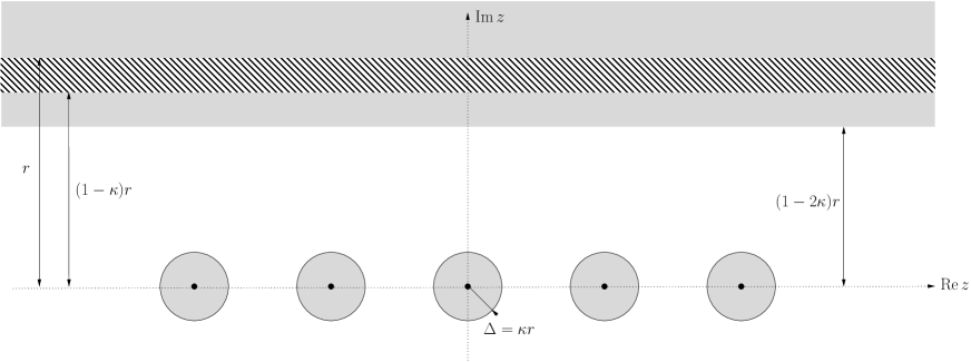
Figure 1: Picture of the $z$-plane (it is assumed here that $\kappa r<r_{\mathsf{S}}/4$). The black dots are the eigenvalues of $\mathcal{L}_{\mathsf{S}}$. If $\theta$ is in the hashed area, the spectrum of the deformed Liouvillean $\mathcal{L}_{\lambda,\alpha}(\theta)$ is in the shaded areas (which extends to infinity on the top side).

The first condition $\Delta\leq\kappa r$ ensures that the two subsets on the right-hand side of (4.5) are disjoint. It follows that the spectrum of $\mathcal{L}_{\lambda,\alpha}(\theta)$ in the subset $\{z\in\mathbb{C}\mid\mathop{\mathrm{dist}}(z,\mathop{\mathrm{sp}}(\mathcal{L}_{\mathsf{S}}))<\Delta\}$ is discrete. The second condition $\Delta\leq r_{\mathsf{S}}/4$ ensures that for any distinct $e,e^{\prime}\in\mathop{\mathrm{sp}}(\mathcal{L}_{\mathsf{S}})$

$$\{z\in\mathbb{C}\mid|z-e|<\Delta\}\cap\{z\in\mathbb{C}\mid|z-e^{\prime}|<\Delta\}=\emptyset,$$

so that the spectral projection

$$\mathcal{Q}_{\lambda,\alpha,e}(\theta)=\oint\limits_{|z-e|=r_{\mathsf{S}}/2}(z-\mathcal{L}_{\lambda,\alpha}(\theta))^{-1}\frac{\mathrm{d}z}{2\pi\mathrm{i}}$$

onto the part of spectrum of $\mathcal{L}_{\lambda,\alpha}(\theta)$ inside the disk $|z-e|<r_{\mathsf{S}}/2$ has exactly the same rank as the spectral projection $\mathbb{1}_{e}(\mathcal{L}_{\mathsf{S}})$ of $\mathcal{L}_{\mathsf{S}}$ for the eigenvalue $e$. This spectrum actually coincides with the spectrum of a linear map

$$\Sigma_{e}(\lambda,\alpha):\mathop{\mathrm{Ran}}\mathbb{1}_{e}(\mathcal{L}_{\mathsf{S}})\to\mathop{\mathrm{Ran}}\mathbb{1}_{e}(\mathcal{L}_{\mathsf{S}}),$$ (4.7)

called quasi-energy operator in [JP02], that does not depend on $\theta$. Hence, the spectrum of $\mathcal{L}_{\lambda,\alpha}(\theta)$ in the half-plane $\mathop{\mathrm{Im}}z<(1-2\kappa)r$ is discrete and independent of $\theta$ as long as $(1-\kappa)r<\mathop{\mathrm{Im}}\theta\leq r$. The finitely many eigenvalues in this half-plane are called spectral resonances of $\mathcal{L}_{\lambda,\alpha}$. We shall briefly recall the construction of the quasi-energy operators $\Sigma_{e}(\lambda,\alpha)$ in Section 4.2.1.

(f)

We start with the observation that, for $\mathop{\mathrm{Im}}\theta\geq 0$, $\left(\mathrm{e}^{\mathrm{i}t\mathcal{L}_{\mathrm{fr}}(\theta)}\right)_{t\geq 0}$ is a strongly continuous contraction semi-group on $\mathcal{H}$. It then follows that for all $(\lambda,\alpha)\in\mathbb{C}^{2}$ and $0\leq\mathop{\mathrm{Im}}\theta<\hat{r}$, $\left(\mathrm{e}^{\mathrm{i}t\mathcal{L}_{\lambda,\alpha}(\theta)}\right)_{t\geq 0}$ is also a strongly continuous semi-group on $\mathcal{H}$. For $t,\lambda,\theta\in\mathbb{R}$ and $\alpha\in\mathrm{i}\mathbb{R}$, one has

$$\mathrm{e}^{\mathrm{i}t\mathcal{L}_{\lambda,\alpha}(\theta)}=\mathfrak{G}_{\lambda,\alpha,\theta}^{t}\mathrm{e}^{\mathrm{i}t\mathcal{L}_{\mathrm{fr}}(\theta)}$$

with the unitary cocycle

$$\mathfrak{G}_{\lambda,\alpha,\theta}^{t}=\mathbb{1}+\sum_{n\geq 1}(\mathrm{i}\lambda t)^{n}\int\limits_{0\leq s_{1}\leq\cdots\leq s_{n}\leq 1}W_{ts_{1}}(\alpha,\theta)\cdots W_{ts_{n}}(\alpha,\theta)\mathrm{d}s_{1}\cdots\mathrm{d}s_{n},$$

where

$$W_{t}(\alpha,\theta)=\mathrm{e}^{\mathrm{i}t\mathcal{L}_{\mathrm{fr}}(\theta)}W(\alpha,\theta)\mathrm{e}^{-\mathrm{i}t\mathcal{L}_{\mathrm{fr}}(\theta)}.$$

By Assumptions (SFM5)–(SFM6), the map $(\alpha,\theta)\mapsto W_{t}(\alpha,\theta)\in\mathcal{B}(\mathcal{H})$ extends to an analytic function on $\mathbb{C}\times\mathfrak{I}(\hat{r})$, bounded for $(\alpha,\mathop{\mathrm{Im}}\theta)$ in any compact subset of $\mathbb{C}\times\,]-\hat{r},\hat{r}[$. It follows that for $t\in\mathbb{R}$, $(\lambda,\alpha,\theta)\mapsto\mathfrak{G}_{\lambda,\alpha,\theta}^{t}$ is an analytic function on $\mathbb{C}^{2}\times\mathfrak{I}(\hat{r})$, bounded for $(\lambda,\alpha,\mathop{\mathrm{Im}}\theta)$ in any compact subset of $\mathbb{C}^{2}\times\,]-\hat{r},\hat{r}[$. Note that since $U(\theta^{\prime})W_{t}(\alpha,\theta)U(-\theta^{\prime})=W_{t}(\alpha,\theta+\theta^{\prime})$ for $\theta^{\prime}\in\mathbb{R}$, one has

$$U(\theta^{\prime})\mathfrak{G}^{t}_{\lambda,\alpha,\theta}\Psi=\mathfrak{G}^{t}_{\lambda,\alpha,\theta+\theta^{\prime}}U(\theta^{\prime})\Psi.$$

Thus, if $\Psi$ is analytic for the group $(U(\theta))_{\theta\in\mathbb{R}}$ in a strip $0\leq\mathop{\mathrm{Im}}\theta<\rho\leq\hat{r}$, so is $\mathfrak{G}^{t}_{\lambda,\alpha,\theta}\Psi$, and the latter identity extends by analyticity.

The family $\left(\mathrm{e}^{\mathrm{i}\theta N}\right)_{\mathop{\mathrm{Im}}\theta\geq 0}$ is a strongly continuous contraction semi-group which is analytic in the open upper half-plane $\mathop{\mathrm{Im}}\theta>0$. Thus, if $\Psi\in\mathcal{H}$ is analytic for the group $(U(\theta))_{\theta\in\mathbb{R}}$ in a strip $0\leq\mathop{\mathrm{Im}}\theta<\rho$, then, for $t>0$, the map

$$\mathbb{R}\ni\theta\mapsto\mathrm{e}^{\mathrm{i}t\mathcal{L}_{\mathrm{fr}}(\theta)}U(\theta)\Psi=\mathrm{e}^{\mathrm{i}t\theta N}\mathrm{e}^{\mathrm{i}t\mathcal{L}_{\mathrm{fr}}}U(\theta)\Psi$$

has a bounded continuous extension to the strip $0\leq\mathop{\mathrm{Im}}\theta<\rho$ which is analytic in its interior. It follows that the same holds for the map

$$\mathbb{R}\ni\theta\mapsto U(\theta)\mathrm{e}^{\mathrm{i}t\mathcal{L}_{\mathrm{fr}}}\Psi,$$

and hence that the respective extensions satisfy

$$\mathrm{e}^{\mathrm{i}t\mathcal{L}_{\mathrm{fr}}(\theta)}U(\theta)\Psi=U(\theta)\mathrm{e}^{\mathrm{i}t\mathcal{L}_{\mathrm{fr}}}\Psi$$

for $0\leq\mathop{\mathrm{Im}}\theta<\rho$. Combined with the previous results, we conclude that

$$\mathfrak{G}_{\lambda,\alpha,\theta}^{t}\mathrm{e}^{\mathrm{i}t\mathcal{L}_{\mathrm{fr}}(\theta)}U(\theta)\Psi=\mathfrak{G}_{\lambda,\alpha,\theta}^{t}U(\theta)\mathrm{e}^{\mathrm{i}t\mathcal{L}_{\mathrm{fr}}}\Psi=U(\theta)\mathfrak{G}_{\lambda,\alpha,0}^{t}\mathrm{e}^{\mathrm{i}t\mathcal{L}_{\mathrm{fr}}}\Psi,$$

and so

$$\mathrm{e}^{\mathrm{i}t\mathcal{L}_{\lambda,\alpha}(\theta)}U(\theta)\Psi=U(\theta)\mathrm{e}^{\mathrm{i}t\mathcal{L}_{\lambda,\alpha}}\Psi.$$ (4.8)

For later use, see in particular Section 5.3, we summarize the above discussion in the following lemma.

Lemma 4.1.

If  $\Psi$ is analytic for the group $(U(\theta))_{\theta\in\mathbb{R}}$ in a strip $0\leq\mathop{\mathrm{Im}}\theta<\rho\leq\hat{r}$, then the map

$$\mathbb{R}\ni\theta\mapsto U(\theta)\mathrm{e}^{\mathrm{i}t\mathcal{L}_{\lambda,\alpha}}\Psi\in\mathcal{H}$$

has an analytic extension to the same strip, which is bounded and continuous on any closed substrip, and for any $\theta$ in this strip

$$\mathrm{e}^{\mathrm{i}t\mathcal{L}_{\lambda,\alpha}(\theta)}U(\theta)\Psi=U(\theta)\mathrm{e}^{\mathrm{i}t\mathcal{L}_{\lambda,\alpha}}\Psi.$$

4.2 The quasi-energy operators

In this section we first recall briefly the construction of the maps $\Sigma_{e}(\lambda,\alpha)$. They go back to [HP83] and we refer the reader to e.g. [HP83, JP96a, JP02] for more details. In a second part we study their connection with the Davies generator and the level-shift operator, see e.g. [Dav74, DJ03, DF06, JPW14]. This connection plays a key role in the study of spectral properties of $\Sigma(\lambda,\alpha)$, hence of $\mathcal{L}_{\lambda,\alpha}(\theta)$, and which is given in Section 4.2.3.

The standing assumptions in this section are the ones made in Paragraph (e) of the previous section.

4.2.1 Construction of $\Sigma_{e}(\lambda,\alpha)$

The map $(\lambda,\alpha)\mapsto\mathcal{Q}_{\lambda,\alpha,e}(\theta)$ is analytic and

$$\mathcal{Q}_{0,\alpha,e}(\theta)=\mathcal{Q}_{0,0,e}(\theta)=\mathbb{1}_{e}(\mathcal{L}_{\mathrm{fr}})=\mathbb{1}_{e}(\mathcal{L}_{\mathsf{S}})\otimes|\Omega_{\mathsf{R}}\rangle\langle\Omega_{\mathsf{R}}|.$$

It follows from the estimate (4.6) and the resolvent identity that, by possibly making $\Lambda$ smaller,

$$\sup_{\genfrac{}{}{0.0pt}{1}{|\lambda|<\Lambda}{\alpha\in B(\vartheta,\zeta)}}\|\mathcal{Q}_{\lambda,\alpha,e}(\theta)-\mathcal{Q}_{0,0,e}(\theta)\|<1$$

for all $e\in\mathop{\mathrm{sp}}(\mathcal{L}_{\mathsf{S}})$. This gives that the map

$$S_{\lambda,\alpha,e}(\theta)=\mathcal{Q}_{0,0,e}(\theta)\mathcal{Q}_{\lambda,\alpha,e}(\theta):\mathop{\mathrm{Ran}}\mathcal{Q}_{\lambda,\alpha,e}(\theta)\to\mathop{\mathrm{Ran}}\mathcal{Q}_{0,0,e}(\theta)$$

is an isomorphism, reducing to the identity for $\lambda=0$. The quasi-energy operator (4.7) is defined by

$$\Sigma_{e}(\lambda,\alpha)=S_{\lambda,\alpha,e}(\theta)\mathcal{Q}_{\lambda,\alpha,e}(\theta)\mathcal{L}_{\lambda,\alpha}(\theta)\mathcal{Q}_{\lambda,\alpha,e}(\theta)S_{\lambda,\alpha,e}(\theta)^{-1}.$$ (4.9)

As the notation suggests, $\Sigma_{e}(\lambda,\alpha)$ does not depend on $\theta$, see e.g. [JP96a]. In the following, it will be convenient to identify $\mathop{\mathrm{Ran}}S_{\lambda,\alpha,e}(\theta)=\mathop{\mathrm{Ran}}\mathbb{1}_{e}(\mathcal{L}_{\mathrm{fr}})=\mathop{\mathrm{Ran}}\mathbb{1}_{e}(\mathcal{L}_{\mathsf{S}})\otimes\Omega_{\mathsf{R}}$ with $\mathop{\mathrm{Ran}}\mathbb{1}_{e}(\mathcal{L}_{\mathsf{S}})$, so that $\Sigma_{e}(\lambda,\alpha)$ will act on the eigenspace of $\mathcal{L}_{\mathsf{S}}$ for its eigenvalue $e$.

By construction these quasi-energy operators satisfy

$$\mathop{\mathrm{sp}}\big{(}\Sigma_{e}(\lambda,\alpha)\big{)}=\mathop{\mathrm{sp}}\left(\mathcal{L}_{\lambda,\alpha}(\theta)\right)\cap\big{\{}z\in\mathbb{C}\,\big{|}\,|z-e|<r_{\mathsf{S}}/2\big{\}},$$

and have the following properties which follow from regular perturbation theory [Kat66, RS78, HP83].

1. The map $(\lambda,\alpha)\mapsto\Sigma_{e}(\lambda,\alpha)$ is analytic and

   $$\Sigma_{e}(\lambda,\alpha)=e\mathbb{1}_{e}(\mathcal{L}_{\mathsf{S}})+\lambda^{2}\Sigma_{e}^{(2)}(\alpha)+O(\lambda^{3}),$$ (4.10)

   where the estimate $O(\lambda^{3})$ is uniform in $\alpha\in B(\vartheta,\zeta)$. The term linear in $\lambda$ vanishes due to Assumption (SFM0), and it is at this point that (SFM0) enters critically in the proof.

2. A Fermi golden rule computation gives

   $$\Sigma_{e}^{(2)}(\alpha)=\lim_{\epsilon\uparrow 0}\mathbb{1}_{e}(\mathcal{L}_{\mathsf{S}})T_{\mathsf{S}}^{\ast}W(\alpha)(e+\mathrm{i}\epsilon-\mathcal{L}_{\mathrm{fr}})^{-1}W(\alpha)T_{\mathsf{S}}\mathbb{1}_{e}(\mathcal{L}_{\mathsf{S}}),$$ (4.11)

   where $T_{\mathsf{S}}:\mathcal{H}_{\mathsf{S}}\ni X\mapsto X\otimes\Omega_{\mathsf{R}}$ has the adjoint $T_{\mathsf{S}}^{\ast}X\otimes\Psi_{\mathsf{R}}=\langle\Omega_{\mathsf{R}},\Psi_{\mathsf{R}}\rangle X$.

3. $$\Sigma(\lambda,\alpha)=\bigoplus_{e\in\mathop{\mathrm{sp}}(\mathcal{L}_{\mathsf{S}})}\Sigma_{e}(\lambda,\alpha),\qquad\Sigma^{(2)}(\alpha)=\bigoplus_{e\in\mathop{\mathrm{sp}}(\mathcal{L}_{\mathsf{S}})}\Sigma_{e}^{(2)}(\alpha),$$

   defines two operators acting on $\mathcal{H}_{\mathsf{S}}$. The operator $\Sigma^{(2)}(\alpha)$ is the so-called level-shift operator for the triple $(\mathcal{H}_{\mathsf{S}},\mathcal{L}_{\mathrm{fr}},W(\alpha))$, see e.g. [DF06]. Equation (4.11) also allows to define $\Sigma_{e}^{(2)}(\alpha)$, hence $\Sigma^{(2)}(\alpha)$, for all $\alpha\in\mathbb{C}$.

4.2.2 Quasi-energy operators and deformed Davies generators

In this section we turn to the close relation between $\Sigma^{(2)}(\alpha)$ and the deformed Davies generator introduced in [JPW14]. We will use this connection in the next section to study spectral properties of $\Sigma^{(2)}(\alpha)$. Those of $\Sigma(\lambda,\alpha)$ will then follow from regular perturbation theory.

It follows from (SFM5) and (2.12) that

$$\mathcal{C}_{j,k,m}(t) =\omega_{j}\left(\varphi_{j}(f_{j,k,m})\varphi_{j}(\mathrm{e}^{\mathrm{i}th_{j}}f_{j,k,m})\right)$$

$$=\tfrac{1}{2}\langle f_{j,k,m},(\mathrm{e}^{\mathrm{i}th_{j}}(1-T_{j})+\mathrm{e}^{-\mathrm{i}th_{j}}T_{j})f_{j,k,m}\rangle$$

$$=\tfrac{1}{4}\int_{\mathbb{R}}\frac{\cosh\left((\beta_{j}/2+\mathrm{i}t)s\right)}{\cosh\left(\beta_{j}s/2\right)}\tilde{f}_{j,k,m}(-s)\tilde{f}_{j,k,m}(s)\mathrm{d}s$$

$$=\tfrac{1}{2}\int_{\mathbb{R}}\frac{\tilde{f}_{j,k,m}(-s)\tilde{f}_{j,k,m}(s)}{1+\mathrm{e}^{-\beta_{j}s}}\mathrm{e}^{\mathrm{i}ts}\mathrm{d}s,$$

and (SFM6) allows to deform the integration contour from $\mathbb{R}$ to $\mathbb{R}\pm\mathrm{i}a$, as long as $|a|<\pi/\beta_{j}$,

$$\mathcal{C}_{j,k,m}(t)=\tfrac{1}{2}\int_{\mathbb{R}}\frac{\tilde{f}_{j,k,m}(-(s\pm\mathrm{i}a))\tilde{f}_{j,k,m}(s\pm\mathrm{i}a)}{1+\mathrm{e}^{-\beta_{j}(s\pm\mathrm{i}a)}}\mathrm{e}^{\mathrm{i}t(s\pm\mathrm{i}a)}\mathrm{d}s.$$

This gives that $\mathcal{C}_{j,k,m}(t)=O(\mathrm{e}^{-a|t|})$ for all $j,k,m$, provided $0\leq a<\hat{r}$. Hence, it holds that

(SFM00) For some $\epsilon>0$ and all $j,k,m$,

$$\int_{0}^{\infty}|\mathcal{C}_{j,k,m}(t)|t^{\epsilon}\mathrm{d}t<\infty.$$

Denote by $\tau_{j,\lambda}$ the $C^{\ast}$-dynamics on $\mathcal{O}_{\mathsf{S}}\otimes\mathcal{O}_{j}$ generated by $\delta_{\mathsf{S}}+\delta_{j}+\mathrm{i}\lambda[V_{j},\,\cdot\;]$. Assumption (SFM0) and (SFM00) go back to [Dav74], where it was shown that, for all $X,Y\in\mathcal{O}_{\mathsf{S}}$,

$$\lim_{\genfrac{}{}{0.0pt}{1}{\lambda\to 0}{\lambda^{2}t=\xi}}\omega_{\mathsf{S}}\otimes\omega_{j}\left(X\tau_{0,j}^{-t}\circ\tau_{\lambda,j}^{t}(Y)\right)=\omega_{\mathsf{S}}\left(X\mathrm{e}^{\xi K_{j}}(Y)\right),$$ (4.12)

for some $K_{j}\in\mathcal{B}(\mathcal{O}_{\mathsf{S}})$. By similar arguments, see [DF06], one can show that

$$\lim_{\genfrac{}{}{0.0pt}{1}{\lambda\to 0}{\lambda^{2}t=\xi}}\omega\left(X\tau_{0}^{-t}\circ\tau_{\lambda}^{t}(Y)\right)=\omega_{\mathsf{S}}\left(X\mathrm{e}^{\xi K}(Y)\right),$$

with

$$K=\sum_{j}K_{j}.$$

$K_{j}$ is the Davies generator of the system $\mathsf{S}+\mathsf{R}_{j}$ and $K$ that of the full system $\mathsf{S}+\mathsf{R}$. The semi-groups $\left(\mathrm{e}^{tK_{j}}\right)_{t\geq 0}$ and $\left(\mathrm{e}^{tK}\right)_{t\geq 0}$ are completely positive and unital on $\mathcal{O}_{\mathsf{S}}$. If Assumption (SFM7) holds, these semi-groups are also positivity improving, see e.g. [Spo77, JPW14].

For $\alpha\in\mathbb{C}$, following [JPW14], we define the deformed Davies generators $K_{\alpha,j}$ and $K_{\alpha}$ acting on $\mathcal{O}_{\mathsf{S}}$ by

$$K_{\alpha,j}(X)=K_{j}\left(X\mathrm{e}^{\alpha\beta_{j}H_{\mathsf{S}}}\right)\mathrm{e}^{-\alpha\beta_{j}H_{\mathsf{S}}},\qquad K_{\alpha}=\sum_{j}K_{\alpha,j}.$$ (4.13)

We note that $K_{j}$ commutes with $\delta_{\mathsf{S}}$ (see [Dav74, Theorem 2.1] or [DF06, Theorem 6.1]) so that

$$K_{\alpha+z,j}(X)=\mathrm{e}^{-z\beta_{j}H_{\mathsf{S}}}K_{\alpha,j}\left(\mathrm{e}^{z\beta_{j}H_{\mathsf{S}}}X\right),$$ (4.14)

for all $z\in\mathbb{C}$. For $\alpha\in\mathbb{R}$, the semi-groups $\left(\mathrm{e}^{tK_{\alpha,j}}\right)_{t\geq 0}$ and $\left(\mathrm{e}^{tK_{\alpha}}\right)_{t\geq 0}$ are also completely positive, and they are moreover positivity improving if Assumption (SFM7) holds, see [JPW14, Theorem 3.1].

The following proposition gives the announced connection between these deformed Davies generators and the level-shift operators.

Proposition 4.2.

Suppose that (SFM0), (SFM5) and (SFM6) hold. Then, for all $\alpha\in\mathbb{R}$,

$$\Sigma^{(2)}(\alpha)=-\mathrm{i}K_{1/2-\alpha}.$$ (4.15)

Corollary 4.3.

Suppose that (SFM0), (SFM5) and (SFM6) hold. Then, for all $\alpha\in\mathbb{R}$ the semi-group $\left(\mathrm{e}^{\mathrm{i}t\Sigma^{(2)}(\alpha)}\right)_{t\geq 0}$ is completely positive, and unital when $\alpha=\frac{1}{2}$. If Assumption (SFM7) holds, then this semi-group is also positivity improving.

The relation (4.15) can be proven by direct computation, see e.g. [DJ03, Section 6.7] or [DF06]. Alternatively, one can give a structural proof following [DJ04] where (4.15) was established in the cases $\alpha=0$ and $\alpha=1/2$. For the reader’s convenience we finish this section with a proof of Proposition 4.2 along these lines.

Remark 4.4.

Proposition 4.2 can actually be proven under much more general condition than (SFM6). However, making this assumption does not affect the generality of our main result while allowing for a relatively simple proof of Lemma 4.5 below which is the main technical ingredient of the argument.

Recall that $\Omega_{j}$ is the vector representative of the state $\omega_{j}$ in the GNS Hilbert space of the $j^{\mathrm{th}}$ reservoir. Setting

$$\mathcal{L}_{\lambda,\alpha,j}=\mathcal{L}_{\mathsf{S}}+\mathcal{L}_{j}+\lambda W_{j}(\alpha),$$

one has the following lemma, compare with (4.12).

Lemma 4.5.

For all $X,Y\in\mathcal{B}(\mathcal{K}_{\mathsf{S}})$ and $\alpha\in\mathrm{i}\mathbb{R}$,

$$\lim_{\genfrac{}{}{0.0pt}{1}{\lambda\to 0}{\lambda^{2}t=\xi}}\langle X\otimes\Omega_{j},\mathrm{e}^{-\mathrm{i}t\mathcal{L}_{\mathsf{S}}}\mathrm{e}^{\mathrm{i}t\mathcal{L}_{\lambda,\alpha,j}}Y\otimes\Omega_{j}\rangle=\mathop{\mathrm{tr}}\nolimits(X^{\ast}\mathrm{e}^{\mathrm{i}\xi\Sigma^{(2)}_{j}(\alpha)}Y),$$

where $\Sigma_{j}^{(2)}(\alpha)$ is the level-shift operator for $(\mathcal{H}_{\mathsf{S}},\mathcal{L}_{\mathsf{S}}+\mathcal{L}_{j},W_{j}(\alpha))$,

$$\Sigma_{j}^{(2)}(\alpha)=\bigoplus_{e\in\mathop{\mathrm{sp}}(\mathcal{L}_{\mathsf{S}})}\lim_{\epsilon\uparrow 0}\mathbb{1}_{e}(\mathcal{L}_{\mathsf{S}})T_{\mathsf{S}}^{\ast}W_{j}(\alpha)(e+\mathrm{i}\epsilon-(\mathcal{L}_{\mathsf{S}}+\mathcal{L}_{j}))^{-1}W_{j}(\alpha)T_{\mathsf{S}}\mathbb{1}_{e}(\mathcal{L}_{\mathsf{S}}).$$ (4.16)

Proof.

The proof is an application of [DF06, Theorem 3.4]. In that theorem the only assumption which requires a comment is the following one: for some $\lambda_{0}>0$

$$\int_{0}^{\infty}\sup_{|\lambda|\leq\lambda_{0}}\left\|\mathcal{P}W_{j}(\alpha)\mathrm{e}^{\mathrm{i}t(1-\mathcal{P})\mathcal{L}_{\lambda,\alpha,j}(1-\mathcal{P})}W_{j}(\alpha)\mathcal{P}\right\|\,\mathrm{d}t<\infty,$$

where $\mathcal{P}=I_{\mathsf{S}}\otimes|\Omega_{j}\rangle\langle\Omega_{j}|$. To check it, we introduce complex deformations as in Section 4.1,

$$\mathcal{L}_{\lambda,\alpha,j}(\theta) =U(\theta)\mathcal{L}_{\lambda,\alpha,j}U(-\theta)=\mathcal{L}_{0,j}(\theta)+\lambda W_{j}(\alpha,\theta),$$

$$\mathcal{L}_{0,j}(\theta) =\mathcal{L}_{\mathsf{S}}+\mathcal{L}_{j}+\theta N_{j}.$$

For $\mathop{\mathrm{Im}}\theta\geq 0$, $\left(\mathrm{e}^{\mathrm{i}t\mathcal{L}_{0,j}(\theta)}\right)_{t\geq 0}$ is a strongly continuous contraction semi-group on $\mathcal{H}_{\mathsf{S}}\otimes\mathcal{H}_{j}$. Hence, for all $\lambda,\alpha\in\mathbb{C}$ and $0\leq\mathop{\mathrm{Im}}\theta<\hat{r}$, the perturbed family $\left(\mathrm{e}^{\mathrm{i}t\mathcal{L}_{\lambda,\alpha,j}(\theta)}\right)_{t\geq 0}$ is a strongly continuous semi-group on $\mathcal{H}_{\mathsf{S}}\otimes\mathcal{H}_{j}$. Moreover, since $\mathcal{P}U(\theta)=\mathcal{P}=U(-\theta)\mathcal{P}$, we can write

$$\mathcal{P}W_{j}(\alpha)\mathrm{e}^{\mathrm{i}t(1-\mathcal{P})\mathcal{L}_{\lambda,\alpha,j}(1-\mathcal{P})}W_{j}(\alpha)\mathcal{P}=\mathcal{P}W_{j}(\alpha,\theta)\mathrm{e}^{\mathrm{i}t(1-\mathcal{P})\mathcal{L}_{\lambda,\alpha,j}(\theta)(1-\mathcal{P})}W_{j}(\alpha,\theta)\mathcal{P}.$$ (4.17)

It follows from (SFM0) that $\mathcal{P}V_{j}\mathcal{P}=0$, and similarly $\mathcal{P}W(\alpha,\theta)\mathcal{P}=0$. It therefore suffices to prove that

$$\int_{0}^{\infty}\sup_{|\lambda|\leq\lambda_{0}}\left\|(1-\mathcal{P})\mathrm{e}^{\mathrm{i}t(1-\mathcal{P})\mathcal{L}_{\lambda,\alpha,j}(\theta)(1-\mathcal{P})}(1-\mathcal{P})\right\|\,\mathrm{d}t<\infty,$$ (4.18)

for some $\lambda_{0}>0$ and some $\theta$ such that $0\leq\mathop{\mathrm{Im}}\theta<\hat{r}$. Observing that the operator appearing in the last formula belongs to the semi-group acting on $\mathop{\mathrm{Ker}}\mathcal{P}$ and generated by

$$(1-\mathcal{P})\mathcal{L}_{\lambda,\alpha,j}(\theta)|_{\mathop{\mathrm{Ker}}\mathcal{P}}=\mathcal{L}_{\mathsf{S}}+\mathrm{d}\Gamma(s+\theta)|_{\Omega_{j}^{\perp}}+\lambda(1-\mathcal{P})W(\alpha,\theta)|_{\mathop{\mathrm{Ker}}\mathcal{P}},$$

we get, for $\lambda=0$ and $t\geq 0$,

$$\left\|(1-\mathcal{P})\mathrm{e}^{\mathrm{i}t(1-\mathcal{P})\mathcal{L}_{0,j}(\theta)(1-\mathcal{P})}(1-\mathcal{P})\right\|=\mathrm{e}^{-t\mathop{\mathrm{Im}}(\theta)},$$

and a standard estimate on perturbed semi-groups [Dav80, Theorem 3.1] gives

$$\|(1-\mathcal{P})\mathrm{e}^{\mathrm{i}t(1-\mathcal{P})\mathcal{L}_{\lambda,\alpha,j}(\theta)(1-\mathcal{P})}(1-\mathcal{P})\|\leq\mathrm{e}^{-t(\mathop{\mathrm{Im}}\theta-|\lambda|\|W(\alpha,\theta)\|)},$$

so that the estimate (4.18) follows by fixing $\theta$ such that $0<\mathop{\mathrm{Im}}(\theta)<\hat{r}$ and $0<\lambda_{0}$ small enough.

Proof of Proposition 4.2. For $\alpha\in\mathrm{i}\mathbb{R}$ we have that

$$V_{j}^{\#}(\alpha)=(J_{\mathsf{S}}\otimes J_{j})(\mathrm{e}^{\alpha\beta_{j}\mathcal{L}_{j}}V_{j}\mathrm{e}^{-\alpha\beta_{j}\mathcal{L}_{j}})(J_{\mathsf{S}}\otimes J_{j})=\mathrm{e}^{\alpha\beta_{j}\mathcal{L}_{j}}(J_{\mathsf{S}}\otimes J_{j})V_{j}(J_{\mathsf{S}}\otimes J_{j})\mathrm{e}^{-\alpha\beta_{j}\mathcal{L}_{j}}.$$

Consider now the operator $H_{\mathsf{S}}+\mathcal{L}_{j}+\lambda V_{j}$ where, with the usual abuse of notation, $H_{\mathsf{S}}$ stands for $\pi(H_{\mathsf{S}})$, and so $H_{\mathsf{S}}+\lambda V_{j}\in\pi(\mathcal{O})$. By the Trotter product formula,

$$\mathrm{e}^{\alpha\beta_{j}(H_{\mathsf{S}}+\mathcal{L}_{j}+\lambda V_{j})}(J_{\mathsf{S}}\otimes J_{j}) V_{j}(J_{\mathsf{S}}\otimes J_{j})\mathrm{e}^{-\alpha\beta_{j}(H_{\mathsf{S}}+\mathcal{L}_{j}+V_{j})}$$

$$=\lim_{n\to\infty}\left(\mathrm{e}^{\alpha\beta_{j}(H_{\mathsf{S}}+\lambda V_{j})/n}\mathrm{e}^{\alpha\beta_{j}\mathcal{L}_{j}/n}\right)^{n}(J_{\mathsf{S}}\otimes J_{j}) V_{j}(J_{\mathsf{S}}\otimes J_{j})\left(\mathrm{e}^{-\alpha\beta_{j}(H_{\mathsf{S}}+V_{j})/n}\mathrm{e}^{-\alpha\beta_{j}\mathcal{L}_{j}/n}\right)^{n}.$$

Since, for $t\in\mathbb{R}$, $\mathrm{e}^{\mathrm{i}t\mathcal{L}_{j}}\pi(\mathcal{O})^{\prime}\mathrm{e}^{-\mathrm{i}t\mathcal{L}_{j}}\subset\pi(\mathcal{O})^{\prime}$, we derive that for $\alpha\in\mathrm{i}\mathbb{R}$,

$$V_{j}^{\#}(\alpha)=\mathrm{e}^{\alpha\beta_{j}(H_{\mathsf{S}}+\mathcal{L}_{j}+\lambda V_{j})}(J_{\mathsf{S}}\otimes J_{j})V_{j}(J_{\mathsf{S}}\otimes J_{j})\mathrm{e}^{-\alpha\beta_{j}(H_{\mathsf{S}}+\mathcal{L}_{j}+\lambda V_{j})}.$$ (4.19)

Using that $\mathcal{L}_{\mathsf{S}}+\mathcal{L}_{j}+\lambda V_{j}=\mathcal{L}_{\lambda,\alpha,j}-\lambda V_{j}^{\#}(\alpha)$ commutes with $H_{\mathsf{S}}+\mathcal{L}_{j}+\lambda V_{j}$, (4.19) further yields that

$$\mathcal{L}_{\lambda,\alpha,j}=\mathrm{e}^{\alpha\beta_{j}(H_{\mathsf{S}}+\mathcal{L}_{j}+\lambda V_{j})}\mathcal{L}_{\lambda,0,j}\mathrm{e}^{-\alpha\beta_{j}(H_{\mathsf{S}}+\mathcal{L}_{j}+\lambda V_{j})}.$$

Combined with Lemma 4.5, this relation gives that, for $\alpha\in\mathrm{i}(-\zeta,\zeta)$,

$$\Sigma_{j}^{(2)}(\alpha)(X)=\mathrm{e}^{\alpha\beta_{j}H_{\mathsf{S}}}\Sigma_{j}^{(2)}(0)(\mathrm{e}^{-\alpha\beta_{j}H_{\mathsf{S}}}X).$$ (4.20)

By analyticity, this relation holds for all $\alpha\in\mathbb{R}$, provided its left-hand side is given by (4.16). It was shown in [DJ04, Theorem 3.1] that

$$\Sigma_{j}^{(2)}(0)=-\mathrm{i}K_{1/2,j},$$

and so

$$\Sigma^{(2)}(\alpha)(X)=\sum_{j}\Sigma_{j}^{(2)}(\alpha)(X)=\sum_{j}\mathrm{e}^{\alpha\beta_{j}H_{\mathsf{S}}}\Sigma_{j}^{(2)}(0)(\mathrm{e}^{-\alpha\beta_{j}H_{\mathsf{S}}}X)=-\mathrm{i}\sum_{j}\mathrm{e}^{\alpha\beta_{j}H_{\mathsf{S}}}K_{1/2,j}(\mathrm{e}^{-\alpha\beta_{j}H_{\mathsf{S}}}X).$$

Taking into account (4.13)–(4.14), we finally get

$$\Sigma^{(2)}(\alpha)=-\mathrm{i}\sum_{j}K_{1/2-\alpha,j}=-\mathrm{i}K_{1/2-\alpha}.$$

4.2.3 Spectral analysis of $\Sigma(\lambda,\alpha)$

As a direct consequence of Corollary 4.3 we first get the following spectral result about the level-shift operator $\Sigma^{(2)}(\alpha)$, see e.g. [JPW14, Theorem 2.2]. Let

$$\mathcal{E}^{(2)}(\alpha)=\mathrm{i}\,\min\left\{\mathop{\mathrm{Im}}w\mid w\in\mathop{\mathrm{sp}}\left(\Sigma^{(2)}(\alpha)\right)\right\}.$$

Lemma 4.6.

Assuming (SFM0) and (SFM5)–(SFM7), the following assertions hold for $\alpha\in\mathbb{R}$.

1. $\mathcal{E}^{(2)}(\alpha)$ is a purely imaginary simple eigenvalue of  $\Sigma^{(2)}(\alpha)$, with $\mathcal{E}^{(2)}\left(\tfrac{1}{2}\right)=0$.

2. All the other eigenvalues  $z\in\mathop{\mathrm{sp}}\left(\Sigma^{(2)}(\alpha)\right)\setminus\left\{\mathcal{E}^{(2)}(\alpha)\right\}$ satisfy  $\mathop{\mathrm{Im}}\left(z-\mathcal{E}^{(2)}(\alpha)\right)>0$.

3. The eigenprojection for the eigenvalue $\mathcal{E}^{(2)}(\alpha)$ writes $P_{\alpha}=|X_{\alpha}\rangle\langle Y_{\alpha}|$, where $X_{\alpha},Y_{\alpha}\in\mathcal{H}_{\mathsf{S}}=\mathcal{B}(\mathcal{K}_{\mathsf{S}})$ are positive definite.

Proposition 4.7.

Under the assumptions of the previous lemma, for any $\vartheta,\zeta>0$ there exists $\Lambda,\epsilon>0$ such that:

1. For $0<|\lambda|<\Lambda$ and $\alpha\in B(\vartheta,\zeta)$, the linear map $\Sigma(\lambda,\alpha)$ has a simple eigenvalue $\mathcal{E}(\lambda,\alpha)$ such that for any other eigenvalue $w\in\mathop{\mathrm{sp}}(\Sigma(\lambda,\alpha))\setminus\{\mathcal{E}(\lambda,\alpha)\}$ one has

   $$\mathop{\mathrm{Im}}(w-\mathcal{E}(\lambda,\alpha))\geq\lambda^{2}\epsilon.$$

2. For fixed $\lambda$, the map $B(\vartheta,\zeta)\ni\alpha\mapsto\mathcal{E}(\lambda,\alpha)$ is analytic.

3. $\mathcal{E}(\lambda,\alpha)\in\mathop{\mathrm{sp}}(\Sigma_{0}(\lambda,\alpha))$, in particular $|\mathcal{E}(\lambda,\alpha)|<\frac{r_{\mathsf{S}}}{4}$.

Proof.

(1)–(2) Follow immediately from (4.10), the previous lemma and regular perturbation theory.

(3) Since $\mathcal{E}^{(2)}(\alpha)$ is purely imaginary it must be an eigenvalue of $\Sigma_{0}^{(2)}(\alpha)$. Regular perturbation theory ensures that $\mathcal{E}(\lambda,\alpha)$ is therefore an eigenvalue of $\Sigma_{0}(\lambda,\alpha)$ for $\lambda$ small enough.

Remark 4.8.

Using (4.10) we actually have $\mathcal{E}(\lambda,\alpha)=\lambda^{2}\mathcal{E}^{(2)}(\alpha)+O(\lambda^{3})$.

4.3 Dynamics of $\alpha$-Liouvilleans

In this and the next two sections, we assume that (SFM0) and (SFM5)–(SFM7) hold, and we set

$$D=\bigcap_{|\mathop{\mathrm{Im}}\theta|<\hat{r}}\mathop{\mathrm{Dom}}U(\theta).$$

Recall also that $0<r<\hat{r}$ is fixed and $C$ is given by (4.4).

Proposition 4.9.

For any $\tfrac{2}{3}r<\varrho<r$ and $\vartheta,\zeta>0$, there exist constants $\Lambda,\epsilon>0$ such that, for $\alpha\in B(\vartheta,\zeta)$, $0<|\lambda|<\Lambda$, and $\Phi,\Psi\in D$, the function

$$z\mapsto\langle\Phi,(z-\mathcal{L}_{\lambda,\alpha})^{-1}\Psi\rangle,$$ (4.21)

originally analytic for $\mathop{\mathrm{Im}}z<-\Lambda C$, has a meromorphic continuation to the half-plane $\mathop{\mathrm{Im}}z<\varrho$, and its only possible singularity in the region $\mathop{\mathrm{Im}}(z-\mathcal{E}(\lambda,\alpha))<\tfrac{1}{2}\lambda^{2}\epsilon$ is a simple pole at $\mathcal{E}(\lambda,\alpha)$.

Proof.

Fix $0<\kappa<\frac{1}{6}$ such that $\varrho=(1-2\kappa)r$. Let $\Lambda,\epsilon$ be as Proposition 4.7 and $\Phi,\Psi\in D$. For all $\mathop{\mathrm{Im}}z<-\Lambda C$ and $\theta\in\mathbb{R}$ one has

$$\langle\Phi,(z-\mathcal{L}_{\lambda,\alpha})^{-1}\Psi\rangle=\langle U(\theta)\Phi,(z-\mathcal{L}_{\lambda,\alpha}(\theta))^{-1}U(\theta)\Psi\rangle.$$

Note that the functions $\mathbb{R}\ni\theta\mapsto\Psi_{\theta}=U(\theta)\Psi$ and $\mathbb{R}\ni\theta\mapsto\overline{\Phi}_{\theta}=\overline{U(\theta)\Phi}=U(-\theta)\overline{\Phi}$ both have analytic continuations to the strip $\mathfrak{I}(\hat{r})$. Thus, the identity

$$\langle\Phi,(z-\mathcal{L}_{\lambda,\alpha})^{-1}\Psi\rangle=\left\langle\overline{\overline{\Phi}_{\theta}},(z-\mathcal{L}_{\lambda,\alpha}(\theta))^{-1}\Psi_{\theta}\right\rangle$$ (4.22)

holds for all $\theta\in\mathfrak{I}^{+}(\hat{r})$, $|\lambda|<\Lambda$, $\alpha\in B(\vartheta,\zeta)$ and $\mathop{\mathrm{Im}}z<-\Lambda C$. Using the results from Paragraph (e) in Section 4.1, by setting $\theta=\mathrm{i}r$ the right-hand side of this identity provides a meromorphic continuation of its left-hand side to the half-plane $\mathop{\mathrm{Im}}z<\varrho$. Proposition 4.7 then yields the last assertion.

Remark 4.10.

The residue of the function (4.21) at $\mathcal{E}(\lambda,\alpha)$ is given by

$$c_{\lambda,\alpha}=\langle U(-\mathrm{i}r)\Phi,\mathcal{Q}_{\lambda,\alpha}(\mathrm{i}r)U(\mathrm{i}r)\Psi\rangle,$$ (4.23)

where $\mathcal{Q}_{\lambda,\alpha}(\mathrm{i}r)$ is the spectral projection of $\mathcal{L}_{\lambda,\alpha}(\mathrm{i}r)$ for the eigenvalue $\mathcal{E}(\lambda,\alpha)$.

Proposition 4.11.

For any $\tfrac{2}{3}r<\varrho<r$ and $\vartheta,\zeta>0$, there exist a constants $\Lambda>0$ such that, for $\alpha\in B(\vartheta,\zeta)$, $0<|\lambda|<\Lambda$, and $\phi,\psi\in\mathcal{H}$, the function $f(z)=\langle\phi,(z-\mathcal{L}_{\lambda,\alpha}(\mathrm{i}r))^{-1}\psi\rangle$ satisfies

$$\sup_{\genfrac{}{}{0.0pt}{1}{y<\varrho}{j\in\{0,1\}}}\int_{|x|>R}|(\partial^{j}f)(x+\mathrm{i}y)|^{2-j}\,\mathrm{d}x<+\infty,$$ (4.24)

where $R=1+\|\mathcal{L}_{\mathsf{S}}\|$. As a consequence, for any $\Phi,\Psi\in D$, the function $g(z)=\langle\Phi,(z-\mathcal{L}_{\lambda,\alpha})^{-1}\Psi\rangle$ satisfies

$$\sup_{\genfrac{}{}{0.0pt}{1}{y<\varrho}{j\in\{0,1\}}}\int_{|x|>R}|(\partial^{j}g)(x+\mathrm{i}y)|^{2-j}\,\mathrm{d}x<+\infty.$$ (4.25)

Proof.

As in the proof of Proposition 4.9, we fix $0<\kappa<1/6$ such that $\varrho=(1-2\kappa)r$.

Since $\mathcal{L}_{\mathrm{fr}}(\mathrm{i}r)$ is a normal operator, the spectral theorem gives that for $z$ in the resolvent set of $\mathcal{L}_{\mathrm{fr}}(\mathrm{i}r)$,

$$\|(z-\mathcal{L}_{\mathrm{fr}}(\mathrm{i}r))^{-1}\psi\|^{2}=\int_{\mathop{\mathrm{sp}}(\mathcal{L}_{\mathrm{fr}}(\mathrm{i}r))}\frac{\mathrm{d}\mu_{\psi}(\xi)}{|z-\xi|^{2}},$$

where $\mu_{\psi}$ denotes the spectral measure of $\mathcal{L}_{\mathrm{fr}}(\mathrm{i}r)$ for the vector $\psi$.

For any $\xi\in\mathop{\mathrm{sp}}(\mathcal{L}_{\mathrm{fr}}(\mathrm{i}r))$ and $y<\varrho$, one has

$$\int_{|x|>R}\frac{\mathrm{d}x}{|x+\mathrm{i}y-\xi|^{2}}\leq\max\left(\frac{\pi}{2\kappa r},2\right),$$

and hence

$$\sup_{y<\varrho}\int_{|x|>R}\|(x+\mathrm{i}y-\mathcal{L}_{\mathrm{fr}}(\mathrm{i}r))^{-1}\psi\|^{2}\mathrm{d}x<\infty.$$ (4.26)

By the same argument, we also have

$$\sup_{y<\varrho}\int_{|x|>R}\|\left((x+\mathrm{i}y-\mathcal{L}_{\mathrm{fr}}(\mathrm{i}r))^{-1}\right)^{\ast}\phi\|^{2}\mathrm{d}x<\infty.$$ (4.27)

Invoking the identity (4.3), we deduce that if $\Lambda$ is small enough then, for $|\lambda|<\Lambda$ and $\alpha\in B(\vartheta,\zeta)$, the operator

$$G(z,\lambda,\alpha)=\left(I-\lambda(z-\mathcal{L}_{\mathrm{fr}}(\mathrm{i}r))^{-1}W(\alpha,\mathrm{i}r)\right)^{-1}$$

is well defined for $|\mathop{\mathrm{Re}}z|>R$, $\mathop{\mathrm{Im}}z<\varrho$, and satisfies

$$\sup_{\genfrac{}{}{0.0pt}{1}{|\mathop{\mathrm{Re}}z|>R}{\mathop{\mathrm{Im}}z<\varrho}}\|G(z,\lambda,\alpha)\|\leq 2.$$ (4.28)

It follows from the second resolvent identity that

$$(z-\mathcal{L}_{\lambda,\alpha}(\mathrm{i}r))^{-1}=G(z,\lambda,\alpha)(z-\mathcal{L}_{\mathrm{fr}}(\mathrm{i}r))^{-1}.$$ (4.29)

Combining (4.26), (4.28) and (4.29) gives that (4.24) holds for $j=0$.

Similarly, the operator

$$\widetilde{G}(z,\lambda,\alpha)=\left(I-\lambda W(\alpha,\mathrm{i}r)(z-\mathcal{L}_{\mathrm{fr}}(\mathrm{i}r))^{-1}\right)^{-1}$$

also satisfies

$$\sup_{\genfrac{}{}{0.0pt}{1}{|\mathop{\mathrm{Re}}z|>R}{\mathop{\mathrm{Im}}z<\varrho}}\|\widetilde{G}(z,\lambda,\alpha)\|\leq 2,$$

and is such that

$$(z-\mathcal{L}_{\lambda,\alpha}(\mathrm{i}r))^{-1}=(z-\mathcal{L}_{\mathrm{fr}}(\mathrm{i}r))^{-1}\widetilde{G}(z,\lambda,\alpha).$$

We can then write

$$-\partial(z-\mathcal{L}_{\lambda,\alpha}(\mathrm{i}r))^{-1}=(z-\mathcal{L}_{\lambda,\alpha}(\mathrm{i}r))^{-2}=(z-\mathcal{L}_{\mathrm{fr}}(\mathrm{i}r))^{-1}\widetilde{G}(z,\lambda,\alpha)G(z,\lambda,\alpha)(z-\mathcal{L}_{\mathrm{fr}}(\mathrm{i}r))^{-1},$$

so that

$$|\partial f(z)|=\left|\partial\langle\phi,(z-\mathcal{L}_{\lambda,\alpha}(\mathrm{i}r))^{-1}\psi\rangle\right|\leq 4\|\left((z-\mathcal{L}_{\mathrm{fr}}(\mathrm{i}r))^{-1}\right)^{\ast}\phi\|\,\|(z-\mathcal{L}_{\mathrm{fr}}(\mathrm{i}r))^{-1}\psi\|.$$

Combining (4.26), (4.27) and the Cauchy-Schwarz inequality, we obtain (4.24) with $j=1$.

Finally, (4.25) follows from (4.22) and (4.24) with $\theta=\mathrm{i}r$, $\phi=U(-\mathrm{i}r)\Phi$ and $\psi=U(\mathrm{i}r)\Psi$.

Using Propositions 4.9 and 4.11 together with [BBJ⁺24a, Proposition 4.1] we obtain the following dynamical result.

Proposition 4.12.

For any $\vartheta,\zeta>0$ there exists $\Lambda,\epsilon>0$ such that for any $0<|\lambda|<\Lambda$, $\alpha\in B(\vartheta,\zeta)$ and $\Phi,\Psi\in D$ one has

$$\langle\Phi,\mathrm{e}^{\mathrm{i}t\mathcal{L}_{\lambda,\alpha}}\Psi\rangle=\mathrm{e}^{\mathrm{i}t\mathcal{E}(\lambda,\alpha)}\left(c_{\lambda,\alpha}+O(\mathrm{e}^{-\lambda^{2}\epsilon t})\right)$$

as $t\uparrow\infty$, where $c_{\lambda,\alpha}$ is the residue given by (4.23).

The next, closely related, result is proven in an identical way and will be used in the sequel. Recall that, for all $(\lambda,\alpha)\in\mathbb{C}^{2}$ and $0\leq\mathop{\mathrm{Im}}\theta<\hat{r}$, $\left(\mathrm{e}^{\mathrm{i}t\mathcal{L}_{\lambda,\alpha}(\theta)}\right)_{t\geq 0}$ is also a strongly continuous semi-group on $\mathcal{H}$. Combining (4.24) in Proposition 4.11 with the spectral results about $\mathcal{L}_{\lambda,\alpha}(\theta)$ obtained in Sections 4.1–4.2, and using [BBJ⁺24a, Proposition 4.1], we have the following analogue of Proposition 4.12.

Proposition 4.13.

For any $\vartheta,\zeta>0$, there exist constants $\Lambda,\epsilon>0$ such that, for all $0<|\lambda|<\Lambda$, $\alpha\in B(\vartheta,\zeta)$ and $\phi,\psi\in\mathcal{H}$ one has

$$\langle\phi,\mathrm{e}^{\mathrm{i}t\mathcal{L}_{\lambda,\alpha}(\mathrm{i}r)}\psi\rangle=\mathrm{e}^{\mathrm{i}t\mathcal{E}(\lambda,\alpha)}\left(\langle\phi,\mathcal{Q}_{\lambda,\alpha}(\mathrm{i}r)\psi\rangle+O(\mathrm{e}^{-\lambda^{2}\epsilon t})\right)$$

as $t\uparrow\infty$.

4.4 The $\widehat{\mathcal{L}}_{\lambda,\alpha}$ Liouvilleans

As mentioned in Section 3.3, the study of the ancilla part of the PREF relies on the closely related Liouvilleans $\widehat{\mathcal{L}}_{\lambda,\alpha}$. It is easy to see that the analysis of $\mathcal{L}_{\lambda,\alpha}$ presented in the previous sections extends line by line to $\widehat{\mathcal{L}}_{\lambda,\alpha}$ and the associated analytically deformed $\widehat{\mathcal{L}}_{\lambda,\alpha}(\theta)$. We denote by $\widehat{\Sigma}^{(2)}(\alpha)$ and $\widehat{\Sigma}(\lambda,\alpha)$ the corresponding level-shift and quasi-energy operators.

By the definition (3.6), $\widehat{\mathcal{L}}_{\lambda,\alpha}$ is obtained from $\mathcal{L}_{\lambda,\alpha}$ by replacing $W(\alpha)$ by $\Delta_{\omega}^{-\alpha/2}W\left(\tfrac{1}{2}-\alpha\right)\Delta_{\omega}^{\alpha/2}$. Since $\Delta_{\omega}^{\alpha/2}$ commutes with $\mathcal{L}_{\mathrm{fr}}$ and $\Delta_{\omega}^{\alpha/2}T_{\mathsf{S}}=T_{\mathsf{S}}$, the associated level-shift operator is given by

$$\widehat{\Sigma}_{e}^{(2)}(\alpha) =\lim_{\epsilon\uparrow 0}\mathbb{1}_{e}(\mathcal{L}_{\mathsf{S}})T_{\mathsf{S}}^{\ast}\Delta_{\omega}^{-\alpha/2}W\left(\tfrac{1}{2}-\alpha\right)\Delta_{\omega}^{\alpha/2}(e+\mathrm{i}\epsilon-\mathcal{L}_{\mathrm{fr}})^{-1}\Delta_{\omega}^{-\alpha/2}W\left(\tfrac{1}{2}-\alpha\right)\Delta_{\omega}^{\alpha/2}T_{\mathsf{S}}\mathbb{1}_{e}(\mathcal{L}_{\mathsf{S}})$$

$$=\lim_{\epsilon\uparrow 0}\mathbb{1}_{e}(\mathcal{L}_{\mathsf{S}})T_{\mathsf{S}}^{\ast}W\left(\tfrac{1}{2}-\alpha\right)(e+\mathrm{i}\epsilon-\mathcal{L}_{\mathrm{fr}})^{-1}W\left(\tfrac{1}{2}-\alpha\right)T_{\mathsf{S}}\mathbb{1}_{e}(\mathcal{L}_{\mathsf{S}})$$

$$=\Sigma_{e}^{(2)}\left(\tfrac{1}{2}-\alpha\right),$$

for $\alpha\in\mathrm{i}\mathbb{R}$, hence for all $\alpha\in\mathbb{C}$ by analyticity. In particular the conclusions of Corollary 4.3 hold, with unital property when $\alpha=0$, hence so do those of Lemma 4.6 and Proposition 4.7, i.e., the operator $\widehat{\Sigma}(\lambda,\alpha)$ has a simple eigenvalue $\widehat{\mathcal{E}}(\lambda,\alpha)$ such that for any other eigenvalue $w$ of $\widehat{\Sigma}(\lambda,\alpha)$ one has

$$\mathop{\mathrm{Im}}\left(w-\widehat{\mathcal{E}}(\lambda,\alpha)\right)\geq\lambda^{2}\epsilon.$$

Arguing as in Section 4.1, Paragraph (f), we derive that, for all $\lambda,\alpha\in\mathbb{C}$ and $0\leq\mathop{\mathrm{Im}}\theta<\hat{r}$, the family $\left(\mathrm{e}^{\mathrm{i}t\widehat{\mathcal{L}}_{\lambda,\alpha}(\theta)}\right)_{t\geq 0}$ is a strongly continuous semi-group on $\mathcal{H}$ such that, similarly with (4.8), one has

$$U(\theta)\mathrm{e}^{\mathrm{i}t\widehat{\mathcal{L}}_{\lambda,\alpha}}\Psi=\mathrm{e}^{\mathrm{i}t\widehat{\mathcal{L}}_{\lambda,\alpha}(\theta)}U(\theta)\Psi$$ (4.30)

for all $\Psi\in D$ and $0\leq\mathop{\mathrm{Im}}\theta<\hat{r}$. Finally, we have the following analogue of Propositions 4.12 and 4.13.

Proposition 4.14.

For any $\vartheta,\zeta>0$, there exists $\Lambda,\epsilon>0$ such that for all $0<|\lambda|<\Lambda$, $\alpha\in B(\vartheta,\zeta)$ and all $\Phi,\Psi\in D$ one has

$$\langle\Phi,\mathrm{e}^{\mathrm{i}t\widehat{\mathcal{L}}_{\lambda,\alpha}}\Psi\rangle=\mathrm{e}^{\mathrm{i}t\widehat{\mathcal{E}}(\lambda,\alpha)}\left(\langle U(-\mathrm{i}r)\Phi,\widehat{\mathcal{Q}}_{\lambda,\alpha}(\mathrm{i}r)U(\mathrm{i}r)\Psi\rangle+O(\mathrm{e}^{-\lambda^{2}\epsilon t})\right)$$ (4.31)

as $t\uparrow\infty$, and where $\widehat{\mathcal{Q}}_{\lambda,\alpha}(\mathrm{i}r)$ is the spectral projection of $\widehat{\mathcal{L}}_{\lambda,\alpha}(\mathrm{i}r)$ for its eigenvalue $\widehat{\mathcal{E}}(\lambda,\alpha)$.

Similarly, for all $\phi,\psi\in\mathcal{H}$ one has

$$\langle\phi,\mathrm{e}^{\mathrm{i}t\widehat{\mathcal{L}}_{\lambda,\alpha}(\mathrm{i}r)}\psi\rangle=\mathrm{e}^{\mathrm{i}t\widehat{\mathcal{E}}(\lambda,\alpha)}\left(\langle\phi,\widehat{\mathcal{Q}}_{\lambda,\alpha}(\mathrm{i}r)\psi\rangle+O(\mathrm{e}^{-\lambda^{2}\epsilon t})\right),$$ (4.32)

as $t\uparrow\infty$.

5 Proof of Theorem 2.8

We prove separately the 2TMEP, QPSC and EAST parts of the PREF. These three parts are proven respectively in Sections 5.2, 5.3 and 5.4. They all rely on the representation of the various entropic functionals given in Proposition 3.2 and on Propositions 4.12, 4.13 and 4.14.

As a preparation for the proof we establish some analyticity properties of the Connes cocycle. Indeed, for the QPSC and Ancilla parts of the PREF we will first have to consider the large $T$ limit in Proposition 3.2(2)–(3) in order to obtain suitable expressions for $\mathfrak{F}_{\omega_{+},t}^{\mathrm{ancilla}}$ and $\mathfrak{F}_{\omega_{+},t}^{\mathrm{qpsc}}$. This large $T$ limit also relies on Proposition 4.12, applied to $\mathrm{e}^{iT\mathcal{L}_{\lambda,1/2}}$. For that purpose one needs to prove that the vectors

$$[D\omega_{-t}:D\omega]_{\alpha}\Omega\qquad\text{and}\qquad[D\omega_{-t}:D\omega]^{\ast}_{\frac{\bar{\alpha}}{2}}[D\omega_{-t}:D\omega]_{\frac{\alpha}{2}}\Omega$$

belong to the subspace $D$. This will be a consequence of the analyticity properties of the Connes cocycle we establish in the next section.

5.1 Analyticity of the Connes cocycle

The main result in this section is

Proposition 5.1.

Suppose that (SFM6) holds. Then, for any $t\in\mathbb{R}$, the map

$$\mathbb{R}\times\mathrm{i}\mathbb{R}\times\mathbb{R}\ni(\lambda,\alpha,\theta)\mapsto U(\theta)[D\omega_{t}:D\omega]_{\alpha}U(-\theta)\in\mathcal{B}(\mathcal{H})$$

has an extension to $\mathbb{C}\times\mathbb{C}\times\mathfrak{I}(\hat{r})$ which is analytic in each variable separately and is uniformly bounded for $(\lambda,\alpha,\mathop{\mathrm{Im}}\theta)$ in compact subsets of $\mathbb{C}\times\mathbb{C}\times\,]-\hat{r},\hat{r}[$.

Remark 5.2.

The quantity $U(\theta)[D\omega_{t}:D\omega]_{\alpha}U(-\theta)$ depends on $\lambda$ through the time evolved state $\omega_{t}$.

Proof.

The proof builds on the results established in [BBJ⁺25, Section 2]. For $\alpha\in\mathrm{i}\mathbb{R}$ recall the identity (2.5)

$$[D\omega_{t}:D\omega]_{\alpha}=\mathbb{1}+\sum_{n=1}^{\infty}\alpha^{n}\int\limits_{0\leq u_{1}\leq\cdots\leq u_{n}\leq 1}\varsigma_{\omega}^{-\mathrm{i}u_{1}\alpha}(Q_{t})\cdots\varsigma_{\omega}^{-\mathrm{i}u_{n}\alpha}(Q_{t})\,\mathrm{d}u_{1}\cdots\mathrm{d}u_{n},$$ (5.1)

where

$$Q_{t}=\int_{0}^{t}\tau_{\lambda}^{-s}(\sigma)\mathrm{d}s,\qquad\sigma=\lambda\delta_{\omega}(V).$$

Let $(\Gamma_{s})_{s\in\mathbb{R}}$ denote the cocycle associated to the local perturbation $\lambda V$ of the free dynamics $\tau_{\mathrm{fr}}$, i.e., the solution of the Cauchy problem

$$\partial_{s}\Gamma_{s}=\mathrm{i}\lambda\Gamma_{s}\tau_{\mathrm{fr}}^{s}(V),\qquad\Gamma_{0}=\mathbb{1}.$$

$\Gamma_{s}$ is a unitary element of $\mathcal{O}$ with the norm convergent expansion

$$\Gamma_{s}=\mathbb{1}+\sum_{n\geq 1}(\mathrm{i}\lambda s)^{n}\int\limits_{0\leq v_{1}\leq\cdots\leq v_{n}\leq 1}\tau_{\mathrm{fr}}^{sv_{1}}(V)\cdots\tau_{\mathrm{fr}}^{sv_{n}}(V)\mathrm{d}v_{1}\cdots\mathrm{d}v_{n},$$ (5.2)

and for $u\in\mathbb{R}$ we have

$$\varsigma_{\omega}^{u}(Q_{t})=\int_{0}^{t}\varsigma_{\omega}^{u}(\Gamma_{-s})\tau_{\mathrm{fr}}^{-s}(\varsigma_{\omega}^{u}(\sigma))\varsigma_{\omega}^{u}(\Gamma_{-s}^{\ast})\,\mathrm{d}s,$$ (5.3)

see [BBJ⁺25, Equations (2.9) and (2.14)].

Now, observe that (SFM6) gives that the maps

$$\mathbb{R}^{3}\ni(s,\alpha,\theta) \mapsto U(\theta)\tau_{\mathrm{fr}}^{s}\circ\varsigma_{\omega}^{\alpha}(V)U(-\theta)\in\mathcal{B}(\mathcal{H}),$$ (5.4)

$$\mathbb{R}^{3}\ni(s,\alpha,\theta) \mapsto U(\theta)\tau_{\mathrm{fr}}^{s}\circ\varsigma_{\omega}^{\alpha}(\delta_{\omega}(V))U(-\theta)\in\mathcal{B}(\mathcal{H}),$$ (5.5)

have extensions to $\mathbb{C}^{2}\times\mathfrak{I}(\hat{r})$ which are analytic in each variable separately and are uniformly bounded for $(s,\alpha,\mathop{\mathrm{Im}}\theta)$ in compact subsets of $\mathbb{C}^{2}\times\,]-\hat{r},\hat{r}[$. Using Equation (5.2) we get that, for $(\lambda,u,\theta)\in\mathbb{R}^{3}$,

$$U(\theta)\varsigma_{\omega}^{u}(\Gamma_{-s})U(-\theta)=$$

$$\mathbb{1}+\sum_{n=1}^{\infty}(-\mathrm{i}\lambda s)^{n}\int\limits_{0\leq v_{1}\leq\cdots\leq v_{n}\leq 1}[U(\theta)\tau_{\mathrm{fr}}^{-sv_{1}}\circ\varsigma_{\omega}^{u}(V)U(-\theta)]\cdots[U(\theta)\tau_{\mathrm{fr}}^{-sv_{n}}\circ\varsigma_{\omega}^{u}(V)U(-\theta)]\mathrm{d}v_{1}\cdots\mathrm{d}v_{n},$$

and it follows from (5.4) that the map

$$\mathbb{R}^{3}\ni(\lambda,u,\theta)\mapsto U(\theta)\varsigma_{\omega}^{u}(\Gamma_{-s})U(-\theta)$$

has an extension to $\mathbb{C}^{2}\times\mathfrak{I}(\hat{r})$ which is analytic in each variable separately and is uniformly bounded for $(\lambda,u,s,\mathop{\mathrm{Im}}\theta)$ in compact subsets of $\mathbb{C}^{2}\times\mathbb{R}\times\,]-\hat{r},\hat{r}[$. The same holds for if $\Gamma_{-s}$ is replaced by its inverse $\Gamma_{-s}^{\ast}$. From (5.3) we infer that

$$U(\theta)\varsigma_{\omega}^{u}(Q_{t})U(-\theta)=\int_{0}^{t}[U(\theta)\varsigma_{\omega}^{u}(\Gamma_{-s})U(-\theta)][U(\theta)\tau_{\mathrm{fr}}^{-s}\circ\varsigma_{\omega}^{u}(\sigma)U(-\theta)][U(\theta)\varsigma_{\omega}^{u}(\Gamma_{-s}^{\ast})U(-\theta)]\,\mathrm{d}s,$$

and hence deduce, using (5.5), that

$$\mathbb{R}^{3}\ni(\lambda,u,\theta)\mapsto U(\theta)\varsigma_{\omega}^{u}(Q_{t})U(-\theta)$$

has an extension to $\mathbb{C}^{2}\times\mathfrak{I}(\hat{r})$ which is analytic in each variable separately and is uniformly bounded for $(\lambda,u,t,\mathop{\mathrm{Im}}\theta)$ in compact subsets of $\mathbb{C}^{2}\times\mathbb{R}\times\,]-\hat{r},\hat{r}[$. Finally, going back to (5.1) we have

$$U(\theta)[D\omega_{t}:D\omega]_{\alpha}U(-\theta)=$$

$$\mathbb{1}+\sum_{n=1}^{\infty}\alpha^{n}\int\limits_{0\leq u_{1}\leq\cdots\leq u_{n}\leq 1}[U(\theta)\varsigma_{\omega}^{-\mathrm{i}u_{1}\alpha}(Q_{t})U(-\theta)]\cdots[U(\theta)\varsigma_{\omega}^{-\mathrm{i}u_{n}\alpha}(Q_{t})U(-\theta)]\mathrm{d}u_{1}\cdots\mathrm{d}u_{n},$$

and Proposition 5.1 follows.

Since $U(-\theta)\Omega=\Omega$, the following consequence of the previous proposition is immediate.

Corollary 5.3.

The vectors $[D\omega_{-t}:D\omega]_{\alpha}\Omega$ and $[D\omega_{-t}:D\omega]^{\ast}_{\frac{\bar{\alpha}}{2}}[D\omega_{-t}:D\omega]_{\frac{\alpha}{2}}\Omega$ belong to the subspace $D$, for all $t\in\mathbb{R}$ and $\alpha\in\mathbb{C}$.

5.2 2TMEP part of the PREF

In this and the next two sections we fix $0<r<\hat{r}$ as in Section 4.

The starting point is the representation given in Proposition 3.2(1). Given $\vartheta,\zeta>0$, using Proposition 4.12 with $\tfrac{1}{2}-\alpha\in B\left(\tfrac{1}{2}+\vartheta,\zeta\right)$, and the fact that $U(\theta)\Omega=\Omega$ for all $\theta\in\mathbb{C}$, we can write for all $0<|\lambda|<\Lambda$ and $\alpha\in\,]-\vartheta,1+\vartheta[$,

$$\mathfrak{F}_{\omega,t}^{\mathrm{2tm}}(\alpha)=\mathrm{e}^{\mathrm{i}t\mathcal{E}(\lambda,\tfrac{1}{2}-\alpha)}\left(\langle\Omega,\mathcal{Q}_{\lambda,\frac{1}{2}-\alpha}(\mathrm{i}r)\Omega\rangle+O(\mathrm{e}^{-\lambda^{2}\epsilon t})\right)$$

as $t\uparrow\infty$. If moreover

$$\langle\Omega,\mathcal{Q}_{\lambda,\frac{1}{2}-\alpha}(\mathrm{i}r)\Omega\rangle\neq 0,$$ (5.6)

then

$$\boldsymbol{F}_{\omega}^{\mathrm{2tm}}(\alpha)=\lim_{t\to\infty}\frac{1}{t}\log\mathfrak{F}_{\omega,t}^{\mathrm{2tm}}(\alpha)=\mathrm{i}\mathcal{E}\left(\lambda,\tfrac{1}{2}-\alpha\right),$$ (5.7)

and the map $\alpha\mapsto\boldsymbol{F}_{\omega}^{\mathrm{2tm}}(\alpha)$ is analytic by Proposition 4.7. We proceed to prove (5.6).

Denote by $P_{\lambda,\alpha}$ the spectral projection of the quasi-energy operator $\Sigma(\lambda,\alpha)$ associated to its eigenvalue $\mathcal{E}(\lambda,\alpha)$. The map $(\lambda,\alpha)\mapsto P_{\lambda,\alpha}$ is analytic in each variable separately for $0<|\lambda|<\Lambda$ and $\alpha\in B(\vartheta,\zeta)$. Since $\mathcal{E}(\lambda,\alpha)$ is actually an eigenvalue of $\Sigma_{0}(\lambda,\alpha)$, see Proposition 4.7, $P_{\lambda,\alpha}$ is also the spectral projection of $\lambda^{-2}\Sigma_{0}(\lambda,\alpha)=\Sigma_{0}^{(2)}(\alpha)+O(\lambda)$ for the eigenvalue $\lambda^{-2}\mathcal{E}(\lambda,\alpha)=\mathcal{E}^{(2)}(\alpha)+O(\lambda)$. It follows that $\lambda\mapsto P_{\lambda,\alpha}$ extends analytically to $\lambda=0$ where $P_{0,\alpha}=|X_{\alpha}\rangle\langle Y_{\alpha}|$ is the spectral projection of $\Sigma_{0}^{(2)}(\alpha)$ for the eigenvalue $\mathcal{E}^{(2)}(\alpha)$, see Lemma 4.6. Recall that $X_{\alpha},Y_{\alpha}$ are positive definite for $\alpha\in\mathbb{R}$.

Using (4.9) we then have

$$\mathcal{Q}_{\lambda,\alpha}(\mathrm{i}r)=S_{\lambda,\alpha,0}(\mathrm{i}r)^{-1}P_{\lambda,\alpha}S_{\lambda,\alpha,0}(\mathrm{i}r),$$

so the map $(\lambda,\alpha)\mapsto\mathcal{Q}_{\lambda,\alpha}(\mathrm{i}r)$ is analytic with $\mathcal{Q}_{0,\alpha}(\mathrm{i}r)=P_{0,\alpha}$ (recall that $S_{0,\alpha,0}(\mathrm{i}r)$ is the identity). In particular, we have

$$\langle\Omega,\mathcal{Q}_{0,\alpha}(\mathrm{i}r)\Omega\rangle=\langle\Omega_{\mathsf{S}},X_{\alpha}\rangle\langle Y_{\alpha},\Omega_{\mathsf{S}}\rangle=\frac{1}{N}\mathop{\mathrm{tr}}\nolimits(X_{\alpha})\mathop{\mathrm{tr}}\nolimits(Y_{\alpha})>0$$

for $\alpha$ real. By possibly making $\Lambda$ and $\zeta$ smaller we derive that (5.6), hence (5.7), holds for $|\lambda|<\Lambda$ and $\frac{1}{2}-\alpha\in B\left(\frac{1}{2}+\vartheta,\zeta\right)$.

Finally, the 2TMEP part of the PREF with respect to the NESS $\omega_{+}$, i.e.,

$$\boldsymbol{F}_{\omega_{+}}^{\mathrm{2tm}}(\alpha)=\lim_{t\to\infty}\frac{1}{t}\log\mathfrak{F}_{\omega_{+},t}^{\mathrm{2tm}}(\alpha)=\mathrm{i}\mathcal{E}\left(\lambda,\tfrac{1}{2}-\alpha\right),$$

follows from Theorem 2.4(3).

Remark 5.4.

Recall that $\mathfrak{F}_{\omega,t}^{\mathrm{2tm}}(\alpha)>0$ for $\alpha\in\mathbb{R}$, see e.g. (2.6). This gives that (5.7) implies that $\mathcal{E}(\lambda,\alpha)$ is purely imaginary for $\alpha\in\,]-\vartheta-1/2,\vartheta+1/2[$.

Remark 5.5.

Since $\mathfrak{F}_{\omega,t}^{\mathrm{2tm}}(0)=1$ for all $t$ we have $\mathcal{E}\left(\lambda,\frac{1}{2}\right)=0$.

5.3 QPSC part of the PREF

Starting with the representation of Proposition 3.2(2) we have, for all $\lambda,\alpha\in\mathbb{C}$,

$$\mathfrak{F}_{\omega_{T},t}^{\mathrm{qpsc}}(\alpha)=\langle\Omega,\mathrm{e}^{\mathrm{i}T\mathcal{L}_{\lambda,1/2}}[D\omega_{-t}:D\omega]_{\alpha}\Omega\rangle.$$

Corollary 5.3 guarantees that $[D\omega_{-t}:D\omega]_{\alpha}\Omega\in D$ so we can invoke Proposition 4.12. Since $\mathcal{E}(\lambda,\tfrac{1}{2})=0$, we obtain that for some $\Lambda>0$, all $0<|\lambda|<\Lambda$, and all $\alpha\in\mathbb{C}$,

$$\mathfrak{F}_{\omega_{+},t}^{\mathrm{qpsc}}(\alpha)=\lim_{T\to\infty}\langle\Omega,\mathrm{e}^{\mathrm{i}T\mathcal{L}_{\lambda,1/2}}[D\omega_{-t}:D\omega]_{\alpha}\Omega\rangle=\langle\Omega,\mathcal{Q}_{\lambda,\frac{1}{2}}(\mathrm{i}r)U(\mathrm{i}r)[D\omega_{-t}:D\omega]_{\alpha}\Omega\rangle,$$

where we again used the fact that $U(-\mathrm{i}r)\Omega=\Omega$. Proposition 3.2 leads to

$$[D\omega_{-t}:D\omega]_{\alpha}\Omega=\mathrm{e}^{\mathrm{i}t\mathcal{L}_{\lambda,1/2-\alpha}}\Omega,$$

for all $\lambda\in\mathbb{R}$ and $\alpha\in\mathbb{C}$. Using again Corollary 5.3, the fact $U(\mathrm{i}r)\Omega=\Omega$ and invoking Lemma 4.1 we further have

$$\mathfrak{F}_{\omega_{+},t}^{\mathrm{qpsc}}(\alpha)=\langle\Omega,\mathcal{Q}_{\lambda,\frac{1}{2}}(\mathrm{i}r)\mathrm{e}^{\mathrm{i}t\mathcal{L}_{\lambda,1/2-\alpha}(\mathrm{i}r)}\Omega\rangle.$$

Using Proposition 4.13, we hence get

$$\mathfrak{F}_{\omega_{+},t}^{\mathrm{qpsc}}(\alpha)=\mathrm{e}^{\mathrm{i}t\mathcal{E}(\lambda,\frac{1}{2}-\alpha)}\left(\langle\Omega,\mathcal{Q}_{\lambda,\frac{1}{2}}(\mathrm{i}r)\mathcal{Q}_{\lambda,\tfrac{1}{2}-\alpha}(\mathrm{i}r)\Omega\rangle+O(\mathrm{e}^{-\lambda^{2}\epsilon t})\right),$$ (5.8)

so that

$$\lim_{t\to\infty}\frac{1}{t}\log\mathfrak{F}_{\omega_{+},t}^{\mathrm{qpsc}}(\alpha)=\mathrm{i}\mathcal{E}\left(\lambda,\tfrac{1}{2}-\alpha\right)$$

follows provided

$$\langle\Omega,\mathcal{Q}_{\lambda,\frac{1}{2}}(\mathrm{i}r)\mathcal{Q}_{\lambda,\frac{1}{2}-\alpha}(\mathrm{i}r)\Omega\rangle\neq 0.$$

That for a given $\vartheta>0$ one can find $\Lambda>0$ and $\zeta>0$ such that the latter identity holds for $|\lambda|<\Lambda$ and $\tfrac{1}{2}-\alpha\in B(\tfrac{1}{2}+\vartheta,\zeta)$ is now deduced by following the proof of the related relation (5.6) given in Section 5.2.

Remark 5.6.

When $\lambda=0$, we actually have

$$\langle\Omega,\mathcal{Q}_{0,\frac{1}{2}}(\mathrm{i}r)\mathcal{Q}_{0,\frac{1}{2}-\alpha}(\mathrm{i}r)\Omega\rangle=\langle\Omega_{\mathsf{S}},X_{\frac{1}{2}}\rangle\langle Y_{\frac{1}{2}},X_{\frac{1}{2}-\alpha}\rangle\langle Y_{\frac{1}{2}-\alpha},\Omega_{\mathsf{S}}\rangle>0.$$

This ensures that the logarithm of the complex valued quantity $\mathfrak{F}_{\omega_{+},t}^{\mathrm{qpsc}}(\alpha)$ is indeed well-defined for $\lambda$ small and $t$ large.

5.4 EAST part of the PREF

The proof is completely parallel to the one of the previous section. The same reasoning starting from the representation given in Proposition 3.2(3) gives that, for some $\Lambda>0$, all $0<|\lambda|<\Lambda$ and all $\alpha\in\mathbb{C}$,

$$\mathfrak{F}_{\omega_{+},t}^{\mathrm{ancilla}}(\alpha) =\lim_{T\to\infty}\langle\Omega,\mathrm{e}^{\mathrm{i}T\mathcal{L}_{\lambda,1/2}}[D\omega_{-t}:D\omega]^{\ast}_{\frac{\bar{\alpha}}{2}}[D\omega_{-t}:D\omega]_{\frac{\alpha}{2}}\Omega\rangle$$

$$=\langle\Omega,\mathcal{Q}_{\lambda,\frac{1}{2}}(\mathrm{i}r)U(\mathrm{i}r)[D\omega_{-t}:D\omega]^{\ast}_{\frac{\bar{\alpha}}{2}}[D\omega_{-t}:D\omega]_{\frac{\alpha}{2}}\Omega\rangle$$

$$=\langle\Omega,\mathcal{Q}_{\lambda,\frac{1}{2}}(\mathrm{i}r)U(\mathrm{i}r)\mathrm{e}^{it\widehat{\mathcal{L}}_{\lambda,\alpha}}\Omega\rangle$$

$$=\langle\Omega,\mathcal{Q}_{\lambda,\frac{1}{2}}(\mathrm{i}r)\mathrm{e}^{it\widehat{\mathcal{L}}_{\lambda,\alpha}(ir)}\Omega\rangle$$

$$=\mathrm{e}^{\mathrm{i}t\widehat{\mathcal{E}}(\lambda,\alpha)}\left(\langle\Omega,\mathcal{Q}_{\lambda,\frac{1}{2}}(\mathrm{i}r)\widehat{\mathcal{Q}}_{\lambda,\alpha}(\mathrm{i}r)\Omega\rangle+O(\mathrm{e}^{-\lambda^{2}\epsilon t})\right),$$

where we have also used (4.30) and (4.32). By exactly the same argument as in Section 5.2 one can find $\Lambda>0$ such that for $|\lambda|<\Lambda$ and $\alpha\in B(\vartheta,\zeta)$ one has

$$\langle\Omega,\mathcal{Q}_{\lambda,\frac{1}{2}}(\mathrm{i}r)\widehat{\mathcal{Q}}_{\lambda,\alpha}(\mathrm{i}r)\Omega\rangle\neq 0,$$

so that

$$\boldsymbol{F}_{\omega_{+}}^{\mathrm{ancilla}}(\alpha)=\lim_{t\to\infty}\frac{1}{t}\log\mathfrak{F}_{\omega_{+},t}^{\mathrm{ancilla}}(\alpha)=\mathrm{i}\widehat{\mathcal{E}}\left(\lambda,\alpha\right).$$

It remains to prove that this limit coincides with the one of the 2TMEP and QPSC functionals, i.e., that

$$\widehat{\mathcal{E}}(\lambda,\alpha)=\mathcal{E}\left(\lambda,\tfrac{1}{2}-\alpha\right).$$ (5.9)

Recall that $\mathfrak{F}_{\omega,t}^{\mathrm{ancilla}}(\alpha)=\mathfrak{F}_{\omega,t}^{\mathrm{2tm}}(\alpha)$, see (2.7). By Proposition 3.2(3), we have

$$\mathfrak{F}_{\omega,t}^{\mathrm{ancilla}}(\alpha)=\langle\Omega,\mathrm{e}^{it\widehat{\mathcal{L}}_{\lambda,\alpha}}\Omega\rangle,$$

so, using (4.31) we further get

$$\lim_{t\to\infty}\frac{1}{t}\log\mathfrak{F}_{\omega,t}^{\mathrm{ancilla}}(\alpha)=\mathrm{i}\widehat{\mathcal{E}}\left(\lambda,\alpha\right).$$

Combined with (5.7) this proves (5.9).

5.5 Nonvanishing of $\boldsymbol{F}$

It remains to establish the assertion dealing with the non-vanishing of $\boldsymbol{F}$. As mentioned in Remark 2.9, the convexity and analyticity of $\boldsymbol{F}$, combined with the symmetry $\boldsymbol{F}(0)=\boldsymbol{F}(1)=0$, ensure that either $\boldsymbol{F}$ is identically vanishing on $]-\vartheta,1+\vartheta[$ or is strictly convex. If it is strictly convex, the symmetry also guarantees that $0$ is not a minimum so that $\boldsymbol{F}$ is identically vanishing if and only if

$$\partial_{\alpha}\boldsymbol{F}(\alpha)|_{\alpha=0}=0.$$

Now, using (2.3) and (2.8) we have

$$\partial_{\alpha}\mathfrak{F}_{\omega,t}^{\mathrm{2tm}}(\alpha)\bigg{|}_{\alpha=0}=-\int_{0}^{t}\omega_{s}(\sigma)\mathrm{d}s.$$

This identity and convexity (see e.g. (2.6)) give

$$\partial_{\alpha}\boldsymbol{F}(\alpha)|_{\alpha=0}=-\omega_{+}(\sigma).$$

It thus remains to prove that $\omega_{+}(\sigma)=0$ if and only if $\beta_{1}=\cdots=\beta_{M}=\beta$.

It is proven in [JP02, Theorems 1.3–1.4] and [JOP06, Theorem 1.15] that if $\beta_{i}\not=\beta_{j}$ for some $i,j$, then under the assumptions of Theorem 2.8 there exists $\Lambda>0$ such that for $0<|\lambda|<\Lambda$, $\omega_{+}(\sigma)>0$. On the other hand, if $\beta_{1}=\cdots=\beta_{M}=\beta$ then $\omega_{+}$ is a $(\tau_{\lambda},\beta)$-KMS state and in particular $\omega_{+}\in\mathcal{N}$. By [JP03, Theorem 1.3], $\omega_{+}(\sigma)=0$.

5.6 The simplest spin–fermion model

The spectrum of $\mathcal{L}_{\mathsf{S}}$ is $\{-2,0,2\}$, the eigenvalue $0$ having multiplicity $2$. Using (4.11) one can compute explicitly $\Sigma_{e}^{(2)}(\alpha)$. For $\alpha=0$ and $\alpha=\frac{1}{2}$ this was done in [JP02], and one can then use (4.20) to obtain

$$\Sigma_{0}^{(2)}(\alpha)=\mathrm{i}\pi\sum_{j=1}^{M}\frac{\|\tilde{f}_{j}(2)\|^{2}_{\mathfrak{H}}}{2\cosh\beta_{j}}\begin{bmatrix}\mathrm{e}^{\beta_{j}}&-\mathrm{e}^{2\alpha\beta_{j}}\\ -\mathrm{e}^{-2\alpha\beta_{j}}&\mathrm{e}^{-\beta_{j}}\end{bmatrix},$$

while $\Sigma_{\pm 2}^{(2)}(\alpha)$ are scalars, which turn out to be independent of $\alpha$, and are given by

$$\Sigma_{\pm 2}^{(2)}(\alpha)=\frac{1}{2}\sum_{j=1}^{M}\left(\mp\mathrm{PV}\!\!\int_{\mathbb{R}}\frac{\|\tilde{f}_{j}(r)\|^{2}_{\mathfrak{H}}}{r-2}\mathrm{d}r+\mathrm{i}\pi\|\tilde{f}_{j}(2)\|^{2}_{\mathfrak{H}}\right),$$

where $\mathrm{PV}$ stands for Cauchy’s Principal Value.

The eigenvalues of $\Sigma_{0}^{(2)}(\alpha)$ are

$$\begin{split}E_{0\pm}^{(2)}(\alpha)=\mathrm{i}\frac{\pi}{2}\left(\sum_{j=1}^{M}\right.&\|\tilde{f}_{j}(2)\|^{2}_{\mathfrak{H}_{j}}\\ &\left.\pm\sqrt{\sum_{j,k=1}^{M}\left(\tanh(\beta_{j})\tanh(\beta_{k})+\frac{\cosh(2(\beta_{j}-\beta_{k})\alpha)}{\cosh(\beta_{j})\cosh(\beta_{k})}\right)\|\tilde{f}_{j}(2)\|^{2}_{\mathfrak{H}}\|\tilde{f}_{k}(2)\|^{2}_{\mathfrak{H}}}\,\right).\end{split}$$

Obviously, $E_{0-}^{(2)}(\alpha)$ has the smallest imaginary part, so that

$$\mathcal{E}^{(2)}(\alpha)=E_{0-}^{(2)}(\alpha),$$

and (2.14) follows from (5.7).

5.7 Comparison with the general scheme of [BBJ⁺24a]

Although our analysis of the $\alpha$-Liouvilleans mostly follows the abstract scheme given in [BBJ⁺24a], the structural properties of the spin-fermion model allow to simplify certain steps. We have for example used Propostion 3.2(3) to analyze the ancilla part of PREF, therefore relying on the variant  (Deform2A) of the general scheme. Also, the regularity of the map $\alpha\mapsto\mathcal{E}(\lambda,\alpha)$, hence of $\alpha\mapsto\boldsymbol{F}(\alpha)$, is here a consequence of regular perturbation theory that allows us to bypass Assumption (Deform3), see also Remark 2 after Theorem 4.5 in [BBJ⁺24a].

References

• [AM82] Araki, H. and Masuda, T.: Positive cones and $L_{p}$-spaces for von Neumann algebras. Publ. Res. Inst. Math. Sci. 18, 759–831 (339–411) (1982), [DOI:10.2977/prims/1195183577].
• [Ara77] Araki, H.: Relative entropy of states of von Neumann algebras II. Publ. Res. Inst. Math. Sci. 13, 173–192 (1977), [DOI:10.2977/prims/1195190105].
• [Ara76] Araki, H.: Relative entropy of states of von Neumann algebras. Publ. Res. Inst. Math. Sci. 11, 809–833 (1975/76), [DOI:10.2977/prims/1195191148].
• [AS07] Abou Salem, W. K.: On the quasi-static evolution of nonequilibrium steady states. Ann. Henri Poincaré 8, 569–596 (2007), [DOI:10.1007/s00023-006-0316-2].
• [AW64] Araki, H. and Wyss, W.: Representations of canonical anticommutation relations. Helv. Phys. Acta 37, 136–159 (1964), [DOI:10.5169/seals-113476].
• [BBJ+24a] Benoist, T., Bruneau, L., Jakšić, V., Panati, A. and Pillet, C.-A.: Entropic fluctuations in statistical mechanics II. Quantum dynamical systems. Preprint, 2024, [DOI:10.48550/arXiv.2409.15485].
• [BBJ+24b] Benoist, T., Bruneau, L., Jakšić, V., Panati, A. and Pillet, C.-A.: A note on two-times measurement entropy production and modular theory. Lett. Math. Phys. 114:32, (2024), [DOI:10.1007/s11005-024-01777-0].
• [BBJ+25] Benoist, T., Bruneau, L., Jakšić, V., Panati, A. and Pillet, C.-A.: On the thermodynamic limit of two-times measurement entropy production. Rev. Math. Phys. (2025), [DOI:10.1142/S0129055X24610063].
• [BFS98] Bach, V., Fröhlich, J. and Sigal, I. M.: Quantum electrodynamics of confined nonrelativistic particles. Adv. Math. 137, 299–395 (1998), [DOI:10.1006/aima.1998.1734].
• [BFS00]  : Return to equilibrium. J. Math. Phys. 41, 3985–4060 (2000), [DOI:10.1063/1.533334].
• [BR81] Bratteli, O. and Robinson, D. W.: Operator algebras and quantum-statistical mechanics. II. Texts and Monographs in Physics, Springer, New York, 1981, [DOI:10.1007/978-3-662-03444-6].
• [BR87]  : Operator algebras and quantum statistical mechanics. I. Texts and Monographs in Physics, Springer, New York, 1987, [DOI:10.1007/978-3-662-02520-8].
• [Dav74] Davies, E. B.: Markovian master equations. Commun. Math. Phys. 39, 91–110 (1974), [DOI:10.1007/bf01608389].
• [Dav80] Davies, E.: One-parameter semigroups. Academic Press, London-New York, 1980.
• [DDR08] Dereziński, J. and De Roeck, W.: Extended weak coupling limit for Pauli-Fierz operators. Commun. Math. Phys. 279, 1–30 (2008), [DOI:10.1007/s00220-008-0419-3].
• [DF06] Dereziński, J. and Früboes, R.: Fermi golden rule and open quantum systems. In Open quantum systems. III, Lecture Notes in Math., vol. 1882, Springer, Berlin, p. 67–116, 2006, [DOI:10.1007/3-540-33967-1_2].
• [DG99] Dereziński, J. and Gérard, C.: Asymptotic completeness in quantum field theory. Massive Pauli-Fierz Hamiltonians. Rev. Math. Phys. 11, 383–450 (1999), [DOI:10.1142/S0129055X99000155].
• [DG13] Dereziński, J. and Gérard, C.: Mathematics of quantization and quantum fields. Cambridge Monographs on Mathematical Physics, Cambridge University Press, Cambridge, 2013, [DOI:10.1017/CBO9780511894541].
• [DJ01] Dereziński, J. and Jakšić, V.: Spectral theory of Pauli-Fierz operators. J. Funct. Anal. 180, 243–327 (2001), [DOI:10.1006/jfan.2000.3681].
• [DJ03]  : Return to equilibrium for Pauli-Fierz systems. Ann. Henri Poincaré 4, 739–793 (2003), [DOI:10.1007/s00023-003-0146-4].
• [DJ04]  : On the nature of Fermi golden rule for open quantum systems. J. Stat. Phys. 116, 411–423 (2004), [DOI:10.1023/B:JOSS.0000037208.99352.0a].
• [DR09] De Roeck, W.: Large deviation generating function for currents in the Pauli-Fierz model. Rev. Math. Phys. 21, 549–585 (2009), [DOI:10.1142/S0129055X09003694].
• [DRK13] De Roeck, W. and Kupiainen, A.: Approach to ground state and time-independent photon bound for massless spin-boson models. Ann. Henri Poincaré 14, 253–311 (2013), [DOI:10.1007/s00023-012-0190-z].
• [FGS02] Fröhlich, J., Griesemer, M. and Schlein, B.: Asymptotic completeness for Rayleigh scattering. Ann. Henri Poincaré 3, 107–170 (2002), [DOI:10.1007/s00023-002-8614-9].
• [FM04] Fröhlich, J. and Merkli, M.: Another return of “return to equilibrium”. Commun. Math. Phys. 251, 235–262 (2004), [DOI:10.1007/s00220-004-1176-6].
• [HHS21] Hasler, D., Hinrichs, B. and Siebert, O.: On existence of ground states in the spin boson model. Commun Math Phys 388, 419–433 (2021), [DOI:10.1007/s00220-021-04185-w].
• [HP83] Hunziker, W. and Pillet, C.-A.: Degenerate asymptotic perturbation theory. Commun. Math. Phys. 90, 219–233 (1983), [DOI:10.1007/bf01205504].
• [HS95] Hübner, M. and Spohn, H.: Radiative decay: nonperturbative approaches. Rev. Math. Phys. 7, 363–387 (1995), [DOI:10.1142/S0129055X95000165].
• [JOP06] Jakšić, V., Ogata, Y. and Pillet, C.-A.: The Green-Kubo formula for the spin-fermion system. Commun. Math. Phys. 268, 369–401 (2006), [DOI:10.1007/s00220-006-0095-0].
• [JOPP10] Jakšić, V., Ogata, Y., Pautrat, Y. and Pillet, C.-A.: Entropic fluctuations in quantum statistical mechanics—An introduction. In Quantum Theory from Small to Large Scales (Fröhlich, J., Salmhofer, M., de Roeck, W., Mastropietro, V. and Cugliandolo, L., eds.), Lecture Notes of the Les Houches Summer School, vol. 95, Oxford University Press, Oxford, p. 213–410, 2010, [DOI:10.1093/acprof:oso/9780199652495.003.0004].
• [JP96a] Jakšić, V. and Pillet, C.-A.: On a model for quantum friction. II. Fermi’s golden rule and dynamics at positive temperature. Commun. Math. Phys. 176, 619–644 (1996), [DOI:10.1007/bf02099252].
• [JP96b] Jakšić, V. and Pillet, C.-A.: On a model for quantum friction. III. Ergodic properties of the spin-boson system. Commun. Math. Phys. 178, 627–651 (1996), [DOI:10.1007/bf02108818].
• [JP01] Jakšić, V. and Pillet, C.-A.: On entropy production in quantum statistical mechanics. Commun. Math. Phys. 217, 285–293 (2001), [DOI:10.1007/s002200000339].
• [JP02]  : Non-equilibrium steady states of finite quantum systems coupled to thermal reservoirs. Commun. Math. Phys. 226, 131–162 (2002), [DOI:10.1007/s002200200602].
• [JP03] Jakšić, V. and Pillet, C.-A.: A note on the entropy production formula. In Advances in differential equations and mathematical physics (Birmingham, AL, 2002), Contemp. Math., vol. 327, Amer. Math. Soc., Providence, RI, p. 175–180, 2003, [DOI:10.1090/conm/327/05813].
• [JPRB11] Jakšić, V., Pillet, C.-A. and Rey-Bellet, L.: Entropic fluctuations in statistical mechanics: I. Classical dynamical systems. Nonlinearity 24, 699–763 (2011), [DOI:10.1088/0951-7715/24/3/003].
• [JPW14] Jakšić, V., Pillet, C.-A. and Westrich, M.: Entropic fluctuations of quantum dynamical semigroups. J. Stat. Phys. 154, 153–187 (2014), [DOI:10.1007/s10955-013-0826-5].
• [Kat66] Kato, T.: Perturbation theory for linear operators. Die Grundlehren der mathematischen Wissenschaften, Band 132, Springer, New York, 1966, [DOI:10.1007/978-3-662-12678-3].
• [Mer01] Merkli, M.: Positive commutators in non-equilibrium quantum statistical mechanics: return to equilibrium. Commun. Math. Phys. 223, 327–362 (2001), [DOI:10.1007/s002200100545].
• [MMS07] Merkli, M., Mück, M. and Sigal, I. M.: Theory of non-equilibrium stationary states as a theory of resonances. Ann. Henri Poincaré 8, 1539–1593 (2007), [DOI:10.1007/s00023-007-0346-4].
• [Mø14] Møller, J. S.: Fully coupled pauli-fierz systems at zero and positive temperature. Journal of Mathematical Physics 55, (2014), [DOI:10.1063/1.4879239].
• [Pil06] Pillet, C.-A.: Quantum dynamical systems. In Open quantum systems. I, Lecture Notes in Math., vol. 1880, Springer, Berlin, p. 107–182, 2006, [DOI:10.1007/3-540-33922-1_4].
• [RS78] Reed, M. and Simon, B.: Methods of modern mathematical physics. IV. Analysis of operators. Academic Press [Harcourt Brace Jovanovich, Publishers], New York-London, 1978.
• [Rue01] Ruelle, D.: Entropy production in quantum spin systems. Commun. Math. Phys. 224, 3–16 (2001), [DOI:10.1007/s002200100534].
• [SL78] Spohn, H. and Lebowitz, J. L.: Irreversible thermodynamics for quantum systems weakly coupled to thermal reservoirs. Adv. Chem. Phys. 38, 109–142 (1978), [DOI:10.1002/9780470142578.ch2].
• [Spo77] Spohn, H.: An algebraic condition for the approach to equilibrium of an open $N$-level system. Lett. Math. Phys. 2, 33–38 (1977), [DOI:10.1007/BF00420668].