Continuous and discrete-time accelerated methods for an inequality constrained convex optimization problem ††thanks: This work was supported by the National Natural Science Foundation of China (12171339, 12471296).
Abstract. This paper is devoted to the study of acceleration methods for an inequality constrained convex optimization problem by using Lyapunov functions. We first approximate such a problem as an unconstrained optimization problem by employing the logarithmic barrier function. Using the Hamiltonian principle, we propose a continuous-time dynamical system associated with a Bregman Lagrangian for solving the unconstrained optimization problem. Under certain conditions, we demonstrate that this continuous-time dynamical system exponentially converges to the optimal solution of the inequality constrained convex optimization problem. Moreover, we derive several discrete-time algorithms from this continuous-time framework and obtain their optimal convergence rates. Finally, we present numerical experiments to validate the effectiveness of the proposed algorithms.
Key Words: Inequality constrained convex optimization problem; Lyapunov function; Continuous-time dynamical system; Discrete-time algorithm.
1 Introduction
Optimization problems naturally arise in various fields such as statistical machine learning, data analysis, economics, engineering, and computer science. Since Newton, numerous optimization methods have been proposed to solve minimization optimization problems, including Newton methods, gradient descent, interior point methods, conjugate gradient methods and trust region methods (see, for example, Beck [1], Boyd et al. [2, 3], Nocedal and Wright [4], Bertsekas et al. [5], Shor et al. [6], Esmaeili and Kimiaei [7], Chen et al. [8] and the references therein). The rapid growth in the scale and complexity of modern datasets has led to a focus on gradient-based methods and also on the class of accelerated methods. In 1983, Nesterov [9] introduced the idea of acceleration in the context of gradient descent and showed that it achieve faster convergence rates than gradient descent. Subsequently, the acceleration idea was applied to various optimization problems, including nonconvex optimization [10, 11], non-Euclidean optimization [12, 13], quadratic programming [14], composite optimization [15, 16, 17], and stochastic optimization [18, 19].
To better understand the phenomenon of acceleration, researchers have provided insights into the design principles of accelerated methods by formulating the problem in continuous time and deriving algorithms through discretization. Some researchers derive ordinary differential equations (ODEs) using a limiting scheme based on existing algorithms. Specifically, Su et al. [20] derived ODEs by taking continuous-time limits of existing algorithms and analyzed properties of the ODEs using the rich toolbox associated with ODEs, such as Lyapunov functions. Krichene et al. [13] extended the results obtained in [20] to non-Euclidean settings. Shi et al. [21] investigated an alternative limiting process that yields high-resolution differential equations. Alternatively, some researchers adopt a variational point of view, deriving ODEs from a Lagrangian framework rather than from a limiting argument. For instance, inspired by the continuous-time analysis of mirror descent [22], Wibisono et al. [23] derived ODEs directly from the underlying Lagrangian and established their stability using Lyapunov functions. Further, Jordan et al. [24, 25] proposed a systematic method for converting the ODEs presented in [23] into discrete-time algorithms by employing time-varying Hamiltonians and symplectic integrators. Wilson et al. [26] established the equivalence between the estimate sequence technique and a family of Lyapunov functions in both continuous and discrete time, and used this connection to provide a simple and unified analysis of existing acceleration algorithms.
Notably, in either case, the continuous-time perspective provides the analytical power and intuition for the acceleration phenomenon as well as design tools for developing new accelerated algorithms. Some new acceleration methods for solving unconstrained optimization problems via the numerical discretization of ODEs have been obtained by, e.g., Chen et al. [27], Wang et al. [28], Luo and Chen [29, 30], Bao et al. [31, 32], just mention a few. A number of other papers have also contributed to the study of equality constraint optimization problems by working in continuous-time formulas. For example, Fazlyab et al. [33] extended the connection between acceleration methods and Lagrangian mechanics, as proposed in [23, 26], to dual methods for linearly constrained convex optimization problems, and achieved exponential convergence in continuous-time dynamical system and an convergence rate for discrete-time algorithms. Zeng et al. [34] extended the continuous-time model from [20] to equality constraint optimization problems, obtained a second-order differential system with primitive and multiplier variables, and proved its convergence rate . He et al. [38] and Attouch et al. [39] extended the framework of [34] to separable convex optimization problems and discussed the convergence rate under different parameters.
As is well known, in optimization problems, inequality constraints allow the decision variables to vary within a certain range, rather than being strictly fixed to a particular value. This flexibility increases the difficulty of modeling and solving such problems. The discrete-time algorithms for solving inequality constrained optimization problems are discussed in some literature; see [35, 36, 37] and the references therein. However, to the best of our knowledge, there is no literature addressing the convergence rate of accelerated methods for inequality constrained optimization problems from a continuous-time perspective. Therefore, it would be interesting and important to make an effort in this new direction.
The present paper is thus devoted to the study of new acceleration methods for solving an inequality constrained convex optimization problem from a continuous-time perspective. More precisely, we consider the following inequality constrained convex optimization problem (ICCOP):
| (1.1) |
where is a convex compact set, , are real-valued convex functions with . Compared with the known work addressing the equality constrained convex optimization problems via the dynamical systems, the primary challenge here is to conquer the trouble inequality constraints which requires certain novel approaches. Clearly, the methods used in those aforementioned papers do not apply here in a straightforward manner. Instead, one needs to carefully treat the inequality constraints, towards the acceleration methods. By notably utilizing barrier method and Lyapunov theory as well as the inequality techniques, we are able to propose some new acceleration methods for solving ICCOP. Our contributions in this paper are as follows:
- •
-
•
We introduce a new Bregman-Lagrangian framework to derive a continuous-time dynamical system, where the potential energy is represented by an unconstrained optimization problem with a logarithmic barrier function, and the kinetic energy is defined by the Bregman divergence. Our Bregman-Lagrangian framework differs from the corresponding one in [23, 26, 33].
-
•
Under certain conditions, we prove that the continuous-time dynamical system exponentially converges to the optimal solution. Furthermore, we obtain an accelerated gradient method that matches the convergence rate of the underlying dynamical system by employing an implicit discretization method and propose another accelerated gradient method with a convergence rate of by using hybrid Euler discretization that incorporates an additional sequence.
The rest of the paper is organized as follows. In section 2, we review relevant definitions and state the problem under consideration. In section 3, we define a Bregman Lagrangian on the continuous-time curves, propose a continuous-time dynamical system, and analysis its convergence properties. In section 4, we discretize the continuous-time dynamic to derive several discrete-time accelerated algorithms and investigate their convergence behavior. In section 5, we provide numerical experiments that validate the effectiveness of the proposed algorithms. Finally, conclusions are presented in section 6.
2 Preliminaries
We first recall some notations and concepts. Let and be the set of real and nonnegative numbers, respectively. For nonnegative integer , we use to denote discrete-time sequence. For , we use to denote continuous-time curves. The notation means a derivative with respect to time, i.e., . Given a function , its effective domain is defined as }. A differentiable function is said to be -smooth with parameter if, for any ,
| (2.1) |
This property is also equivalent to being Lipschitz continuous with parameter . A function is said to be -strongly convex with parameter if, for any ,
| (2.2) |
Let be nonempty. A function is referred to as a distance-generating function with modulus if is continuously differentiable and -strongly convex on . The Bregman divergence associated with is defined as
| (2.3) |
It follows from the definition that for all Moreover, if , then reduces to the Euclidean distance squared, i.e., .
Remark 2.1
If is convex and compact, then there exists a constant such that This is a natural assumption imposed in constrained optimization problems [16].
The Lagrange function associated to problem (1.1) is formulated by
| (2.4) |
where is a Lagrange multiplier. The dual function associated to problem (1.1) is defined as
The set of all optimal dual solution is denoted by . From now on, we assume that the minimizer of (1.1) is unique, the objective function is -strongly convex, the constraint functions are convex for all , and the problem (1.1) is strictly feasible, i.e., there exists such that for all . Clearly, the Lagrangian function is twice differentiable, strongly convex in , and concave in . Furthermore, the Slater’s condition [5] is satisfied. Therefore, there exists such that the KKT conditions corresponding to the solution for (1.1) are given by
In what follows, we approximate the constrained problem (1.1) as an unconstrained optimization problem using the logarithmic barrier function [3, Sec. 11]. Our first step is to rewrite the problem (1.1) such that the inequality constraints are implicit in the objective:
| (2.5) |
where is the indicator function for the nonpositive reals, i.e.,
The problem (2.5) has no inequality constraints, but its objective function is generally non-differentiable. Consequently, we consider addressing this issue indirectly by introducing a differentiable approximation function. Specifically, we approximate the indicator function by the following function
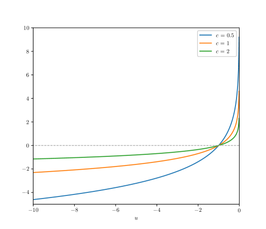
where is a barrier parameter that controls the accuracy of the approximation. Note that is convex, differentiable and increasing in . Figure 2.1 illustrates the function and the approximation , for several values of . As increases, the approximation becomes more accurate.
Substituting for in (2.5), we obtain the following approximation:
| (2.6) |
where , and the function with is known as the logarithmic barrier for the problem (1.1). Since our goal is to design a dynamical system capable of indirectly tracking the optimal solution of the original problem (1.1), it is essential to initialize the dynamical system at a point inside , i.e., . To circumvent this restriction, we introduce a nonnegative slack variable into the approximation problem (2.6) and reformulate it as follows:
| (2.7) |
where is an open and convex set that containing . For any , we can choose to ensure , meaning the initial condition lies within the “enlarged” feasible set . Let be the minimizer of (2.7). To simplify the problem, we define the function
Here, is twice differentiable and strongly convex [40]. Therefore, the approximation problem (2.7) is equivalent to
| (2.8) |
The optimal solution of (2.7) satisfies the optimality condition .
Next, we characterize the approximation error in terms of , , and the optimal dual variable .
Lemma 2.1
Proof: Define as
| (2.10) |
which is a perturbed version of the original optimization problem (1.1) after including the slack variable in the constraints. This problem coincides with the original problem (1.1) when . If is positive, it means that we have relaxed the -th inequality constraint. By perturbation and sensitivity analysis [3, Sec.5.6], we can establish the following inequality when ,
| (2.11) |
The left inequality is based on the fact that the feasible set is enlarged when , and hence, the optimal value does not increase. The right inequality follows directly from a sensitivity analysis of the original problem [3, Sec.5]. On the other hand, by replacing the indicator function in (2.10) with the log-barrier function , we obtain the bound [3, Sec.11]
| (2.12) |
Combining (2.11) and (2.12), using triangle inequality, we have
The proof is complete.
3 Continuous-time Dynamical System
In this section, we design a continuous-time dynamical system and analyze its convergence properties. We begin by deriving the dynamical system from the Bregman Lagrangian.
3.1 The Bregman Lagrangian
Borrowing ideas from Wibisono et al. [23, 26], define the Bregman Lagrangian as follows
| (3.1) |
where , , and represent position, velocity and time, respectively. The functions are smooth increasing functions of time that determine the weighting of the velocity, the potential function, and the overall damping of the Lagrangian. The ideal scaling conditions are given as follows
| (3.2) |
which are required in the stability analysis of continuous-time dynamical systems in the following paper. For the Bregman Lagrangian , denote by the action functional on curves . From Hamilton’s principle [41], finding the curve which minimizes the action functional is equivalent to finding a stationary point for the Euler-Lagrange equation, that is
| (3.3) |
Proposition 3.1
Proof. The partial derivatives of the Bregman Lagrangian can be weitten,
We also compute the time derivative of ,
Using the ideal scaling condition (3.2), the Euler-Lagrange equation given by
In the calculation, the terms involving are eliminated and the terms involving are simplified.
Remark 3.1
For the dynamical system (3.4), the solution must ensure that the argument of the logarithmic barrier function (2.8) remains positive. That is, for all , . In deed,
if exists such that , then is unbounded (singular) at the boundary of , which is impossible since the strong convexity of implies that is bounded for all . Thus, we must have that for all .
3.2 Convergence rates of the Continuous-time Dynamical System
In this subsection, we study the convergence of the continuous-time dynamical system given in Proposition 3.1. First, we show that the solution of the continuous-time dynamical system (3.4) exponentially converts to the approximate solution in (2.7) by employing Lyapunov function approach [42].
Lemma 3.1
Proof. Consider the following Lyapunov function
| (3.6) |
Observe that (3.6) is non-negative. since the function is convex, we have for all . The rest of the energy functional is positive due to for any . The time derivative of the Lyapunov functional is
Substitute (3.4) into the above formula, we have
where is the Bregman divergence of . By the ideal scaling conditions (3.2) and the nonnegativity of , we have . It follows that for all . This together with the definition of and the fact of yields
| (3.7) |
Furthermore, since is -strongly convex, and large enough, it follows that is -strongly convex for and so
| (3.8) |
In order to establish the convergence relationship between the solution generated by continuous-time dynamical system (3.4) and the optimal solution in (1.1), it is necessary to make the following assumptions about the barrier parameter , the slack variable and the optimal dual variable .
Assumption 3.1
For , assume that
-
(i)
is a time-dependent positive barrier function, i.e., ;
-
(ii)
is a nonnegative time-dependent slack function, i.e., ;
-
(iii)
the optimal dual variables satisfy .
Remark 3.2
Theorem 3.1
Proof: Under Assumption 3.1, by Lemmas 2.1 and 3.1, we can directly get . Next, we discuss the convergence rate. By the strong convexity of ,
It follows from that
| (3.9) |
Since is -smooth, for any , . Let and , we get
| (3.10) |
Combining (3.9) and (3.10) yields
By Assumption 3.1 and Lemma 2.1, one has . It follows that
By Lemma 3.1, we have
This completes the proof.
4 Discrete-time Algorithms
Wibisono et al. [23] pointed out that the numerical algorithms whose convergence rates match those of the underlying dynamical system cannot be easily obtained by using the naive numerical discretization method, and even the proposed discretization algorithm fails to converge. Therefore, it is meaningful to study the discrete-time algorithms.
In this section, we design several acceleration algorithms for the optimization problem (2.8) based on the Euler discretization [43] of dynamical system (3.4) and analyze the convergence of the proposed discrete-time algorithms using discrete-time Lyapunov functions. This ideal is inspired by Wilson et al. [26], which discussed various discretization schemes for the continuous-time dynamical system of unconstrained optimization. From now on, we assume that the first ideal scaling condition in (3.2) holds with equality, i.e., . In order to get the discretizations of continuous-time dynamical system (3.4), we first rewrite it as the following system of first-order equations
| (4.1) |
Next, we discretize and into sequences and with time step . That is, we make the identification and set
The explicit (forward) Euler discretization for and are defined as
The implicit (backward) Euler discretization for and are defined as
For the scaling parameters, we choose , and the discretizations as follows
4.1 Implicit Euler Discretization
In this subsection, we show that the implicit discretization of continuous-time dynamical system (4.1) can produce an acceleration algorithm whose convergence rate matches that of the underlying dynamical system.
By the implicit Euler discretization of and , the continuous-time dynamical system (4.1) can be discretized as follows
| (4.2) |
It is worth noting that (4.2) actually gives the optimality condition for a discrete-time algorithm, which is depicted in Algorithm 1.
The following theorem shows that the convergence behavior of Algorithm 1 by using discrete-time Lyapunov function.
Theorem 4.1
Suppose is -smooth. Define the discrete-time Lyapunov function
| (4.3) |
Then, under Assumption 3.1, and
Proof. From (4.3), we have
The second equality follows from the definition of , the third equality follows from (4.2), and the inequality follows from the convexity of and the fact of . Summing from to , we obtain . By definition of , one has . This together with the strong convexity of yields . For , by Assumption 3.1 and Lemma 2.1, one has . Since is strongly convex and smooth, using the same arguments as the proof of Theorem 3.1, we obtain
This completes the proof.
Remark 4.1
Theorem 4.1 establishes an acceleration gradient algorithm that matches the convergence rate of the dynamic system (4.1) by choosing an appropriate implicit discretization method. For constant . If , then achieve a polynomial convergence rate . If for some constant , then achieve an exponential convergence rate .
Remark 4.2
If for all , then Algorithm 1 can solve unconstrained convex optimization problems and achieve the best convergence rate.
4.2 Hybrid Euler Discretization with an Additional Sequence
Although Algorithm 1 is closely related to the continuous-time dynamical system (4.1) and has an optimal convergence rate, it involves an implicit update step (Step 3) which is pretty hard to solve in practice. Thus, it’s natural to consider whether computationally efficient algorithms can be derived using an explicit Euler discretization of one of the sequence. In this subsection, we present two algorithms using the aforementioned technique. One directly yields a gradient method, and the other, with an additional sequence, yields an accelerated gradient method that differs from the previous section.
First, we show Algorithm 2, which combines implicit and explicit Euler discretizations of dynamical system (4.1) with an additionally updating sequence.
Note that the additionally updating sequence can be seen as a step of mirror descent. The optimality condition of Algorithm 2 is given by
| (4.4) |
The following two Lemmas will be used in the sequel which plays an important role in our main results.
Lemma 4.1
[3, Sec.9] Given an initial point and a sublevel set . If is twice continuously differentiable, and strongly convex, i.e., for all . Then, there exists an such that for all .
Lemma 4.2
If is -strongly convex and is -smooth. Then where .
Proof. Since the optimal solution of (2.7) satisfies the optimality condition , by the smoothness of ,
By the strong convexity of , we have
Combining the two inequalities above yields By Remark 2.1, . It follows that .
By Lemma 4.1, we can assume without loss of generality that the smoothness coefficient of is . The following theorem shows that the convergence behavior of Algorithm 2 using a discrete-time Lyapunov function.
Theorem 4.2
Suppose is -strongly convex and is -smooth. Define the discrete-time Lyapunov function
| (4.5) |
Then, under Assumption 3.1, one has the error bound , where
In addition, if , and , then and
Proof. Using the Lyapunov function (4.5), we have
The second equality follows from the third equation of (4.4) and the first inequality follows from the properties of Bregman divergence, i.e., , . From Fenchel Young inequality, we have . Notice that
Then it follows that
From the first equation of (4.4) and , we have
This fact together with the convexity of yields the conclusion .
We now show that . By Lemma 4.1, there exists such that , . This upper bound on the Hessian implies for any ,
| (4.6) |
Let , plugging the second equation of (4.4) into the above inequality, we get . With the choices and , the inequality holds, this implies that . Since is strongly convex, and is strongly convex and smooth, using the same arguments as in the second part of the proof of Theorem 4.1, we can obtain that
| (4.7) |
Since is -strongly convex, by (4.6) and Lemma 4.2, . This together with the secod equation of (4.4) and (4.7) yield
Therefore, .
When , the acceleration gradient method (Algorithm 2) reduce to a gradient method, which explicit dircretization applied to the first equation of (4.1) and implicit discretization applied to the second equation of (4.1).
The discretization process is displayed in Algorithm 3. The optimality condition of Algorithm 3 is given by
| (4.8) |
Next, we can directly give the following corollary with the proof omitted.
Corollary 4.1
5 Numerical experiments
In this section, we solve an optimization problem with inequality constraints to illustrate the effectiveness of the accelerated gradient method in solving such problems. Specifically, we conduct numerical experiments to verify the acceleration performance and effectiveness of the algorithms derived from continuous-time dynamical system.
We consider the following quadratic optimization problem:
| (5.1) |
Next, we examine two distance-generating functions and their corresponding constraint sets :
-
•
Squared Euclidean norm: and for some constant .
-
•
Negative entropy: and .
In the following simulation, we show how to track the optimal solution using Algorithm 2. The augmented objective function (2.8) takes the form
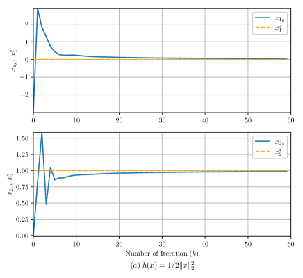
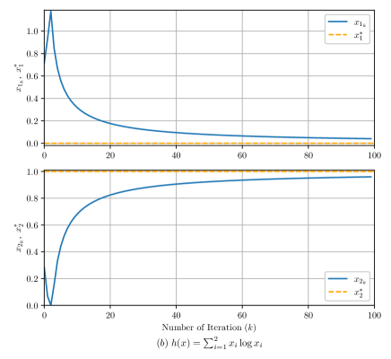
For the squared Euclidean norm distance, the radius of the Euclidean ball is set to be , the initial points and are randomly generated in , and . For the negative entropy distance, the initial points and are randomly generated in a -dimensional positive simplex, and . Moreover, using particular values, all conditions of Theorem 4.2 are satisfied.
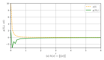
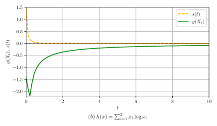
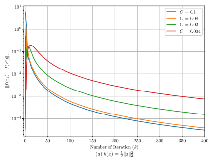
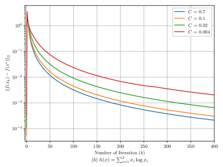
The trajectory of the solution , along with the optimal solution defined in (5.1), are shown in Figure 5.1. In detail, Figure 5.1(a) and Figure 5.1(b) show the results of the squared Euclidean norm distance and the negative entropy distance for the quadratic optimization problem, respectively. Figure 5.2(a) and Figure 5.2(b) display the time evolution of the constraint function and the nonnegative time-dependent slack function about the squared Euclidean norm distance and the negative entropy distance, respectively. We can see the state violates the constraint at . However, converges to the feasible set exponentially fast as the slack function vanishes exponentially. In Figure 5.3, we illustrate the performance of Algorithm 2 applied to (5.1), across various parameter settings for . We observe that the large is, the better Algorithm 2 performs.
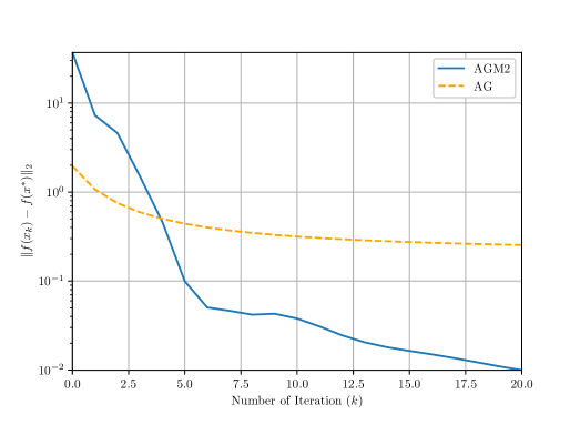
Finally, we consider and with the squared Euclidean norm distance. The radius of the Euclidean ball is set to be . For the stopping criterion, we choose . In Figure 5.4, we compare the performance of Algorithm 2 (AGM2) against Algorithm 3 (AG). We can clearly observe the effect that acceleration has on reducing the number of required iterations to obtain a certain accuracy. We noticed that, during the application of the Quasi-monotone method, the selection of with a relatively small magnitude can lead to a series of issues. Specifically, this small magnitude may lead to significant increases in rounding errors and cumulative errors, thereby weakening the stability of numerical calculations and resulting in oscillations characterized by repeated increases and decreases in error values.
6 Conclusions
In this paper, we investigated the accelerated gradient method for convex optimization problems with inequality constraints. Specifically, we approximate the inequality constrained convex optimization problem as an unconstrained optimization problem by employing the logarithmic barrier function. Under ideal scalar assumptions, we proposed a continuous-time dynamical system associated with the Bregman Lagrangian and derived its polynomial and exponential convergence rates based on the relevant parameter settings. Additionally, we developed several discrete-time algorithms by discretizing the continuous-time dynamical system, and obtained the fast convergence results matching that the underlying dynamical system. The numerical experiments demonstrated the acceleration performance and effectiveness of the proposed algorithms.
References
- [1] Beck, A. (2023). Introduction to nonlinear optimization: theory, algorithms, and applications with python and MATLAB (2nd ed.). Society for Industrial and Applied Mathematics, Philadelphia.
- [2] Boyd, S., Parikh, N., Chu, E., Peleato, B., Eckstein, J. (2011). Distributed optimization and statistical learning via the alternating direction method of multipliers. Foundations and Trends in Machine Learning, 3(1), 1-122.
- [3] Boyd, S., Vandenberghe, L. (2004). Convex optimization, Cambridge University Press, Cambridge.
- [4] Nocedal, J., Wright, S. (2006). Numerical optimization (2nd ed.). Springer Series in Operations Research and Financial Engineering. New York.
- [5] Bertsekas, D.P., Nedi, A., Ozdaglar, A.E. (2003). Convex analysis and optimization. Athena Scientific, Belmont.
- [6] Shor, N.Z., Kiwiel. K.C., Ruszczynski. A. (2012). Minimization methods for non-differentiable functions. Springer Series in Computational Mathematics, New York.
- [7] Esmaeili, H., Kimiaei, M. (2014). A new adaptive trust-region method for system of nonlinear equations. Applied Mathematical Modelling, 38(11-12), 3003-3015.
- [8] Chen, Y., Lan, G., Ouyang, Y. (2014). Optimal primal-dual methods for a class of saddle point problems. SIAM Journal on Optimization, 24(4), 1779-1814.
- [9] Nesterov, Y.E. (1983). A method of solving a convex programming problem with convergence rate . Soviet Mathematics Doklady, 27(2), 372-376.
- [10] Zhang, J., Luo, Z.Q. (2020). A proximal alternating direction method of multipliers for linearly constrained nonconvex minimization. SIAM Journal on Optimization, 30(3), 2272-2302.
- [11] Kong, W., Monteiro, R.D.C. (2023). An accelerated inexact dampened augmented Lagrangian method for linearly-constrained nonconvex composite optimization problems. Computational Optimization and Applications, 85, 509-545.
- [12] Nesterov, Y. (2005). Smooth minimization of non-smooth functions. Mathematical Programming, 103(1), 127-152.
- [13] Krichene, W., Bayen, A.M., Bartlett, P.L. (2015). Accelerated mirror descent in continuous and discrete time. Proceedings of the 28th International Conference on Neural Information Processing Systems, 2, pages 2845-2853.
- [14] Lan, G., Lu, Z., Monteiro, R.D.C. (2011). Primal-dual first-order methods with iteration-complexity for cone programming. Mathematical Programming, 126(1), 1-29.
- [15] Beck, A., Teboulle, M. (2009). A fast iterative shrinkage-thresholding algorithm for linear inverse problems. SIAM Journal on Imaging Sciences, 2(1), 183-202.
- [16] Lan, G. (2012). An optimal method for stochastic composite optimization. Mathematical Programming, 133(1-2), 365-397.
- [17] Liu, Y.F., Liu, X., Ma, S. (2019). On the nonergodic convergence rate of an inexact augmented Lagrangian framework for composite convex programming. Mathematics of Operations Research, 44(2), 632-650.
- [18] Ghadimi, S., Lan, G. (2012). Optimal stochastic approximation algorithms for strongly convex stochastic composite optimization I: A generic algorithmic framework. SIAM Journal on Optimization, 22(4), 1469-1492.
- [19] Ghadimi, S., Lan, G. (2015). Accelerated gradient methods for nonconvex nonlinear and stochastic programming. Mathematical Programming, 156(1), 59-99.
- [20] Su, W., Boyd, S., Candès, E.J. (2016). A differential equation for modeling Nesterov’s accelerated gradient method: Theory and insights. Journal of Machine Learning Research, 17, 1-43.
- [21] Shi, B., Du, S.S., Jordan, M.I., Su, W.J. (2021). Understanding the acceleration phenomenon via high-resolution differential equations. Mathematical Programming, 195, 1-70.
- [22] Nemirovski, A., Yudin, D.B. (1983). Problem complexity and method efficiency in optimization. Wiley & Sons, New York.
- [23] Wibisono, A., Wilson, A.C., Jordan, M.I. (2016). A variational perspective on accelerated methods in optimization. Proceedings of the National Academy of Sciences, 113(47), E7351-E7358.
- [24] Betancourt, M., Jordan, M.I., Wilson, A. (2018). On symplectic optimization. Arxiv preprint arXiv1802.03653.
- [25] Muehlebach, M., Jordan, M.I. (2021). Optimization with momentum: dynamical, control-theoretic, and symplectic perspectives. Journal of Machine Learning Research, 22, 1-50.
- [26] Wilson, A.C., Recht, B., Jordan, M.I. (2021). A Lyapunov analysis of accelerated methods in optimization. Journal of Machine Learning Research, 22, 1-34.
- [27] Chen, S., Shi, B., Yuan, Y.X. (2022). Revisiting the acceleration phenomenon via high-resolution differential equations. arXiv:2212.05700.
- [28] Wang, Y., Jia, Z., Wen, Z. (2021). Search direction correction with normalized gradient makes first-order methods faster. SIAM Journal on Scientific Computing. 43(5), A3184-A3211.
- [29] Luo, H., Chen, L. (2022). From differential equation solvers to accelerated first-order methods for convex optimization. Mathematical Programming. 195, 735-781.
- [30] Chen, L., Luo, H. (2019). First order optimization methods based on Hessian-driven Nesterov accelerated gradient flow. arXiv:1912.09276.
- [31] Bao, C.L., Chen, L., Li, J.H. (2023). The global R-linear convergence of nesterov’s accelerated gradient method with unknown strongly convex parameter. ArXiv:2308.14080.
- [32] Bao, C.L., Chen, L., Li, J.H., Shen, Z.W. (2024). Accelerated gradient methods with gradient restart: Global linear convergence. ArXiv: 2401.07672.
- [33] Fazlyab, M., Koppel, A., Ribeiro, A., Preciado, V.M. (2017). A variational approach to dual methods for constrained convex optimization. In Proceedings of the American Control Conference (pp. 5269-5275).
- [34] Zeng, X., Lei, J., Chen, J. (2022). Dynamical primal-dual accelerated method with applications to network optimization. arXiv:1912.03690.
- [35] Panier, E. R., Tits, A. L., Herskovits, J. N. (1988). A QP-free, globally convergent, locally superlinearly convergent algorithm for inequality constrained optimization. SIAM Journal on Control and Optimization. 26(4), 788-811.
- [36] Jian, J. B., Pan, H. Q., Tang, C. M., Li, J. L. (2015). A strongly sub-feasible primal-dual quasi interiorpoint algorithm for nonlinear inequality constrained optimization. Applied Mathematics and Computation. 266, 560-578.
- [37] Su, K., Ren, L. (2023). A modified nonmonotone filter QP-free method. Miskolc Mathematical Notes. 24(1), 457-471.
- [38] He, X., Hu, R., Fang, Y.P. (2021). Convergence rates of inertial primal-dual dynamical methods for separable convex optimization problems. SIAM Journal on Optimization. 59(5), 3278-3301.
- [39] Attouch, H., Chbani, Z., Fadili, J., Riahi, H. (2022). Fast convergence of dynamical ADMM via time scaling of damped inertial dynamics. Journal of Optimization Theory and Applications. 193(5), 704-736.
- [40] Fazlyab, M., Paternain, S., Preciado, V.M., Ribeiro, A. (2018). Prediction-correction interior-point method for time-varying convex optimization. IEEE Transactions on Automatic Control, 63(7), 1973-1986.
- [41] Bailey, C. (1982). Hamilton’s principle and the calculus of variations. Acta Mechanica, 44, 49-57.
- [42] Lyapunov, A.M. (1992). General problem of the stability of motion. International Journal of Control, 55(3), 531-773.
- [43] Kloeden, P.E., Platen, E. (1992). Higher-order implicit strong numerical schemes for stochastic differential equations. Journal of Statistical Physics, 66(3-4), 283-314.
- [44] Nesterov, Y., Shikhman, V. (2015). Quasi-monotone subgradient methods for nonsmooth convex minimization. Journal of Optimization Theory and Applications, 165(3), 917-940.