Transverse and longitudinal spin alignment from color fields in heavy ion collisions

Abstract

We analyze the spin alignment stemming from spin correlation of the quark and antiquark induced by background color fields in relativistic heavy ion collisions. The quark-coalescence equation relating the collision kernel of the vector-meson kinetic equation to spin alignment is expanded to the relativistic case. Focusing on the color-octet contribution, the spin alignment for $\phi$ mesons from glasma fields with momentum dependence is investigated, where the scenarios for different spin quantization axes are considered. Moreover, we qualitatively analyze the spin alignment from isotropic color fields in the quark gluon plasma phase for comparison. In particular, we propose that the experimental measurement of spin alignment along the beam direction, dubbed as the longitudinal spin alignment, could be useful to identify the dominance of longitudinal spin correlation potentially led by the glasma effect in high-energy nuclear collisions.

I Introduction

A large angular momentum can be generated in non-central heavy ion collisions, which may result in spin polarization of quark gluon plasma (QGP) through the spin-orbit interaction as theoretically proposed by Refs. [1, 2, 3]. The polarization of QGP is expected to be inherited by the polarization of produced hadrons, $\Lambda$ hyperons in practice, which has been indeed measured by the STAR Collaboration [4, 5] at BNL, ALICE Collaboration at CERN [6], and HADES Collaboration [7]. Theoretically, the global polarization of $\Lambda$ hyperons is successfully described by the polarization spectrum induced by thermal vorticity in a global thermodynamic equilibrium condition [8, 9, 10, 11, 12]. However, the follow-up observations of local spin polarization with momentum dependence along the longitudinal direction by STAR [5] disagree with the theoretical predictions based on the global equilibrium condition [11, 13, 14]. It is now understood that various contributions to spin polarization beyond the global equilibrium condition need to be considered.

In particular, the so-called thermal shear corrections as one of interaction-independent contributions in local equilibrium may play a crucial role [15, 16, 17] for local polarization according to the hydrodynamic simulations [18, 19, 20, 21]. Nonetheless, the numerical results from simulations are sensitive to the adopted approximations and chosen parameters [20, 21, 22]. In addition, further non-equilibrium contributions [15, 23, 24, 25, 26, 27, 28, 29, 30, 31, 32] or the influence from late-time magnetic fields [33] have been studied in recent years and a new observable, the helicity polarization along the momentum direction [34, 35, 36, 37], was proposed to distinguish different polarization mechanisms. See also Ref. [38] for a far-from-equilibrium kinetic-theory approach to address the local spin polarization. Despite the complexities, most of mechanisms for spin polarization are triggered by gradient corrections on hydrodynamic variables such as the temperature, fluid velocity, and chemical potentials. It is unclear how spin polarization phenomena in heavy ion collisions could have a deeper connection to the microscopic QCD properties in extreme conditions.

On the other hand, the spin alignment of vector mesons, characterized by the deviations of the ($00$)-component of the spin density matrix $\rho_{00}$ from its equilibrium value $1/3$ [39, 40], have been measured in heavy ion collisions  [41, 42, 43, 44]. As opposed to the relatively weak signal for spin polarization, the measured spin alignment is unexpectedly large and contradictory to the assumption of thermal equilibrium [45, 46] based on the spin coalescence model [2, 47]. It has been an open question and motivated a considerable number of theoretical studies  [48, 49, 50, 51, 52, 53, 54, 55, 56, 57, 58, 51, 52, 59, 60, 61, 62, 63, 64, 61, 65]. Among the possible mechanisms, Refs. [48, 51, 52, 54, 61, 59, 60] propose that the fluctuating strong-force fields in connection to QCD interaction could result in non-vanishing spin correlations between the quark and antiquark forming vector mesons via the quark coalescence [66, 67]. Due to fluctuating properties, such mechanisms giving rise to nonzero spin correlation will yield vanishing spin polarization for the $\Lambda$ hyperon mostly attributed to the spin polarization of the single constituted strange quark, which self-consistently explain the relatively small spin-polarization signal.

Notably, by considering the early-time spin correlation induced by chromo-electromagnetic fields dominantly along the beam direction in the glasma phase [68, 69] from the color glass condensate (CGC) effective theory [70, 71, 72, 73, 74], the magnitude of spin alignment for non-relativistic $\phi$ mesons is estimated in Ref. [60]. Despite the underlying simplifications and approximations, the estimated value may roughly explain the $\rho_{00}<1/3$ of $\phi$ mesons at small transverse momenta in LHC. The presence of glasma effect is however only expected in high-energy nuclear collisions such as at the top RHIC collision energy and LHC energies. In fact, the glasma phase as a pre-equilibrium state in heavy ion collisions is usually adopted as an initial condition for phenomenological studies [75], while the existence of such a phase itself has not been experimentally confirmed. Therefore, the spin-alignment signal may also serve as an alternative probe for such a pre-equilibrium state with saturated gluons. On the contrary, the late-time spin correlation is proposed to be led by fluctuating vector-meson fields for $\phi$ mesons [54], from which the global spin alignment data for $\phi$ mesons may be described in RHIC energies, whereas the strengths of such vector-meson fields cannot be estimated from a first principle. They are instead treated as fitting parameters. The alternative proposal for turbulent color fields also emphasizes the late-time spin correlation in the QGP phase [51], whereas the order of magnitude cannot be pin downed either.

Generically, there could exist multiple effects for spin alignment with sophisticated collision-energy, flavor, and centrality dependence. More detailed studies for spin alignment spectra depending on momenta may provide further information to disentangle different mechanisms. In this paper, we expand our previous study of the spin alignment for non-relativistic $\phi$ mesons from glasma fields or generally from background color fields in the quark coalescence scenarios [60] to the relativistic case and investigate the momentum dependence of $\rho_{00}$ with the choices of different spin quantization axes. In addition to the in-plane and out-of-plane spin alignment usually discussed in literature [54, 61], we further study the spin alignment along the beam direction. We will dub the former (in-plane and out-of-plane) and latter (beam) as the transverse and longitudinal spin alignment, respectively.

The paper is structured as follows: In Sec. II, we briefly review the derivation of axial Wigner functions dictating the spin polarization of quarks and antiquarks from the quantum kinetic theory (QKT) with background color fields. In Sec. III, we revisit the quark coalescence scenario delineated by the collision kernel of the kinetic theory of vector mesons and derive a more general expression, especially suitable for studying the glasma effect, beyond the non-relativistic approximation and equal-mass condition. The choices of different spin quantization axes are also discussed. In Sec. IV, we evaluate the spin alignment of $\phi$ mesons from the glasma effect and show the numerical results with momentum dependence. In Sec. V, we further analyze the spin alignment of $\phi$ mesons from color fields in QGP with an emphasis on qualitative features and the comparison with the results from glasma fields. Finally, we present conclusions and outlook in Sec VI. Some technical details have been relegated to the appendices.

Throughout this paper we use the mostly minus signature of the Minkowski metric $\eta^{\mu\nu}={\rm diag}(1,-1,-1,-1)$ and the completely antisymmetric tensor $\epsilon^{\mu\nu\rho\lambda}$ with $\epsilon^{0123}=1$. We introduce the notations $A^{(\mu}B^{\nu)}\equiv A^{\mu}B^{\nu}+A^{\nu}B^{\mu}$, $A^{[\mu}B^{\nu]}\equiv A^{\mu}B^{\nu}-A^{\nu}B^{\mu}$, and $\tilde{F}^{\mu\nu}\equiv\epsilon^{\mu\nu\alpha\beta}F_{\alpha\beta}/2$. Greek and roman indices are used for space-time and spatial components, respectively, unless otherwise specified.

II Spin transport of quarks with color fields

In this section, we briefly review the QKT for spin transport of quarks with color fields constructed in Refs. [51, 52] and the approximate solution for dynamical spin polarization obtained in Ref. [60, 59]. For spin transport, one may focus on the vector and axial-vector components of Wigner functions for massive fermions, $\mathcal{V}^{\mu}(p,x)$ and $\mathcal{A}^{\mu}(p,x)$, where the former and the latter are responsible for the particle-number and spin-polarization spectra, respectively. The dynamical evolution of $\mathcal{V}^{\mu}(p,x)$ and $\mathcal{A}^{\mu}(p,x)$ in phase space can then be tracked by utilizing the QKT for relativistic fermions [76, 77, 78, 79, 80, 81, 82, 83, 84, 85, 86] (see also a recent review  [87] and references therein) with further inclusion of the color degrees of freedom [51, 52, 88]. For quarks carrying color charges, they can be further decomposed into the color-singlet and color-octet components,

$$\mathcal{V}^{\mu}(p,x)=\mathcal{V}^{{\rm s}\mu}(p,x)I+\mathcal{V}^{a\mu}(p,x)\,t^{a},\quad\mathcal{A}^{\mu}(p,x)=\mathcal{A}^{{\rm s}\mu}(p,x)I+\mathcal{A}^{a\mu}(p,x)\,t^{a},$$ (1)

where $t^{a}$ are the SU$(N_{c})$ generators such that $[t^{a},t^{b}]=if^{abc}t^{c}$ and $\{t^{a},t^{b}\}=N_{c}^{-1}\delta^{ab}I+d^{abc}t^{c}$ and $I$ is the identity matrix in color space. Throughout this paper, we will use the superscripts ${\rm s}$ and $a$ to denotes the color-singlet and color-octet components for color objects, respectively. Due to the quantum nature of spin, we may adopt the power counting, $\mathcal{V}^{\mu}\sim\mathcal{O}(\hbar^{0})$ and $\mathcal{A}^{\mu}\sim\mathcal{O}(\hbar)$ in the $\hbar$ expansion as the gradient expansion in phase space [84], and focus on the leading-order contribution. Accordingly, for the vector Wigner functions, we have

$$\mathcal{V}^{{\rm s}\mu}(p,x)=2\pi\delta(p^{2}-m^{2})f^{\rm s}_{V}(p,x),\quad\mathcal{V}^{a\mu}(p,x)=2\pi\delta(p^{2}-m^{2})f^{a}_{V}(p,x)$$ (2)

where $f^{\rm s}_{V}(p,x)$ and $f^{a}_{V}(p,x)$ denote the color-singlet and color-octet distribution functions, respectively, and $m$ represents the quark mass. For the axial-vector Wigner functions, we have

$$\mathcal{A}^{{\rm s}\mu}(p,x) = 2\pi\Big{[}\delta(p^{2}-m^{2})\tilde{a}^{{\rm s}\mu}(p,x)+\frac{\hbar g}{2N_{c}}\delta^{\prime}(p^{2}-m^{2})p_{\nu}\tilde{F}^{a\mu\nu}f^{a}_{V}(p,x)\Big{]},$$

$$\mathcal{A}^{a\mu}(p,x) = 2\pi\Big{[}\delta(p^{2}-m^{2})\tilde{a}^{a\mu}(p,x)+\hbar g\delta^{\prime}(p^{2}-m^{2})p_{\nu}\Big{(}\tilde{F}^{a\mu\nu}f^{\rm s}_{V}(p,x)+\frac{d^{bca}}{2}\tilde{F}^{b\mu\nu}f^{c}_{V}(p,x)\Big{)}\Big{]},$$ (3)

where $g$ is the coupling constant of strong interaction, $\delta^{\prime}(x)\equiv\partial\delta(x)/\partial x$, and $\tilde{F}^{a\mu\nu}\equiv\epsilon^{\mu\nu\alpha\beta}F^{a}_{\alpha\beta}/2$ with $F^{a}_{\alpha\beta}$ being the field strength of color fields. Also, $\tilde{a}^{{\rm s}\mu}(p,x)$ and $\tilde{a}^{a\mu}(p,x)$ denote the color-singlet and color-octet effective spin four vector, respectively. We may further introduce the on-shell axial Wigner functions in connection to spin polarization spectra,

$$\mathcal{A}^{{\rm s}\mu}(\bm{p},x) \equiv \int\frac{dp_{0}}{2\pi}\mathcal{A}^{{\rm s}\mu}(p,x)=\frac{1}{2\epsilon_{\bm{p}}}\Big{[}\tilde{a}^{{\rm s}\mu}-\frac{\hbar}{4N_{c}}\tilde{F}^{a\mu\nu}\Big{(}\partial_{p\nu}f^{a}_{\rm V}-\frac{\epsilon_{\bm{p}}}{2}\partial_{p_{\perp}\nu}(f^{a}_{V}/\epsilon_{\bm{p}})\Big{)}\Big{]}_{p_{0}=\epsilon_{\bm{p}}},$$

$$\mathcal{A}^{a\mu}(\bm{p},x) \equiv \int\frac{dp_{0}}{2\pi}\mathcal{A}^{a\mu}(p,x)$$ (4)

$$= \frac{1}{2\epsilon_{\bm{p}}}\Big{[}\tilde{a}^{a\mu}-\frac{\hbar}{2}\tilde{F}^{a\mu\nu}\Big{(}\partial_{p\nu}f^{\rm s}_{V}-\frac{\epsilon_{\bm{p}}}{2}\partial_{p_{\perp}\nu}(f^{\rm s}_{V}/\epsilon_{\bm{p}})\Big{)}$$

$$-\frac{\hbar d^{bca}}{4}\tilde{F}^{b\mu\nu}\Big{(}\partial_{p\nu}f^{c}_{V}-\frac{\epsilon_{\bm{p}}}{2}\partial_{p_{\perp}\nu}(f^{c}_{V}/\epsilon_{\bm{p}})\Big{)}\Big{]}_{p_{0}=\epsilon_{\bm{p}}},$$

where $\epsilon_{\bm{p}}\equiv\sqrt{|\bm{p}|^{2}+m^{2}}$.

The dynamics of vector-charge distribution functions and effective spin four vector in phase space are governed by the coupled scalar kinetic equations (SKE),

$$p^{\rho}\Big{(}\partial_{\rho}f^{\rm s}_{V}+\frac{g}{2N_{c}}F^{a}_{\nu\rho}\partial_{p}^{\nu}f^{a}_{V}\Big{)}=\mathcal{C}_{\rm s},$$ (5)

$$p^{\rho}\Big{(}D_{\rho}f^{a}_{V}+gF^{a}_{\nu\rho}\partial_{p}^{\nu}f^{\rm s}_{V}+\frac{d^{bca}}{2}gF^{b}_{\nu\rho}\partial_{p}^{\nu}f^{c}_{V}\Big{)}=\mathcal{C}^{a}_{\rm o},$$ (6)

and axial kinetic equations (AKE) ,

$$p^{\rho}\partial_{\rho}\tilde{a}^{\rm s\mu}+\frac{g}{2N_{c}}\Big{(}p^{\rho}F^{a}_{\nu\rho}\partial_{p}^{\nu}\tilde{a}^{a\mu}+F^{a\nu\mu}\tilde{a}^{a}_{\nu}\Big{)}-\frac{\hbar}{4N_{c}}\epsilon^{\mu\nu\rho\sigma}p_{\rho}(\partial_{\sigma}gF^{a}_{\beta\nu})\partial_{p}^{\beta}f_{V}^{a}=\mathcal{C}^{\mu}_{\rm s},$$ (7)

$$p^{\rho}D_{\rho}\tilde{a}^{a\mu}+g\big{(}p^{\rho}F^{a}_{\nu\rho}\partial_{p}^{\nu}\tilde{a}^{\rm s\mu}+F^{a\nu\mu}\tilde{a}^{\rm s}_{\nu}\big{)}+\frac{d^{bca}}{2}g\big{(}p^{\rho}F^{b}_{\nu\rho}\partial_{p}^{\nu}\tilde{a}^{c\mu}+F^{b\nu\mu}\tilde{a}^{c}_{\nu}\big{)}$$

$$-\frac{\hbar}{2}\epsilon^{\mu\nu\rho\sigma}p_{\rho}(D_{\sigma}gF^{a}_{\beta\nu})\partial_{p}^{\beta}f_{V}^{\rm s}=\mathcal{C}^{a\mu}_{\rm o},$$ (8)

where $D_{\rho}O^{a}\equiv\partial_{\rho}O^{a}-gf^{bca}A^{b}_{\rho}O^{c}$ denotes the covariant derivative for an arbitrary color object $O^{a}$. Here we do not specify the collision terms explicitly. See Refs. [51, 52] for more detailed explanations of the theoretical framework.

For our purpose, we may focus on $\mathcal{A}^{a\mu}(\bm{p},x)$ responsible for the color-octet contribution to spin correlation. We first consider the dynamical spin polarization from $\tilde{a}^{a\mu}$ induced by space-time varying color fields obtained from Eq. (II). Following the perturbative approach in Ref. [60], one may drop the diffusion terms linear to $\tilde{a}^{{\rm s}\mu}$ and induced by color fields, whereby we approximate Eq. (II) as

$$p^{\rho}\partial_{\rho}\tilde{a}^{a\mu}-\frac{\hbar}{2}\epsilon^{\mu\nu\rho\sigma}p_{\rho}(\partial_{\sigma}gF^{a}_{\beta\nu})\partial_{p}^{\beta}f_{V}^{\rm s}=0,$$ (9)

where the collision term is also suppressed at weak coupling. One hence obtains the solution for dynamical polarization induced by color fields as

$$\tilde{a}^{a\mu}(p,x) = \frac{\hbar g}{2p_{0}}\int^{x_{0}}_{t_{\rm i}}dx^{\prime}_{0}\epsilon^{\mu\nu\rho\sigma}p_{\rho}\big{(}\partial_{x^{\prime}\sigma}F^{a}_{\beta\nu}(x^{\prime})\big{)}\partial_{p}^{\beta}f^{\rm s}_{V}(p,x^{\prime})|_{\text{c}},$$ (10)

where $|_{\text{c}}=\{x^{\prime i}_{\rm T}=x^{i}_{\rm T},x^{\prime i}_{\parallel}=x^{i}_{\parallel}-p^{i}(x_{0}-x^{\prime}_{0})/p_{0}\}$ with $x_{0}$ being the present time and $t_{\rm i}\leq x_{0}$ denotes the initial time for having a non-vanishing integrand. Here $V^{i}_{\rm T}$ and $V^{i}_{\parallel}$ represent the perpendicular and parallel components with respect to the spatial momentum $p^{i}$ for an arbitrary spatial vector $V^{i}$, respectively. We may express the chromo-electromagnetic fields in terms of a temporal vector $n^{\mu}=(1,\bm{0})$,

$$F^{a}_{\alpha\beta}=-\epsilon_{\mu\nu\alpha\beta}B^{a\mu}n^{\nu}+n_{\beta}E^{a}_{\alpha}-n_{\alpha}E^{a}_{\beta}.$$ (11)

By utilizing $\epsilon^{ijk}\partial_{j}E^{a}_{k}=\partial_{0}B^{ai}$ from the Bianchi identity $\partial_{\mu}\tilde{F}^{a\mu\nu}=0$ for Abelianized color fields and assuming $f^{\rm s}_{V}(p,x^{\prime})=f^{\rm s}_{V}(p_{0},x^{\prime}_{0})$ as an isotropic distribution in momentum and position space, Eq. (10) can be written as

$$\tilde{a}^{a\mu}(p,x) = \frac{\hbar g}{2p_{0}}\int^{x_{0}}_{t_{\rm i}}dx^{\prime}_{0}\big{(}p_{0}\partial_{x^{\prime}0}B^{ai}(x^{\prime})+\epsilon^{ijk}p_{k}\partial_{x^{\prime}0}E^{a}_{j}(x^{\prime})\big{)}\partial_{p}^{\beta}f^{\rm s}_{V}(p_{0},x^{\prime}_{0})|_{\text{c}}.$$ (12)

When the chromo-electromagnetic fields vary rapidly only in early times for $0\leq t_{\rm i}\leq x^{\prime}_{0}\leq t_{\rm f}$, one may neglect the temporal derivative upon $f^{\rm s}_{V}(p_{0},x^{\prime}_{0})$ and derive

$$\tilde{a}^{ai}(p,x)|_{x_{0}=t_{\rm f}} \approx -\frac{\hbar g}{2}\Big{[}\Big{(}B^{ai}(t_{\rm i})-\frac{\epsilon^{ijk}p_{j}E^{a}_{k}(t_{\rm i})}{p_{0}}\Big{)}\partial_{p0}f^{\rm s}_{V}(p_{0},t_{\rm i})$$ (13)

$$-\Big{(}B^{ai}(t_{\rm f})-\frac{\epsilon^{ijk}p_{j}E^{a}_{k}(t_{\rm f})}{p_{0}}\Big{)}\partial_{p_{0}}f^{\rm s}_{V}(p_{0},t_{\rm f})\Big{]}.$$

For the glasma effect on spin alignment proposed in Ref. [60], one may further drop the contributions from late-time fields by assuming $B^{ai}(t_{\rm f}),\,E^{ai}(t_{\rm f})\ll B^{ai}(t_{\rm i}),\,E^{ai}(t_{\rm i})$ for time-decreasing glasma fields. We shall regard $\tilde{a}^{a\mu}(p,x)|_{t_{\rm f}=t_{\rm th}}$ as the early-time polarization induced in the glamsa phase ending at $t_{\rm th}$ as the thermailzation time and the onset of the QGP phase. For $t>t_{\rm th}$, the glasma fields vanish and the collisional effect in QGP should result in the spin relaxation. Then one has to solve

$$p^{\rho}\partial_{\rho}\tilde{a}^{a\mu}=-\frac{p_{0}\tilde{a}^{a\mu}}{\tau^{\rm o}_{\rm R}},$$ (14)

under the relaxation-time approximation for the collision term, where $\tau^{\rm o}_{\rm R}$ represents a constant spin relaxation time characterizing the scattering effect. Here the corresponding solution reads

$$\tilde{a}^{a\mu}(x_{0})=\tilde{a}^{a\mu}(t_{\rm th})e^{-x_{0}/\tau^{\rm o}_{\rm R}}.$$ (15)

Neglecting the non-dynamical contribution corresponding to the part besides $\tilde{a}^{a\mu}$ in $\mathcal{A}^{ai}$ due to the absence of color fields in late times, we arrives at

$$\mathcal{A}^{ai}(\bm{p},x)\approx-\frac{\hbar g}{4\epsilon_{\bm{p}}}e^{-x_{0}/\tau^{\rm o}_{\rm R}}\bigg{[}B^{ai}(t_{\rm i})-\frac{\epsilon^{ijk}p_{j}E^{a}_{k}(t_{\rm i})}{\epsilon_{\bm{p}}}\bigg{]}\partial_{\epsilon_{\bm{p}}}f^{\rm s}_{V}(\epsilon_{\bm{p}},t_{\rm i})$$ (16)

for the glasma effect. Such an effect only depends on the color fields and quark distribution functions in the initial time albeit with the suppression from collisions.

On the other hand, we may instead consider the late-time effect for spin alignment stemming from chromo-electromagnetic fields in QGP as the soft thermal gluons (or turbulent color fields discussed in Ref. [51]), for which we may perturbatively approximate

$$\mathcal{A}^{ai}(\bm{p},x) \approx -\frac{\hbar g}{4\epsilon_{\bm{p}}}\bigg{[}B^{ai}(x_{0})\partial_{\epsilon_{\bm{p}}}+\frac{\epsilon^{ijk}p_{j}E^{a}_{k}(x_{0})}{2\epsilon_{\bm{p}}}\big{(}\partial_{\epsilon_{\bm{p}}}+\epsilon_{\bm{p}}^{-1}\big{)}\bigg{]}f^{\rm s}_{V}(\epsilon_{\bm{p}},x_{0}),$$ (17)

where the dynamical contribution from $\tilde{a}^{ai}$ is instead dropped. Both scenarios will be further investigated in this work.

III Polarized vector mesons from quark coalescence

III.1 Generalization of the coalescence scenario

In Ref. [60], the collision kernel for the quark-coalescence scenario, where a quark and an antiquark combine to form a vector meson thorough the postulated vector coupling, for the kinetic equation of vector mesons is obtained, whereas further simplification such as the non-relativistic approximation and equal mass of the quarks and antiquarks are applied to further simplify the calculation. Although the equal-mass condition is satisfied for $\phi$ mesons, the non-relativistic approximation actually violates the momentum conservation even in the rest frame of vector mesons. Such a violation is however not too severe by tuning the constituent quark mass to the value close to one half of the vector-meson mass. For accuracy and generality, in this subsection, we further calculate this collision kernel by lifting the equal-mass condition and non-relativistic approximation with particular forms of the axial Wigner functions for quarks and antiquarks.

As shown in Ref. [60], the polarization dependent distribution function of vector mesons, $f_{\lambda}(q,x)$, with momentum $q$ and negligible spatial dependence obtained from the quark coalescence scenario for dilute vector mesons can be approximated as

$$f_{\lambda}(q)\approx\frac{\Delta t}{E_{q}}g_{\phi}\,\mathcal{C}_{{\rm col},\lambda}(q),$$ (18)

where $g_{\phi}$ denotes the vector-coupling constant, $E_{q}=\sqrt{|\bm{q}|^{2}+M^{2}}$ with $M$ being the mass of vector mesons, and $\Delta t$ represents the coalescence time assumed to by sufficiently small. Here the subscript $\lambda=0,\pm 1$ corresponds to the polarization of the spin-one vector mesons. The normalized $00$-th component of the spin density matrix of vector mesons that characterizes its spin alignment can be obtained from

$$\rho_{00}(q)=\frac{\int d\Sigma\cdot qf_{0}(q,x)}{\int d\Sigma\cdot q\big{(}f_{0}(q,x)+f_{+1}(q,x)+f_{-1}(q,x)\big{)}},$$ (19)

where $\Sigma^{\mu}$ corresponds to a freeze-out hypersurface. The collision kernel for quark coalescence reads

$$\mathcal{C}_{{\rm col},\lambda}(q)=\int\frac{d^{3}k}{(2\pi)^{3}}\delta\big{(}q_{0}-\epsilon_{q}(\bm{q}/2+\bm{k})-\epsilon_{\bar{q}}(\bm{q}/2-\bm{k})\big{)}\tilde{\mathcal{C}}_{{\rm col},\lambda}(q,k),$$ (20)

where $\epsilon_{q/\bar{q}}(\bm{p})\equiv\sqrt{|\bm{p}|^{2}+m^{2}_{q/\bar{q}}}$ with $m_{q}$ and $m_{\bar{q}}$ being the mass of quarks and of antiquarks, respectively, and

$$\tilde{\mathcal{C}}_{{\rm col},\lambda}(q,k)$$

$$=N_{m}{\rm Tr_{c}}\Bigg{\{}\Bigg{[}\frac{f_{Vq}(\bm{p},x)f_{V\bar{q}}(\bm{p}^{\prime},x)}{\epsilon_{q}(\bm{p})\epsilon_{\bar{q}}(\bm{p}^{\prime})}-\frac{4}{m_{q}m_{\bar{q}}}\mathcal{A}_{q}(\bm{p},x)\cdot\mathcal{A}_{\bar{q}}(\bm{p}^{\prime},x)\Bigg{]}\Bigg{(}1-\frac{2|k\cdot\epsilon(\lambda,{\bm{q}})|^{2}}{N_{m}}\Bigg{)}$$

$$\quad-\frac{4}{m_{q}m_{\bar{q}}}\Bigg{[}2{\rm Re}\Big{(}\epsilon(\lambda,{\bm{q}})\cdot\mathcal{A}_{q}(\bm{p},x)\epsilon^{*}(\lambda,{\bm{q}})\cdot\mathcal{A}_{\bar{q}}(\bm{p}^{\prime},x)\Big{)}+\frac{2}{N_{m}}\Big{(}2k\cdot\mathcal{A}_{q}(\bm{p},x)k\cdot\mathcal{A}_{\bar{q}}(\bm{p}^{\prime},x)$$

$$\quad+2{\rm Re}\big{(}k\cdot\epsilon(\lambda,{\bm{q}})\mathcal{A}_{q}(\bm{p},x)\cdot\epsilon^{*}(\lambda,{\bm{q}})\big{)}k\cdot\mathcal{A}_{\bar{q}}(\bm{p}^{\prime},x)$$

$$\quad+2{\rm Re}\big{(}k\cdot\epsilon(\lambda,{\bm{q}})\mathcal{A}_{\bar{q}}(\bm{p}^{\prime},x)\cdot\epsilon^{*}(\lambda,{\bm{q}})\big{)}k\cdot\mathcal{A}_{q}(\bm{p},x)\Big{)}\Bigg{\}}\Bigg{|}_{p,p^{\prime}}$$ (21)

is explicitly expressed in terms the axial Wigner functions of quarks and antiquarks. Here $|_{p,p^{\prime}}=\{p=\frac{q}{2}+k,p^{\prime}=\frac{q}{2}-k\}$ for $p$ and $p^{\prime}$ being the momenta of quarks and antiquarks, respectively. Also, $\epsilon(\lambda,{\bm{q}})$ denotes the polarization four-vector for vector mesons and

$$N_{m}=\frac{1}{2}\big{(}M^{2}-(m_{q}+m_{\bar{q}})^{2}\big{)}.$$ (22)

We also use subscripts $q$ and $\bar{q}$ to represent the contributions from quarks nd antiquarks for the vector distribution functions and axial-vector Wigner functions. We then work in the vector-meson rest frame, $q^{\mu}=(M,{\bm{0}})$, such that $\epsilon^{\mu}(\lambda,0)=(0,\bm{\epsilon}_{\lambda})\equiv\epsilon_{\lambda}^{\mu}$. Accordingly, the onshell and kinematic conditions give rise to

$$k_{0}=\frac{m_{q}^{2}-m_{\bar{q}}^{2}}{2M},\quad|\bm{k}|=\tilde{k}\equiv\frac{1}{2M}\big{[}(m_{q}^{2}-m_{\bar{q}}^{2})^{2}+M^{4}-2M^{2}(m_{q}^{2}+m_{\bar{q}}^{2})\big{]}^{1/2},$$ (23)

and

$$\delta\big{(}q_{0}-\epsilon_{q}(\bm{q}/2+\bm{k})-\epsilon_{\bar{q}}(\bm{q}/2-\bm{k})\big{)}=\frac{\big{(}M^{4}-(m_{q}^{2}-m_{\bar{q}}^{2})^{2}\big{)}\delta\big{(}|\bm{k}|-\tilde{k}\big{)}}{8M^{3}\tilde{k}}.$$ (24)

In Ref. [60], the equal-mass condition $m_{q}=m_{\bar{q}}$ and non-relativistic approximation $M-(m_{q}+m_{\bar{q}})\ll M$ are further applied to simplify the explicit form of Eq. (LABEL:eq:SigmaVA) for the $k$ integral.

In order to conduct the $k$ integral without using the non-relativistic approximation, we instead introduce explicit forms of $\mathcal{A}_{q/\bar{q}}^{i}(\bm{p},x)$ and $\mathcal{A}_{q/\bar{q}}^{i}(\bm{p}^{\prime},x)$ based on the possible structures induced by color fields in light of Eqs. (16) and (17), the polarization along chromo-magnetic fields and the one perpendicular to the momentum and chromo-electric fields as the spin Hall effect. Let us now assume

$$\mathcal{A}_{q/\bar{q}}^{i}(\bm{p},x)|_{\bm{q}=0}=\mathcal{A}_{q/\bar{q}}^{(0)i}(|\bm{k}|,x)+k_{j}\mathcal{A}_{q/\bar{q}}^{(1)ij}(|\bm{k}|,x),\quad f_{Vq/\bar{q}}(\bm{p},x)|_{\bm{q}=0}=f_{Vq/\bar{q}}(|\bm{k}|,x),$$

$$\mathcal{A}_{q/\bar{q}}^{i}(\bm{p}^{\prime},x)|_{\bm{q}=0}=\mathcal{A}_{q/\bar{q}}^{(0)i}(|\bm{k}|,x)-k_{j}\mathcal{A}_{q/\bar{q}}^{(1)ij}(|\bm{k}|,x),\quad f_{Vq/\bar{q}}(\bm{p}^{\prime},x)|_{\bm{q}=0}=f_{Vq/\bar{q}}(|\bm{k}|,x),$$ (25)

with $\mathcal{A}_{q/\bar{q}}^{(1)ji}(|\bm{k}|,x)=-\mathcal{A}_{q/\bar{q}}^{(1)ij}(|\bm{k}|,x)$. On the other hand, due to the constraint $p_{\mu}\mathcal{A}_{q/\bar{q}}^{\mu}(\bm{p},x)=0$, we also have the relations,

$$\mathcal{A}_{q/\bar{q}}^{0}(\bm{p},x)|_{\bm{q}=0} = -\Big{(}p_{i}\mathcal{A}_{q/\bar{q}}^{i}(\bm{p},x)/p_{0}\Big{)}\Big{|}_{\bm{q}=0}=-\epsilon_{q}(\bm{k})^{-1}k_{i}\mathcal{A}_{q/\bar{q}}^{i}(\bm{p},x)|_{\bm{q}=0},$$

$$\mathcal{A}_{q/\bar{q}}^{0}(\bm{p}^{\prime},x)|_{\bm{q}=0} = -\Big{(}p^{\prime}_{i}\mathcal{A}_{q/\bar{q}}^{i}(\bm{p}^{\prime},x)/p^{\prime}_{0}\Big{)}\Big{|}_{\bm{q}=0}=\epsilon_{\bar{q}}(\bm{k})^{-1}k_{i}\mathcal{A}_{q/\bar{q}}^{i}(\bm{p}^{\prime},x)|_{\bm{q}=0}.$$ (26)

Note that $\mathcal{A}_{q/\bar{q}}^{0}(\bm{p},x)|_{\bm{q}=0}$ and $\mathcal{A}_{q/\bar{q}}^{0}(\bm{p}^{\prime},x)|_{\bm{q}=0}$ do not contain the contributions from $\mathcal{A}_{q/\bar{q}}^{(1)ij}(|\bm{k}|,x)$ due to its anti-symmetric property. We may then apply the relations,

$$k^{i}k^{j}\rightarrow|\bm{k}|^{2}\Big{[}\bar{z}^{2}\epsilon^{i}_{\lambda}\epsilon^{j}_{\lambda}-\frac{(1-\bar{z}^{2})}{2}\hat{\Theta}^{ij}_{\lambda}\Big{]},\quad\hat{\Theta}^{ij}_{\lambda}=\eta^{ij}+\epsilon^{i}_{\lambda}\epsilon^{j}_{\lambda},\quad\bar{z}=\frac{-k\cdot\epsilon_{\lambda}}{|\bm{k}|},$$ (27)

and

$$k^{i}k^{j}k^{l}k^{n}\rightarrow|\bm{k}|^{4}\hat{\Theta}^{ijln}_{\lambda},$$

$$\hat{\Theta}^{ijln}_{\lambda}=\Big{[}\bar{z}^{2}\epsilon^{i}_{\lambda}\epsilon^{j}_{\lambda}-\frac{(1-\bar{z}^{2})}{2}\hat{\Theta}^{ij}_{\lambda}\Big{]}\Big{[}\bar{z}^{2}\epsilon^{l}_{\lambda}\epsilon^{n}_{\lambda}-\frac{(1-\bar{z}^{2})}{2}\hat{\Theta}^{ln}_{\lambda}\Big{]}+(i\leftrightarrow l)+(i\leftrightarrow n),$$

$$\hat{\Theta}^{ijln}_{\lambda}\epsilon_{\lambda i}\epsilon_{\lambda j}=3\bar{z}^{4}\epsilon^{l}_{\lambda}\epsilon^{n}_{\lambda}-\frac{\bar{z}^{2}(1-\bar{z}^{2})}{2}\hat{\Theta}^{ln}_{\lambda}=-\frac{\bar{z}^{2}(1-\bar{z}^{2})}{2}\eta^{ln}_{\lambda}-\frac{\bar{z}^{2}(1-7\bar{z}^{2})}{2}\epsilon^{l}_{\lambda}\epsilon^{n}_{\lambda},$$ (28)

for $\epsilon_{\lambda}$ being real and drop the terms with odd powers of $\bm{k}$ when evaluating the integral.

Based on the complicated yet straightforward computations shown in Appendix. A, it is found

$$f_{\lambda} = \frac{\Delta t}{E_{q}}g_{\phi}N_{m}N_{c}^{2}C_{V}\bigg{\{}1-\frac{1}{\pi^{2}m_{q}m_{\bar{q}}C_{V}N_{c}^{2}}\bigg{[}\bigg{(}1-2C_{m}+\frac{\tilde{k}^{2}}{2\epsilon_{q\tilde{k}}\epsilon_{\bar{q}\tilde{k}}}\Big{(}1-\frac{2C_{m}}{3}\Big{)}+\frac{4k_{0}^{2}}{3\epsilon_{q\tilde{k}}\epsilon_{\bar{q}\tilde{k}}}\bigg{)}\eta^{ij}\big{\langle}\mathcal{A}_{qi}^{a(0)}\mathcal{A}_{\bar{q}j}^{a(0)}\big{\rangle}$$ (29)

$$+\bigg{(}2\Big{(}1-\frac{4C_{m}}{3}\Big{)}-\frac{16C_{m}\tilde{k}^{2}}{15\epsilon_{q\tilde{k}}\epsilon_{\bar{q}\tilde{k}}}\bigg{)}{\rm Re}\Big{(}\big{\langle}\epsilon_{\lambda}\cdot\mathcal{A}_{q}^{a(0)}\epsilon_{\lambda}\cdot\mathcal{A}_{\bar{q}}^{a(0)}\big{\rangle}\Big{)}+\frac{|\bm{k}|^{2}}{3}\Big{(}1-\frac{2C_{m}}{5}\Big{)}\big{\langle}\mathcal{A}_{qij}^{a(1)}\mathcal{A}_{\bar{q}}^{a(1)ij}\big{\rangle}$$

$$+\frac{|\bm{k}|^{2}}{6}\Big{(}1+\frac{32C_{m}}{5}\Big{)}{\rm Re}\Big{(}\big{\langle}\epsilon^{i}_{\lambda}\epsilon^{*j}_{\lambda}\mathcal{A}_{qil}^{a(1)}\mathcal{A}_{\bar{q}j}^{a(1)l}\big{\rangle}\Big{)}\bigg{]}\bigg{\}}_{|\bm{k}|=\tilde{k}},$$

where

$$C_{V}=\frac{1}{2\pi^{2}}\Big{(}1-\frac{2C_{m}}{3}\Big{)}\frac{f_{Vq}(\epsilon_{q\tilde{k}},x_{0})f_{V\bar{q}}(\epsilon_{\bar{q}\tilde{k}},x_{0})}{\epsilon_{q\tilde{k}}\epsilon_{\bar{q}\tilde{k}}}\Big{|}_{|\bm{k}|=\tilde{k}},$$ (30)

$$\epsilon_{q/\bar{q}\tilde{k}}\equiv\sqrt{\tilde{k}^{2}+m^{2}_{q/\bar{q}}}=\frac{1}{2M}\big{[}(m_{q/\bar{q}}^{2}-m_{\bar{q}/q}^{2})+M^{2}\big{]},$$ (31)

and

$$C_{m}\equiv\frac{\tilde{k}^{2}}{N_{m}}=\frac{1}{2}\left(1-\frac{(m_{q}-m_{\bar{q}})^{2}}{M^{2}}\right).$$ (32)

Here we have dropped $f^{a}_{Vq,\bar{q}}$-related terms as the higher-order corrections for the polarization independent part and simply denoted $f_{Vq,\bar{q}}=f^{\rm s}_{Vq,\bar{q}}$ for brevity. Despite the assumption for a particular form of the axial Wigner functions involved, Eq. (29) now serves as a general expression satisfying the momentum conservation and applicable for $m_{q}\neq m_{\bar{q}}$.

III.2 Applications to glasma fields

We will now apply the formalism derived above to the color-octet contribution for the spin correlation from glasma fields in Eq. (16). Now, taking $p^{\mu}=q^{\mu}/2+k^{\mu}$ in the vector-meson rest frame, one could read out

$$\mathcal{A}_{q}^{a(0)i}(|\bm{k}|,x) = -\frac{\hbar g}{4\epsilon_{\bm{k}}}e^{-x_{0}/\tau^{\rm o}_{\rm R}}B^{ai}(0)\partial_{\epsilon_{\bm{k}}}f_{Vq}(\epsilon_{\bm{k}},0),$$ (33)

$$\mathcal{A}_{q}^{a(1)ik}(|\bm{k}|,x) = -\frac{\hbar g\epsilon^{ijk}}{4\epsilon_{\bm{k}}^{2}}e^{-x_{0}/\tau^{\rm o}_{\rm R}}E^{a}_{j}(0)\partial_{\epsilon_{\bm{k}}}f_{Vq}(\epsilon_{\bm{k}},0),$$ (34)

where we have taken $t_{\rm i}=0$ for simplicity. Similar equations for $\mathcal{A}_{a\bar{q}}^{(0)i}(|\bm{k}|,x)$ and $\mathcal{A}_{a\bar{q}}^{(1)ik}(|\bm{k}|,x)$ with overall minus signs due to opposite color charges can be found. However, there exists a subtlety for the decomposition of $\mathcal{A}_{q}^{ai}({\bm{p}},x)|_{\bm{q}=0}$ into $\mathcal{A}_{q}^{a(0)i}(|\bm{k}|,x)$ and $\mathcal{A}_{q/\bar{q}}^{a(1)ik}(|\bm{k}|,x)$ above. In fact, the color fields here implicitly incorporate the momentum dependence. For instance, $B^{ai}(0)$ in Eq. (33) should be explicitly written as $B^{ai}(0,x^{i}_{\rm T},x^{i}_{\parallel}-k^{i}t_{\rm th}/p_{0})$, which implicitly depends on $k^{i}$, with $p_{0}=M/2+k_{0}$, where $x^{i}_{\rm T}$ and $x^{i}_{\parallel}$ denote the transverse and parallel components with $\bm{k}$, respectively. Similarly, for $\mathcal{A}_{a\bar{q}}^{(0)i}(|\bm{k}|,x)$, we will have the contribution from $B^{ai}(0,x^{i}_{\rm T},x^{i}_{\parallel}+k^{i}t_{\rm th}/p_{0})$. Nevertheless, we have to compute the color-field correlation to obtain the spin correlation. Based on the translational invariance, the color-field correlator like $\langle B^{ai}(0,\bm{x})B^{ai}(0,\bm{y})\rangle$ should only depend on $|\bm{x}-\bm{y}|\propto|\bm{k}|$. Therefore, the application of Eqs. (33) and (34) to Eq. (29) is still valid.

Denoting $f_{Vq/\bar{q}}(\epsilon_{q/\bar{q}\bm{k}},0)=f^{(0)}_{Vq/\bar{q}}(\epsilon_{q/\bar{q}\bm{k}})$ for short and inserting Eqs. (33) and (34) into Eq. (29), we obtain

$$f_{\lambda} = \frac{\Delta t}{E_{q}}g_{\phi}N_{m}N_{c}^{2}C_{V}\bigg{\{}1-\frac{\hbar^{2}g^{2}C_{A}}{\pi^{2}m_{q}m_{\bar{q}}C_{V}N_{c}^{2}}\bigg{[}C_{B1}\sum_{j=x,y,z}\chi_{B}^{jj}+C_{B2}{\rm Re}\Big{(}\epsilon_{\lambda i}\epsilon^{*}_{\lambda j}\chi_{B}^{ij}\Big{)}$$ (35)

$$+C_{E1}\sum_{j=x,y,z}\chi_{E}^{jj}+C_{E2}{\rm Re}\big{(}\epsilon_{\lambda i}\epsilon^{*}_{\lambda j}\chi^{ij}_{E}\big{)}\bigg{]}\bigg{\}}_{|\bm{k}|=\tilde{k}},$$

where

$$C_{A}=\frac{(\partial_{\epsilon_{q\tilde{k}}}f^{(0)}_{qV})(\partial_{\epsilon_{\bar{q}\tilde{k}}}f^{(0)}_{\bar{q}V})}{16\epsilon_{q\tilde{k}}\epsilon_{\bar{q}\tilde{k}}}e^{-2x_{0}/\tau^{\rm o}_{\rm R}},$$ (36)

and

$$\chi_{B}^{ij} = \big{\langle}B^{ai}(0,\bm{x}+\bm{k}t^{\rm th}/p_{+})B^{aj}(0,\bm{x}-\bm{k}t^{\rm th}/p_{-})\big{\rangle},$$

$$\chi_{E}^{ij} = \big{\langle}E^{ai}(0,\bm{x}+\bm{k}t^{\rm th}/p_{+})E^{aj}(0,\bm{x}-\bm{k}t^{\rm th}/p_{-})\big{\rangle},$$ (37)

as functions of $|\bm{k}|=\tilde{k}$ and $p_{\pm}=(M^{2}\pm(m_{q}^{2}-m_{\bar{q}}^{2}))/(2M)$. Here we have utilized

$$\big{\langle}\mathcal{A}_{qij}^{a(1)}\mathcal{A}_{\bar{q}}^{a(1)ij}\big{\rangle}=-\frac{2C_{A}}{\epsilon_{q\tilde{k}}\epsilon_{\bar{q}\tilde{k}}}\sum_{j=x,y,z}\chi^{jj}_{E}$$ (38)

and

$${\rm Re}\Big{(}\big{\langle}\epsilon^{i}_{\lambda}\epsilon^{*j}_{\lambda}\mathcal{A}_{qil}^{a(1)}\mathcal{A}_{\bar{q}j}^{a(1)l}\big{\rangle}\Big{)}=\frac{C_{A}}{\epsilon_{q\tilde{k}}\epsilon_{\bar{q}\tilde{k}}}\Big{(}\sum_{j=x,y,z}\chi^{jj}_{E}-{\rm Re}\big{(}\epsilon_{\lambda i}\epsilon^{*}_{\lambda j}\chi^{ij}_{E}\big{)}\Big{)}.$$ (39)

The related coefficients explicitly read

$$C_{B1}=1-2C_{m}+\frac{\lambda_{\tilde{k}}}{2}\Big{(}1-\frac{2C_{m}}{3}\Big{)}+\frac{4\lambda_{k_{0}}}{3},\quad C_{B2}=-2\Big{(}1-\frac{4C_{m}}{3}\Big{)}+\frac{16C_{m}\lambda_{\tilde{k}}}{15},$$

$$C_{E1}=-\frac{1}{2}\Big{(}1-\frac{8C_{m}}{3}\Big{)}\lambda_{\tilde{k}},\quad C_{E2}=-\frac{1}{6}\Big{(}1+\frac{32C_{m}}{5}\Big{)}\lambda_{\tilde{k}},$$

where

$$\lambda_{\tilde{k}}\equiv\frac{\tilde{k}^{2}}{\epsilon_{q\tilde{k}}\epsilon_{\bar{q}\tilde{k}}} = \frac{\big{(}M^{2}-(m_{q}+m_{\bar{q}})^{2}\big{)}\big{(}M^{2}-(m_{q}-m_{\bar{q}})^{2}\big{)}}{M^{4}-(m_{q}^{2}-m_{\bar{q}}^{2})^{2}},$$

$$\lambda_{k_{0}}\equiv\frac{k_{0}^{2}}{\epsilon_{q\tilde{k}}\epsilon_{\bar{q}\tilde{k}}} = \frac{(m_{q}^{2}-m_{\bar{q}}^{2})^{2}}{M^{4}-(m_{q}^{2}-m_{\bar{q}}^{2})^{2}}.$$ (40)

When taking $M\approx m_{q}+m_{\bar{q}}$ and $m_{q}\approx m_{\bar{q}}$, it is found $\lambda_{\tilde{k}}\approx 0$ and $\lambda_{k_{0}}\approx 0$ along with $C_{m}\approx 1/2$, respectively, which correspond to the approximation and condition adopted in Ref. [60].

III.3 Spin quantization axes

Spin alignment characterized by $\rho_{00}$ depends on the choice of a spin quantization axis. In heavy ion collision, it is usually chosen to be the direction perpendicular to the reaction plane as the direction along the total angular momentum, known as the ”out-of-plane” spin alignment. For the coordinates in this paper, we will assign $\hat{z}$ as the beam direction and $\hat{y}$ as the angular-momentum direction perpendicular to the reaction plane. Consequently, by setting

$$\bm{\epsilon}_{0}=(0,1,0),\quad\bm{\epsilon}_{+1}=-\frac{1}{\sqrt{2}}(i,0,1),\quad\bm{\epsilon}_{-1}=\frac{1}{\sqrt{2}}(-i,0,1),$$ (41)

we derive

$$f_{0} = \frac{\Delta t}{E_{q}}g_{\phi}N_{m}N_{c}^{2}C_{V}\bigg{[}1-\frac{\hbar^{2}g^{2}C_{A}}{\pi^{2}m_{q}m_{\bar{q}}C_{V}N_{c}^{2}}\big{(}C_{B1}\sum_{j=x,y,z}\chi_{B}^{jj}+C_{B2}\chi_{B}^{yy}$$ (42)

$$+C_{E1}\sum_{j=x,y,z}\chi_{E}^{jj}+C_{E2}\chi^{yy}_{E}\big{)}\bigg{]}_{|\bm{k}|=\tilde{k}}$$

and

$$f_{\pm 1} = \frac{\Delta t}{E_{q}}g_{\phi}N_{m}N_{c}^{2}C_{V}\bigg{[}1-\frac{\hbar^{2}g^{2}C_{A}}{\pi^{2}m_{q}m_{\bar{q}}C_{V}N_{c}^{2}}\bigg{(}C_{B1}\sum_{j=x,y,z}\chi_{B}^{jj}+\frac{C_{B2}}{2}(\chi_{B}^{xx}+\chi_{B}^{zz})$$ (43)

$$+C_{E1}\sum_{j=x,y,z}\chi_{E}^{jj}+\frac{C_{E2}}{2}(\chi^{xx}_{E}+\chi^{zz}_{E})\bigg{)}\bigg{]}_{|\bm{k}|=\tilde{k}}.$$

In principle, when calculating $\rho_{00}(q)$ from Eq. (19), we have to integrate $f_{\lambda}$ over $d\Sigma\cdot q$, while the integral leads to just a trivial overall prefactor when neglecting the spatial dependence of $f_{\lambda}$. Nevertheless, $f_{\lambda}$ still depend on time and we may take $x_{0}=t_{\rm eq}$ as the time at the freeze-out hypersurface for chemical (or more precisely spin) equilibrium. Consequently, the out-of-plane spin alignment is given by

$$\rho^{\rm o}_{00}(q) = \frac{1-C_{g}\big{[}\big{(}C_{B1}+C_{B2}\big{)}\chi^{yy}_{B}+C_{B1}(\chi^{xx}_{B}+\chi^{zz}_{B}\big{)}+\big{(}C_{E1}+C_{E2}\big{)}\chi^{yy}_{E}+C_{E1}(\chi^{xx}_{E}+\chi^{zz}_{E}\big{)}\big{]}_{|\bm{k}|=\tilde{k}}}{3-C_{g}\big{[}\big{(}3C_{B1}+C_{B2}\big{)}\chi_{B}+\big{(}3C_{E1}+C_{E2}\big{)}\chi_{E}\big{]}_{|\bm{k}|=\tilde{k}}}$$

from Eq. (19), where

$$C_{g}=\frac{\hbar^{2}g^{2}C_{A}}{\pi^{2}m_{q}m_{\bar{q}}C_{V}N_{c}^{2}}\Big{|}_{x_{0}=t_{\rm eq}},\quad\chi_{B,E}=\sum_{j=x,y,z}\chi^{jj}_{B,E}.$$ (45)

For small spin correlations, $\chi^{jj}_{B}(t^{\rm th})\ll 1$, $\rho^{\rm o}_{00}(q)$ reduces to

$$\rho^{\rm o}_{00}(q)\approx\frac{1}{3}\bigg{[}1+\frac{1}{3}C_{g}\Big{(}C_{B2}\big{(}\chi^{xx}_{B}+\chi^{zz}_{B}-2\chi^{yy}_{B}\big{)}+C_{E2}\big{(}\chi^{xx}_{E}+\chi^{zz}_{E}-2\chi^{yy}_{E}\big{)}\Big{)}\bigg{]}_{|\bm{k}|=\tilde{k}}.$$ (46)

Furthermore, when choosing the helicity frame such that the spin quantization axis is along the momentum direction of the vector meson, we can also read out the expression of $\rho^{\rm h}_{00}$ from Eq. (III.3),

$$\rho^{\rm h}_{00}(q) = \frac{1-C_{g}\big{[}\big{(}C_{B1}+C_{B2}\big{)}\chi^{\hat{q}}_{B}+C_{B1}(\chi_{B}-\chi^{\hat{q}}_{B}\big{)}+\big{(}C_{E1}+C_{E2}\big{)}\chi^{\hat{q}}_{E}+C_{E1}(\chi_{E}-\chi^{\hat{q}}_{E}\big{)}\big{]}_{|\bm{k}|=\tilde{k}}}{3-C_{g}\big{[}\big{(}3C_{B1}+C_{B2}\big{)}\chi_{B}+\big{(}3C_{E1}+C_{E2}\big{)}\chi_{E}\big{]}_{|\bm{k}|=\tilde{k}}},$$

where $\chi^{\hat{q}}_{B,E}=\hat{q}_{i}\hat{q}_{j}\chi^{ij}_{B,E}$. The expression in the helicity frame is obtained by making the replacements, $\chi^{yy}_{B,E}\rightarrow\chi^{\hat{q}}_{B,E}$ and $\chi^{xx}_{B,E}+\chi^{zz}_{B,E}\rightarrow\chi_{B,E}-\chi^{\hat{q}}_{B,E}$, in Eq. (III.3). Notably, when we average the momentum directions by taking $\chi^{\hat{q}}_{B,E}\rightarrow\chi_{B,E}/3$, it is found $\rho^{\rm h}_{00}(q)\rightarrow 1/3$.

On the other hand, one may alternatively choose the beam direction as the spin quantization axis. In such a case, one can simply make the replacements, $\chi^{yy}_{B,E}\rightarrow\chi^{zz}_{B,E}$, $\chi^{zz}_{B,E}\rightarrow\chi^{xx}_{B,E}$, and $\chi^{xx}_{B,E}\rightarrow\chi^{yy}_{B,E}$ in Eq. (III.3). We hence obtain

$$\rho^{\rm b}_{00}(q) = \frac{1-C_{g}\big{[}\big{(}C_{B1}+C_{B2}\big{)}\chi^{zz}_{B}+C_{B1}(\chi^{xx}_{B}+\chi^{yy}_{B}\big{)}+\big{(}C_{E1}+C_{E2}\big{)}\chi^{zz}_{E}+C_{E1}(\chi^{xx}_{E}+\chi^{yy}_{E}\big{)}\big{]}_{|\bm{k}|=\tilde{k}}}{3-C_{g}\big{[}\big{(}3C_{B1}+C_{B2}\big{)}\chi_{B}+\big{(}3C_{E1}+C_{E2}\big{)}\chi_{E}\big{]}_{|\bm{k}|=\tilde{k}}}$$

as the master equation for the ”longitudinal” spin alignment. Analogously, we may also consider the spin quantization axis along the $\hat{x}$ direction as for the ”in-plane” spin alignment, for which we make the replacements, $\chi^{yy}_{B,E}\rightarrow\chi^{xx}_{B,E}$, $\chi^{zz}_{B,E}\rightarrow\chi^{yy}_{B,E}$, and $\chi^{xx}_{B,E}\rightarrow\chi^{zz}_{B,E}$ in Eq. (III.3). It is found

$$\rho^{\rm i}_{00}(q)=\frac{1-C_{g}\big{[}\big{(}C_{B1}+C_{B2}\big{)}\chi^{xx}_{B}+C_{B1}(\chi^{yy}_{B}+\chi^{zz}_{B}\big{)}+\big{(}C_{E1}+C_{E2}\big{)}\chi^{xx}_{E}+C_{E1}(\chi^{yy}_{E}+\chi^{zz}_{E}\big{)}\big{]}_{|\bm{k}|=\tilde{k}}}{3-C_{g}\big{[}\big{(}3C_{B1}+C_{B2}\big{)}\chi_{B}+\big{(}3C_{E1}+C_{E2}\big{)}\chi_{E}\big{]}_{|\bm{k}|=\tilde{k}}}.$$

IV Spin alignment from glasma

IV.1 Correlations of glasma fields

We may now estimate the spin alignment induced by color fields from the glasma following the similar setup in Ref. [60] to evaluate $\chi^{ij}_{B/E}$. From now on, we set $\hbar=1$. In such a case, only the correlations between longitudinal color fields parallel to the beam direction exist, which take the form [89]

$$\langle E^{az}(t,x_{\perp})E^{az}(t,y_{\perp})\rangle_{t=0} \approx \frac{1}{2}g^{2}N_{c}(N_{c}^{2}-1)\Omega_{+}(x_{\perp},y_{\perp}),$$ (50)

$$\langle B^{az}(t,x_{\perp})B^{az}(t,y_{\perp})\rangle_{t=0} \approx \frac{1}{2}g^{2}N_{c}(N_{c}^{2}-1)\Omega_{-}(x_{\perp},y_{\perp}),$$ (51)

where we use the subscripts $\perp$ here to represent the transverse components. We may further adopt the Golec-Biernat Wüsthoff (GBW) dipole distribution such that [90, 89]

$$\Omega_{\pm}(u_{\perp},v_{\perp})=\Omega(u_{\perp},v_{\perp})=\frac{Q_{s}^{4}}{g^{4}N_{c}^{2}}\left(\frac{1-e^{-Q_{s}^{2}|u_{\perp}-v_{\perp}|^{2}/4}}{Q_{s}^{2}|u_{\perp}-v_{\perp}|^{2}/4}\right)^{2},$$ (52)

where $Q_{s}$ denotes the saturation momentum. Accordingly, it is found

$$\chi^{zz}_{B}=\chi^{zz}_{E}=\chi_{\rm GBW}\equiv\frac{Q_{s}^{4}(N_{c}^{2}-1)}{2g^{2}N_{c}}\left(\frac{1-e^{-Q_{s}^{2}\tilde{k}^{2}(t^{\rm th}\lambda_{m})^{2}/4}}{Q_{s}^{2}\tilde{k}^{2}(t^{\rm th}\lambda_{m})^{2}/4}\right)^{2},$$ (53)

where $\lambda_{m}=|p_{+}^{-1}+p_{-}^{-1}|=4M^{3}/(M^{4}-(m_{q}^{2}-m_{\bar{q}}^{2})^{2})$. Now, due to the dominance of longitudinal color fields and Eq. (53), Eq. (III.3) reduces to

$$\rho^{\rm o}_{00}(q) \approx \frac{1-C_{g}\big{[}C_{B1}+C_{E1}\big{]}\chi^{zz}_{B}}{3-C_{g}\big{[}\big{(}3C_{B1}+C_{B2}\big{)}+\big{(}3C_{E1}+C_{E2}\big{)}\big{]}\chi^{zz}_{B}}.$$ (54)

Except for the color-field correlators, $\rho^{\rm o}_{00}(q)$ also depends on the quark and antiquark distribution functions at the initial time and the freeze-out hypersurface. As adopted in Ref. [60], we postulate

$$f^{(0)}_{Vq/\bar{q}}(\epsilon_{q/\bar{q}\bm{k}})=\Big{(}{\rm exp}\big{(}\sqrt{|\bm{k}|^{2}+m^{2}_{q/\bar{q}}}/Q_{s}\big{)}+1\Big{)}^{-1}$$ (55)

as the non-equilibrium distribution functions of quarks and antiquakrs in the glasma state and hence $\partial_{\epsilon_{q/\bar{q}\bm{k}}}f^{(0)}_{Vq/\bar{q}}=-Q_{s}^{-1}f^{(0)}_{Vq/\bar{q}}(1-f^{(0)}_{Vq/\bar{q}})$ for $C_{A}$ in Eq. (36). On the other hand, the quark and antiquark distribution functions, $f_{Vq/\bar{q}}(\epsilon_{q/\bar{q}\bm{k}},t_{\rm th})$ in $C_{V}$, come from those in the QGP phase at late times. Consequently, one may take

$$f_{Vq/\bar{q}}(\epsilon_{q/\bar{q}\bm{k}},t_{\rm th})=\Big{(}{\rm exp}\big{(}\sqrt{|\bm{k}|^{2}+m^{2}_{q/\bar{q}}}/T_{\rm eq}\big{)}+1\Big{)}^{-1}$$ (56)

as the equilibrium distribution functions with the freeze-out temperature $T_{\rm eq}$ to evaluate $C_{V}$ in Eq. (30). In such a case, the competition between the spin-relaxation factor $e^{-2t_{\rm eq}/\tau^{\rm o}_{\rm R}}$ and the ratio of $f^{(0)}_{Vq/\bar{q}}(\epsilon_{q/\bar{q}\bm{k}})$ to $f_{Vq/\bar{q}}(\epsilon_{q/\bar{q}\bm{k}},t_{\rm th})$ also becomes crucial for the magnitude of spin alignment.

IV.2 Retrieving momentum dependence

As also discussed in Ref. [60], to retrieve the momentum dependence of $\rho_{00}$, we could rewrite $B^{ai}_{\rm r}$ and $E^{ai}_{\rm r}$ as the color fields in the rest frame in terms of those in the lab frame through

$$B^{ai}_{\rm r} = \gamma(B^{ai}+\epsilon^{ijk}v_{j}E^{a}_{k})-(\gamma-1){\bm{B}}^{a}\cdot\hat{{\bm{v}}}\hat{v}^{i},$$

$$E^{ai}_{\rm r} = \gamma(E^{ai}-\epsilon^{ijk}v_{j}B^{a}_{k})-(\gamma-1){\bm{E}}^{a}\cdot\hat{{\bm{v}}}\hat{v}^{i},$$ (57)

where $\gamma=1/\sqrt{1-|{\bm{v}}|^{2}}$ with $v^{i}=q^{i}/\sqrt{|\bm{q}|^{2}+M^{2}}$ and $\hat{v}^{i}=v^{i}/|\bm{v}|$. By dropping the correlations between a chromo-magnetic field and an electric one and those between color fields along different directions, we accordingly find

$$\langle B^{ai}_{\rm r}B^{ai}_{\rm r}\rangle = \gamma^{2}\big{(}\langle B^{ai}B^{ai}\rangle+\epsilon^{ijk}v_{j}\epsilon^{ij^{\prime}k^{\prime}}v_{j^{\prime}}\langle E^{a}_{k}E^{a}_{k^{\prime}}\rangle\big{)}$$

$$-2\gamma(\gamma-1)\langle B^{ai}B^{ai}\rangle\hat{v}_{i}^{2}+(\gamma-1)^{2}\hat{v}_{i}^{2}\sum_{j=x,y,z}\langle B^{aj}B^{aj}\rangle$$

and

$$\langle E^{ai}_{\rm r}E^{ai}_{\rm r}\rangle = \gamma^{2}\big{(}\langle E^{ai}E^{ai}\rangle+\epsilon^{ijk}v_{j}\epsilon^{ij^{\prime}k^{\prime}}v_{j^{\prime}}\langle B^{a}_{k}B^{a}_{k^{\prime}}\rangle\big{)}$$ (59)

$$-2\gamma(\gamma-1)\langle E^{ai}E^{ai}\rangle\hat{v}_{i}^{2}+(\gamma-1)^{2}\hat{v}_{i}^{2}\sum_{j=x,y,z}\langle E^{aj}E^{aj}\rangle.$$

For brevity, we do not show the spatial dependence of all the equal-time correlators at $t=0$ above explicitly. Considering the dominance of longitudinal chromo-fields in the early time, we approximate

$$\langle B^{ax}_{\rm r}B^{ax}_{\rm r}\rangle \approx \gamma^{2}v_{y}^{2}\langle E^{az}E^{az}\rangle+(\gamma-1)^{2}\hat{v}_{x}^{2}\langle B^{az}B^{az}\rangle,$$

$$\langle B^{ay}_{\rm r}B^{ay}_{\rm r}\rangle \approx \gamma^{2}v_{x}^{2}\langle E^{az}E^{az}\rangle+(\gamma-1)^{2}\hat{v}_{y}^{2}\langle B^{az}B^{az}\rangle,$$

$$\langle B^{az}_{\rm r}B^{az}_{\rm r}\rangle \approx \big{(}\gamma^{2}+(1-\gamma^{2})\hat{v}_{z}^{2}\big{)}\langle B^{az}B^{az}\rangle,$$ (60)

and

$$\langle E^{ax}_{\rm r}E^{ax}_{\rm r}\rangle \approx \gamma^{2}v_{y}^{2}\langle B^{az}B^{az}\rangle+(\gamma-1)^{2}\hat{v}_{x}^{2}\langle E^{az}E^{az}\rangle,$$

$$\langle E^{ay}_{\rm r}E^{ay}_{\rm r}\rangle \approx \gamma^{2}v_{x}^{2}\langle B^{az}B^{az}\rangle+(\gamma-1)^{2}\hat{v}_{y}^{2}\langle E^{az}E^{az}\rangle,$$

$$\langle E^{az}_{\rm r}E^{az}_{\rm r}\rangle \approx \big{(}\gamma^{2}+(1-\gamma^{2})\hat{v}_{z}^{2}\big{)}\langle E^{az}E^{az}\rangle.$$ (61)

When adopting the GBW distribution, we have $\langle B^{az}B^{az}\rangle=\langle E^{az}E^{az}\rangle$ and accordingly

$$\chi^{xx}_{B}(q) = \chi^{xx}_{E}(q)=\big{(}\gamma^{2}v_{y}^{2}+(\gamma-1)^{2}\hat{v}_{x}^{2}\big{)}\chi_{\rm GBW},$$

$$\chi^{yy}_{B}(q) = \chi^{yy}_{E}(q)=\big{(}\gamma^{2}v_{x}^{2}+(\gamma-1)^{2}\hat{v}_{y}^{2}\big{)}\chi_{\rm GBW},$$

$$\chi^{zz}_{B}(q) = \chi^{zz}_{E}(q)=\big{(}\gamma^{2}+(1-\gamma^{2})\hat{v}_{z}^{2}\big{)}\chi_{\rm GBW},$$ (62)

where $\chi_{\rm GBW}$ is introduced in Eq. (53). From Eq. (III.3), we hence obtain

$$\rho^{\rm o}_{00}(q) \approx \frac{1-\big{[}\big{(}\gamma^{2}v_{x}^{2}+(\gamma-1)^{2}\hat{v}_{y}^{2}\big{)}(C_{BE1}+C_{BE2})+\big{(}\gamma^{2}v_{y}^{2}+(\gamma-1)^{2}\hat{v}_{x}^{2}+\gamma^{2}+(1-\gamma^{2})\hat{v}_{z}^{2}\big{)}C_{BE1}\big{]}}{3-\big{[}\big{(}\gamma^{2}v_{y}^{2}+(\gamma-1)^{2}\hat{v}_{x}^{2}+\gamma^{2}v_{x}^{2}+(\gamma-1)^{2}\hat{v}_{y}^{2}+\gamma^{2}+(1-\gamma^{2})\hat{v}_{z}^{2}\big{)}(3B_{BE1}+C_{BE2})\big{]}}$$ (63)

$$= \frac{1-\gamma^{2}C_{BE1}-C^{\rm o}_{x}\hat{v}_{x}^{2}-C^{\rm o}_{y}\hat{v}_{y}^{2}-C^{\rm o}_{z}\hat{v}_{z}^{2}}{3-\gamma^{2}(3C_{BE1}+C_{BE2})-C_{x}\hat{v}_{x}^{2}-C_{y}\hat{v}_{y}^{2}-C_{z}\hat{v}_{z}^{2}},$$

where $C_{BE1,2}=C_{g}(C_{B1,2}+C_{E1,2})\chi_{\rm GBW}|_{|\bm{k}|=\tilde{k}}$,

$$C^{\rm o}_{x} = \gamma^{2}v^{2}(C_{BE1}+C_{BE2})+(\gamma-1)^{2}C_{BE1},$$

$$C^{\rm o}_{y} = (\gamma-1)^{2}(C_{BE1}+C_{BE2})+\gamma^{2}v^{2}C_{BE1},$$

$$C^{\rm o}_{z} = (1-\gamma^{2})C_{BE1},$$ (64)

and

$$C_{x} = C_{y}=\big{(}(\gamma-1)^{2}+\gamma^{2}v^{2}\big{)}(3C_{BE1}+C_{BE2}),$$

$$C_{z} = (1-\gamma^{2})(3C_{BE1}+C_{BE2}).$$ (65)

One may examine the asymptotic forms of $\rho^{\rm o}_{00}$ for small and large momenta. In the small-momentum limit, $\gamma\rightarrow 1$ or $v\rightarrow 0$, we have

$$C^{\rm o}_{x}\approx v^{2}(C_{BE1}+C_{BE2}),\quad C^{\rm o}_{y}\approx v^{2}C_{BE1},\quad C^{\rm o}_{z}\approx-v^{2}C_{BE1},$$

$$C_{x}=C_{y}\approx v^{2}(3C_{BE1}+C_{BE2}),\quad C_{z}\approx-v^{2}(3C_{BE1}+C_{BE2}),$$ (66)

which leads to

$$\rho^{\rm o}_{00}(q)\approx\frac{1-C_{BE1}-v^{2}\big{(}C_{BE1}(1+\hat{v}_{x}^{2}+\hat{v}_{y}^{2}-\hat{v}_{z}^{2})+C_{BE2}\hat{v}_{x}^{2}\big{)}}{3-(3C_{BE1}+C_{BE2})-v^{2}(3C_{BE1}+C_{BE2})(1+\hat{v}_{x}^{2}+\hat{v}_{y}^{2}-\hat{v}_{z}^{2})}.$$ (67)

With small correlations and using $\hat{v}_{x}^{2}+\hat{v}_{y}^{2}+\hat{v}_{z}^{2}=1$, $\rho^{\rm o}_{00}(q)$ further reduces to

$$\rho^{\rm o}_{00}(q)\approx\frac{1}{3}\bigg{(}1+\frac{C_{BZ2}}{3}\big{(}1+2v_{y}^{2}-v_{x}^{2}\big{)}\bigg{)},$$ (68)

which matches the qualitative analysis in Ref. [60]. In the large-momentum limit, $\gamma\gg 1$, we have

$$C^{\rm o}_{x} \approx \gamma^{2}(2C_{BE1}+C_{BE2})-2\gamma C_{BE1}+\mathcal{O}(\gamma^{0}),$$

$$C^{\rm o}_{y} \approx \gamma^{2}(2C_{BE1}+C_{BE2})-2\gamma(C_{BE1}+C_{BE2})+\mathcal{O}(\gamma^{0}),$$

$$C^{\rm o}_{z} \approx -\gamma^{2}C_{BE1}+\mathcal{O}(\gamma^{0}),$$ (69)

and

$$C_{x} = C_{y}\approx 2\gamma^{2}(3C_{BE1}+C_{BE2})-2\gamma(3C_{BE1}+C_{BE2})+\mathcal{O}(\gamma^{0}),$$

$$C_{z} \approx -\gamma^{2}(3C_{BE1}+C_{BE2})+\mathcal{O}(\gamma^{0}),$$ (70)

which give rise to

$$\rho^{\rm o}_{00}(q) \approx \frac{1-\gamma^{2}\big{(}C_{BE1}+(2C_{BE1}+C_{BE2})(\hat{v}_{x}^{2}+\hat{v}_{y}^{2})-C_{BE1}\hat{v}_{z}^{2}\big{)}+2\gamma\big{(}(C_{BE1}+C_{BE2})\hat{v}_{y}^{2}+C_{BE1}\hat{v}_{x}^{2}\big{)}}{3-\gamma^{2}\big{(}(3C_{BE1}+C_{BE2})(1+2\hat{v}_{x}^{2}+2\hat{v}_{y}^{2}-\hat{v}_{z}^{2}\big{)}+2\gamma(3C_{BE1}+C_{BE2})(\hat{v}_{x}^{2}+\hat{v}_{y}^{2})}$$ (71)

$$\approx \frac{1-\gamma^{2}(3C_{BE1}+C_{BE2})(1-\hat{v}_{z}^{2}\big{)}+2\gamma\big{(}C_{BE1}(1-\hat{v}_{z}^{2})+C_{BE2}\hat{v}_{y}^{2}\big{)}}{3-3\gamma^{2}(3C_{BE1}+C_{BE2})(1-\hat{v}_{z}^{2}\big{)}+2\gamma(3C_{BE1}+C_{BE2})(1-\hat{v}_{z}^{2})},$$

where we have utilized $v^{2}=1-1/\gamma^{2}$ and dropped the higher-order term in the large-$\gamma$ expansion to derive the final result up to the leading-order correction on spin alignment. For the weak-correlation limit, $\rho_{00}(q)$ above further reduces to

$$\rho^{\rm o}_{00}(q)\approx\frac{1}{3}\bigg{[}1+2\gamma\bigg{(}C_{BE1}(1-\hat{v}_{z}^{2})+C_{BE2}\hat{v}_{y}^{2}-\frac{(3C_{BE1}+C_{BE2})(1-\hat{v}_{z}^{2})}{3}\bigg{)}\bigg{]}.$$ (72)

On the other hand, we may also consider the spin quantization axis along the beam direction. Based on Eq. (III.3) with the GBW distribution, we have

$$\rho^{\rm b}_{00}(q) \approx \frac{1-\big{[}\big{(}\gamma^{2}v_{y}^{2}+(\gamma-1)^{2}\hat{v}_{x}^{2}+\gamma^{2}v_{x}^{2}+(\gamma-1)^{2}\hat{v}_{y}^{2}\big{)}C_{BE1}+\big{(}\gamma^{2}+(1-\gamma^{2})\hat{v}_{z}^{2}\big{)}(C_{BE1}+C_{BE2})\big{]}}{3-\big{[}\big{(}\gamma^{2}v_{y}^{2}+(\gamma-1)^{2}\hat{v}_{x}^{2}+\gamma^{2}v_{x}^{2}+(\gamma-1)^{2}\hat{v}_{y}^{2}+\gamma^{2}+(1-\gamma^{2})\hat{v}_{z}^{2}\big{)}(3B_{BE1}+C_{BE2})\big{]}}$$ (73)

$$= \frac{1-\gamma^{2}(C_{BE1}+C_{BE2})-C^{\rm b}_{x}\hat{v}_{x}^{2}-C^{\rm b}_{y}\hat{v}_{y}^{2}-C^{\rm b}_{z}\hat{v}_{z}^{2}}{3-\gamma^{2}(3C_{BE1}+C_{BE2})-C_{x}\hat{v}_{x}^{2}-C_{y}\hat{v}_{y}^{2}-C_{z}\hat{v}_{z}^{2}},$$

where

$$C^{\rm b}_{x} = C^{\rm b}_{y}=\big{(}(\gamma-1)^{2}+\gamma^{2}v^{2}\big{)}C_{BE1},$$

$$C^{\rm b}_{z} = (1-\gamma^{2})(C_{BE1}+C_{BE2}).$$ (74)

In the small-momentum limit, $\gamma\rightarrow 1$ or $v\rightarrow 0$, we have

$$C^{\rm b}_{x}=C^{\rm b}_{y}\approx v^{2}C_{BE1},\quad C^{\rm b}_{z}\approx-v^{2}(C_{BE1}+C_{BE2}),$$ (75)

and accordingly

$$\rho^{\rm b}_{00}(q) \approx \frac{1-(C_{BE1}+C_{BE2})-v^{2}\big{(}C_{BE1}(1+\hat{v}_{x}^{2}+\hat{v}_{y}^{2}-\hat{v}_{z}^{2})+C_{BE2}(1-\hat{v}_{z}^{2})\big{)}}{3-(3C_{BE1}+C_{BE2})-v^{2}(3C_{BE1}+C_{BE2})(1+\hat{v}_{x}^{2}+\hat{v}_{y}^{2}-\hat{v}_{z}^{2})},$$ (76)

which further reduces to

$$\rho^{\rm b}_{00}(q)\approx\frac{1}{3}\bigg{(}1-\frac{C_{BE2}}{3}(2+v_{x}^{2}+v_{y}^{2})\bigg{)}$$ (77)

with small correlations. In the large-momentum limit, $\gamma\gg 1$, we have

$$C^{\rm b}_{x}=C^{\rm b}_{y}\approx\big{(}\gamma^{2}-2\gamma\big{)}C_{BE1}+\mathcal{O}(\gamma^{0}),\quad C^{\rm b}_{z}\approx-\gamma^{2}(C_{BE1}+C_{BE2})+\mathcal{O}(\gamma^{0}),$$ (78)

and hence

$$\rho^{\rm b}_{00}(q) \approx \frac{1-\gamma^{2}(1-\hat{v}_{z}^{2})(C_{BE1}+C_{BE2})-\big{(}\gamma^{2}-2\gamma\big{)}C_{BE1}(\hat{v}_{x}^{2}+\hat{v}_{y}^{2})}{3-\gamma^{2}\big{(}(3C_{BE1}+C_{BE2})(1+2\hat{v}_{x}^{2}+2\hat{v}_{y}^{2}-\hat{v}_{z}^{2}\big{)}+2\gamma(3C_{BE1}+C_{BE2})(\hat{v}_{x}^{2}+\hat{v}_{y}^{2})}$$ (79)

$$\approx \frac{1-\gamma^{2}(2C_{BE1}+C_{BE2})(1-\hat{v}_{z}^{2})}{3-3\gamma^{2}(3C_{BE1}+C_{BE2})(1-\hat{v}_{z}^{2}\big{)}},$$

which further reduces to

$$\rho^{\rm b}_{00}(q)\approx\frac{1}{3}\big{(}1+\gamma^{2}C_{BE1}(1-\hat{v}_{z}^{2})\big{)}$$ (80)

with small correlations.

Finally, we consider the in-plane spin alignment. From Eq. (III.3) with the GBW distribution, it is found

$$\rho^{\rm i}_{00}(q) \approx \frac{1-\big{[}\big{(}\gamma^{2}v_{y}^{2}+(\gamma-1)^{2}\hat{v}_{x}^{2}\big{)}(C_{BE1}+C_{BE2})+\big{(}\gamma^{2}v_{x}^{2}+(\gamma-1)^{2}\hat{v}_{y}^{2}+\gamma^{2}+(1-\gamma^{2})\hat{v}_{z}^{2}\big{)}C_{BE1}\big{]}}{3-\big{[}\big{(}\gamma^{2}v_{y}^{2}+(\gamma-1)^{2}\hat{v}_{x}^{2}+\gamma^{2}v_{x}^{2}+(\gamma-1)^{2}\hat{v}_{y}^{2}+\gamma^{2}+(1-\gamma^{2})\hat{v}_{z}^{2}\big{)}(3B_{BE1}+C_{BE2})\big{]}}$$ (81)

$$= \frac{1-\gamma^{2}C_{BE1}-C^{\rm i}_{x}\hat{v}_{x}^{2}-C^{\rm i}_{y}\hat{v}_{y}^{2}-C^{\rm i}_{z}\hat{v}_{z}^{2}}{3-\gamma^{2}(3C_{BE1}+C_{BE2})-C_{x}\hat{v}_{x}^{2}-C_{y}\hat{v}_{y}^{2}-C_{z}\hat{v}_{z}^{2}},$$

where

$$C^{\rm i}_{x} = C^{\rm o}_{y}=(\gamma-1)^{2}(C_{BE1}+C_{BE2})+\gamma^{2}v^{2}C_{BE1},$$

$$C^{\rm i}_{y} = C^{\rm o}_{x}=\gamma^{2}v^{2}(C_{BE1}+C_{BE2})+(\gamma-1)^{2}C_{BE1},$$

$$C^{\rm i}_{z} = C^{\rm o}_{z}=(1-\gamma^{2})C_{BE1}.$$ (82)

One may also analyze the small- and large-momentum limits, while the results are same as those for the out-of-plane spin alignment by exchanging the $x$ and $y$ indices.

IV.3 Numerical results

For phenomenological study, the four momentum of vector mesons can be written as

$$q_{\mu}=(m_{T}\cosh y_{q},q_{T}\cos\phi,q_{T}\sin\phi,m_{T}\sinh y_{q}),$$ (83)

where $m_{T}=\sqrt{M^{2}+q_{T}^{2}}$ with $q_{T}=\sqrt{q_{x}^{2}+q_{y}^{2}}$ and $y_{q}=\frac{1}{2}\ln[(E_{q}+q_{z})/(E_{q}-q_{z})]$ as the momentum rapidity with $E_{q}=\sqrt{|\bm{q}|^{2}+M^{2}}=m_{T}\cosh y_{q}$. The velocity of vector mesons can be expressed as functions of $(m_{T},\phi,y_{q})$,

$$v_{x}=\frac{q_{T}\cos\phi}{m_{T}\cosh y_{q}},\quad v_{y}=\frac{q_{T}\sin\phi}{m_{T}\cosh y_{q}},\quad v_{z}=\tanh y_{q},\quad|\bm{v}|=\frac{\sqrt{m_{T}^{2}\cosh^{2}y_{q}-M^{2}}}{m_{T}\cosh y_{q}},$$ (84)

which further yields $\gamma=m_{T}\cosh y_{q}/M$. Since both the transverse and longitudinal spin alignment here only depend on $\hat{v}_{i}^{2}$ for $i=x,y,z$, the results are symmetric for $y_{q}\leftrightarrow-y_{q}$. We will now focus on the spin alignment for $\phi$ mesons. Following Ref. [60], we take $m_{q}=m_{\bar{q}}\approx 500$ MeV as the constituent quark mass for strange quarks, $M=1.019$ GeV for $\phi$ mesons, $T_{\rm eq}\approx 150$ MeV as the freeze-out temperature at chemical equilibrium, and $t_{\rm th}=0.2$ fm as the thermalization time at the end of the glasma phase. We also adopt $(\tau^{\rm o}_{\rm R})^{-1}\approx 0.04$ GeV  and $t_{\rm eq}\approx 5$ fm as the chemical-equilibrium time at the freeze-out hypersurface as the same setup in Ref. [60]. Notably, with the setup above, one numerically finds

$$C_{BE1}>0,\quad C_{BE2}<0,\quad|C_{BE2}|\gg C_{BE1}.$$ (85)

Furthermore, for more direct comparison with experimental observations, one should in principle calculate $\rho_{00}(q)$ weighted by the momentum spectrum carrying additional information such as the collision energies and centrality. See e.g., Refs. [54, 61, 65]. For simplicity and self-consistency of the adopted approximations, we do not include the weighting.

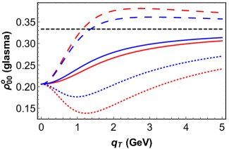
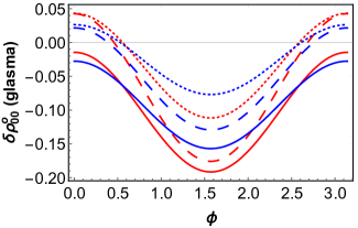
Figure 1: The left panel shows $\rho^{\rm o}_{00}$ with the transverse-momentum dependence, where the red and blue correspond to $y_{q}=0$ and $y_{q}=1$, respectively. The solid, dashed, and dotted curves are for $\phi=\pi/4$, $\phi=0$, and $\phi=\pi/2$. The black dashed line represents the base line for $\rho^{\rm o}_{00}=1/3$. The right panel shows $\delta\rho^{\rm o}_{00}=\rho^{\rm o}_{00}-1/3$ with the azimuthal angle dependence, where the red and blue correspond to $y_{q}=0$ and $y_{q}=1$, respectively. The solid, dashed, and dotted curves are for $q_{T}=1$, $q_{T}=2$, and $q_{T}=4$ GeV.

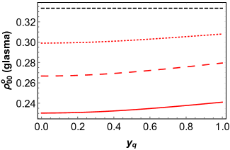
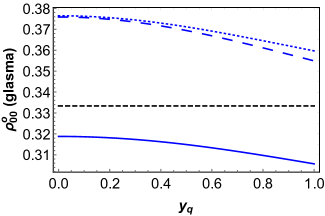
Figure 2: The left and right panels show $\rho^{\rm o}_{00}$ for $\phi$ mesons with the momentum-rapidity dependence for $\phi=\pi/4$ (red) and $\phi=0$ (blue), respectively. The solid, dashed, and dotted curves are for $q_{T}=1$, $q_{T}=2$, and $q_{T}=4$ GeV. The black dashed lines represent the base lines for $\rho^{\rm o}_{00}=1/3$.

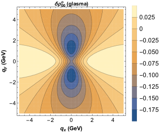
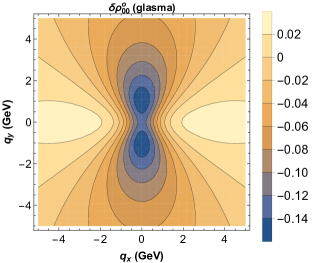
Figure 3: The contour plots for $\delta\rho^{\rm o}_{00}$ with respect to transverse momenta. The left and right panels correspond to $y_{q}=0$ and $y_{q}=1$, respectively.

On the left panel of Fig. 1, we plot $\rho^{\rm o}_{00}$ with $q_{T}$ dependence at fixed $y_{q}$ and $\phi$. Here $\rho^{\rm o}_{00}$ at $y_{q}=0$ and $y_{q}=1$ have similar behaviors with fixed $\phi$. In the case for $\phi=\pi/4$ ($q_{x}=q_{y}$), $\rho^{\rm o}_{00}<1/3$ and gradually approach $1/3$ at large $q_{T}$. However, with the maximum transverse momentum anisotropy at $\phi=0$ ($q_{y}=0$), it is found that $\rho^{\rm o}_{00}>1/3$ for sufficiently large $q_{T}$. Such an increase for $\rho^{\rm o}_{00}$ above $1/3$ could be anticipated from Eq. (72) with large $\gamma$, which yields

$$\rho^{\rm o}_{00}(q)\approx\frac{1}{3}\bigg{[}1+\frac{2}{3}\gamma C_{BE2}\big{(}3\hat{v}_{y}^{2}+\hat{v}_{z}^{2}-1\big{)}\bigg{]}=\frac{1}{3}\bigg{[}1+\frac{2}{3}\gamma C_{BE2}\big{(}2\hat{v}_{y}^{2}-\hat{v}_{x}^{2}\big{)}\bigg{]}$$ (86)

based on Eq. (85), where we have utilized $\hat{v}_{x}^{2}+\hat{v}_{y}^{2}+\hat{v}_{z}^{2}=1$ to acquire the second equality. It is clear to see that $\rho^{\rm o}_{00}>1/3$ when $\hat{v}_{x}^{2}>2\hat{v}_{y}^{2}$. On the contrary, when $\hat{v}_{x}^{2}<2\hat{v}_{y}^{2}$ as the cases for $\phi=\pi/4$ and $\phi=0$, $\rho^{\rm o}_{00}<1/3$ at large momenta. Note $\gamma\approx 3.74\cosh y_{q}$ for $q_{T}=4$ GeV. On the right panel of Fig. 1, we plot $\delta\rho^{\rm o}_{00}=\rho^{\rm o}_{00}-1/3$ with $\phi$ dependence at fixed $y_{q}$ and $q_{T}$. Consistently, for larger $q_{T}$, one finds that $\delta\rho^{\rm o}_{00}$ at $\phi=0$ and $\phi=\pi$ (both for $q_{y}=0$) could be positive. In light of Eq. (86), by taking $\hat{v}_{x}=\hat{v}_{T}\cos\phi$ and $\hat{v}_{y}=\hat{v}_{T}\sin\phi$ with $\hat{v}_{T}=\sqrt{\hat{v}_{x}^{2}+\hat{v}_{y}^{2}}$, it turns out that $\delta\rho^{\rm o}_{00}\sim-(2-3\cos^{2}\phi)$, which captures the qualitatively features of the results with large $q_{T}$.

In Fig. (2), we plot $\rho^{\rm o}_{00}$ with $y_{q}$ dependence at fixed $\phi$ and $q_{T}$. Generically, the $y_{q}$ dependence is relatively mild. Basically, $\rho^{\rm o}_{00}$ monotonically increases for $q_{x}=q_{y}$ and decreases for $q_{y}=0$. For large $q_{T}$, $\rho^{\rm o}_{00}$ could be larger than $1/3$ for $q_{y}=0$ as already indicated Fig. 1. We further show contour plots for $\delta\rho^{\rm o}_{00}$ with respect to transverse momenta in Fig. (3). In general, $\rho^{\rm o}_{00}<1/3$ in most of kinematic regions.

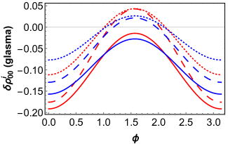
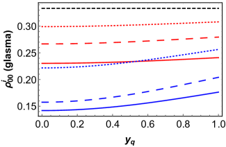
Figure 4: The left panel shows $\delta\rho^{\rm in}_{00}=\rho^{\rm o}_{00}-1/3$ with the azimuthal angle dependence with the same plot-style assignment in the right panel Fig. 1. The right panel shows $\rho^{\rm i}_{00}$ with $y_{q}$ dependence with the same plot-style assignment as Fig. 2.

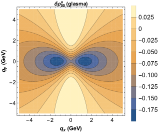
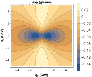
Figure 5: The contour plots for $\delta\rho^{\rm i}_{00}$ with respect to transverse momenta. The left and right panels correspond to $y_{q}=0$ and $y_{q}=1$, respectively.

Analogously, we may also numerically evaluate $\rho^{\rm i}_{00}$ for the in-plane spin alignment for $\phi$ mesons. Due to symmetry, the results for $\rho^{\rm i}_{00}$ with $q_{T}$ dependence at fixed $\phi$ and $y_{q}$ are the same as those shown in Fig. (1) by exchanging the results for $\phi=0$ and $\phi=\pi/2$. In Fig. 4, we further present $\delta\rho^{\rm i}_{00}$ with $\phi$ dependence and $\rho^{\rm i}_{00}$ with $y_{q}$ dependence, respectively. In particular, for the large-momentum limit, we simply need to exchange $\hat{v}_{x}$ and $\hat{v}_{y}$ in Eq. (86), which yields $\delta\rho^{\rm o}_{00}\sim-(2-3\sin^{2}\phi)$, and the qualitatively features of $\delta\rho^{\rm i}_{00}$ with $\phi$ dependence at large $q_{T}$ are understood. Also, $\rho^{\rm i}_{00}<1/3$ for either $\phi=\pi$ or $\phi=0$ is expected. The $y_{q}$ dependence is generically mild. The contour plots in Fig. 5 correspond to those in Fig. 3 with $90$-degree rotations.

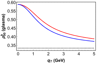
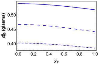
Figure 6: The left panel shows $\rho^{\rm b}_{00}$ with the transverse-momentum dependence and same plot-style assignment as the left panel of Fig. 1, while the curves from different $\phi$ coincide. The right panel shows $\rho^{\rm b}_{00}$ with the momentum-rapidity dependence and same plot-style assignment as Fig. 2. Similarly, all curves with different $\phi$ collapse to one.

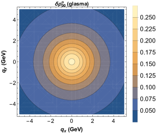
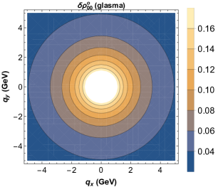
Figure 7: The contour plots for $\delta\rho^{\rm b}_{00}$ with respect to transverse momenta. The left and right panels correspond to $y_{q}=0$ and $y_{q}=1$, respectively.

Finally, we present the results for choosing the beam direction as the spin quantization axis. In such a case, sharper differences with respect to $\rho^{\rm o}_{00}$ and $\rho^{\rm i}_{00}$ are found. As manifested by the degeneracy of $C^{\rm b}_{x}$ and $C^{\rm b}_{y}$ in Eq. (IV.2), it is found that $\rho^{\rm b}_{00}$ is independent of $\phi$. In Fig. 6, we present $\rho^{\rm b}_{00}$ with $q_{T}$ dependence and $y_{q}$ dependence, respectively. Now, $\rho^{\rm b}_{00}$ is always greater than $1/3$ with mild $y_{q}$ dependence. As inferred from Eq. (79), $\rho^{\rm b}_{00}\rightarrow 1/3$ at large momenta given $|C_{BE2}|\gg|C_{BE1}|$. The contour plots of $\delta\rho^{\rm b}_{00}=\rho^{\rm b}_{00}-1/3$ are further shown in Fig. 7, which have rather distinct features with respect to $\delta\rho^{\rm o}_{00}$ and $\delta\rho^{\rm i}_{00}$. Here $\delta\rho^{\rm b}_{00}$ respects the transversely rotational symmetry and becomes more prominent in the center with small momenta.

V Spin alignment from color fields in QGP

In this section, we further investigate the spin alignment induced by chromo-electromagnetic fields in QGP or more precisely at the freeze-out hypersurface for chemical equilibrium in light of Eq. (17). One distinct feature here is that such color fields are expected to be isotropic in the lab frame. When considering the spin alignment led by non-dynamical spin polarization without intrinsic anisotropy, Eq. (III.3) for the out-of-plane spin alignment has to be slightly modified as

$$\rho_{00}(q)=\frac{1-\big{[}\big{(}\tilde{C}_{B1}+\tilde{C}_{B2}\big{)}\chi^{yy}_{B}+\tilde{C}_{B1}(\chi^{xx}_{B}+\chi^{zz}_{B}\big{)}+\big{(}\tilde{C}_{E1}+\tilde{C}_{E2}\big{)}\chi^{yy}_{E}+\tilde{C}_{E1}(\chi^{xx}_{E}+\chi^{zz}_{E}\big{)}\big{]}}{3-\big{[}\big{(}3\tilde{C}_{B1}+\tilde{C}_{B2}\big{)}\chi_{B}+\big{(}3\tilde{C}_{E1}+\tilde{C}_{E2}\big{)}\chi_{E}\big{]}},$$ (87)

where

$$\tilde{C}_{B1,2}=C_{B1,2}\frac{\hbar^{2}g^{2}C_{AB}}{\pi^{2}m_{q}m_{\bar{q}}C_{V}N_{c}^{2}},\quad\tilde{C}_{E1,2}=C_{E1,2}\frac{\hbar^{2}g^{2}C_{AE}}{\pi^{2}m_{q}m_{\bar{q}}C_{V}N_{c}^{2}},$$ (88)

and

$$C_{AB} = \frac{\big{(}\partial_{\epsilon_{q\tilde{k}}}f_{qV}(\epsilon_{q\tilde{k}},t_{\rm eq})\big{)}\big{(}\partial_{\epsilon_{\bar{q}\tilde{k}}}f_{\bar{q}V}(\epsilon_{\bar{q}\tilde{k}},t_{\rm eq})\big{)}}{16\epsilon_{q\tilde{k}}\epsilon_{\bar{q}\tilde{k}}},$$ (89)

$$C_{AE} = \frac{1}{64\epsilon_{q\tilde{k}}\epsilon_{\bar{q}\tilde{k}}}\bigg{(}\big{(}\partial_{\epsilon_{q\tilde{k}}}f_{qV}(\epsilon_{q\tilde{k}},t_{\rm eq})\big{)}+\frac{f_{qV}(\epsilon_{q\tilde{k}},t_{\rm eq})}{\epsilon_{q\tilde{k}}}\bigg{)}\bigg{(}\big{(}\partial_{\epsilon_{\bar{q}\tilde{k}}}f_{\bar{q}V}(\epsilon_{\bar{q}\tilde{k}},t_{\rm eq})+\frac{f_{\bar{q}V}(\epsilon_{\bar{q}\tilde{k}},t_{\rm eq})}{\epsilon_{\bar{q}\tilde{k}}}\bigg{)}.$$ (90)

Here the correlators of color fields are presumed to take the form

$$\chi_{B}^{ij}=\big{\langle}B^{ai}(t_{\rm eq},\bm{x})B^{aj}(t_{\rm eq},\bm{x})\big{\rangle}\delta^{ij},\quad\chi_{E}^{ij}=\big{\langle}E^{ai}(t_{\rm eq},\bm{x})E^{aj}(t_{\rm eq},\bm{x})\big{\rangle}\delta^{ij},$$ (91)

where we consider equal-spacetime correlators or simply the constant color-field square at the freeze-out hypersurface for $x_{0}=t_{\rm eq}$. From Eqs. (IV.2) and (59), we have

$$\chi_{B}^{xx}(q) = \gamma^{2}\big{(}\chi_{0B}^{xx}+v_{y}^{2}\chi_{0E}^{zz}+v_{z}^{2}\chi_{0E}^{yy}\big{)}-2\gamma(\gamma-1)\chi_{0B}^{xx}\hat{v}_{x}^{2}+(\gamma-1)^{2}\hat{v}_{x}^{2}\chi_{0B},$$

$$\chi_{B}^{yy}(q) = \gamma^{2}\big{(}\chi_{0B}^{yy}+v_{x}^{2}\chi_{0E}^{zz}+v_{z}^{2}\chi_{0E}^{xx}\big{)}-2\gamma(\gamma-1)\chi_{0B}^{yy}\hat{v}_{x}^{2}+(\gamma-1)^{2}\hat{v}_{y}^{2}\chi_{0B},$$

$$\chi_{B}^{zz}(q) = \gamma^{2}\big{(}\chi_{0B}^{zz}+v_{y}^{2}\chi_{0E}^{xx}+v_{x}^{2}\chi_{0E}^{yy}\big{)}-2\gamma(\gamma-1)\chi_{0B}^{zz}\hat{v}_{z}^{2}+(\gamma-1)^{2}\hat{v}_{z}^{2}\chi_{0B},$$ (92)

and

$$\chi_{E}^{xx}(q) = \gamma^{2}\big{(}\chi_{0E}^{xx}+v_{y}^{2}\chi_{0B}^{zz}+v_{z}^{2}\chi_{0B}^{yy}\big{)}-2\gamma(\gamma-1)\chi_{0E}^{xx}\hat{v}_{x}^{2}+(\gamma-1)^{2}\hat{v}_{x}^{2}\chi_{0E},$$

$$\chi_{E}^{yy}(q) = \gamma^{2}\big{(}\chi_{0E}^{yy}+v_{x}^{2}\chi_{0B}^{zz}+v_{z}^{2}\chi_{0B}^{xx}\big{)}-2\gamma(\gamma-1)\chi_{0E}^{yy}\hat{v}_{x}^{2}+(\gamma-1)^{2}\hat{v}_{y}^{2}\chi_{0E},$$

$$\chi_{E}^{zz}(q) = \gamma^{2}\big{(}\chi_{0E}^{zz}+v_{y}^{2}\chi_{0B}^{xx}+v_{x}^{2}\chi_{0B}^{yy}\big{)}-2\gamma(\gamma-1)\chi_{0E}^{zz}\hat{v}_{z}^{2}+(\gamma-1)^{2}\hat{v}_{z}^{2}\chi_{0E},$$ (93)

where $\chi_{0B,E}^{ij}=\chi_{B,E}^{ij}(q=0)$ and $\chi_{0B,E}=\chi_{0B,E}^{xx}+\chi_{0B,E}^{yy}+\chi_{0B,E}^{zz}$. When further postulating $\chi_{0B}^{ii}=\chi_{0E}^{ii}=\chi_{0}$ such that the isotropic chromo-electric correlator and the chromo-magnetic one are further degenerate, it is found

$$\chi_{B}^{xx}(q) = \chi_{E}^{xx}(q)=\big{(}2\gamma^{2}-1+4(1-\gamma)\hat{v}_{x}^{2})\big{)}\chi_{0},$$

$$\chi_{B}^{yy}(q) = \chi_{E}^{yy}(q)=\big{(}2\gamma^{2}-1+4(1-\gamma)\hat{v}_{y}^{2})\big{)}\chi_{0},$$

$$\chi_{B}^{zz}(q) = \chi_{E}^{zz}(q)=\big{(}2\gamma^{2}-1+4(1-\gamma)\hat{v}_{z}^{2})\big{)}\chi_{0}.$$ (94)

For the out-of-plane spin alignment, it turns out that

$$\rho^{\rm o}_{00}(q) = \frac{1-\big{[}\big{(}\tilde{C}_{BE1}+\tilde{C}_{BE2}\big{)}\chi^{yy}_{B}+\tilde{C}_{BE1}(\chi^{xx}_{B}+\chi^{zz}_{B}\big{)}\big{]}}{3-\big{(}3\tilde{C}_{BE1}+\tilde{C}_{BE2}\big{)}\chi_{B}}$$ (95)

$$= \frac{1-\big{(}3\tilde{C}_{BE1}+\tilde{C}_{BE2}\big{)}(2\gamma^{2}-1)-4(1-\gamma)(\tilde{C}_{BE1}+\tilde{C}_{BE2}\hat{v}_{y}^{2})}{3-\big{(}3\tilde{C}_{BE1}+\tilde{C}_{BE2}\big{)}(6\gamma^{2}-4\gamma+1)},$$

where $\tilde{C}_{BE1,2}=(\tilde{C}_{B1,2}+\tilde{C}_{E1,2})\chi_{0}$. Similarly, it is found

$$\rho^{\rm i}_{00}(q) = \frac{1-\big{(}3\tilde{C}_{BE1}+\tilde{C}_{BE2}\big{)}(2\gamma^{2}-1)-4(1-\gamma)(\tilde{C}_{BE1}+\tilde{C}_{BE2}\hat{v}_{x}^{2})}{3-\big{(}3\tilde{C}_{BE1}+\tilde{C}_{BE2}\big{)}(6\gamma^{2}-4\gamma+1)}$$ (96)

for the out-of-plane spin alignment and

$$\rho^{\rm b}_{00}(q) = \frac{1-\big{(}3\tilde{C}_{BE1}+\tilde{C}_{BE2}\big{)}(2\gamma^{2}-1)-4(1-\gamma)(\tilde{C}_{BE1}+\tilde{C}_{BE2}\hat{v}_{z}^{2})}{3-\big{(}3\tilde{C}_{BE1}+\tilde{C}_{BE2}\big{)}(6\gamma^{2}-4\gamma+1)}$$ (97)

for the longitudinal spin alignment.

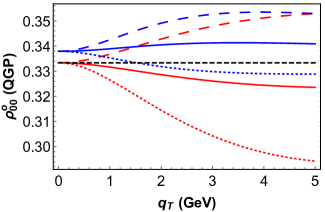
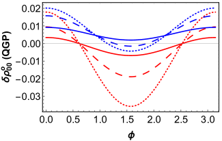
Figure 8: Same plot setting as Fig. 1 for the out-of-plane spin alignment from QGP.

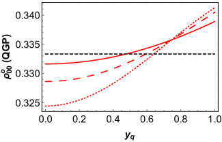
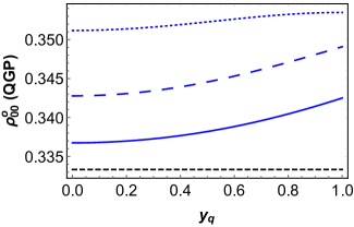
Figure 9: Same plot setting as Fig. 2 for the out-of-plane spin alignment from QGP.

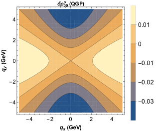
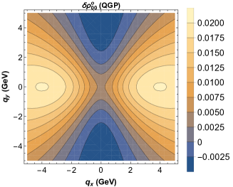
Figure 10: Same plot setting as Fig. 3 for the out-of-plane spin alignment from QGP.

Subsequently, we may adopt the same numerical parameters as in the previous section to evaluate spin alignment with different spin quantization axes. However, unlike the case for glasma fields, here we simply approximate $\chi_{0}=g^{2}T_{\rm eq}^{4}$ as the strength of color-field correlators in QGP at the freeze-out hypersurface for simplicity and take $\alpha_{s}=g^{2}/(4\pi)=1/3$. Recall that the primary purpose in this section is to analyze the qualitative features instead of making precise predictions quantitatively. In Fig. 8, we plot $\rho^{\rm o}_{00}$ with $q_{T}$ dependence and $\delta\rho^{o}_{00}$ with $\phi$ dependence as a comparison with those from glasma fields in Fig. 1. Unlike the results from glasma, now the spin alignment is induced by finite momenta as observed from the red curves in the left panel of Fig. 8, where $\rho^{\rm o}_{00}=1/3$ when $q_{T}=0$ and $y_{q}=0$. Given Eq. (85) and correspondingly $\tilde{C}_{BE2}<0$ and $|\tilde{C}_{BE2}|\gg\tilde{C}_{BE1}>0$ for $\phi$ mesons, we may approximate Eq. (95) as

$$\rho^{\rm o}_{00}(q) \approx \frac{1-\tilde{C}_{BE2}\big{(}2\gamma^{2}-1+4(1-\gamma)\hat{v}_{y}^{2}\big{)}}{3-\tilde{C}_{BE2}(6\gamma^{2}-4\gamma+1)},$$ (98)

which further reduces to

$$\rho^{\rm o}_{00}(q)\approx\frac{1}{3}\Big{[}1+4\tilde{C}_{BE2}(\gamma-1)\Big{(}\hat{v}_{y}^{2}-\frac{1}{3}\Big{)}\Big{]}$$ (99)

for weak correlations. According to Eq. (99), one immediately finds $\rho^{\rm o}_{00}>1/3$ when $\hat{v}_{y}^{2}<1/3$ especially at the large-momentum limit. The $\phi$ dependence of $\rho^{\rm o}_{00}$ is then shown on the right panel of Fig. 8. Nevertheless, from Eq. (99) with larger $\gamma$, we also obtains $\delta\rho^{\rm o}_{00}\sim-(2-3\cos^{2}\phi)$ as the same qualitative feature in the case with glasma fields. We also plot $\rho^{\rm o}_{00}$ with the momentum-rapidity dependence in Fig. 9. One observes the monotonic increase with respect to $y_{q}$ especially for $\phi=\pi/4$ shown on the left panel. Finally, the contour plots with transverse-momentum dependence are shown in Fig. 10, where now $\delta\rho^{\rm o}_{00}$ is more prominent away from the center with small momenta, which is also anticipated since the spin alignment is now triggered by momentum anisotropy. Overall, the out-of-plane spin alignment from the isotropic color fields in QGP is qualitatively consistent with the one from fluctuating meson fields in Refs. [54, 61]. When comparing the results here with those from the glasma effect, one may particularly focus on the $q_{T}$ dependence and also the detailed transverse-momenta dependence shown in the contour plots for $\rho^{\rm o}_{00}$, where the distinct qualitative features are found from our analyses.

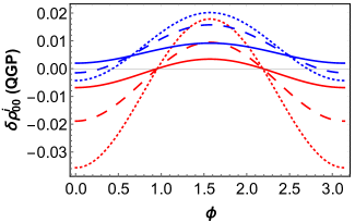
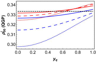
Figure 11: Same plot setting as Fig. 4 for the in-plane spin alignment from QGP.

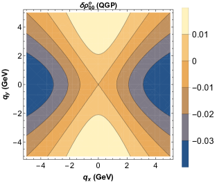
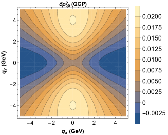
Figure 12: Same plot setting as Fig. 5 for the in-plane spin alignment from QGP.

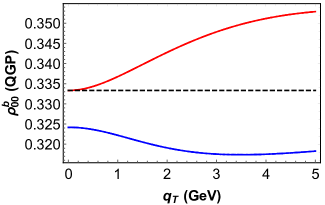
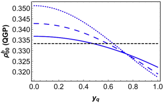
Figure 13: Same plot setting as Fig. 6 for the longitudinal spin alignment from QGP.

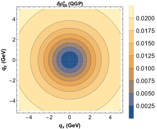
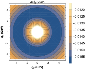
Figure 14: Same plot setting as Fig. 14 for the longitudinal spin alignment from QGP.

One may analogously evaluate $\rho^{\rm i}_{00}$, for which we present some of numerical results in Fig. 11 and Fig. 12. Several features can be explained by symmetry as the case for the glasma effect. Finally, we evaluate the longitudinal spin alignment for isotropic color fields from QGP, for which there exists no $\phi$ dependence by symmetry. On the left panel of Fig. 13, the $q_{T}$ dependence of $\rho^{\rm b}_{00}$ is shown, for which the qualitative behaviors may be captured by the approximated form in Eq. (99) by replacing $\hat{v}_{y}$ with $\hat{v}_{z}$. Since $\hat{v}_{z}=0$ for $y_{q}=0$, it is clear to see that $\delta\rho^{\rm b}_{00}$ monotonically increases from zero stemming from the $\gamma-1$ prefactor. For $y_{q}=1$ and $\hat{v}_{z}^{2}>1/3$, $\delta\rho^{\rm b}_{00}$ is negative at $q_{T}=0$, while the variation with $q_{T}$ is more subtle since $\hat{v}_{z}$ also depends on $q_{T}$. The $y_{q}$ dependence at fixed $q_{T}$ is also shown on the right panel of Fig. 13. Here $\delta\rho^{\rm b}_{00}$ can change from positive to negative when $y_{q}$ changes from $\hat{v}_{z}^{2}<1/3$ to $\hat{v}_{z}^{2}>1/3$. Eventually, the contour plots with transverse-momenta dependence are shown in Fig. 14. As already discussed, the sign of $\delta\rho^{\rm b}_{00}$ depends on $y_{q}$, whereas $\delta\rho^{\rm b}_{00}$ is more prominent away from the center with small momenta as a generic feature from isotropic color fields as opposed to the case for anisotropic color fields from the glasma. It is evident that the longitudinal spin alignment shows drastically qualitative difference between the color fields from QGP and glasma.

VI Conclusions and outlook

In this paper, we study the momentum dependence of transverse and longitudinal spin alignment for $\phi$ mesons induced by the color fields from both the glasma phase and QGP in the quark coalescence scenarios. For the spin alignment from the glasma effect, it is found that large transverse-momentum anisotropy could overcome the effect from intrinsic anisotropy led by the longitudinally dominant glasma fields at large transverse momenta, which results in the sign flipping of $\delta\rho_{00}$ as the deviation from the baseline $\rho_{00}=1/3$ at intermediate momenta for transverse spin alignment and especially the out-of-plane case. Moreover, for longitudinal spin alignment from glasma fields, the azimuthal-angle dependence vanishes and its transverse-momentum dependence has rather distinct patterns with respect to the cases for transverse spin alignment. For the transverse spin alignment induced by isotropic color fields in the QGP, we find similar patterns qualitatively consistent with that by fluctuating vector-meson fields in the previous studies, while several differences from the glasma effect are more manifested with momentum dependence. On the other hand, the qualitative differences between the glasma effect and the color fields in QGP are even more robust for longitudinal spin alignment. In the following, we further discuss some potential issues about our approach and future directions.

For more straightforward comparisons with present and future experimental observations, $\rho_{00}$ weighted by the particle momentum spectra is needed. But qualitatively, the azimuthal-angle dependence for $0\leq\phi\leq\pi/4$ should be correlated with the elliptic flow or indirectly the centrality dependence from more peripheral $(\phi\rightarrow 0)$ to more central $(\phi\rightarrow\pi/4)$ collisions. Also, when integrating over $q_{T}$, one may expect more dominant contributions from the low-$q_{T}$ region due to the weighting. Nevertheless, before conducting such more refined studies in phenomenology, we may have to first address several fundamental limitations and insufficiency regarding our theoretical approach as will be partly elaborated below.

Regarding the flavor dependence, although we have lifted the equal-mass condition for the collision kernel responsible for the quark coalescence, we have not applied the formalism to vector mesons composed of quarks and antiquarks with different flavors. For $K^{*0}$, due to the short lifetime, they may further decay and regenerate in the hadronic phase [92, 93], for which the spin correlation built up in even the QGP phase could be modified. On the other hand, it may be questionable for the validity of QKT for light quarks with quasi-particle approximation in the strongly coupled QGP. Assuming the spin correlation can be induced by glasma fields in the pre-equilibrium phase, it is curious and indispensable to further investigate how such a microscopic quantity could be incorporated in a dissipative effective theory such as the viscous hydrodynamics to address the spin relaxation in a non-perturbative manner in QGP.

In fact, the weak-field approximation adopted to perturbatively solve the QKT could also be invalid given the glasma fields are actually non-perturbative. For example, a more thorough analysis for the competition between the color-octet and color-singlet contributions has been previously presented in Ref. [60]. Generically, the QKT should be more applicable to heavy flavor, for which the scale separation is achievable. The suitable candidates such as the spin alignment of $J/\psi$ has been recently measured [42]. However, the quarkonia are more deeply bounded than light mesons. They undergo the screening, dynamical dissociation, and even recombination in the QGP. A recent study upon the construction of polarization-dependent QKT for vector quarkonia from open quantum systems and effective field theories was done in Ref. [94], from which one may also investigate the spin alignment triggered by color fields in the QGP phase in a non-perturbative fashion. Nevertheless, how to incorporate the early-time spin correlation before the QGP phase in such a framework is unknown and the glasma effect for spin alignment also highly depends on the initial quark and antiquark distributions. In conclusion, tremendous efforts are still needed to understand the spin alignment of vector mesons with the underlying mechanisms in connection to the QCD interaction and microscopic properties of QGP or even the pre-equilibrium phase in high-energy nuclear collisions.

Appendix A Detailed calculations for quark coalescence

Eqs. (27) and (LABEL:eq:useful_rel_2) yield

$$-\frac{2|k\cdot\epsilon(\lambda,{\bm{q}})|^{2}}{N_{m}}\rightarrow-\frac{2|\bm{k}|^{2}\bar{z}^{2}}{N_{m}},$$ (100)

$$\mathcal{A}_{q}(\bm{p},x)\cdot\mathcal{A}_{\bar{q}}(\bm{p}^{\prime},x) \rightarrow \eta^{ij}\mathcal{A}_{qi}^{(0)}\mathcal{A}_{\bar{q}j}^{(0)}-\frac{|\bm{k}|^{2}}{\epsilon_{q\bm{k}}\epsilon_{\bar{q}\bm{k}}}\Big{[}\bar{z}^{2}\epsilon^{i}_{\lambda}\epsilon^{j}_{\lambda}-\frac{(1-\bar{z}^{2})}{2}\hat{\Theta}^{ij}_{\lambda}\Big{]}\mathcal{A}_{qi}^{(0)}\mathcal{A}_{\bar{q}j}^{(0)}$$ (101)

$$-|\bm{k}|^{2}\Big{[}\bar{z}^{2}\epsilon^{i}_{\lambda}\epsilon^{j}_{\lambda}-\frac{(1-\bar{z}^{2})}{2}\hat{\Theta}^{ij}_{\lambda}\Big{]}\mathcal{A}_{qil}^{(1)}\mathcal{A}_{\bar{q}j}^{(1)l}$$

$$= \eta^{ij}\mathcal{A}_{qi}^{(0)}\mathcal{A}_{\bar{q}j}^{(0)}\left[1+\frac{|\bm{k}|^{2}(1-\bar{z}^{2})}{2\epsilon_{q\bm{k}}\epsilon_{\bar{q}\bm{k}}}\right]+\frac{|\bm{k}|^{2}(1-3\bar{z}^{2})}{2\epsilon_{q\bm{k}}\epsilon_{\bar{q}\bm{k}}}\epsilon^{i}_{\lambda}\epsilon^{j}_{\lambda}\mathcal{A}_{qi}^{(0)}\mathcal{A}_{\bar{q}j}^{(0)}$$

$$+\frac{|\bm{k}|^{2}}{2}\big{[}(1-\bar{z}^{2})\mathcal{A}_{qij}^{(1)}\mathcal{A}_{\bar{q}}^{(1)ij}+(1-3\bar{z}^{2})\epsilon^{i}_{\lambda}\epsilon^{j}_{\lambda}\mathcal{A}_{qil}^{(1)}\mathcal{A}_{\bar{q}j}^{(1)l}\big{]},$$

$$-\frac{2|k\cdot\epsilon(\lambda,{\bm{q}})|^{2}}{N_{m}}\mathcal{A}_{q}(\bm{p},x)\cdot\mathcal{A}_{\bar{q}}(\bm{p}^{\prime},x)$$

$$\rightarrow-\frac{2|\bm{k}|^{2}\bar{z}^{2}}{N_{m}}\eta^{ij}\mathcal{A}_{qi}^{(0)}\mathcal{A}_{\bar{q}j}^{(0)}+\frac{2|\bm{k}|^{4}}{N_{m}\epsilon_{q\bm{k}}\epsilon_{\bar{q}\bm{k}}}\hat{\Theta}^{ijln}_{\lambda}\epsilon_{\lambda i}\epsilon_{\lambda j}\mathcal{A}_{ql}^{(0)}\mathcal{A}_{qn}^{(0)}+\frac{2|\bm{k}|^{4}}{N_{m}}\hat{\Theta}^{ijln}_{\lambda}\epsilon_{\lambda i}\epsilon_{\lambda j}\mathcal{A}_{qlk}^{(1)}\mathcal{A}_{\bar{q}n}^{(1)k}$$

$$=-\frac{2|\bm{k}|^{2}}{N_{m}}\bigg{[}\bar{z}^{2}\eta^{ij}\mathcal{A}_{qi}^{(0)}\mathcal{A}_{\bar{q}j}^{(0)}\left(1+\frac{|\bm{k}|^{2}(1-\bar{z}^{2})}{2\epsilon_{q\bm{k}}\epsilon_{\bar{q}\bm{k}}}\right)-\frac{|\bm{k}|^{2}\bar{z}^{2}(1-7\bar{z}^{2})}{2\epsilon_{q\bm{k}}\epsilon_{\bar{q}\bm{k}}}\epsilon^{i}_{\lambda}\epsilon^{j}_{\lambda}\mathcal{A}_{qi}^{(0)}\mathcal{A}_{\bar{q}j}^{(0)}$$

$$\quad+\frac{|\bm{k}|^{2}\bar{z}^{2}}{2}\big{(}(1-\bar{z}^{2})\mathcal{A}_{qij}^{(1)}\mathcal{A}_{\bar{q}}^{(1)ij}+(1-7\bar{z}^{2})\epsilon^{i}_{\lambda}\epsilon^{j}_{\lambda}\mathcal{A}_{qil}^{(1)}\mathcal{A}_{\bar{q}j}^{(1)l}\big{)}\bigg{]},$$ (102)

$$2{\rm Re}\Big{(}\epsilon(\lambda,{\bm{q}})\cdot\mathcal{A}_{q}(\bm{p},x)\epsilon^{*}(\lambda,{\bm{q}})\cdot\mathcal{A}_{\bar{q}}(\bm{p}^{\prime},x)\Big{)}$$

$$\rightarrow 2\epsilon_{\lambda}\cdot\mathcal{A}_{q}^{(0)}\epsilon_{\lambda}\cdot\mathcal{A}_{\bar{q}}^{(0)}-2|\bm{k}|^{2}\Big{[}\bar{z}^{2}\epsilon^{i}_{\lambda}\epsilon^{j}_{\lambda}-\frac{(1-\bar{z}^{2})}{2}\hat{\Theta}^{ij}_{\lambda}\Big{]}\mathcal{A}_{qik}^{(1)}\mathcal{A}_{\bar{q}jl}^{(1)}\epsilon^{k}_{\lambda}\epsilon^{l}_{\lambda}$$

$$=2\epsilon_{\lambda}\cdot\mathcal{A}_{q}^{(0)}\epsilon_{\lambda}\cdot\mathcal{A}_{\bar{q}}^{(0)}+|\bm{k}|^{2}(1-\bar{z}^{2})\epsilon^{i}_{\lambda}\epsilon^{j}_{\lambda}\mathcal{A}_{qil}^{(1)}\mathcal{A}_{\bar{q}j}^{(1)l},$$ (103)

$$2k\cdot\mathcal{A}_{q}(\bm{p})k\cdot\mathcal{A}_{\bar{q}}(\bm{p}^{\prime}) \rightarrow 2|\bm{k}|^{2}\left(1-\frac{k_{0}^{2}}{\epsilon_{q\bm{k}}\epsilon_{\bar{q}\bm{k}}}\right)\Big{[}\bar{z}^{2}\epsilon^{i}_{\lambda}\epsilon^{j}_{\lambda}-\frac{(1-\bar{z}^{2})}{2}\hat{\Theta}^{ij}_{\lambda}\Big{]}\mathcal{A}_{qi}^{(0)}\mathcal{A}_{\bar{q}j}^{(0)},$$ (104)

$$= -|\bm{k}|^{2}\left(1-\frac{k_{0}^{2}}{\epsilon_{q\bm{k}}\epsilon_{\bar{q}\bm{k}}}\right)\big{[}(1-3\bar{z}^{2})\big{(}\epsilon_{\lambda}\cdot\mathcal{A}_{q}^{(0)}\epsilon_{\lambda}\cdot\mathcal{A}_{\bar{q}}^{(0)}\big{)}$$

$$+(1-\bar{z}^{2})\eta^{ij}\mathcal{A}_{qi}^{(0)}\mathcal{A}_{\bar{q}j}^{(0)}\big{]},$$

$${\rm Re}\big{(}k\cdot\epsilon(\lambda,{\bm{q}})\mathcal{A}_{q}(\bm{p})\cdot\epsilon^{*}(\lambda,{\bm{q}})\big{)}k\cdot\mathcal{A}_{\bar{q}}(\bm{p}^{\prime}) \rightarrow -\bar{z}^{2}|\bm{k}|^{2}\epsilon_{\lambda}\cdot\mathcal{A}_{q}^{(0)}\epsilon_{\lambda}\cdot\mathcal{A}_{\bar{q}}^{(0)},$$ (105)

and

$${\rm Re}\big{(}k\cdot\epsilon(\lambda,{\bm{q}})\mathcal{A}_{\bar{q}}(\bm{p}^{\prime})\cdot\epsilon^{*}(\lambda,{\bm{q}})\big{)}k\cdot\mathcal{A}_{q}(\bm{p}) \rightarrow -\bar{z}^{2}|\bm{k}|^{2}\epsilon_{\lambda}\cdot\mathcal{A}_{q}^{(0)}\epsilon_{\lambda}\cdot\mathcal{A}_{\bar{q}}^{(0)},$$ (106)

where $\epsilon_{q/\bar{q}\bm{k}}\equiv\sqrt{|\bm{k}|^{2}+m^{2}_{q/\bar{q}}}$ is the abbreviation of $\epsilon_{q/\bar{q}}(\bm{k})$. For a complex $\epsilon^{\mu}_{\lambda}$, it is expected that one could simply replace $\big{(}\epsilon_{\lambda}\cdot\mathcal{A}_{q}(\bm{q}/2)\epsilon_{\lambda}\cdot\mathcal{A}_{\bar{q}}(\bm{q}/2)\big{)}$ by ${\rm Re}\big{(}\epsilon_{\lambda}\cdot\mathcal{A}_{q}(\bm{q}/2)\epsilon^{*}_{\lambda}\cdot\mathcal{A}_{\bar{q}}(\bm{q}/2)\big{)}$ and $\epsilon_{\lambda i}\mathcal{A}_{qjm}^{(1)}\epsilon^{m}_{\lambda}\mathcal{A}_{\bar{q}nl}^{(1)}$ by ${\rm Re}\big{(}\epsilon_{\lambda i}\mathcal{A}_{qjm}^{(1)}\epsilon^{*m}_{\lambda}\mathcal{A}_{\bar{q}nl}^{(1)}\big{)}$ (and similarly $\epsilon_{\lambda i}\mathcal{A}_{\bar{q}jm}^{(1)}\epsilon^{m}_{\lambda}\mathcal{A}_{qnl}^{(1)}$) in the final result.

Now, by using Eqs. (101)-(106), we find

$$\mathcal{C}_{{\rm col},\lambda}(q)$$

$$=N_{m}\int\frac{d^{3}k}{(2\pi)^{3}}\frac{\big{(}M^{4}-(m_{q}^{2}-m_{\bar{q}}^{2})^{2}\big{)}\delta\big{(}|\bm{k}|-\tilde{k}\big{)}}{8M^{3}\tilde{k}}\Bigg{\{}\frac{N_{c}^{2}f_{Vq}(\epsilon_{q\bm{k}},x_{0})f_{V\bar{q}}(\epsilon_{\bar{q}\tilde{k}},x_{0})}{\epsilon_{q\tilde{k}}\epsilon_{\bar{q}\tilde{k}}}\big{(}1-2C_{m}\bar{z}^{2}\big{)}$$

$$\quad-\frac{2}{m_{q}m_{\bar{q}}}\Bigg{[}\bigg{(}\big{(}1-2C_{m}\big{)}+\frac{\tilde{k}^{2}}{2\epsilon_{q\tilde{k}}\epsilon_{\bar{q}\tilde{k}}}\big{(}1-2C_{m}\bar{z}^{2}\big{)}+\frac{2k_{0}^{2}(1-\bar{z}^{2})}{\epsilon_{q\tilde{k}}\epsilon_{\bar{q}\tilde{k}}}\bigg{)}\eta^{ij}\big{\langle}\mathcal{A}_{qi}^{a(0)}\mathcal{A}_{\bar{q}j}^{a(0)}\big{\rangle}$$

$$\quad+\bigg{(}2\big{(}1-C_{m}(1+\bar{z}^{2})\big{)}+\frac{\tilde{k}^{2}}{2\epsilon_{q\tilde{k}}\epsilon_{\bar{q}\tilde{k}}}\big{(}1-3\bar{z}^{2}+2C_{m}\bar{z}^{2}(1-7\bar{z}^{2})\big{)}+\frac{2k_{0}^{2}(1-3\bar{z}^{2})}{\epsilon_{q\tilde{k}}\epsilon_{\bar{q}\tilde{k}}}\bigg{)}$$

$$\quad\times{\rm Re}\Big{(}\big{\langle}\epsilon_{\lambda}\cdot\mathcal{A}_{q}^{a(0)}\epsilon^{*}_{\lambda}\cdot\mathcal{A}_{\bar{q}}^{a(0)}\big{\rangle}\Big{)}+\frac{|\bm{k}|^{2}}{2}(1-\bar{z}^{2})(1-2C_{m}\bar{z}^{2})\big{\langle}\mathcal{A}_{qij}^{a(1)}\mathcal{A}_{\bar{q}}^{a(1)ij}\big{\rangle}$$

$$\quad+\frac{|\bm{k}|^{2}}{2}\big{(}(2-5\bar{z}^{2})-2C_{m}\bar{z}^{2}(1-7\bar{z}^{2})\big{)}{\rm Re}\Big{(}\big{\langle}\epsilon^{i}_{\lambda}\epsilon^{*j}_{\lambda}\mathcal{A}_{qil}^{a(1)}\mathcal{A}_{\bar{q}j}^{a(1)l}\big{\rangle}\Big{)}\Bigg{]}\Bigg{\}},$$ (107)

where

$$\epsilon_{q/\bar{q}\tilde{k}}\equiv\sqrt{\tilde{k}^{2}+m^{2}_{q/\bar{q}}}=\frac{1}{2M}\big{[}(m_{q/\bar{q}}^{2}-m_{\bar{q}/q}^{2})+M^{2}\big{]}$$ (108)

and

$$C_{m}\equiv\frac{\tilde{k}^{2}}{N_{m}}=\frac{1}{2}\left(1-\frac{(m_{q}-m_{\bar{q}})^{2}}{M^{2}}\right).$$ (109)

Here we have presumably evaluated the correlation of Wigner functions for the quark and antiquark before conducting the $k$ integral and written down a generic expression for both real and complex $\epsilon_{\lambda}$. After integrating over $\bar{z}$, we arrive at Eq. (29)

References

- Liang and Wang [2005a] Z.-T. Liang and X.-N. Wang, Globally polarized quark-gluon plasma in non-central A+A collisions, Phys. Rev. Lett. 94, 102301 (2005a), [Erratum: Phys. Rev. Lett.96,039901(2006)], arXiv:nucl-th/0410079 [nucl-th] .
- Liang and Wang [2005b] Z.-T. Liang and X.-N. Wang, Spin alignment of vector mesons in non-central A+A collisions, Phys. Lett. B 629, 20 (2005b), arXiv:nucl-th/0411101 .
- Voloshin [2004] S. A. Voloshin, Polarized secondary particles in unpolarized high energy hadron-hadron collisions?, (2004), arXiv:nucl-th/0410089 [nucl-th] .
- Adamczyk et al. [2017] L. Adamczyk et al. (STAR), Global hyperon polarization in nuclear collisions: evidence for the most vortical fluid, Nature 548, 62 (2017), arXiv:1701.06657 [nucl-ex] .
- Adam et al. [2019] J. Adam et al. (STAR), Polarization of () hyperons along the beam direction in Au+Au collisions at = 200 GeV, Phys. Rev. Lett. 123, 132301 (2019), arXiv:1905.11917 [nucl-ex] .
- Acharya et al. [2020a] S. Acharya et al. (ALICE), Global polarization of hyperons in Pb-Pb collisions at = 2.76 and 5.02 TeV, Phys. Rev. C 101, 044611 (2020a), arXiv:1909.01281 [nucl-ex] .
- Kornas [2020] F. J. Kornas (HADES), Polarization in Au+Au Collisions at Measured with HADES, Springer Proc. Phys. 250, 435 (2020).
- Becattini et al. [2013] F. Becattini, V. Chandra, L. Del Zanna, and E. Grossi, Relativistic distribution function for particles with spin at local thermodynamical equilibrium, Annals Phys. 338, 32 (2013), arXiv:1303.3431 [nucl-th] .
- Becattini et al. [2017] F. Becattini, I. Karpenko, M. Lisa, I. Upsal, and S. Voloshin, Global hyperon polarization at local thermodynamic equilibrium with vorticity, magnetic field and feed-down, Phys. Rev. C95, 054902 (2017), arXiv:1610.02506 [nucl-th] .
- Karpenko and Becattini [2017] I. Karpenko and F. Becattini, Study of polarization in relativistic nuclear collisions at –200 GeV, Eur. Phys. J. C 77, 213 (2017), arXiv:1610.04717 [nucl-th] .
- Becattini and Karpenko [2018] F. Becattini and I. Karpenko, Collective Longitudinal Polarization in Relativistic Heavy-Ion Collisions at Very High Energy, Phys. Rev. Lett. 120, 012302 (2018), arXiv:1707.07984 [nucl-th] .
- Fang et al. [2016] R.-h. Fang, L.-g. Pang, Q. Wang, and X.-n. Wang, Polarization of massive fermions in a vortical fluid, Phys. Rev. C 94, 024904 (2016), arXiv:1604.04036 [nucl-th] .
- Xia et al. [2018] X.-L. Xia, H. Li, Z.-B. Tang, and Q. Wang, Probing vorticity structure in heavy-ion collisions by local polarization, Phys. Rev. C 98, 024905 (2018), arXiv:1803.00867 [nucl-th] .
- Fu et al. [2021a] B. Fu, K. Xu, X.-G. Huang, and H. Song, Hydrodynamic study of hyperon spin polarization in relativistic heavy ion collisions, Phys. Rev. C 103, 024903 (2021a), arXiv:2011.03740 [nucl-th] .
- Hidaka et al. [2018] Y. Hidaka, S. Pu, and D.-L. Yang, Nonlinear Responses of Chiral Fluids from Kinetic Theory, Phys. Rev. D97, 016004 (2018), arXiv:1710.00278 [hep-th] .
- Liu and Yin [2021] S. Y. F. Liu and Y. Yin, Spin polarization induced by the hydrodynamic gradients, JHEP 07, 188, arXiv:2103.09200 [hep-ph] .
- Becattini et al. [2021a] F. Becattini, M. Buzzegoli, and A. Palermo, Spin-thermal shear coupling in a relativistic fluid, Phys. Lett. B 820, 136519 (2021a), arXiv:2103.10917 [nucl-th] .
- Becattini et al. [2021b] F. Becattini, M. Buzzegoli, G. Inghirami, I. Karpenko, and A. Palermo, Local Polarization and Isothermal Local Equilibrium in Relativistic Heavy Ion Collisions, Phys. Rev. Lett. 127, 272302 (2021b), arXiv:2103.14621 [nucl-th] .
- Fu et al. [2021b] B. Fu, S. Y. F. Liu, L. Pang, H. Song, and Y. Yin, Shear-Induced Spin Polarization in Heavy-Ion Collisions, Phys. Rev. Lett. 127, 142301 (2021b), arXiv:2103.10403 [hep-ph] .
- Yi et al. [2021] C. Yi, S. Pu, and D.-L. Yang, Reexamination of local spin polarization beyond global equilibrium in relativistic heavy ion collisions, Phys. Rev. C 104, 064901 (2021), arXiv:2106.00238 [hep-ph] .
- Florkowski et al. [2022] W. Florkowski, A. Kumar, A. Mazeliauskas, and R. Ryblewski, Effect of thermal shear on longitudinal spin polarization in a thermal model, Phys. Rev. C 105, 064901 (2022), arXiv:2112.02799 [hep-ph] .
- Alzhrani et al. [2022] S. Alzhrani, S. Ryu, and C. Shen, spin polarization in event-by-event relativistic heavy-ion collisions, Phys. Rev. C 106, 014905 (2022), arXiv:2203.15718 [nucl-th] .
- Hidaka and Yang [2018] Y. Hidaka and D.-L. Yang, Nonequilibrium chiral magnetic/vortical effects in viscous fluids, Phys. Rev. D98, 016012 (2018), arXiv:1801.08253 [hep-th] .
- Yang [2018] D.-L. Yang, Side-Jump Induced Spin-Orbit Interaction of Chiral Fluids from Kinetic Theory, Phys. Rev. D98, 076019 (2018), arXiv:1807.02395 [nucl-th] .
- Shi et al. [2021] S. Shi, C. Gale, and S. Jeon, From chiral kinetic theory to relativistic viscous spin hydrodynamics, Phys. Rev. C 103, 044906 (2021), arXiv:2008.08618 [nucl-th] .
- Lin and Wang [2022] S. Lin and Z. Wang, Shear induced polarization: collisional contributions, JHEP 12, 030, arXiv:2206.12573 [hep-ph] .
- Fang et al. [2022] S. Fang, S. Pu, and D.-L. Yang, Quantum kinetic theory for dynamical spin polarization from QED-type interaction, Phys. Rev. D 106, 016002 (2022), arXiv:2204.11519 [hep-ph] .
- Fang et al. [2024] S. Fang, S. Pu, and D.-L. Yang, Spin polarization and spin alignment from quantum kinetic theory with self-energy corrections, Phys. Rev. D 109, 034034 (2024), arXiv:2311.15197 [hep-ph] .
- Lin and Wang [2024] S. Lin and Z. Wang, Steady state, displacement current and spin polarization for massless fermion in a shear flow, (2024), arXiv:2406.10003 [hep-ph] .
- Fang and Pu [2024] S. Fang and S. Pu, Collisional corrections to spin polarization from quantum kinetic theory using Chapman-Enskog expansion, (2024), arXiv:2408.09877 [hep-ph] .
- Banerjee et al. [2024] S. Banerjee, S. Bhadury, W. Florkowski, A. Jaiswal, and R. Ryblewski, Longitudinal spin polarization in a thermal model with dissipative corrections, (2024), arXiv:2405.05089 [hep-ph] .
- Lin and Tian [2024] S. Lin and J. Tian, Spin Polarized Quasi-particle in Off-equilibrium Medium, (2024), arXiv:2410.22935 [hep-ph] .
- Sun and Yan [2024] J.-A. Sun and L. Yan, Weak magnetic effect in quark-gluon plasma and local spin polarization, (2024), arXiv:2401.07458 [nucl-th] .
- Becattini et al. [2020] F. Becattini, M. Buzzegoli, A. Palermo, and G. Prokhorov, Polarization as a signature of local parity violation in hot QCD matter 10.1016/j.physletb.2021.136706 (2020), arXiv:2009.13449 [hep-ph] .
- Gao [2021] J.-H. Gao, Helicity polarization in relativistic heavy ion collisions, (2021), arXiv:2105.08293 [hep-ph] .
- Yi et al. [2022] C. Yi, S. Pu, J.-H. Gao, and D.-L. Yang, Hydrodynamic helicity polarization in relativistic heavy ion collisions, Phys. Rev. C 105, 044911 (2022), arXiv:2112.15531 [hep-ph] .
- Yi et al. [2024] C. Yi, X.-Y. Wu, D.-L. Yang, J.-H. Gao, S. Pu, and G.-Y. Qin, Probing vortical structures in heavy-ion collisions at RHIC-BES energies through helicity polarization, Phys. Rev. C 109, L011901 (2024), arXiv:2304.08777 [hep-ph] .
- Liu et al. [2020] S. Y. Liu, Y. Sun, and C. M. Ko, Spin Polarizations in a Covariant Angular-Momentum-Conserved Chiral Transport Model, Phys. Rev. Lett. 125, 062301 (2020), arXiv:1910.06774 [nucl-th] .
- Schilling et al. [1970] K. Schilling, P. Seyboth, and G. E. Wolf, On the Analysis of Vector Meson Production by Polarized Photons, Nucl. Phys. B 15, 397 (1970), [Erratum: Nucl.Phys.B 18, 332 (1970)].
- Park et al. [2023] I. W. Park, H. Sako, K. Aoki, P. Gubler, and S. H. Lee, Disentangling longitudinal and transverse modes of the meson through dilepton and kaon decays, Phys. Rev. D 107, 074033 (2023), arXiv:2211.16949 [hep-ph] .
- Acharya et al. [2020b] S. Acharya et al. (ALICE), Evidence of Spin-Orbital Angular Momentum Interactions in Relativistic Heavy-Ion Collisions, Phys. Rev. Lett. 125, 012301 (2020b), arXiv:1910.14408 [nucl-ex] .
- Acharya et al. [2023] S. Acharya et al. (ALICE), Measurement of the J/ Polarization with Respect to the Event Plane in Pb-Pb Collisions at the LHC, Phys. Rev. Lett. 131, 042303 (2023), arXiv:2204.10171 [nucl-ex] .
- Mohanty et al. [2021] B. Mohanty, S. Kundu, S. Singha, and R. Singh, Spin alignment measurement of vector mesons produced in high energy collisions, Mod. Phys. Lett. A 36, 2130026 (2021), arXiv:2112.04816 [nucl-ex] .
- Abdallah et al. [2023] M. S. Abdallah et al. (STAR), Pattern of global spin alignment of and K∗0 mesons in heavy-ion collisions, Nature 614, 244 (2023), arXiv:2204.02302 [hep-ph] .
- Becattini et al. [2008] F. Becattini, F. Piccinini, and J. Rizzo, Angular momentum conservation in heavy ion collisions at very high energy, Phys. Rev. C 77, 024906 (2008), arXiv:0711.1253 [nucl-th] .
- Becattini and Piccinini [2008] F. Becattini and F. Piccinini, The Ideal relativistic spinning gas: Polarization and spectra, Annals Phys. 323, 2452 (2008), arXiv:0710.5694 [nucl-th] .
- Yang et al. [2018] Y.-G. Yang, R.-H. Fang, Q. Wang, and X.-N. Wang, Quark coalescence model for polarized vector mesons and baryons, Phys. Rev. C 97, 034917 (2018), arXiv:1711.06008 [nucl-th] .
- Sheng et al. [2020a] X.-L. Sheng, L. Oliva, and Q. Wang, What can we learn from the global spin alignment of mesons in heavy-ion collisions?, Phys. Rev. D 101, 096005 (2020a), arXiv:1910.13684 [nucl-th] .
- Sheng et al. [2020b] X.-L. Sheng, Q. Wang, and X.-N. Wang, Improved quark coalescence model for spin alignment and polarization of hadrons, Phys. Rev. D 102, 056013 (2020b), arXiv:2007.05106 [nucl-th] .
- Xia et al. [2021] X.-L. Xia, H. Li, X.-G. Huang, and H. Zhong Huang, Local spin alignment of vector mesons in relativistic heavy-ion collisions, Phys. Lett. B 817, 136325 (2021), arXiv:2010.01474 [nucl-th] .
- Müller and Yang [2022] B. Müller and D.-L. Yang, Anomalous spin polarization from turbulent color fields, Phys. Rev. D 105, L011901 (2022), arXiv:2110.15630 [nucl-th] .
- Yang [2022] D.-L. Yang, Quantum kinetic theory for spin transport of quarks with background chromo-electromagnetic fields, JHEP 06, 140, arXiv:2112.14392 [hep-ph] .
- Goncalves and Torrieri [2022] K. J. Goncalves and G. Torrieri, Spin alignment of vector mesons as a probe of spin hydrodynamics and freeze-out, Phys. Rev. C 105, 034913 (2022), arXiv:2104.12941 [nucl-th] .
- Sheng et al. [2023a] X.-L. Sheng, L. Oliva, Z.-T. Liang, Q. Wang, and X.-N. Wang, Spin Alignment of Vector Mesons in Heavy-Ion Collisions, Phys. Rev. Lett. 131, 042304 (2023a), arXiv:2205.15689 [nucl-th] .
- Li et al. [2022] Z. Li, W. Zha, and Z. Tang, Rescattering effect on the measurement of K*0 spin alignment in heavy-ion collisions, Phys. Rev. C 106, 064908 (2022), arXiv:2208.12750 [nucl-th] .
- Sheng et al. [2024] X.-L. Sheng, L. Oliva, Z.-T. Liang, Q. Wang, and X.-N. Wang, Relativistic spin dynamics for vector mesons, Phys. Rev. D 109, 036004 (2024), arXiv:2206.05868 [hep-ph] .
- Li and Liu [2022] F. Li and S. Y. F. Liu, Tensor Polarization and Spectral Properties of Vector Meson in QCD Medium, (2022), arXiv:2206.11890 [nucl-th] .
- Wagner et al. [2023] D. Wagner, N. Weickgenannt, and E. Speranza, Generating tensor polarization from shear stress, Phys. Rev. Res. 5, 013187 (2023), arXiv:2207.01111 [nucl-th] .
- Kumar et al. [2023a] A. Kumar, B. Müller, and D.-L. Yang, Spin polarization and correlation of quarks from the glasma, Phys. Rev. D 107, 076025 (2023a), arXiv:2212.13354 [nucl-th] .
- Kumar et al. [2023b] A. Kumar, B. Müller, and D.-L. Yang, Spin alignment of vector mesons by glasma fields, Phys. Rev. D 108, 016020 (2023b), arXiv:2304.04181 [nucl-th] .
- Sheng et al. [2023b] X.-L. Sheng, S. Pu, and Q. Wang, Momentum dependence of the spin alignment of the meson, Phys. Rev. C 108, 054902 (2023b), arXiv:2308.14038 [nucl-th] .
- De Moura et al. [2023] P. H. De Moura, K. J. Goncalves, and G. Torrieri, Quarkonium spin alignment in a vortical medium, Phys. Rev. D 108, 034032 (2023), arXiv:2305.02985 [hep-ph] .
- Yin et al. [2024] Y.-L. Yin, W.-B. Dong, J.-Y. Pang, S. Pu, and Q. Wang, The spin alignment of rho mesons in a pion gas, (2024), arXiv:2402.03672 [nucl-th] .
- Dong et al. [2024] W.-B. Dong, Y.-L. Yin, X.-L. Sheng, S.-Z. Yang, and Q. Wang, Linear response theory for spin alignment of vector mesons in thermal media, Phys. Rev. D 109, 056025 (2024), arXiv:2311.18400 [hep-ph] .
- Kumar et al. [2024] A. Kumar, D.-L. Yang, and P. Gubler, Spin alignment of vector mesons by second-order hydrodynamic gradients, Phys. Rev. D 109, 054038 (2024), arXiv:2312.16900 [nucl-th] .
- Fries et al. [2003] R. J. Fries, B. Müller, C. Nonaka, and S. A. Bass, Hadronization in heavy ion collisions: Recombination and fragmentation of partons, Phys. Rev. Lett. 90, 202303 (2003), arXiv:nucl-th/0301087 .
- Greco et al. [2003] V. Greco, C. M. Ko, and P. Levai, Parton coalescence and anti-proton / pion anomaly at RHIC, Phys. Rev. Lett. 90, 202302 (2003), arXiv:nucl-th/0301093 .
- Lappi and McLerran [2006] T. Lappi and L. McLerran, Some features of the glasma, Nucl. Phys. A 772, 200 (2006), arXiv:hep-ph/0602189 .
- Lappi [2006] T. Lappi, Energy density of the glasma, Phys. Lett. B 643, 11 (2006), arXiv:hep-ph/0606207 .
- McLerran and Venugopalan [1994a] L. D. McLerran and R. Venugopalan, Computing quark and gluon distribution functions for very large nuclei, Phys. Rev. D 49, 2233 (1994a), arXiv:hep-ph/9309289 .
- McLerran and Venugopalan [1994b] L. D. McLerran and R. Venugopalan, Gluon distribution functions for very large nuclei at small transverse momentum, Phys. Rev. D 49, 3352 (1994b), arXiv:hep-ph/9311205 .
- McLerran and Venugopalan [1994c] L. D. McLerran and R. Venugopalan, Green’s functions in the color field of a large nucleus, Phys. Rev. D 50, 2225 (1994c), arXiv:hep-ph/9402335 .
- Gelis et al. [2010] F. Gelis, E. Iancu, J. Jalilian-Marian, and R. Venugopalan, The Color Glass Condensate, Ann. Rev. Nucl. Part. Sci. 60, 463 (2010), arXiv:1002.0333 [hep-ph] .
- Albacete and Marquet [2014] J. L. Albacete and C. Marquet, Gluon saturation and initial conditions for relativistic heavy ion collisions, Prog. Part. Nucl. Phys. 76, 1 (2014), arXiv:1401.4866 [hep-ph] .
- Schenke et al. [2012] B. Schenke, P. Tribedy, and R. Venugopalan, Fluctuating Glasma initial conditions and flow in heavy ion collisions, Phys. Rev. Lett. 108, 252301 (2012), arXiv:1202.6646 [nucl-th] .
- Son and Yamamoto [2012] D. T. Son and N. Yamamoto, Berry Curvature, Triangle Anomalies, and the Chiral Magnetic Effect in Fermi Liquids, Phys. Rev. Lett. 109, 181602 (2012), arXiv:1203.2697 [cond-mat.mes-hall] .
- Stephanov and Yin [2012] M. Stephanov and Y. Yin, Chiral Kinetic Theory, Phys. Rev. Lett. 109, 162001 (2012), arXiv:1207.0747 [hep-th] .
- Chen et al. [2013] J.-W. Chen, S. Pu, Q. Wang, and X.-N. Wang, Berry Curvature and Four-Dimensional Monopoles in the Relativistic Chiral Kinetic Equation, Phys. Rev. Lett. 110, 262301 (2013), arXiv:1210.8312 [hep-th] .
- Hidaka et al. [2017] Y. Hidaka, S. Pu, and D.-L. Yang, Relativistic Chiral Kinetic Theory from Quantum Field Theories, Phys. Rev. D95, 091901 (2017), arXiv:1612.04630 [hep-th] .
- Gao and Liang [2019] J.-H. Gao and Z.-T. Liang, Relativistic Quantum Kinetic Theory for Massive Fermions and Spin Effects, Phys. Rev. D100, 056021 (2019), arXiv:1902.06510 [hep-ph] .
- Weickgenannt et al. [2019] N. Weickgenannt, X.-L. Sheng, E. Speranza, Q. Wang, and D. H. Rischke, Kinetic theory for massive spin-1/2 particles from the Wigner-function formalism, Phys. Rev. D100, 056018 (2019), arXiv:1902.06513 [hep-ph] .
- Hattori et al. [2019] K. Hattori, Y. Hidaka, and D.-L. Yang, Axial Kinetic Theory and Spin Transport for Fermions with Arbitrary Mass, Phys. Rev. D100, 096011 (2019), arXiv:1903.01653 [hep-ph] .
- Wang et al. [2019] Z. Wang, X. Guo, S. Shi, and P. Zhuang, Mass Correction to Chiral Kinetic Equations, Phys. Rev. D100, 014015 (2019), arXiv:1903.03461 [hep-ph] .
- Yang et al. [2020] D.-L. Yang, K. Hattori, and Y. Hidaka, Effective quantum kinetic theory for spin transport of fermions with collsional effects, JHEP 20, 070, arXiv:2002.02612 [hep-ph] .
- Wang et al. [2021] Z. Wang, X. Guo, and P. Zhuang, Equilibrium Spin Distribution From Detailed Balance, Eur. Phys. J. C 81, 799 (2021), arXiv:2009.10930 [hep-th] .
- Weickgenannt et al. [2021] N. Weickgenannt, E. Speranza, X.-l. Sheng, Q. Wang, and D. H. Rischke, Generating Spin Polarization from Vorticity through Nonlocal Collisions, Phys. Rev. Lett. 127, 052301 (2021), arXiv:2005.01506 [hep-ph] .
- Hidaka et al. [2022] Y. Hidaka, S. Pu, Q. Wang, and D.-L. Yang, Foundations and applications of quantum kinetic theory, Prog. Part. Nucl. Phys. 127, 103989 (2022), arXiv:2201.07644 [hep-ph] .
- Luo and Gao [2021] X.-L. Luo and J.-H. Gao, Covariant chiral kinetic equation in non-Abelian gauge field from “covariant gradient expansion”, JHEP 11, 115, arXiv:2107.11709 [hep-th] .
- Guerrero-Rodríguez and Lappi [2021] P. Guerrero-Rodríguez and T. Lappi, Evolution of initial stage fluctuations in the glasma, Phys. Rev. D 104, 014011 (2021), arXiv:2102.09993 [hep-ph] .
- Golec-Biernat and Wusthoff [1998] K. J. Golec-Biernat and M. Wusthoff, Saturation effects in deep inelastic scattering at low Q**2 and its implications on diffraction, Phys. Rev. D 59, 014017 (1998), arXiv:hep-ph/9807513 .
- Hongo et al. [2022] M. Hongo, X.-G. Huang, M. Kaminski, M. Stephanov, and H.-U. Yee, Spin relaxation rate for heavy quarks in weakly coupled QCD plasma, JHEP 08, 263, arXiv:2201.12390 [hep-th] .
- Shapoval et al. [2017] V. M. Shapoval, P. Braun-Munzinger, and Y. M. Sinyukov, and production and their decay into the hadronic medium at the Large Hadron Collider, Nucl. Phys. A 968, 391 (2017), arXiv:1707.06753 [hep-ph] .
- Acharya et al. [2020c] S. Acharya et al. (ALICE), Evidence of rescattering effect in Pb-Pb collisions at the LHC through production of and mesons, Phys. Lett. B 802, 135225 (2020c), arXiv:1910.14419 [nucl-ex] .
- Yang and Yao [2024] D.-L. Yang and X. Yao, Quarkonium polarization in medium from open quantum systems and chromomagnetic correlators, Phys. Rev. D 110, 074037 (2024), arXiv:2405.20280 [hep-ph] .