Adaptive Hyper-Graph Convolution Network for Skeleton-based Human Action Recognition with Virtual Connections

Abstract

The shared topology of human skeletons motivated the recent investigation of graph convolutional network (GCN) solutions for action recognition. However, the existing GCNs rely on the binary connection of two neighbouring vertices (joints) formed by an edge (bone), overlooking the potential of constructing multi-vertex convolution structures. In this paper we address this oversight and explore the merits of a hyper-graph convolutional network (Hyper-GCN) to achieve the aggregation of rich semantic information conveyed by skeleton vertices. In particular, our Hyper-GCN adaptively optimises multi-scale hyper-graphs during training, revealing the action-driven multi-vertex relations. Besides, virtual connections are often designed to support efficient feature aggregation, implicitly extending the spectrum of dependencies within the skeleton. By injecting virtual connections into hyper-graphs, the semantic clues of diverse action categories can be highlighted. The results of experiments conducted on the NTU-60, NTU-120, and NW-UCLA datasets, demonstrate the merits of our Hyper-GCN, compared to the state-of-the-art methods. Specifically, we outperform the existing solutions on NTU-120, achieving 90.2% and 91.4% in terms of the top-1 recognition accuracy on X-Sub and X-Set.

I Introduction

Skeleton-based human action recognition is a popular research topic in artificial intelligence, with practical applications in video understanding, video surveillance, human-computer interaction, robot vision, VR, and AR [1, 2, 3, 4, 5, 6, 7]. In general, a skeleton sequence contains a series of 2D or 3D coordinates, which can easily be collected by low-cost depth sensors or obtained by video-based pose estimation algorithms. Compared to RGB and optical flow images, skeleton data, which represents the basic physical structure of a human being, is of lower dimension and higher efficiency. Moreover, it is robust to illumination changes and scene variations. For these reasons, the adoption of this structural data is very popular in skeleton-based action recognition [8, 9, 10, 11, 12, 13, 14].

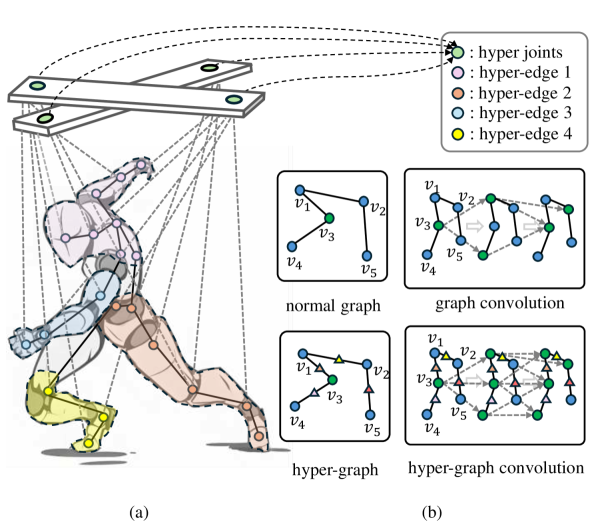
Figure 1: Illustration of our Hyper-GCN. In (a), dotted lines represent the virtual connections. Each coloured part containing multiple joints represents a hyper-graph with hyper-edges. (b) provides an intuitive comparison between normal graph convolution and hyper-graph convolution operations with the same connection degree.

To facilitate skeleton-based action recognition, both Recurrent Neural Networks (RNNs) [8, 9, 10, 11] and Convolutional Neural Networks (CNNs) [15, 16, 17] have been well explored. However, RNNs themselves cannot depict the intrinsic skeleton topology. The learned filters of CNNs, on the other hand, neglect the spatio-temporal structure of the skeleton. Drawing on these observations, recent studies have focused on how to model the skeleton topology directly.

In principle, the physical topology of human joints and bones can be consistently represented by a graph. Accordingly, the graph convolutional network (GCN) is typically introduced to achieve the aggregation of feature information conveyed by skeleton joints [18, 13, 19]. In general, two neighbouring joints can pass messages through their shared bone. In graph terms, this corresponds to the exchange of information between two vertices along their connecting edge. Besides the physical skeleton topology, attempts have been made to explore implicit relationships among joints [20, 13, 12, 19], suggesting different variants of skeleton topology. In principle, these approaches assume a binary connection between each connected vertex pair. Mathematically, the constructed topology in the adjacency matrix is represented by a normal graph. However, human actions are jointly defined by several joints. Hence, human actions encompass not only binary relations between vertex pairs but also multi-joint relationships. For instance, the action primitive starting running is manifest in the human raising the left hand while the right leg steps forward, as shown in Figure 1 (a). The binary connections are not sufficient to capture the synergistic interaction of multiple joints. This strongly argues for constructing feature aggregation paths involving multiple vertices.

Accordingly, we propose to construct a hyper-graph to depict the skeleton topology and take advantage of the outstanding performance of hyper-graph analysis techniques  [21, 22, 23, 24]. The hyper-graph topology involves multiple node connections, rather than binary connections of a normal graph. As shown in Figure 1 (a), in a hyper-graph, a hyper-edge can link more than two vertices, which has the capacity to represent complex collaborative relations among human joints. As one hyper-edge associates multiple vertices, a single hyper-graph convolution enables aggregating all the features along the hyper-edges. An illustration is provided in Figure 1 (b), where the normal graph and hyper-graph are presented to demonstrate their differences in passing the information conveyed by the vertex features.

Conceptually, for a fair comparison, we typically set each hyper-edge to contain only 2 vertices, which is the same as the normal graph. In the normal graph convolution, after 2-layer aggregation, the information of the green vertex is spread to 2 other vertices. In contrast, in a hyper-graph convolution, the information of the green vertex spreads to 4 vertices including itself, creating an extended receptive field. Theoretically, by applying a hyper-graph for modelling joint aggregation on a skeleton, improved efficiency can be obtained during learning the action semantics.

Besides its information aggregation mode, the capacity of an action recognition system is also limited by its input features. In general, the number of skeleton joints is fixed in existing benchmarks, e.g., 25 for NTU-120 [25]. The entire recognition process relies on the interactions among the involved joints. In the domain of artistic puppetry, the history of driving actions, such as Shadow Play  and Marionette  goes back more than 2000 years. This kind of art form provides an inspiration for involving additional ’hyper joints’ which can drive or facilitate a better communication between existing joints. The underlying spirit is to alleviate the pressure of the real joints in storing and transferring semantics. Jointly with the hyper joints, real joints can focus more on storing neighbouring joint features and transferring the global information to the hyper joints. Interestingly, the class token in existing Transformers can also be considered as a hyper-token  [26, 27, 28, 29]. As shown in Figure 1, the skeleton is described as a marionette, where the actions are ”controlled” by connecting hyper joints to the real joints. This suggests that the hyper joints are not only able to capture the representation information of human action, but also reveal the implicit information between physically connected joints as hints for recognition.

By endowing a hyper-graph with hyper joints, virtual connections are created to perform comprehensive hyper-graph convolutions. We construct Hyper-GCN based on the above design principles. Extensive experiments on 3 datasets, NTU RGB+D 60, NTU RGB+D 120, and NW-UCLA, are conducted for evaluation. The results validate the merits of our proposed Hyper-GCN. The main contributions are as follows:

• We propose to represent human skeleton topology by a hyper-graph. Compared with the normal graph, the efficiency of feature interaction is improved via multi-vertex aggregation.

• Virtual hyper joints are injected to connect the physical joints, enhancing the model capacity to capture the global semantics.

• We propose an adaptive hyper-graph convolution network (Hyper-GCN) for skeleton-based human action recognition. On all three public datasets used for experimentation, Hyper-GCN achieves the SOTA performance.

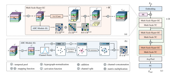
Figure 2: The framework of our Hyper-GCN. Part (a) represents the Multi-Scale Hyper-GC (MS-HGC) module, where channels are divided into 8 branches. Part (b) represents the process of constructing an adaptive hyper-graph. Part (c) represents the architecture of Hyper-GCN. $\mathbf{F}_{h}$ represents the hyper-joints which are learnable parameters. $\hat{A}_{p}$ represents the physical topology. $HA$ represents The fused topology of the adaptive hyper-graph and the human physical structure.

II Related Work

II-A Graph Topology for Action Recognition

A graph can represent a human skeleton, preserving the joint relationships via predefined edges. To aggregate semantics, GCNs have been well studied in recent years [30, 31, 32, 33, 34, 35, 36, 37, 38]. Regarding modelling the spatio-temporal relevance, ST-GCN [18] proposes to represent the topology with an adjacency matrix of 3 subsets. Similarly, 2s-AGCN [20], InfoGCN [12], and DS-GCN [14] use a self-attentive mechanism to learn the topology from joint pairs. Besides the intuitive spatio-temporal dimensions, CTR-GCN [13] proposes to learn the channel topology using subspace mappings. All the above methods construct the topology from joint pairs, which rely only on the binary relation between two vertices. In their implementation stage, the adjacency matrix is used to represent the topology. In this case, high-order information among joints is not taken into consideration, neglecting the collaborative power among multiple joints. Though hyper-graph is considered to construct topology using multivariate joint relationships, current [39, 40] solutions manually set the hyper-graphs, which greatly relies on human experience, sacrificing the adaptability of graph learning.

II-B Feature Settings for Action Recognition

It has been observed that the input features play the most essential role in delivering high recognition accuracy [41, 42, 43, 36, 44]. Drawing on this, Graph2Net [45] proposes to extract local and global spatial features jointly. Similarly, CTR-GCN [13] uses multi-scale temporal convolution to extract temporal features. While HD-GCN [19] focuses on learning the feature aggregation among different edge sets. To extend the perception field, STC-Net [46] uses the dilated kernels for graph convolution to capture the features. After all, existing GCNs [18, 20, 12, 14, 47] receive the input features from real skeleton joints. However, each skeleton joint acts as an information carrier during forward passing, which is required to deliver both local context and global semantics. Given a fixed representative capacity (number of channels), we believe it is necessary to involve additional virtual joints to balance the pressure of storing local and global information.

III Approach

III-A Preliminaries

In general, the input features in graph convolution are represented by $\mathbf{{F}_{in}}\in\mathbb{R}^{C\times T\times V}$, where $C$ represents the number of channels in the feature maps. Given the topology of a human skeleton, we usually define the graph $\mathcal{G}=(\mathcal{V},\mathcal{E})$, where $\mathcal{V}$ represents the set of joints and $\mathcal{E}$ represents the set of edges between joints. For the set of edges $\mathcal{E}$, it is formulated as an adjacent matrix $A\in\mathbb{R}^{N\times N}$, where $N$ represents the number of human joints. The normalised adjacency matrix is represented by $\hat{A}\in\mathbb{R}^{N\times N}$. The normalisation operation is formulated as follows:

$$\hat{A}=\Lambda^{-\frac{1}{2}}\ A\Lambda^{-\frac{1}{2}},$$ (1)

where $\Lambda$ represents the diagonal matrix stored with the degree of every joint. The entire normal graph convolution process can be formulated as:

$$\mathbf{F_{out}}=\sigma(\hat{A}\mathbf{F_{in}}W),$$ (2)

where $W\in\mathbb{R}^{C\times C^{\prime}}$ is the learnable parameters, representing the feature transformation patterns in the feature space. $\sigma$ denotes the non-linear activation function ReLU.

III-B Hyper-graph

Here, we use $\mathcal{G_{H}}=(\mathcal{V_{H}},\mathcal{E_{H}},\mathcal{W_{H}})$ to define the spatial hyper-graph [24] with human skeleton. $\mathcal{V_{H}}$ and $\mathcal{E_{H}}$ follow similar definitions in the normal graph, which represent the set of joints and the set of hyper-edges. In addition, we introduce $\mathcal{W_{H}}$ to represent the weights of each hyper-edge. Since a hyper-edge contains multiple joints, the corresponding topology can no longer be simply represented by an adjacency matrix. Therefore, we introduce the incidence matrix $H\in\mathbb{R}^{N\times M}$ to describe the topology of each joint in the hyper-graph. $N$ represents the number of joints and $M$ represents the number of hyper-edges. Given $v\in\mathcal{V_{H}}$ and $e\in\mathcal{E_{H}}$, the values of incidence matrix can be determined by:

$$h(e,v)=\begin{cases}1,&v\in e,\\ 0,&v\notin e\end{cases}.$$ (3)

Similar to the normal graph convolution, it also needs to normalise the hyper-graph to modulate the aggregated features. The degree of hyper-graph consists of the degree of joints and the degree of hyper-edges. The degree of joints is represented by the sum of weights of all joints contained in each hyper-edge. Given $v\in\mathcal{V_{H}}$, it can be described as follows:

$$d(v)\ =\sum_{e\in\mathcal{E_{H}}}{w(e)h(v,e)},$$ (4)

where we use a diagonal matrix $D_{v}\in\mathbb{R}^{N\times N}$ to represent the degree of joints. $W\in\mathbb{R}^{M\times M}$ represents the weight matrix of hyper-edges, which is formulated as a diagonal matrix. The degree of hyper-edges represents the sum of the number of joints contained in each hyper-edge. Given $e\in\mathcal{E_{H}}$, it can be described as follows:

$$d(e)\ =\sum_{v\in\mathcal{V_{H}}}{h(v,e)},$$ (5)

where we use a diagonal matrix $D_{e}\in\mathbb{R}^{M\times M}$ to represent the degree of hyper-edges. Therefore, the normalisation of a hyper-graph is formulated as follows:

$$\hat{H}=D_{v}^{-1}HWD_{e}^{-1}H^{T},$$ (6)

where $\hat{H}\in\mathbb{R}^{N\times N}$ represents the normalised incidence matrix for hyper-graph convolution.

III-C Adaptive Hyper-graph Construction Module

How to construct the hyper-graph is critical to better understanding human actions. As shown in Figure 2 (b), we design an Adaptive Hyper-graph Construction Module (AHC-Module). Given the feature $\mathbf{{F}^{{}^{\prime}}_{in}}\in\mathbb{R}^{C\times T\times V}$, we first perform temporal pooling, and then the obtained spatial information is the evidence to determine the optimal hyper-graph construction. This can efficiently decouple the temporal and spatial clues. After performing temporal average-pooling, we can obtain $\mathbf{\bar{F}^{{}^{\prime}}_{in}}\in\mathbb{R}^{C\times V}$. To adjust the scale of the input feature channels, we adopt a layer normalisation operation on the channel dimension. After that, we use two individual mapping functions to embed the features into the subspace for constructing the hyper-graph. This design enables preserving the original features to reflect their spatial relevance. The embedding operation can be formulated as follows:

$$P_{\textrm{emb}} =\Phi(\textrm{LN}(\textrm{Pooling}_{\textrm{T}}(\mathbf{F^{{}^{\prime}}_{in}}))),$$ (7)

$$W_{\textrm{emb}} =\textrm{Tanh}(\Psi(\textrm{LN}(\textrm{Pooling}_{\textrm{T}}(\mathbf{F^{{}^{\prime}}_{in}})))),$$ (8)

where $P_{\textrm{emb}}$ represents the relative position of the joints in the embedding space, and $W_{\textrm{emb}}$ represents the weights of hyper-edges. $\textrm{Pooling}_{\textrm{T}}$ denotes performing pooling in the temporal dimension. LN denotes the layer normalisation along the channel dimension. $\Phi\in\mathbb{R}^{C\times C_{h}},\Psi\in\mathbb{R}^{C\times 1}$ are the mapping functions of position and weight, which are set learnable parameters. $C_{h}$ represents the channels of the mapping subspace. Tanh denotes the activation function to obtain the weight of each hyper-edge, limiting the values with the range of $[-1,1]$.

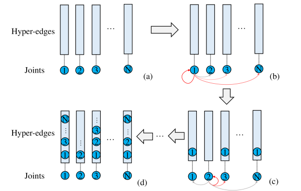
Figure 3: Illustration of the hyper-graph construction process with the proposed AHC-Module. $N$ represents the number of joints.

In the embedding space, our AHC-Module utilises the Euclidean distance to measure the joint difference. For the mapping of hyper-edges and vertices, the reason we apply only one mapping function instead of two separate ones is to ensure that vertices and hyper-edges are within the same semantic space. Define the set of joints $P_{\textrm{emb}}=\{v_{0}\in\mathbb{R}^{C_{h}},v_{1}\in\mathbb{R}^{C_{h}},...,v_{N}\in\mathbb{R}^{C_{h}}\}$, given $v_{i},v_{j}\in P_{\textrm{emb}}$, each element $m_{i,j}$ in the distance matrix $M\in\mathbb{R}^{N\times N}$ can be obtained as follows:

$$dis_{i,j}=dis_{j,i}=||v_{i}-v_{j}||^{2}_{2}.$$ (9)

In principle, we need to transform the distance matrix into a probability hyper-grap0h, which determines whether the specific joints are contained with the same hyper-edges. In order to guarantee that the model is trainable, we use the softmax operation to assign the probabilities. However, directly using the softmax would inevitably result in each joint belonging to all hyper-edges to some extent. Since this outcome is undesirable, we introduce constraints on each joint to limit the number of hyper-edges it can belong to, preventing excessive connections. We retain only the $K$ nearest hyper-edges represented by each joint in the semantic space for probability estimation. Given the row vector $\mathbf{m}_{i}$ in the distance matrix $M$, which represents the distances between joint $i$ and the other joints, we select the indices of the minimum $K$ joints from $\mathbf{m}_{i}$ and add them to the set $set^{K}_{i}$. Based on $set^{K}_{i}$, $h_{i,j}$ in the incidence matrix $H\in\mathbb{R}^{N\times N}$ of hyper-graph, can be calculated as follows:

$$h_{i,j} =\begin{cases}\frac{e^{-m_{i,j}}}{\sum_{k\in set^{K}_{i}}{e^{-m_{i,k}}}},&j\in set^{K}_{i},\\ 0,&j\notin set^{K}_{i}\end{cases}$$ (10)

The shape of our incidence matrix is consistent with the adjacency matrix of the normal graph. While our topology with hyper-graph contains more high-order information. The entire process is illustrated in the Figure 3.

III-D Multi Scale Hyper-graph Convolution

As our AHC-Module can depict the topology into a hyper-graph at different scales by adjusting the value of $K$. To accommodate the semantic information reflected by these varying scales, we further propose the Multi-Scale Hyper-graph Convolution (MS-HGC), as shown in Figure 2 (a). We use different branches to independently perform hyper-graph convolution on the topological information represented by the multi-scale hyper-graphs, thereby enhancing the computational efficiency of the Hyper-GCN.

Besides the hyper-graph, we incorporate the physical topology to emphasise the natural physical relations of a human being’s skeleton. To achieve this objective, existing methods [18, 20, 13, 19] divide the physical topology of the human body into 3 subsets. They are represented by $S=\{s_{id},s_{cf},s_{cp}\}$, where $s_{id}$, $s_{cf}$ and $s_{cp}$ denote the identity, centrifugal, and centripetal joint subsets. In our MS-HGC, to ensure that the integrated physical topology in each branch remains complete, we merge them into a single set. We divide the input feature into 8 separate branches along the channel dimension, which are processed by 8 MS-HGC parallelly, delivering 8 multi-scale hyper-graphs. 8 branches are aggregated by channel concatenation after the hyper-graph convolutions, as shown in Figure 2 (a). The operation of MS-HGC can be formulated as follows:

$$\mathbf{F_{out}} =\uplus^{8}_{i=1}{(\hat{A_{i}}+\alpha_{i}\cdot\hat{H_{i}})\mathbf{F^{[(i-1)\times C^{{}^{\prime}}+1,...,i\times C^{{}^{\prime}}]}_{in}}W_{i}},$$ (11)

where $\mathbf{[(i-1)\times C^{{}^{\prime}}+1,...,i\times C^{{}^{\prime}}]}$ represents the channels of $\mathbf{F_{in}}$. $\uplus$ represents the channel concatenation. $\hat{A_{i}}$ and $\hat{H_{i}}$ denote the normalized physical adjacency matrix and normalized incidence matrix. $W_{i}$ and $\alpha_{i}$ are the learnable parameters for each branch.

III-E Virtual Connections

It is worth emphasising that incorporating learnable joints among different samples is essential for enhancing the model capacity, as these learnable joints capture generalised features of human actions. This not only enriches the semantic information but also facilitates easier interaction connections among real joints. Therefore, we introduce the hyper-joints which are to participate in the hyper-graph convolution as shown in Figure 2 (a). The shape of hyper-joints is consistent with the feature $\mathbf{F_{p}}\in\mathbb{R}^{C^{{}^{\prime}}\times T\times V}$, which is described as $\mathbf{F_{h}}\in\mathbb{R}^{C^{{}^{\prime}}\times T\times V_{h}}$. Specifically, the learning of hyper-joints is supervised by the loss function, which guides these hyper-joints to support generalisable driven features embedded within large amounts of data. Furthermore, we set independent hyper-joints at each layer of Hyper-GCN, aiming to harmonise features at different depths. Typically, these hyper-joints are involved in spatial hyper-graph convolution rather than in temporal convolution.

To diversify these hyper-joints, we propose the Divergence Loss for hyper-joints optimisation to mitigate their homogenisation. We adopt a cosine matrix $C\in\mathbb{R}^{V_{h}\times V_{h}}$ to measure the differences between hyper-joints, which can be formulated as follows:

$$C=\frac{\text{ReLU}(\mathbf{F_{h}F^{T}_{h}})}{||\mathbf{F_{h}}||^{2}}-\mathbf{I},$$ (12)

where $\mathbf{I}$ represents the identity matrix which is used to emphasise the irrelevance between each learned hyper-joint pair.

Specifically, in Divergence Loss, we measure the differences of hyper-joints with the mean of the cosine matrix $C$ in each layer. The calculation can be formulated as:

$$\mathcal{L}_{h}(C) =\frac{\sum^{V_{h}}_{i=1}\sum^{V_{h}}_{j=1}c_{i,j}}{(V_{h}-1)^{2}},\quad c_{i,j}\in C,$$ (13)

$$\mathcal{L} =\mathcal{L}_{CE}+\frac{1}{L}\sum^{L}_{l=1}L_{h}(C_{l}),$$ (14)

where $V_{h}$ represents the number of hyper-joints we introduced. $C_{l}$ represents the cosine matrix of the $l$-th layer. Additionally, to preserve the original physical topology, we use the AHC-Module solely to learn the topology between feature $\mathbf{F_{h}}$ and feature $\mathbf{F_{p}}$.

III-F Entire Architecture

Hyper-GCN consists of an embedding layer, 9 spatial-temporal convolution layers, a global average pooling, and an FC layer, as shown in Figure 2 (c).

The embedding layer is utilised to map individual joints into a high-dimensional feature space for subsequent adaptive hyper-graph convolution. To preserve the position awareness of the embedded features, we introduce the position embedding in the embedding layer inspired by InfoGCN [12].

The 9 layers of Hyper-GCN are categorised into 3 stages. Each stage consists of 3 layers. Each layer consists of Multi-Scale Hyper-graph convolution (MS-HGC) and Multi-Scale Temporal convolution (MS-TC) [13]. In stage 1, the number of channels is set as 128. Then it increases to 256 for stage 2 and stage 3.

Dense connections are introduced to integrate deep and shallow features in each stage, which can smooth the obtained distribution against the hyper-vertices interaction at each layer.

Methods	Publication	Modalities	GFLOPs	Params (M)	NTU-RGB+D 60		NTU-RGB+D 120		NW-UCLA (%)
					X-Sub (%)	X-View (%)	X-Sub (%)	X-Set (%)
ST-GCN [18]	AAAI 2018	J+B	-	-	81.5	88.3	70.7	73.2	-
2s-AGCN [20]	CVPR 2019	J+B	-	-	88.5	95.1	82.5	84.2	-
DGNN [32]	CVPR 2019	J+B+JM+BM	-	-	89.9	96.1	-	-	-
SGN [30]	CVPR 2020	J+B+JM+BM	-	-	89.0	94.5	79.2	81.5	92.5
DC-GCN+ADG [33]	ECCV 2020	J+B+JM+BM	1.83	4.9	90.8	96.6	86.5	88.1	95.3
DDGCN [31]	ECCV 2020	J+B+JM+BM	-	-	91.1	97.1	-	-	-
MS-G3D [42]	CVPR 2020	J+B+JM+BM	5.22	2.8	91.5	96.2	86.9	88.4	-
MST-GCN [34]	AAAI 2021	J+B+JM+BM	-	12.0	91.5	96.6	87.5	88.8	-
CTR-GCN [13]	ICCV 2021	J+B+JM+BM	1.97	1.5	92.4	96.4	88.9	90.6	96.5
EfficientGCN-B4 [43]	TPAMI 2022	J+B+JM+BM	15.2	2.0	91.7	95.7	88.3	89.1	-
InfoGCN* [12]	CVPR 2022	J+B+J’+B’	1.84	1.6	92.7	96.9	89.4	90.7	96.6
FR Head [48]	CVPR 2023	J+B+JM+BM	-	2.0	92.8	96.8	89.5	90.9	96.8
HD-GCN* [19]	ICCV 2023	J+B+J’+B’	1.77	1.7	93.0	97.0	89.8	91.2	96.9
DS-GCN [14]	AAAI 2024	J+B+JM+BM	-	-	93.1	97.5	89.2	90.3	-
Hyper-GCN (w/o ensemble)	-	J	1.62	1.0	91.1	95.3	87.0	88.4	94.8
Hyper-GCN (2-ensemble)	-	J+B	1.62	1.0	92.9	96.3	89.8	90.9	96.2
Hyper-GCN (4-ensemble)	-	J+B+JM+BM	1.62	1.0	93.1	96.7	90.2	91.4	96.6

TABLE I: Comparison of Hyper-GCN with advanced solutions on NTU-RGB+D 60, NTU-RGB+D 120, and NW-UCLA datasets. For a fair comparison, we use a 4-streams ensemble to evaluate the performance of the mentioned methods. J, B, JB, and JM represent the joint, bone, joint motion, and bone motion. In addition, for InfoGCN, HD-GCN [12, 19], we use the results from 4-streams according to the original papers for a fair comparison. GFLOPs and Params (M) all represent the single-stream.

IV Evaluation

In this section, we conduct extensive experiments on standard benchmarking datasets to evaluate our Hyper-GCN, in the task of skeleton-based human action recognition.

IV-A Datasets

NTU-RGB+D 60 NTU-RGB+D 60 [11] is a large dataset widely used in skeleton-based human action recognition. It consists of 56,880 different samples, categorised into 60 classes, obtained from the directed performances of 40 different actors. There are two 2 evaluation benchmarks. (1) Cross-Subject (X-Sub): For the 40 actors, 20 are used for training and 20 for validation. (2) Cross-view (X-View): For 3 views, 2 are used for training, and 1 for validation.

NTU-RGB+D 120 NTU-RGB+D 120 [25] is am extention of NTU 60, which introduce 57,367 new action samples. It consists of 114,480 different samples, categorised into 120 classes instead of 60 classes. The number of actors increase to 106. It also corresponds yo 2 benchmarks. (1) Cross-Subject (X-Sub): For the 106 actors, 53 are used for training and 53 for validation. (2) Cross-Setup (X-Set): For the 32 setups, the sample with even setup IDs are used for training, and the odd setup IDs for validation.

Northwestern-UCLA. The Northwestern-UCLA (NW-UCLA) dataset [49] contains 1494 video clips, which is categorised into 10 classes. It is obtained through 3 cameras with different camera views and is performed by 10 actors. As the proposed benchmark, for 3 camera views, 2 camera views are used for training, and the remaining 1 is used for validation.

IV-B Implementation Details

Our training and evaluation stages are on a single RTX 3090 GPU. In terms of the training phase, Hyper-GCN is optimised by Stochastic Gradient Descent (SGD) with Nesterov momentum set at 0.9 and a weight decay at 0.0004. Our implementation uses label smooth cross-entropy loss with the Divergence Loss we proposed. We set a total of 140 epochs with the start 5 warm-up epochs. The initial learning rate is 0.05, which is reduced to 0.005 at epoch 110 and to 0.0005 at epoch 120. The training batch size is set to 64 for NTU RGB+D and NTU RGB+D 120, and 16 for Northwestern-UCLA.

IV-C Comparison with the State-of-the-Art

Multi-stream ensembles proposed in  [50] have been proven effective by most of the existing state-of-the-art methods. We also use a 4-streams ensemble to evaluate our model.

The detailed results are reported in Table I. To the best of our knowledge, a comparison with SOTA shows that our proposed Hyper-GCN achieves the SOTA level on each dataset. Especially, we outperform the involved competitors on NTU-RGB+D 120. This demonstrates the effectiveness and merits of Hyper-GCN.

IV-D Ablation Study

We conduct ablation experiments and report visualisations to analyse the effectiveness of each component of our design. All the ablation study is evaluated on the benchmark of NTU-RGB+D 120, using the joint modality. The Baseline for comparison is set by replacing the MS-HGC with vanilla GC, and removing the hyper-joints and dense connections in the backbone.

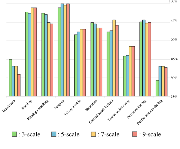
Figure 4: Top-1 accuracy in selected classes. The $K$-scale represents the $K$-scale hyper-graph in MS-HGC. The data is displayed starting from 75%.

	$K$-scale	NTU RGB+D 120 X-Sub (%)
Baseline	-	85.1
Single scale	3	86.4 ($\uparrow$ 1.3)
	5	86.5 ($\uparrow$ 1.4)
	7	86.5 ($\uparrow$ 1.4)
	9	86.3 ($\uparrow$ 1.2)
Multi scale	[0,2,3,4,5,6,7,8]	86.6 ($\uparrow$ 1.5)
	[2,3,4,5,6,7,8,9]	86.7 ($\uparrow$ 1.6)
	[3,4,5,6,7,8,9,10]	86.6 ($\uparrow$ 1.5)

TABLE II: Comparison of the hyper-parameter $K$ in terms of adaptive hyper-graph construction. [$k_{1}$,$k_{2}$,…,$k_{8}$] represents the $K$-scale hyper-graph of 8 branches in MS-HGC. The bold font represents the best results.

Multi-Scale Hyper-graph: As we mentioned, Multi-Scale Hyper-graph Convolution (MS-HGC) consists of an 8-branch parallel architecture. In particular, each branch corresponds to a hyper-graph at a different scale. The hyper-graphs at different scales represent the maximum number of hyper-edges each joint is contained in. They reflect the varying degrees of aggregation in the constructed topology. The different scales of hyper-graphs are determined by the hyper-parameter $K$ that we define. Therefore, to explore how to set the hyper-parameter $K$ for the branches in MS-HGC, we design the ablation experiments to investigate the impact of different scales on the model’s recognition ability, as well as to compare the results by defining a single scale.

The results are reported in Table II. When $K$ equals 1, each hyper-edge contains only one joint, which essentially eliminates any interaction between joints. Therefore, we do not set K to 1. Observing the design of the single scale hyper-graph, it becomes clear that increasing $K$ does not always yield better performance. A very large $K$ means that the maximum number of hyper-edges each joint is contained in increases, which in turn causes the number of joints in each hyper-edge to grow. Even though these ”extra” joints may be optimised for minimal weight, they are likely to act as ”noise”, disrupting the information interaction represented by the hyper-edge.

Furthermore, compared to a single-scale design, it is evident that the multi-scale design of MS-HGC outperforms the single scale design. For the complex and diverse characteristics of human action, multi-scale hyper-graphs in the spatial dimension can better capture features at multiple levels. Therefore, we visualise the Top-1 accuracy of selected human action categories as shown in Figure 4. This is especially advantageous for recognising actions with varying degrees of motion. For instance, for actions like ”Brushing teeth” or ”Salutation”, where only local joints are in motion, the smaller-scale hyper-graphs focus more on the local joints. In contrast, for actions like ”Stand up” and ”Jump up”, where the entire body is engaged, a larger-scale hyper-graph can capture information between distant joints. This also inspired us to adopt the AHC-Module in different branches to complementarily learn hyper-graph topology at different scales.

	NTU RGB+D 120 X-Sub (%)	GFLOPs	Parmas (M)
Baseline	85.1	1.70	1.52
w/ MS-HGC	86.6 ($\uparrow$ 1.5)	1.59	1.03
w/ 1	86.7 ($\uparrow$ 1.6)	1.61	1.03
w/ 2	86.9 ($\uparrow$ 1.8)	1.62	1.04
w/ 3	87.0 ($\uparrow$ 1.9)	1.62	1.05
w/ 4	86.6 ($\uparrow$ 1.5)	1.64	1.05
w/ 5	86.4 ($\uparrow$ 1.3)	1.66	1.06

TABLE III: The comparison of the configurations of hyper joints. w/ $N$ represents the number of hyper joints in each layer. These experiments are conducted in the setting w/ MS-HGC. The bold font represents the best results.

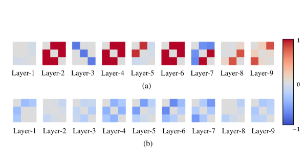
Figure 5: The comparison of the cosine matrices of hyper-joints. The matrix elements range from $[-1,1]$. This experiment is set w/ 3 hyper-joints. Part (a) represents w/o Divergence Loss. Part (b) represents w/ Divergence Loss. The cosine matrix is calculated by Eqn. 12.

Virtual Connections: We conduct the ablation study to analyse the hyper joints with the Divergence Loss. The results are listed in Table III. By comparison, the performance is not monotonically increasing with the number of hyper joints. The case of introducing only 3 hyper joints achieves the best performance. As our hyper joints are learned from a large amount of data, too many hyper joints can introduce redundant and ambiguous clues, weakening the model capacity. Besides, the involvement of hyper joints delivers consistent improvement, while introducing only a marginal increase in terms of model size and complexity.

In addition, we visualised the cosine matrices in certain layers of Hyper-GCN, as shown in Figure 5. Clearly, in the absence of the Divergence Loss, the homogenisation of the learned hyper-joints in several layers is severe. This can limit the ability of hyper-joints to represent the generalised features of human actions. The observation further validates the effectiveness of the Divergence Loss for hyper-joint optimisation, supporting our viewpoint that generalised features with a certain degree of differentiation are needed to participate in hyper-graph convolution.

Method	S-1	S-2	S-3	MS-HGC	H	NTU-RGB+D 120
						X-Sub
Baseline						84.8
	$\checkmark$					84.8
		$\checkmark$				84.8
			$\checkmark$			84.9 ($\uparrow$ 0.1)
Hyper-GCN	$\checkmark$	$\checkmark$				84.9 ($\uparrow$ 0.1)
		$\checkmark$	$\checkmark$			85.0 ($\uparrow$ 0.2)
	$\checkmark$	$\checkmark$	$\checkmark$			85.1 ($\uparrow$ 0.3)
	$\checkmark$	$\checkmark$	$\checkmark$	$\checkmark$		86.6 ($\uparrow$ 2.0)
	$\checkmark$	$\checkmark$	$\checkmark$	$\checkmark$	$\checkmark$	87.0 ($\uparrow$ 2.4)

TABLE IV: The ablation study of architecture settings. S-$i$ represents adding dense connection in stage $i$. MS-HGC and H represent w/ MS-HGC and w/ 3 hyper-joints.

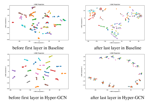
Figure 6: t-SNE visualisation of Baseline and Hyper-GCN. Different colours represent the features of different joints.

Architecture of Backbone: We validate the effectiveness of performing dense connections in the backbone. The experimental results are collected in Table IV. The dense connections in the experiments are only added within each stage. It is observed that dense connections in shallow layers do not improve the performance as much as in deep layers. As the layers go deeper, the number of channels gradually increases and the variance of information extracted from each layer becomes steeper. This suggests that the deeper stages require dense connections to modulate the variance between features. For example, the performance introducing dense connections at stage 1 and stage 2 is close to adding the dense connection only at stage 3.

To further validate that Hyper-GCN increases the efficiency of information interaction, we perform t-SNE projections on the output features of each layer, as shown in Figure 6. Notice that the semantic information represented by the last layer features of Hyper-GCN is very convergent. This represents that the semantic information of each joint is adequately conveyed in Hyper-GC. The joints with similar semantic can prevent sacrificing the information after global average pooling.

V Conclusion

In this paper, we propose a Hyper-graph Convolutional Network for skeleton-based human action recognition. To exploit the implicit topology of multivariate synergy between joints, we introduce Multi-Scale Hyper-graph Convolution and virtual connections. We also introduce dense connections to fuse shallow and deep features. We carry out experiments on the dataset NTU-RGB+D 60 & 120, NW-UCLA to validate the effectiveness of Hyper-GCN. The experimental analysis verifies that our design can improve the recognition performance. To the best of our knowledge, Hyper-GCN achieves the SOTA performance on 3 public datasets. The involvement of hyper-graph modelling indeed extends existing GCN-based action recognition paradigms.

References

- [1] A. S. Nikam and A. G. Ambekar, “Sign language recognition using image based hand gesture recognition techniques,” in 2016 Online International Conference on Green Engineering and Technologies, 2016, pp. 1–5.
- [2] C. I. Nwakanma, F. B. Islam, M. P. Maharani, D.-S. Kim, and J.-M. Lee, “Iot-based vibration sensor data collection and emergency detection classification using long short term memory,” in International Conference on Artificial Intelligence in Information and Communication, 2021, pp. 273–278.
- [3] C. Huesser, S. Schubiger, and A. Çöltekin, “Gesture interaction in virtual reality: A low-cost machine learning system and a qualitative assessment of effectiveness of selected gestures vs. gaze and controller interaction,” in International Conference on Human-Computer Interaction. Berlin, Heidelberg: Springer-Verlag, 2021, p. 151–160. [Online]. Available: https://doi.org/10.1007/978-3-030-85613-7_11
- [4] P. K. Mishra, A. Mihailidis, and S. S. Khan, “Skeletal video anomaly detection using deep learning: Survey, challenges, and future directions,” IEEE Transactions on Emerging Topics in Computational Intelligence, 2024.
- [5] B. Omarov, S. Narynov, Z. Zhumanov, A. Gumar, and M. Khassanova, “A skeleton-based approach for campus violence detection.” Computers, Materials & Continua, vol. 72, no. 1, 2022.
- [6] A. Taha, H. H. Zayed, M. Khalifa, and E.-S. M. El-Horbaty, “Skeleton-based human activity recognition for video surveillance,” International Journal of Scientific & Engineering Research, vol. 6, no. 1, pp. 993–1004, 2015.
- [7] B. Lee, M. Lee, P. Zhang, A. Tessier, and A. Khan, “Semantic human activity annotation tool using skeletonized surveillance videos,” in Proceedings of the 2019 ACM International Symposium on Wearable Computers, 2019, pp. 312–315.
- [8] Y. Du, W. Wang, and L. Wang, “Hierarchical recurrent neural network for skeleton based action recognition,” in CVPR, 2015, pp. 1110–1118.
- [9] V. Veeriah, N. Zhuang, and G.-J. Qi, “Differential recurrent neural networks for action recognition,” in ICCV, 2015, pp. 4041–4049.
- [10] J. Liu, A. Shahroudy, D. Xu, A. C. Kot, and G. Wang, “Skeleton-based action recognition using spatio-temporal lstm network with trust gates,” TPAMI, vol. 40, no. 12, pp. 3007–3021, 2018.
- [11] A. Shahroudy, J. Liu, T.-T. Ng, and G. Wang, “Ntu rgb+d: A large scale dataset for 3d human activity analysis,” in CVPR, 2016, pp. 1010–1019.
- [12] H.-G. Chi, M. H. Ha, S. Chi, S. W. Lee, Q. Huang, and K. Ramani, “Infogcn: Representation learning for human skeleton-based action recognition,” in CVPR, 2022, pp. 20 154–20 164.
- [13] Y. Chen, Z. Zhang, C. Yuan, B. Li, Y. Deng, and W. Hu, “Channel-wise topology refinement graph convolution for skeleton-based action recognition,” in ICCV, 2021, pp. 13 339–13 348.
- [14] J. Xie, Y. Meng, Y. Zhao, A. Nguyen, X. Yang, and Y. Zheng, “Dynamic semantic-based spatial graph convolution network for skeleton-based human action recognition,” AAAI, vol. 38, no. 6, pp. 6225–6233, Mar. 2024. [Online]. Available: https://ojs.aaai.org/index.php/AAAI/article/view/28440
- [15] G. Chéron, I. Laptev, and C. Schmid, “P-cnn: Pose-based cnn features for action recognition,” in ICCV, 2015, pp. 3218–3226.
- [16] K. Simonyan and A. Zisserman, “Two-stream convolutional networks for action recognition in videos,” in NIPS, ser. NIPS’14. Cambridge, MA, USA: MIT Press, 2014, p. 568–576.
- [17] S. Ji, W. Xu, M. Yang, and K. Yu, “3d convolutional neural networks for human action recognition,” TPAMI, vol. 35, no. 1, pp. 221–231, 2012.
- [18] S. Yan, Y. Xiong, and D. Lin, “Spatial temporal graph convolutional networks for skeleton-based action recognition,” in AAAI, 2018.
- [19] J. Lee, M. Lee, D. Lee, and S. Lee, “Hierarchically decomposed graph convolutional networks for skeleton-based action recognition,” in ICCV, 2023, pp. 10 410–10 419.
- [20] L. Shi, Y. Zhang, J. Cheng, and H. Lu, “Two-stream adaptive graph convolutional networks for skeleton-based action recognition,” in CVPR, 2019, pp. 12 018–12 027.
- [21] J. Jiang, Y. Wei, Y. Feng, J. Cao, and Y. Gao, “Dynamic hypergraph neural networks.” in IJCAI, 2019, pp. 2635–2641.
- [22] S. Bai, F. Zhang, and P. H. Torr, “Hypergraph convolution and hypergraph attention,” Pattern Recognition, vol. 110, p. 107637, 2021.
- [23] G. Karypis, R. Aggarwal, V. Kumar, and S. Shekhar, “Multilevel hypergraph partitioning: Application in vlsi domain,” in Proceedings of the 34th annual Design Automation Conference, 1997, pp. 526–529.
- [24] Y. Gao, Y. Feng, S. Ji, and R. Ji, “Hgnn+: General hypergraph neural networks,” TPAMI, vol. 45, no. 3, pp. 3181–3199, 2023.
- [25] J. Liu, A. Shahroudy, M. Perez, G. Wang, L.-Y. Duan, and A. C. Kot, “Ntu rgb+d 120: A large-scale benchmark for 3d human activity understanding,” IEEE Trans. Pattern Anal. Mach. Intell., vol. 42, no. 10, p. 2684–2701, oct 2020. [Online]. Available: https://doi.org/10.1109/TPAMI.2019.2916873
- [26] H. Qiu, B. Hou, B. Ren, and X. Zhang, “Spatio-temporal segments attention for skeleton-based action recognition,” Neurocomputing, vol. 518, pp. 30–38, 2023.
- [27] L. Wang and P. Koniusz, “3mformer: Multi-order multi-mode transformer for skeletal action recognition,” in CVPR, 2023, pp. 5620–5631.
- [28] Q. Wang, S. Shi, J. He, J. Peng, T. Liu, and R. Weng, “Iip-transformer: Intra-inter-part transformer for skeleton-based action recognition,” in BigData, 2023, pp. 936–945.
- [29] W. Xin, Q. Miao, Y. Liu, R. Liu, C.-M. Pun, and C. Shi, “Skeleton mixformer: Multivariate topology representation for skeleton-based action recognition,” in ACM MM, ser. MM ’23. New York, NY, USA: Association for Computing Machinery, 2023, p. 2211–2220. [Online]. Available: https://doi.org/10.1145/3581783.3611900
- [30] P. Zhang, C. Lan, W. Zeng, J. Xing, J. Xue, and N. Zheng, “Semantics-guided neural networks for efficient skeleton-based human action recognition,” in CVPR, 2020, pp. 1109–1118.
- [31] M. Korban and X. Li, “Ddgcn: A dynamic directed graph convolutional network for action recognition,” in ECCV. Berlin, Heidelberg: Springer-Verlag, 2020, p. 761–776. [Online]. Available: https://doi.org/10.1007/978-3-030-58565-5_45
- [32] L. Shi, Y. Zhang, J. Cheng, and H. Lu, “Skeleton-based action recognition with directed graph neural networks,” in CVPR, 2019, pp. 7904–7913.
- [33] K. Cheng, Y. Zhang, C. Cao, L. Shi, J. Cheng, and H. Lu, “Decoupling gcn with dropgraph module for skeleton-based action recognition,” in ECCV. Berlin, Heidelberg: Springer-Verlag, 2020, p. 536–553. [Online]. Available: https://doi.org/10.1007/978-3-030-58586-0_32
- [34] D. Feng, Z. Wu, J. Zhang, and T. Ren, “Multi-scale spatial temporal graph neural network for skeleton-based action recognition,” IEEE Access, vol. 9, pp. 58 256–58 265, 2021.
- [35] M. Li, S. Chen, X. Chen, Y. Zhang, Y. Wang, and Q. Tian, “Actional-structural graph convolutional networks for skeleton-based action recognition,” in CVPR, 2019, pp. 3595–3603.
- [36] T. Ahmad, L. Jin, L. Lin, and G. Tang, “Skeleton-based action recognition using sparse spatio-temporal gcn with edge effective resistance,” Neurocomputing, vol. 423, pp. 389–398, 2021.
- [37] J. Zhang, G. Ye, Z. Tu, Y. Qin, Q. Qin, J. Zhang, and J. Liu, “A spatial attentive and temporal dilated (satd) gcn for skeleton-based action recognition,” CAAI Transactions on Intelligence Technology, vol. 7, no. 1, pp. 46–55, 2022.
- [38] Q. Wang, K. Zhang, and M. A. Asghar, “Skeleton-based st-gcn for human action recognition with extended skeleton graph and partitioning strategy,” IEEE Access, vol. 10, pp. 41 403–41 410, 2022.
- [39] Y. Zhu, G. Huang, X. Xu, Y. Ji, and F. Shen, “Selective hypergraph convolutional networks for skeleton-based action recognition,” in ICMR, ser. ICMR ’22. New York, NY, USA: Association for Computing Machinery, 2022, p. 518–526. [Online]. Available: https://doi.org/10.1145/3512527.3531367
- [40] X. Hao, J. Li, Y. Guo, T. Jiang, and M. Yu, “Hypergraph neural network for skeleton-based action recognition,” TIP, vol. 30, pp. 2263–2275, 2021.
- [41] K. Cheng, Y. Zhang, X. He, W. Chen, J. Cheng, and H. Lu, “Skeleton-based action recognition with shift graph convolutional network,” in CVPR, 2020, pp. 180–189.
- [42] Z. Liu, H. Zhang, Z. Chen, Z. Wang, and W. Ouyang, “Disentangling and unifying graph convolutions for skeleton-based action recognition,” in CVPR, 2020, pp. 140–149.
- [43] Y.-F. Song, Z. Zhang, C. Shan, and L. Wang, “Constructing stronger and faster baselines for skeleton-based action recognition,” TPAMI, vol. 45, no. 2, pp. 1474–1488, 2022.
- [44] L. Huang, Y. Huang, W. Ouyang, and L. Wang, “Part-level graph convolutional network for skeleton-based action recognition,” in AAAI, vol. 34, no. 07, 2020, pp. 11 045–11 052.
- [45] C. Wu, X.-J. Wu, and J. Kittler, “Graph2net: Perceptually-enriched graph learning for skeleton-based action recognition,” TCSVT, vol. 32, no. 4, pp. 2120–2132, 2022.
- [46] J. Lee, M. Lee, S. Cho, S. Woo, S. Jang, and S. Lee, “Leveraging spatio-temporal dependency for skeleton-based action recognition,” in ICCV, 2023, pp. 10 221–10 230.
- [47] R. Hou, Z. Wang, R. Ren, Y. Cao, and Z. Wang, “Multi-channel network: Constructing efficient gcn baselines for skeleton-based action recognition,” Computers & Graphics, vol. 110, pp. 111–117, 2023.
- [48] H. Zhou, Q. Liu, and Y. Wang, “Learning discriminative representations for skeleton based action recognition,” in CVPR, 2023, pp. 10 608–10 617.
- [49] J. Wang, X. Nie, Y. Xia, Y. Wu, and S.-C. Zhu, “Cross-view action modeling, learning, and recognition,” in CVPR, ser. CVPR ’14. USA: IEEE Computer Society, 2014, p. 2649–2656. [Online]. Available: https://doi.org/10.1109/CVPR.2014.339
- [50] L. Shi, Y. Zhang, J. Cheng, and H. Lu, “Skeleton-based action recognition with multi-stream adaptive graph convolutional networks,” TIP, vol. 29, pp. 9532–9545, 2020.