On the non-hermitian Kitaev chain

Abstract

We study the non-hermitian Kitaev chain model, for arbitrary complex parameters. In particular, we give a concise characterisation of the curves of eigenvalues in the complex plane in the infinite size limit. Using this solution, we characterise under which conditions the skin effect is absent, and for which eigenstates this is the case. We also fully determine the region in parameter space for which the model has a zero mode.

I Introduction

The study of non-hermitian systems, in various contexts, has been extremely intense during the last years. These studies cover the properties of non-hermitian systems in general (focussing on the differences and similarities with hermitian systems), studies of particular non-hermitian models, as well as utilising non-hermitian systems for actual applications, using various different types of physical systems BeBuKu2019 ; BrLiBeRoAr2022unpub ; Br2014 ; DeYoHa2021 ; Ed2022 ; EdKuBe2019 ; GoAsKaTaHiUe2018 ; KaBeSa2019 ; KaShUeSa2019 ; KoBu2020 ; KuDw2019 ; KuEdBuBe2018 ; MaBe2021 ; MaVaTo2018 ; LaQv2023 ; Le2016 ; LeLiGo2019 ; LeBlHuChNo2017 ; LiWaDuCh2024unpub ; LiWeWuRuChLeNi2024unpub ; LiLi2024 ; LiTaYaLiLe2023 ; LiLiAn2023 ; MaAuPePaAc2024 ; MoArBe2023 ; NeRo2024 ; OkKaShSa2020 ; OrHe2023 ; RaSiRaJi2024unpub ; RiRo2022 ; RoOrAgHe2024 ; SaCiCABa2024 ; ShZhFu2018 ; StBe2021 ; VyRo2021 ; YaBe2024unpub ; YaMa2023 ; YaMoBe2023 ; YaWa2018 ; YoPeKaHa2019 ; XiDeWaZhWaYiXu2019 ; Xi2018 ; ZeBe2024 ; ZhSoZhZhLiCaLi2024 ; ZhLe2019 . One aspect that is of particular relevance for the current paper is the presence of the skin-effect, which is closely related to the breakdown of the famed bulk boundary correspondence of hermitian topological systems HeBaRe2019 ; Lo2019 ; LeTh2019 ; LiZhAiGoKaUeNo2019 ; FlZoVaBeBaTi2022 ; ZiReRo2021 ; BoKrSl2020 ; YoMu2019 ; YaMoBe2021 ; EdKuYoBe2020 ; Sc2020 ; BrHy2019 ; EdAr2022 .

In this paper, we focus solely on Kitaev chain Ki2001 famous for its Majorana zero modes in its topological phase (see Al2012 for a review). We consider the non-hermitian version of this model, which has, in various incarnations, been studied before Yu2017 ; KlCaDaMaWu2017 ; LiZhZhSo2018 ; LiJiSo2020 ; KaAsKaUe2018 ; Li2019 ; YaSo2020 ; ZhGuKoZhLi2021 ; SaNiTa2022 ; SaLa2023 ; ShSo2023 ; LiWaSoWa2024 ; RaRoKuKaSa2023 ; Zh2024 ; MoNa2024 ; FuKaMo2024 ; PiMeAg2024unpub ; CaAg2024unpub ; LiLiZhTiArLi2024 . We concisely characterise the location of the eigenvalues in the complex plane in the limit for an open chain in the infinite system size. It is clearly natural to ask for which general choice of parameters does the non-hermitian Kitaev chain have a zero-mode. Interestingly, the full answer to this question is arguably a bit more complicated than one might expect.

The eigenvalues of generic non-hermitian systems are known to be very sensitive to the boundary conditions KuEdBuBe2018 ; KoBu2020 . This is due to the skin effect. Eigenstates exhibiting the skin effect are localised at the boundary of the system, with an amplitude that decays exponentially in the bulk of the system. Because of this exponential localisation of the eigenstates near the boundary, it is clear that the system will be sensitive to small changes in the boundary conditions. In addition, the usual algorithms to obtain the eigenvalues numerically becomes unstable for large system sizes. For one-dimensional systems, one can use knowledge of the periodic system in order to predict whether or not the open system exhibit skin-effect or not. In particular, one considers the eigenvalues of the periodic system, and determines if this winds around an arbitrary point GoAsKaTaHiUe2018 ; KaShUeSa2019 ; OkKaShSa2020 . If such a winding exists, the system exhibits a skin effect. It is, however, not a priori clear for which choices of parameters in the model this occurs, and if it occurs, to which eigenvalues it pertains. Because of this, it is interesting to find an exact solution of the non-hermitian model one studies. By this we mean a concise characterisation of the eigenvalues, that can be easily solved numerically, without stability issues.

In the current paper, we provide explicit answers to the questions we posed above for the non-hermitian Kitaev chain. We introduce the non-hermitian Kitaev chain, in order to set the notation, and start with the general analysis to solve the model in Sec. II. We continue in Sec. III by providing the solution of the non-hermitian Kitaev chain, for chains of finite length, under the restriction that the left and right hopping parameters $t_{1}$ and $t_{2}$ are equal. In Sec. IV we give a complete characterisation of the parameters, for which the (non-hermitian) model has a zero-mode. Here, we directly work in the infinite system size limit. In Sec. V, we provide a concise characterisation of the eigenvalues of the model, again for fully generic parameters, in the infinite system size limit. Using this characterisation, one can easily obtain the curves in the complex plain corresponding to the eigenvalues of the model. In Sec. VI, we analyse the solution to determine under which conditions the model exhibits skin effect, and if this is the case, to which eigenvalues this pertains. In Sec. VII we briefly discuss our results.

II The non-hermitian Kitaev chain

In this section we state the model we are interested in, namely the Kitaev chain with nearest neighbour hopping and pairing, for arbitrary, complex parameters and start with the analysis to find the eigenvalues. We are mainly interested in open chains, with ‘free’ boundary conditions. In this paper, we do not study the transition from the open to the periodic system. In terms of fermion creation and annihilation operators, $c_{j}^{\dagger}$, $c_{j}$, the model for $L$ sites reads

$$H=\sum_{j=1}^{L}\frac{m}{2}\bigl{(}c_{j}^{\dagger}c_{j}-c_{j}c_{j}^{\dagger}\bigr{)}+\sum_{j=1}^{L-1}\Bigl{(}t_{1}c_{j}^{\dagger}c_{j+1}+t_{2}c_{j+1}^{\dagger}c_{j}+d_{1}c_{j}^{\dagger}c_{j+1}^{\dagger}+d_{2}c_{j+1}c_{j}\Bigr{)}\ .$$ (1)

To analyse the model, we write the hamiltonian in Bogoliubov-de Gennes form, that is, we write

$$H=\frac{1}{2}\Psi^{\dagger}\cdot\mathcal{H}_{\rm BdG}\cdot\Psi\ ,$$ (2)

where $\Psi^{\dagger}=(c_{1}^{\dagger},c_{1},c_{2}^{\dagger},c_{2},\ldots)$. For the model Eq. (1), we find that $\mathcal{H}_{\rm BdG}$ is the following $2L\times 2L$ matrix

$$\mathcal{H}_{\rm BdG}=\begin{pmatrix}m&0&t_{1}&d_{1}&0&0&\cdots&\cdots&0&0\\ 0&-m&-d_{2}&-t_{2}&0&0&\cdots&\cdots&0&0\\ t_{2}&-d_{1}&m&0&t_{1}&d_{1}&&&\vdots&\vdots\\ d_{2}&-t_{1}&0&-m&-d_{2}&-t_{2}&&&\vdots&\vdots\\ 0&0&t_{2}&-d_{1}&m&0&\ddots&&0&0\\ 0&0&d_{2}&-t_{1}&0&-m&&\ddots&0&0\\ \vdots&\vdots&&&\ddots&&\ddots&&t_{1}&d_{1}\\ \vdots&\vdots&&&&\ddots&&\ddots&-d_{2}&-t_{2}\\ 0&0&\cdots&\cdots&0&0&t_{2}&-d_{1}&m&0\\ 0&0&\cdots&\cdots&0&0&d_{2}&-t_{1}&0&-m\\ \end{pmatrix}\ .$$ (3)

We thus need to find the eigenvalues $\lambda$ of this matrix with arbitrary parameters $m,t_{1},t_{2},d_{1},d_{2}$.

To this end, we write $\mathcal{H}_{\rm BdG}\psi=\lambda\psi$ and we denote the components of $\psi$ by $\psi_{n}$. The eigenvalue equations give rise to $2L-4$ bulk equations (with $n=3,\ldots 2L-2$),

$$\begin{cases}t_{2}\psi_{n-2}-d_{1}\psi_{n-1}+(m-\lambda)\psi_{n}+t_{1}\psi_{n+2}+d_{1}\psi_{n+3}=0&\text{for $n$ odd}\\ d_{2}\psi_{n-3}-t_{1}\psi_{n-2}+(-m-\lambda)\psi_{n}-d_{2}\psi_{n+1}-t_{2}\psi_{n+2}=0&\text{for $n$ even}\ .\end{cases}$$ (4)

In addition, there are four boundary equations which read, after using the bulk equations (which we will always solve for arbitrary integer $n$)

$$-t_{2}\psi_{-1}+d_{1}\psi_{0} =0 -t_{1}\psi_{2L+1}-d_{1}\psi_{2L+2} =0$$

$$-d_{2}\psi_{-1}+t_{1}\psi_{0} =0 +d_{2}\psi_{2L+1}+t_{2}\psi_{2L+2} =0\ .$$ (5)

To obtain the eigenvalues $\lambda$, we use the following concrete ansats for the components of the (right) eigenvectors,

$$\psi^{T}=\phi^{T}(x,a)=(x,ax,x^{2},ax^{2},\ldots,x^{L},ax^{L})\ .$$ (6)

This ansatz is inspired by the ansatz used in the hermitian case, where $a$ in general is a phase (due to the superconducting nature of the model). Because we deal with the non-hermitian case, $a$ will have arbitrary modulus. The ‘bulk’ equations now take the following form,

$$t_{2}-ad_{1}+(m-\lambda)x+(t_{1}+ad_{1})x^{2} =0 d_{2}-at_{1}+(-m-\lambda)ax+(-d_{2}-at_{2})x^{2} =0\ .$$ (7)

By eliminating $a$ from these equations, one obtains a fourth order algebraic equation in $x$,

$$\begin{split}(d_{1}d_{2}-t_{1}t_{2})x^{4}-(\lambda(t_{1}-t_{2})+m(t_{1}+t_{2}))x^{3}+(\lambda^{2}-m^{2}-2d_{1}d_{2}-t_{1}^{2}-t_{2}^{2})x^{2}\\ +(\lambda(t_{1}-t_{2})-m(t_{1}+t_{2}))x+(d_{1}d_{2}-t_{1}t_{2})=0\ .\end{split}$$ (8)

Thus (because the value for $a$ is uniquely determined by a given solution for $x$), we obtain four solutions of the bulk equations, denoted by $(x_{i},a_{i})$. The general form of the eigenvector then is $\psi=\sum_{i=1}^{4}c_{i}\phi(x_{i},a_{i})$. The coefficients $c_{i}$ can be obtained from the boundary equations, which now take the form

$$(-t_{2}+a_{1}d_{1})c_{1}+(-t_{2}+a_{2}d_{1})c_{2}+(-t_{2}+a_{3}d_{1})c_{3}+(-t_{2}+a_{4}d_{1})c_{4} =0$$

$$(-d_{2}+a_{1}t_{1})c_{1}+(-d_{2}+a_{2}t_{1})c_{2}+(-d_{2}+a_{3}t_{1})c_{3}+(-d_{2}+a_{4}t_{1})c_{4} =0$$

$$-(t_{1}+a_{1}d_{1})x_{1}^{L+1}c_{1}-(t_{1}+a_{2}d_{1})x_{2}^{L+1}c_{2}-(t_{1}+a_{3}d_{1})x_{3}^{L+1}c_{3}-(t_{1}+a_{4}d_{1})x_{4}^{L+1}c_{4} =0$$

$$(d_{2}+a_{1}t_{2})x_{1}^{L+1}c_{1}+(d_{2}+a_{2}t_{2})x_{2}^{L+1}c_{2}+(d_{2}+a_{3}t_{2})x_{3}^{L+1}c_{3}+(d_{2}+a_{4}t_{2})x_{4}^{L+1}c_{4} =0\ .$$ (9)

In practise, one typically does not obtain the explicit values of the $c_{i}$, but instead uses these equations to determine the eigenvalues. The pairs $(x_{i},a_{i})$ implicitly depend on $\lambda$ and the parameters in the model. The condition that the boundary equations have a non-trivial solution for the $c_{i}$ then turns into an equation for the possible eigenvalues $\lambda$. In particular, we write the equations as $Mc=0$, where $c^{T}=(c_{1},c_{2},c_{3},c_{4})$ and

$$M=\begin{pmatrix}-t_{2}+a_{1}d_{1}&-t_{2}+a_{2}d_{1}&-t_{2}+a_{3}d_{1}&-t_{2}+a_{4}d_{1}\\ -d_{2}+a_{1}t_{1}&-d_{2}+a_{2}t_{1}&-d_{2}+a_{3}t_{1}&-d_{2}+a_{4}t_{1}\\ -(t_{1}+a_{1}d_{1})x_{1}^{L+1}&-(t_{1}+a_{2}d_{1})x_{2}^{L+1}&-(t_{1}+a_{3}d_{1})x_{3}^{L+1}&-(t_{1}+a_{4}d_{1})x_{4}^{L+1}\\ (d_{2}+a_{1}t_{2})x_{1}^{L+1}&(d_{2}+a_{2}t_{2})x_{2}^{L+1}&(d_{2}+a_{3}t_{2})x_{3}^{L+1}&(d_{2}+a_{4}t_{2})x_{4}^{L+1}\end{pmatrix}\ .$$ (10)

The condition to have a non-trivial solution for the $c_{i}$ is $\det(M)=0$, which determines $\lambda$ via the parameters $(x_{i},a_{i})$. In the sections below, we perform the analysis to characterise $\lambda$ for various different cases.

Before doing so, we mention, for later use, that the eigenvalues $\lambda$ of the periodic version of the model take a simple form in terms of the momentum $k$, namely

$$\lambda_{\pm}(k)=i(t_{1}-t_{2})\sin(k)\pm\sqrt{4d_{1}d_{2}\sin(k)^{2}+(m+(t_{1}+t_{2})\cos(k))^{2}}\ .$$ (11)

III Solution for finite $L$, with $t_{2}=t_{1}$ or $d_{1}d_{2}=0$

In this section, we start by presenting the full solution of the model, for an open chain of size $L$, but with the restriction that $t_{2}=t_{1}$. In this section, we use the notation $t=t_{1}=t_{2}$, to remind the reader of this restriction. We use the method of Lieb, Schultz and Mattis LiScMa1961 , which was used to study the hermitian Kitaev chain with longer range hopping in MaAr2018 . We use the approach taken in the latter paper, or rather, repeat the calculation. We only need to note that the restriction used in that paper, namely that the chemical potential and the hopping parameter are real, can in fact be dropped, without invalidating the solution. Thus, we allow complex parameters $m,t=t_{1}=t_{2},d_{1},d_{2}$. We note these parameters do not include all the hermitian cases, the hermitian case with complex hopping parameters is excluded. However, the solution does include non-hermitian cases.

Thus, the goal of this section is to describe the eigenvalues of the matrix $\mathcal{H}_{\rm BdG}$ of Eq. (3), with (possibly complex) parameters $m,t=t_{1}=t_{2},d_{1},d_{2}$. Here, we are very brief, and refer to MaAr2018 for the details.

We write the ansatz for the eigenvalues as $\lambda_{\alpha}=\pm\sqrt{4d_{1}d_{2}\sin^{2}(\alpha)+(m+2t\cos(\alpha))^{2}}$, inspired by the solution for the periodic case with $t=t_{1}=t_{2}$, Eq. (11). To find the values of $\alpha$, we have to solve the ‘bulk’ equation Eq. (8), for the wave functions. The ‘boundary’ equations then give two equations that determine $\alpha$. The bulk equation actually has four solutions, $e^{i\alpha},\ e^{-i\alpha},\ e^{i\beta},\ e^{-i\beta}$, where the values of $\alpha$ and $\beta$ are related by the following equation

$$2\cos(\alpha)+2\cos(\beta)=\frac{2mt}{d_{1}d_{2}-t^{2}}\ .$$ (12)

Often, we introduce the notation $x=e^{i\alpha}$ and $y=e^{i\beta}$, because in this way, the equations for $x$ and $y$ are polynomial equations, while those for $\alpha$ and $\beta$ are trigonometric.

The boundary equations lead to a determinant that should be zero, $\det(M)=0$ with $M$ given by Eq. (10), giving the second equation that we need to determine $\alpha$ and $\beta$ (or $x$ and $y$). To describe this equation, we introduce the following sine ratios

$${\rm sr}(L,\alpha)=\frac{\sin(L\alpha)}{\sin(\alpha)}=x^{-L+1}+x^{-L+3}+\cdots+x^{L-3}+x^{L-1}\ ,$$ (13)

and similar for $\beta$ and $y$. Using these functions, the determinant equation takes the following form

$$(d_{1}d_{2}-t^{2}){\rm sr}(L+1,\alpha){\rm sr}(L+1,\beta)+4d_{1}d_{2}\sum_{j=1}^{L}(L+1-j){\rm sr}(j,\alpha){\rm sr}(j,\beta)=0\ .$$ (14)

We note that the equivalent equation in MaAr2018 takes a different (and more complicated) form, because here, we simplified the boundary equations before forming the determinant equation that finally gives the solutions.

To determine the eigenvalues $\lambda_{\alpha}$, we need to solve Eqs. (12) and (14) simultaneously. These equations are (separately) invariant under $x\leftrightarrow y$, $x\leftrightarrow 1/x$ and $y\leftrightarrow 1/y$. So, the $8L$ solutions of these equations correspond to $L$ plus/minus eigenvalue pairs, so $2L$ eigenvalues as needed.

We note that the functions ${\rm sr}(L,\alpha)$ are, by definition, closely related to the Chebyshev polynomials of the second kind $U_{n}$, namely ${\rm sr}(L,\alpha)=U_{L}(\cos\alpha)$ Ch1853 . Also, the sum over $j$ in Eq. (14) ‘can be done’, leading to the following result

$$(d_{1}d_{2}-t^{2}){\rm sr}(L+1,\alpha){\rm sr}(L+1,\beta)+$$ (15)

$$+\frac{d_{1}d_{2}}{(\cos\alpha-\cos\beta)^{2}}\bigl{(}2-2{\rm sr}(L+1,\alpha){\rm sr}(L+1,\beta)+{\rm sr}(L+2,\alpha){\rm sr}(L,\beta)+{\rm sr}(L,\alpha){\rm sr}(L+2,\beta)\bigr{)}=0\ .$$

Before continuing the analysis of the model for infinite system size, we briefly consider the case with either $d_{1}=0$ or $d_{2}=0$, but not necessarily both, and otherwise arbitrary parameters (so we allow $t_{1}\neq t_{2}$ here). In this case, the model is closely related to the Hatano-Nelson model HaNe1996 ; HaNe1997 ; HaNe1998 , for which an exact solution that interpolates between open and periodic boundary conditions was presented in EdAr2022 . Using the techniques of that paper, we find that the eigenvalues when $d_{2}=0$, the eigenvalues do not depend on $d_{1}$ (and the other way around), but a subset of the eigenvectors does depend on $d_{1}$. The eigenvalues are given by

$$\lambda_{\pm,j}=\pm m+2\sqrt{t_{1}}\sqrt{t_{2}}\cos\bigl{(}\frac{j\pi}{L+1}\bigr{)}\ ,$$ (16)

for $j=1,2,\ldots,L$. We already note that for $d_{1}=0$ or $d_{2}=0$, the system does not have an isolated zero mode, and the eigenvectors show skin-effect when $|t_{1}|\neq|t_{2}|$. Finally, we note that in the case $d_{1}d_{2}=0$, we can easily take the limit $L\rightarrow\infty$. That is, the eigenvalues in the infinite size limit form two line segments in the complex plane.

IV Condition for the presence of zero modes.

In this section, we determine under which conditions the model has a zero mode. We consider arbitrary complex parameters, and work directly in the $L\rightarrow\infty$ limit. In finite systems, the energy of a zero mode decays exponentially with system size, but because we work in the limit $L\rightarrow\infty$, we put $\lambda=0$ identically. For $\lambda=0$, it turns out that one can obtain the solutions of the bulk equations, Eq. (7), explicitly

$$x_{-,-} =\frac{-m-\sqrt{4d_{1}d_{2}+m^{2}-4t_{1}t_{2}}}{(t_{1}+t_{2})-\sqrt{4d_{1}d_{2}+(t_{1}-t_{2})^{2}}} a_{-} =\frac{-(t_{1}-t_{2})-\sqrt{4d_{1}d_{2}+(t_{1}-t_{2})^{2}}}{2d_{1}}$$ (17)

$$x_{+,-} =\frac{-m+\sqrt{4d_{1}d_{2}+m^{2}-4t_{1}t_{2}}}{(t_{1}+t_{2})-\sqrt{4d_{1}d_{2}+(t_{1}-t_{2})^{2}}} a_{-} =\frac{-(t_{1}-t_{2})-\sqrt{4d_{1}d_{2}+(t_{1}-t_{2})^{2}}}{2d_{1}}$$ (18)

$$x_{-,+} =\frac{-m-\sqrt{4d_{1}d_{2}+m^{2}-4t_{1}t_{2}}}{(t_{1}+t_{2})+\sqrt{4d_{1}d_{2}+(t_{1}-t_{2})^{2}}} a_{+} =\frac{-(t_{1}-t_{2})+\sqrt{4d_{1}d_{2}+(t_{1}-t_{2})^{2}}}{2d_{1}}$$ (19)

$$x_{+,+} =\frac{-m+\sqrt{4d_{1}d_{2}+m^{2}-4t_{1}t_{2}}}{(t_{1}+t_{2})+\sqrt{4d_{1}d_{2}+(t_{1}-t_{2})^{2}}} a_{+} =\frac{-(t_{1}-t_{2})+\sqrt{4d_{1}d_{2}+(t_{1}-t_{2})^{2}}}{2d_{1}}\ ,$$ (20)

where $x_{+,+}=1/x_{-,-}$ and $x_{-,+}=1/x_{+,-}$.

We can now take linear combinations of these solutions, to satisfy the boundary equations. We solve the left boundary equations exactly, and demand that $|x|<1$, so that the right boundary equations are satisfied in the thermodynamic limit.

We find the following two solutions

$$\Psi^{T}_{-} =\phi^{T}(x_{-,-},a_{-})-\phi^{T}(x_{+,-},a_{-})$$ (21)

$$\Psi^{T}_{+} =\phi^{T}(x_{-,+},a_{+})-\phi^{T}(x_{+,+},a_{+})\ .$$ (22)

In order to satisfy the boundary equations on the right hand side, we need that either $|x_{-,-}|<1$ and $|x_{+,-}|<1$ such that $\Psi^{T}_{-}$ is a zero mode or that $|x_{-,+}|<1$ and $|x_{+,+}|<1$ such that $\Psi^{T}_{+}$ is a zero mode. This leads to constraints on the parameters in the model.

IV.1 The hermitian case

To analyse under which conditions there is a zero mode, we first consider the hermitian case, which is simpler. That is, we assume that $m\in\mathbb{R}$. We also write $t_{1}=te^{i\phi_{t}}$, $t_{2}=te^{-i\phi_{t}}$, $d_{1}=de^{i\phi_{d}}$ and $d_{2}=de^{-i\phi_{d}}$, with $t\geq 0,d\geq 0,0\leq\phi_{t}<2\pi,0\leq\phi_{d}<2\pi$ all real. We then have

$$x_{-,-} =\frac{-m/2-\sqrt{d^{2}+(m/2)^{2}-t^{2}}}{t\cos\phi_{t}-\sqrt{d^{2}-t^{2}\sin^{2}\phi_{t}}} x_{+,-} =\frac{-m/2+\sqrt{d^{2}+(m/2)^{2}-t^{2}}}{t\cos\phi_{t}-\sqrt{d^{2}-t^{2}\sin^{2}\phi_{t}}}$$ (23)

$$x_{-,+} =\frac{-m/2-\sqrt{d^{2}+(m/2)^{2}-t^{2}}}{t\cos\phi_{t}+\sqrt{d^{2}-t^{2}\sin^{2}\phi_{t}}} x_{+,+} =\frac{-m/2+\sqrt{d^{2}+(m/2)^{2}-t^{2}}}{t\cos\phi_{t}+\sqrt{d^{2}-t^{2}\sin^{2}\phi_{t}}}\ .$$ (24)

Analysing the conditions that imply the existence of a zero mode (that is, either $|x_{-,-}|<1$ and $|x_{+,-}|<1$, or $|x_{-,+}|<1$ and $|x_{+,+}|<1$), we consider four different cases, determined by the expressions under the square roots being positive or negative. We find that it is necessary to have $d^{2}>t^{2}\sin^{2}\phi_{t}$, while $d^{2}+(m/2)^{2}-t^{2}$ can have either sign. In addition, it is necessary that $m^{2}<4t^{2}\cos^{2}\phi_{t}$. Under these conditions, we have that $|x_{-,+}|<1$ and $|x_{+,+}|<1$ if $\cos\phi_{t}>0$. If on the other hand $\cos\phi_{t}<0$, we have that $|x_{-,-}|<1$ and $|x_{+,-}|<1$ instead. From this, we also find that it is necessary to have $\cos\phi_{t}\neq 0$. This condition is, however, already implied by $m^{2}<4t^{2}\cos^{2}\phi_{t}$. Summarising, we find the following conditions in order that the system has a zero mode in the hermitian case

$$m^{2} <4t^{2}\cos^{2}\phi_{t} d^{2} >t^{2}\sin^{2}\phi_{t}\ .$$ (25)

In the case of real hopping parameters, $\phi_{t}=0,\pi$, this reduces to the well known conditions $|m|<2|t|$ and $|d|>0$ Ki2001 .

IV.2 The general case

In the general case we have $x_{\pm,\pm}=\frac{-m\pm\sqrt{4d_{1}d_{2}+m^{2}-4t_{1}t_{2}}}{(t_{1}+t_{2})\pm\sqrt{4d_{1}d_{2}+(t_{1}-t_{2})^{2}}}$. To simplify the expressions (here and below), we introduce $D_{2}=(d_{1}d_{2}-t_{1}t_{2})$, and put a factor $1/\sqrt{-4D_{2}}$ (which is in general complex) under the square roots. This of course might introduce an additional sign for the square root terms, but because we need simultaneous conditions for the different signs, this does influence the range of parameters for which there is a zero mode (however, the values of the various $x_{\pm,\pm}$ might be swapped). With these caveats, we write

$$x_{\pm,\pm} =\frac{y_{1}\pm\sqrt{y_{1}^{2}-1}}{y_{2}\pm\sqrt{y_{2}^{2}-1}} y_{1} =-\frac{m}{\sqrt{-4D_{2}}} y_{2} =\frac{t_{1}+t_{2}}{\sqrt{-4D_{2}}}\ .$$ (26)

We focus on the expression $y\pm\sqrt{y^{2}-1}$. Modulo the values at the branch cuts, we can write

$$y\pm\sqrt{y^{2}-1}=\begin{cases}e^{\pm i\arccos(y)}&\operatorname{Re}(y)\operatorname{Im}(y)>0\\ e^{\mp i\arccos(y)}&\operatorname{Re}(y)\operatorname{Im}(y)<0\ .\end{cases}$$ (27)

Because we are interested in the absolute values of $x_{\pm,\pm}$, we have to investigate $\operatorname{Im}(\arccos(y_{1}))$ and $\operatorname{Im}(\arccos(y_{2}))$. We demand that either $|x_{-,-}|<1\wedge|x_{+,-}|<1$ or $|x_{-,+}|<1\wedge|x_{+,+}|<1$. Analysing these conditions, one finds that there is a zero mode when $|\operatorname{Im}(\arccos(y_{1}))|<|\operatorname{Im}(\arccos(y_{2}))|$, or in terms of the parameters of the model,

$$\Bigl{|}\operatorname{Im}\Bigl{(}\arccos\bigl{(}-\frac{m}{2\sqrt{t_{1}t_{2}-d_{1}d_{2}}}\bigr{)}\Bigr{)}\Bigr{|}<\Bigl{|}\operatorname{Im}\Bigl{(}\arccos\bigl{(}\frac{t_{1}+t_{2}}{2\sqrt{t_{1}t_{2}-d_{1}d_{2}}}\bigr{)}\Bigr{)}\Bigr{|}\ .$$ (28)

We close this section by commenting on the case $d_{1}d_{2}=0$. The criterion Eq. (28) is not in any way singular when $d_{1}d_{2}=0$. However, we know that in this case, the model is closely related to the Hatano-Nelson model HaNe1996 ; HaNe1997 ; HaNe1998 , see Sec. III. In particular, the eigenvalues for the finite size system are given by Eq. (16), showing that for generic parameters, the model does not have a zero mode for chains of finite size. However, Eq. (28) can certainly be satisfied when $d_{1}d_{2}=0$. This means that the zero mode only occurs in the limit $L\rightarrow\infty$. We verified this behaviour in the following way.

We first picked parameters, with $d_{1}\neq 0$ and $d_{2}=0$, such that Eq. (28) is satisfied (i.e., there is a zero mode when $L\rightarrow\infty$). For a large, but finite system, the eigenvalues are given by Eq. (16), and generically, there are no eigenvalues that tend to zero when increasing the system size (which would be the case for a zero mode that is present already for finite system size). However, upon changing $d_{2}$ to a value such that $|d_{2}|$ is much smaller than the absolute values of all the other parameters in the system, the spectrum reorganises itself in such a way that there is a zero mode that is present at finite system size. That is, there is a pair of eigenvalues that tends to zero upon increasing the system size.

In contrast to this, if we pick parameters with $d_{1}\neq 0$ and $d_{2}=0$, such that Eq. (28) is not satisfied (i.e., there is no zero mode when $L\rightarrow\infty$), the spectrum only changes slightly, when slightly changing $d_{2}$ away from zero. In particular, no eigenvalues appear that tend to zero upon increasing the system size, in agreement with the absence of a zero mode.

V Solution in the $L\rightarrow\infty$ limit

In section III, we obtained a compact characterisation of the eigenvalues for chains of arbitrary finite length, under the restriction that $t_{1}=t_{2}$, but otherwise arbitrary complex parameters. Because obtaining the eigenvalues for large non-hermitian systems is often numerically unstable, we focus in this section on obtaining a compact characterisation for the eigenvalues in the $L\rightarrow\infty$ limit. We do this for arbitrary complex parameters, so in this section we relax the constraint $t_{1}=t_{2}$ that we imposed above. The result of this section is a complete characterisation of the eigenvalues in terms of three polynomial equations, which can be solved numerically straightforwardly, without stability issues.

The starting point is the condition $\det(M)=0$, where $M$ is given by Eq. (10). Evaluating the determinant gives (after dropping a factor $(d_{1}d_{2}-t_{1}t_{2})^{2}$)

$$\begin{split}(a_{1}-a_{2})(a_{3}-a_{4})(x_{1}^{L+1}x_{2}^{L+1}+x_{3}^{L+1}x_{4}^{L+1})\\ -(a_{1}-a_{3})(a_{2}-a_{4})(x_{1}^{L+1}x_{3}^{L+1}+x_{2}^{L+1}x_{4}^{L+1})\\ +(a_{1}-a_{4})(a_{2}-a_{3})(x_{1}^{L+1}x_{4}^{L+1}+x_{2}^{L+1}x_{3}^{L+1})=0\ .\end{split}$$ (29)

We recall that the $(x_{i},a_{i})$ are determined by the bulk equations (7). To analyse this condition, we order the $x_{i}$ according to their absolute values, $|x_{1}|\geq|x_{2}|\geq|x_{3}|\geq|x_{4}|$. From the bulk equation (8), it follows that $x_{1}x_{2}x_{3}x_{4}=1$.

Generically, the condition Eq. (29) is dominated by $x_{1}^{L+1}x_{2}^{L+1}$. This means that we obtain the condition $(a_{1}-a_{2})(a_{3}-a_{4})=0$. We find that, for generic parameters in the model, the only way in which one can have a double root for $a$ is when $\lambda=0$, i.e., in the case of a zero mode.

To show this, we need to analyse under which conditions there is a solution for which two values of $a$ are identical, and check that they correspond to the solutions for $x$ which are largest in absolute value. One can eliminate $x$ from the bulk equations Eqs. (7), giving rise to a fourth order polynomial in $a$, which we denote as $p_{4}(a)$. To find a double zero, one needs that $p_{4}(a)$ and $\frac{dp_{4}(a)}{da}$ have a common zero. This in turn occurs when the resultant of $p_{4}(a)$ and $\frac{dp_{4}(a)}{da}$ is zero, ${\rm Res}(p_{4}(a),\frac{dp_{4}(a)}{da})=0$.

One can write ${\rm Res}(p_{4}(a),\frac{dp_{4}(a)}{da})=16d_{1}^{4}d_{2}^{2}\lambda^{4}(t_{1}+t_{2})^{4}(\lambda+m-t_{1}-t_{2})(\lambda+m+t_{1}+t_{2})f_{8}(\lambda)$, where $f_{8}(\lambda)$ is an eighth order polynomial in $\lambda$, which also depends on all the parameters in the model (the precise form of this polynomial is complicated, and not interesting for our purposes). We find that two values of $a$ coincide for $d_{1}\,d_{2}=0$, for $\lambda=0$, for $t_{2}=-t_{1}$ as well as for ten special values of $\lambda$ that depend on the parameters of the model. These ten special values include $\lambda=-m\pm(t_{1}+t_{2})$. We do not consider these ten special values, because we are interested the generic eigenvalues of the model.

The case $d_{1}\,d_{2}=0$ was treated in Sec. III. The case $\lambda=0$, i.e., the zero modes, was analysed in detail in Sec. IV above. In particular, we obtained a condition for the parameters in the model, such that there is an actual zero mode. This condition corresponded to the conditions $|x_{1}|>1$ and $|x_{2}|>1$. When there is no zero mode, we find the double solution for $a$ actually corresponds to $a_{3}=a_{1}$ or $a_{4}=a_{1}$, so that Eq. (29) is not satisfied in the thermodynamic limit, despite the fact that there is a double solution for $a$.

When analysing the case $t_{2}=-t_{1}$, we come to the same conclusion, Eq. (29) is not satisfied in the thermodynamic limit, despite the fact that there is a double solution for $a$.

One is left to wonder how one can satisfy Eq. (29) when $\lambda\neq 0$ for arbitrary parameters? The answer is that we made an implicit assumption, namely we assumed that $|x_{2}|>|x_{3}|$, from which it followed that $x_{1}^{L+1}x_{2}^{L+1}$ dominates the expression. Under the condition that $|x_{2}|=|x_{3}|$, the condition Eq. (29) is dominated by more terms, such that solutions can be found for which $(a_{1}-a_{2})(a_{3}-a_{4})\neq 0$.

This observation allows us to obtain a rather compact representation of the eigenvalues $\lambda$ in the limit of large system size, $L\rightarrow\infty$. Namely, we demand that two of the roots $x_{i}$ of the bulk equation Eq. (8) have the same absolute value. That is, we write

$$x_{1} =\frac{s}{\kappa} x_{2} =\kappa e^{i\alpha} x_{3} =\kappa e^{-i\alpha} x_{4} =\frac{1}{s\kappa}\ ,$$ (30)

where $\kappa$ and $s$ are in general complex, while $0\leq\alpha<2\pi$ is real. Clearly $x_{1}x_{2}x_{3}x_{4}=1$, as required by the bulk Eq. (8).

The condition $x_{1}x_{2}x_{3}x_{4}=1$ is one of the Vieta equations, relating the roots of a polynomial to its coefficients Vi1646 . The remaning three Vieta equations for the roots can then be written as

$$\bigl{(}\kappa+\frac{1}{\kappa}\bigr{)}\bigl{[}(s+\frac{1}{s})+2\cos\alpha\bigr{]}=\frac{2m(t_{1}+t_{2})}{d_{1}d_{2}-t_{1}t_{2}}$$

$$\bigl{(}\kappa-\frac{1}{\kappa}\bigr{)}\bigl{[}(s+\frac{1}{s})-2\cos\alpha\bigr{]}=\frac{2\lambda(t_{1}-t_{2})}{d_{1}d_{2}-t_{1}t_{2}}$$

$$(\kappa+\frac{1}{\kappa})^{2}+2\cos\alpha(s+\frac{1}{s})=\frac{\lambda^{2}-m^{2}-(t_{1}+t_{2})^{2}}{d_{1}d_{2}-t_{1}t_{2}}\ .$$ (31)

The curve(s) in the complex plane determined by the eigenvalues $\lambda$ in the limit $L\rightarrow\infty$ are obtained by varying $0\leq\alpha<2\pi$ (we note that $\alpha$ plays the role of the momentum $k$ in the periodic case). In principle, one can eliminate $\kappa$ and $s$ from the Vieta equations, to obtain an equation for $\lambda$ in terms of $\alpha$ and the parameters of the model. This results in a forth order equation in $\lambda^{2}$, which is not insightful. In practise, if one wants to obtain the actual curve, one can simply solve the Eqs. (31) numerically. It should be noted that not all solutions for $\lambda$ correspond to actual eigenvalues. This is because it needs to be checked that the roots are ordered as $|x_{1}|\geq|x_{2}|=|x_{3}|\geq|x_{4}|$. There are two branches for which $|x_{2}|=|x_{3}|\geq|x_{1}|,|x_{4}|$ or $|x_{1}|,|x_{4}|\geq|x_{2}|=|x_{3}|$, which do not lead to actual eigenvalues. Thus, we need the solutions of the Vieta Eqs. (31) such that $1/|s|\leq|\kappa|^{2}\leq|s|$. Equivalently, one can instead require that $|s|\leq|\kappa|^{2}\leq 1/|s|$.

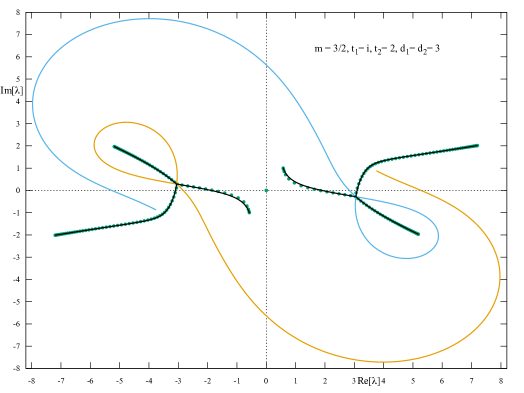
Figure 1: Plot for the non-hermitian Kitaev Chain with parameters $m=3/2$, $t_{1}=i$, $t_{2}=2$, $d_{1}=d_{2}=3$. The black lines correspond to the eigenvalues of the infinite system. The blue and yellow lines correspond to solutions for $\lambda$ of the Vieta equations, that do not correspond to actual eigenvalues of the model. The green dots correspond to eigenvalues of the finite system with $L=100$.

To illustrate this, we plot the solutions for $\lambda$ of the Vieta Eqs. (31) for the parameters $m=3/2$, $t_{1}=i$, $t_{2}=2$ and $d_{1}=d_{2}=3$ in Fig. 1. To generate the plot, we vary $\alpha$ over $0\leq\alpha<2\pi$ in steps of $2\pi/1000$. Using the solutions for $\kappa$ and $s$, we determine in which way the absolute values of $x_{i}$ are ordered. The black lines correspond to the ordering $|x_{1}|\geq|x_{2}|=|x_{3}|\geq|x_{4}|$, that is, to actual eigenvalues of the model. The blue and yellow lines correspond to the other two orderings, that do not lead to eigenvalues of the model. Finally, the green dots correspond to the eigenvalues of the finite chain with $L=100$. Fig. 1 clearly shows that the green dots closely follow the black lines, with only small deviations, caused by finite size effects. In addition, it is clear that the blue and yellow lines do not correspond to actual eigenvalues of the model. We also note the presence of the zero mode in the spectrum of the finite model. Zero modes do not correspond to solutions of the Vieta equations, as explained above.

The fact that the solutions for $x$ come in three different ‘branches’, with only one corresponding to actual eigenvalues of the model, nicely explains the presence of the ‘branching points’ that are present in the spectra of the non-hermitian Kitaev chain. We show a more intricate example of this in Sec. VII below. There, we also discuss the known stability problems of finding the eigenvalues of a large finite (non-hermitian) system.

We close this section by noting that if we know the spectrum for a given set of parameters, we in fact know the spectrum for a one-parameter set of parameters. In particular, the right hand sides of the Vieta Eqs. (31) are invariant under

$$m \rightarrow me^{i\phi} t_{s} \rightarrow t_{s}e^{i\phi} t_{d} \rightarrow t_{d}e^{i\phi} d_{1}d_{2} \rightarrow d_{1}d_{2}e^{2i\phi} \lambda \rightarrow\lambda e^{i\phi}\ ,$$ (32)

meaning that if one changes phases of the parameters in the way indicated, the whole spectrum is rigidly phase rotated. We note that this basically corresponds to multiplying the whole matrix Eq. (3) by a constant phase, which leaves the eigenvectors invariant (one can of course also rescale the spectrum in the same way).

VI Presence of the skin effect

Because we have a rather compact characterisation of the eigenvalues of the model in the thermodynamic limit we can, in principle, analyse in detail for which parameters the model has a skin effect. In solving the model in the infinite size limit, we obtained that two roots of the bulk equation are equal in absolute value, see Eq. (30). Because the roots $x_{2}$ and $x_{3}$ with $|x_{2}|=|x_{3}|$ determine the corresponding eigenvector, we find that there is no skin effect when $|x_{2}|=|x_{3}|=1$. The eigenvalues of the eigenstates that do not show a skin effect, lie on the curves of the eigenvalues in the periodic case $\lambda_{\pm}(k)$, as given by Eq. (11). We are interested in determining the parameters of the model, for which there are eigenstates that do not show the skin effect for extended ranges of $k$. We will not in general try to locate isolated points.

There is a long history of determining the location of the roots of polynomials in the complex plane and several algorithms exist to determine, say, how many roots have a negative real part, without having to determine the actual roots. Such algorithms are often used in stability analyses of various systems. For instance, the Routh–Hurwitz stability criterion Ro1877 ; Hu1895 determines if all the roots of a polynomial have negative real parts. One way to derive the criterion is to construct the sequence of Sturm polynomials associated with the polynomial under investigation St1829 .

The algorithm we focus on is tailored to determine the number of roots within, on and outside of the unit circle. This is achieved by using a conformal map, that maps the imaginary axis to the unit circle. In particular, the algorithm we use is due to Bistritz Bi2002 , but also in the case of finding the number of roots inside the unit circle, the topic has a long history, dating back a century at least Co1922 .

For a polynomial with explicit coefficients, the algorithm fully determines the number of roots of each ‘type’. We however, would like to determine the number of roots on the unit circle as a function of the parameters in the model. This is a harder problem, and although we believe we determined all cases for which there are at least two roots on the unit circle, we do not have a proof for this in the general case with complex parameters.

The starting point of the algorithm is a polynomial of degree $n$, $P_{n}(x)$, and we assume that $P_{n}(1)=1$. As long as $P_{n}(1)\neq 0$, we can always rescale $P_{n}(x)$ as necessary. If $P_{n}(1)=0$, we can factorise out the root $x=1$. From the polynomial $P_{n}(x)$, a set of polynomials $T_{i}(x)$, of degree $i$ with $i=n,n-1,\ldots,0$ is constructed. In this paper, we do not describe the actual algorithm to determine the polynomials $T_{i}(x)$, but simply state the results and refer to Bi2002 for the details.

In general, the algorithm to determine the polynomials $T_{i}(x)$ can be ‘regular’ or ‘singular’. For now, we assume that the algorithm is ‘regular’ and discuss the singular case below. We assume that we obtained the polynomials $T_{i}(x)$ explicitly.

From the polynomials $T_{i}(x)$ one forms the sequence

$$A=\{T_{n}(1),T_{n-1}(1),\ldots T_{1}(1),T_{0}(1)\}\ .$$ (33)

The algorithm to define the $T_{i}(x)$ guarantees that $T_{i}(1)$ is real for all $i$. Therefore, we can define $\nu_{n}$ as the number of sign changes in the sequence $A$. The number of zeroes of $P(x)$ inside the unit circle is then given by $\alpha_{n}=n-\nu_{n}$, while the number of zeroes of $P(x)$ outside the unit circle is given by $\gamma_{n}=\nu_{n}$.

If the polynomial $P_{n}(x)$ has one or more roots on the unit circle, the algorithm is ‘singular’. In particular, the algorithm is singular at level $s$ if $T_{s}(0)\neq 0$ and $T_{s-1}(x)\equiv 0$. In this case, the algorithm proceeds in a slightly different manner, and one obtains different polynomials $T^{\prime}_{s-1}(x),T^{\prime}_{s-2}(x),\ldots T^{\prime}_{1}(x),T^{\prime}_{0}(x)$ (which also have the property that $T^{\prime}_{i}(1)$ is real for all $i$). In this case, one defines

$$A =\{T_{n}(1),T_{n-1}(1),\ldots,T_{s}(1),T^{\prime}_{s-1}(1),T^{\prime}_{s-2}(1)\ldots T^{\prime}_{1}(1),T^{\prime}_{0}(1)\}$$ (34)

$$B =\{T_{s}(1),T^{\prime}_{s-1}(1),T^{\prime}_{s-2}(1)\ldots T^{\prime}_{1}(1),T^{\prime}_{0}(1)\}\ .$$ (35)

Again, $\nu_{n}$ is the number of sign changes in $A$, but we now also define $\nu_{s}$ as the number of sign changes in $B$. In this case, the number of zeroes inside the unit circle is $\alpha_{n}=n-\nu_{n}$, the number of zeroes on the unit circle is $\beta_{n}=2\nu_{s}-s$, while the number of zeroes outside of the unit circle is $\gamma_{n}=n-\alpha_{n}-\beta_{n}$.

For our problem, we analyse the bulk equation, which we write as follows

$$P(x)=\frac{1}{N_{2}}\bigl{(}D_{2}(1+x^{4})+x^{3}(-\lambda t_{d}-mt_{s})+x(\lambda t_{d}-mt_{s})+x^{2}(N_{2}+2mt_{s}-2D_{2})\Bigr{)}\ ,$$ (36)

with

$$N_{2} =\lambda^{2}-(m+t_{s})^{2} D_{2} =d_{1}d_{2}-t_{1}t_{2} t_{s} =t_{1}+t_{2} t_{d} =t_{1}-t_{2}\ .$$ (37)

The polynomial $P(x)$ is scaled such that $P(1)=1$.

To proceed, we note that when the system does not exhibit skin effect, the eigenvalues $\lambda$ of the open chain that we study lie on the curve given by the eigenvalues of the periodic chain. We use this information when analysing the sequences $A$ and $B$ defined above. The eigenvalues for the periodic chain are given by Eq. (11) with $0\leq k<2\pi$.

Because the solution in the periodic case satisfies the same bulk equation, we find that $x=e^{ik}$ is a root of $P(x)$ provided that we set $\lambda=\lambda_{+}(k)$. Similarly, $x=e^{-ik}$ is a root of $P(x)$ for $\lambda=\lambda_{-}(k)$. In both cases, at least one of the roots lies on the unit circle, implying that the Bistritz algorithm is singular at some level (when $\lambda$ is set to $\lambda_{\pm}(k)$). For this reason, we should analyse at which level the algorithm is singular, depending on the parameters of the model.

If we find that the algorithm is singular at level $s$, with $s$ even, we know that the number of zeroes on the unit circle, given by $\beta_{n}=2\nu_{s}-s$ is also even. This implies that there are at least two zeroes on the unit circle, because we know that there is at least one such zero. This in turn implies the absence of the skin effect. Because the product of the roots $x_{1}x_{2}x_{3}x_{4}=1$, we also know that is it not possible to have precisely three roots on the unit circle.

VI.1 Skin effect for the model with real parameters.

In the case of polynomials with complex parameters, the Bistritz algorithm becomes cumbersome, because constructing the polynomials $T_{i}(x)$ involves taking the complex conjugate. Therefore, we initially focus on the case with real parameters $m,t_{1},t_{2},d_{1},d_{2}$, but of course allow $\lambda$, and hence $N_{2}$, to be complex. In this case, we obtain the following results for the polynomials $T_{i}(x)$. For $T_{4}(x)$, we have

$$T_{4}(x) =2\Bigl{(}D_{2}\operatorname{Re}(N_{2})(1-2x^{2}+x^{4})-mt_{s}\operatorname{Re}(N_{2})(x-2x^{2}+x^{3})+it_{d}\operatorname{Im}(\lambda N_{2}^{*})(x-x^{3})\Bigr{)}/(N_{2}N_{2}^{*})+2x^{2}$$

$$T_{4}(1) =2$$ (38)

$$T_{4}(0) =2D_{2}\operatorname{Re}(N_{2})/(N_{2}N_{2}^{*})\ .$$

For $T_{3}(x)$, we have

$$T_{3}(x) =2\Bigl{(}iD_{2}\operatorname{Im}(N_{2})(1+x-x^{2}-x^{3})-imt_{s}\operatorname{Im}(N_{2})(x-x^{2})-t_{d}\operatorname{Re}(\lambda N_{2}^{*})(x+x^{2})\Bigr{)}/(N_{2}N_{2}^{*})$$

$$T_{3}(1) =-4\operatorname{Re}(\lambda N_{2}^{*})/(N_{2}N_{2}^{*})$$ (39)

$$T_{3}(0) =2iD_{2}\operatorname{Im}(N_{2})/(N_{2}N_{2}^{*})\ .$$

For $T_{2}(x)$, we have

$$T_{2}(x) =-2t_{d}\operatorname{Re}(\lambda)(1-x^{2})/(i\operatorname{Im}(N_{2}))-2x$$

$$T_{2}(1) =-2$$ (40)

$$T_{2}(0) =-2t_{d}\operatorname{Re}(\lambda)/(i\operatorname{Im}(N_{2}))\ .$$

Finally, for $T_{1}(x)$, we have

$$N_{2}N_{2}^{*}\,T_{1}(x) =2\Bigl{(}-D_{2}\operatorname{Im}(N_{2})^{2}/(t_{d}\operatorname{Re}(\lambda))+t_{d}\operatorname{Re}(\lambda N_{2}^{*})\Bigr{)}(1+x)+2imt_{s}\operatorname{Im}(N_{2})(1-x)$$

$$N_{2}N_{2}^{*}\,T_{1}(1) =-4D_{2}\operatorname{Im}(N_{2})^{2}/(t_{d}\operatorname{Re}(\lambda))+4t_{d}\operatorname{Re}(\lambda N_{2}^{*})$$ (41)

$$N_{2}N_{2}^{*}\,T_{1}(0) =-2D_{2}\operatorname{Im}(N_{2})^{2}/(t_{d}\operatorname{Re}(\lambda))+2t_{d}\operatorname{Re}(\lambda N_{2}^{*})+2imt_{s}\operatorname{Im}(N_{2})\ .$$

We do not explicitly state the constant $T_{0}$, because it is a long expression and we do not need it for our purposes.

We start by analysing under which conditions $T_{3}(x)\equiv 0$. This requires $N_{2}=N_{2}^{*}$ and $(\lambda+\lambda^{*})t_{d}=0$. The first condition $N_{2}=N_{2}^{*}$ is equivalent to $\operatorname{Re}(\lambda)=0$ or $\operatorname{Im}(\lambda)=0$. The second condition $(\lambda+\lambda^{*})t_{d}=0$ is equivalent to $\operatorname{Re}(\lambda)=0$ or $t_{d}=0$. Combined, we find that $T_{3}(x)\equiv 0$ requires that either $\operatorname{Re}(\lambda)=0$ or that $\operatorname{Im}(\lambda)=t_{d}=0$.

We remark that $\operatorname{Re}(\lambda)=0$ implies that $4d_{1}d_{2}\sin(k)^{2}+(m+(t_{1}+t_{2})\cos(k))^{2}\leq 0$, which can only occur if $d_{1}$ and $d_{2}$ have opposite signs (or when $d_{1}d_{2}=0$). On the other hand, if $\operatorname{Im}(\lambda)=0$ and $t_{d}=0$ we need $4d_{1}d_{2}\sin(k)^{2}+(m+(t_{1}+t_{2})\cos(k))^{2}\geq 0$.

Finally, we note that the explicit form of $\lambda_{\pm}(k)$ implies that for $t_{d}=0$, we have that either $\operatorname{Re}(\lambda)=0$ or $\operatorname{Im}(\lambda)=0$. Hence, for $t_{d}=0$ the algorithm is singular at level $s=4$ (we recall that we assumed that all the parameters of the model are real). This finishes the analysis of the conditions $T_{3}(x)\equiv 0$.

The other way in which we can have two roots on the unit circle is when the algorithm is singular at level 2, that is when $T_{1}(x)\equiv 0$ (and $T_{2}(0)\neq 0$). By analysing the form of $T_{1}(x)$, making use of the explicit form of the eigenvalues in the periodic case $\lambda_{\pm}(k)$, one finds that $T_{1}(x)\propto mt_{s}t_{d}$. Because $T_{2}(0)\neq 0$ for $m=0$ or $t_{s}=0$, we obtain that the algoritm is also singular when either $m=0$ or $t_{s}=0$.

condition on parameters	condition on $k$
$m=0$	$\forall k$
$t_{1}=t_{2}$	$\forall k$
$t_{2}=-t_{2}$	$\forall k$
$d_{1}d_{2}<0$	$4d_{1}d_{2}\sin(k)^{2}+(m+(t_{1}+t_{2})\cos(k))^{2}<0$

Table 1: Absence of the skin effect, in the case of real parameters

We summarise the result in table 1. For the model with real parameters, there is no skin effect when either $m=0$, or when $t_{1}=\pm t_{2}$. In addition, there is no skin effect when $\operatorname{Re}(\lambda)=0$, which occurs (over an extended range for $k$) when $4d_{1}d_{2}\sin(k)^{2}+(m+(t_{1}+t_{2})\cos(k))^{2}<0$, requiring $d_{1}d_{2}<0$ (we note that $|d_{1}d_{2}|$ should be sufficiently large in order to have $4d_{1}d_{2}\sin(k)^{2}+(m+(t_{1}+t_{2})\cos(k))^{2}<0$). We note that the eigenvalues being real ($\operatorname{Im}(\lambda)=0$) alone does not imply that the skin effect is absent. Real eigenvalues can have skin effect when $t_{1}\neq t_{2}$.

To illustrate these results, we plot the (complex) spectrum of the model for several parameters. In all the plots, we use the following colour conventions. The gray curves represent the eigenvalues of the model with periodic boundary conditions. The green dots represent the eigenvalues of the open chain of finite length with $L=100$ sites. The blue lines represent eigenvalues of the infinite open chain, corresponding to eigenstates that do have skin effect. Finally, the red lines represent eigenvalues of the infinite open chain, corresponding to eigenstates that do not have skin effect. The latter eigenvalues also correspond to eigenvalues of the periodic chain.

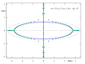
Figure 2: The eigenvalues of the model with parameters $m=2/5$, $t_{1}=2$, $t_{2}=1$, $d_{1}=-d_{2}=\sqrt{3}$. The gray lines correspond to the periodic case; the green dots correspond to the open finite chain with $L=100$; the blue (red) lines correspond eigenvalues of the open infinite chain whose eigenstates do (do not) exhibit the skin effect. The eigenvalues along the imaginary axis extent to $\lambda\approx\pm 4.4495i$.

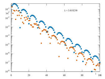
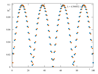
Figure 3: The amplitude of eigenstate coefficients for two states of the finite $L=100$ model with parameters $m=2/5$, $t_{1}=2$, $t_{2}=1$, $d_{1}=-d_{2}=\sqrt{3}$. The left panel corresponds to a real eigenvalue ($\lambda\approx 3.0182$) showing skin effect (note the logarithmic scale), the right panel corresponds to a purely imaginary eigenvalue ($\lambda\approx 4.3949i$) without skin effect.

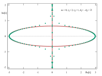
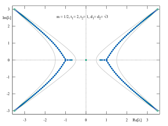
Figure 4: The eigenvalues for two sets of parameters. The colour coding is the same as in Fig. 2. The parameters for the left panel are $m=0$, $t_{1}=2$, $t_{2}=1$, $d_{1}=-d_{2}=\sqrt{3}$; in this case, none of the eigenstates exhibit skin effect, thus the red and gray curves coincide. The purely imaginary eigenvalues extend to $\pm(1+2\sqrt{3})i\approx\pm 4.4641i$. We cut off the figure for clarity. The parameters for the right panel are $m=1/2$, $t_{1}=2$, $t_{2}=1$, $d_{1}=d_{2}=\sqrt{3}$; in this case, all the eigenstate exhibit skin effect. We note that in this case, there is zero-mode.

In Fig. 2, we plot the eigenvalues of the system with parameters $m=2/5$, $t_{1}=2$, $t_{2}=1$, $d_{1}=-d_{2}=\sqrt{3}$. The figure clearly shows that for these parameters (which do no fall in one of the classes $m=0$ or $t_{1}=\pm t_{2}$), some of the eigenstates of the infinite open chain do show skin effect, while others do not. The eigenvalues that are purely imaginary do not show skin effect, while those that lie in the region bounded by the two ovals (corresponding to eigenvalues of the periodic case) do show skin effect. Interestingly, there are real (non-zero) eigenvalues that correspond to states that do exhibit skin effect. In the hermitian case, non-zero (and necessarily real) eigenvalues do not exhibit skin effect. In Fig. 3, we plot the absolute value of the eigenstate coefficients as a function of position for two eigenvalues of the finite chain namely $\lambda\approx 3.0182$ in the left panel (real eigenvalue with skin effect, using a logarithmic scale) and $\lambda\approx 4.3949i$ in the right panel (purely imaginary eigenvalue without skin effect).

Depending on the parameters, it can also happen that either all the eigenstates of the model have skin effect (this is the generic case), or none of the eigenstates have skin effect. In Fig. 4, we show an example of either case.

VI.2 Skin effect for the model with complex parameters.

In this section, we consider the model with complex parameters, generalising the results of the previous section. As in the case of real parameters, we do not try to find all isolated points for which the eigenstates do not show a skin effect (this could occur when the curves describing the eigenvalues in the periodic case, i.e., $\lambda_{\pm}(k)$, self intersect).

In the previous section, we obtained that $m=0$, $t_{1}=t_{2}$ and $t_{1}=-t_{2}$ are three different sufficient conditions implying that there is no skin effect for all the eigenstates in the case of real parameters. We now argue that these three conditions remain sufficient in the case of complex parameters.

To show this, we consider the Vieta Eqs. (31), and solve them for $\kappa$, $s$ and $\lambda$ under the conditions $m=0$, $t_{1}=-t_{2}$ or $t_{1}=t_{2}$. When either $m=0$ or $t_{1}=-t_{2}$, we find that there are solutions with $\kappa=\pm i$. When $t_{1}=t_{2}$, there are solutions with $\kappa=\pm 1$. Because in all these cases, $|\kappa|=1$ we find that the ordering of the roots satisfies $|x_{1}|\geq|x_{2}|=|x_{3}|\geq|x_{4}|$, which shows that the obtained solutions correspond to actual eigenvalues of the model. Because $|\kappa|=1$, the eigenstates do not exhibit a skin effect. Indeed, in these cases the form of $\lambda$ as obtained from the Vieta equations corresponds to the eigenvalues of the periodic case, $\lambda_{\pm}(k)$, which has to be true in the absence of the skin effect.

We continue by generalising the results for real parameters, that originated from the condition $T_{3}(x)\equiv 0$. In order to do this, we need the form of the Bistritz polynomials for complex parameters. Because these are quite involved, we state them in Appendix A. In particular, we need $T_{3}(x)$ as given in Eq. (A).

We find that the condition $T_{3}(x)\equiv 0$ is equivalent to the following conditions on the parameters in the model

$$\operatorname{Im}(D_{2}N_{2}^{*}) =0 \operatorname{Im}(mt_{s}N_{2}^{*}) =0 \operatorname{Re}(\lambda t_{d}N_{2}^{*}) =0\ .$$ (42)

Let us denote the argument of $m$, $t_{s}$, etc. by $\phi_{m}$, $\phi_{t_{s}}$, etc., then the conditions above reduce to

$$\phi_{D_{2}} =\phi_{N_{2}}\bmod\pi \phi_{m}+\phi_{t_{s}} =\phi_{N_{2}}\bmod\pi \phi_{\lambda}+\phi_{t_{d}} =\phi_{N_{2}}+\pi/2\bmod\pi\ .$$ (43)

We note that $N_{2}$ is not independent of the parameters. Making use of the explicit form of $\lambda$ in the periodic case, we obtain

$$N_{2}=\lambda^{2}-(m+t_{s})^{2}=2mt_{s}\bigl{(}\cos(k)-1\bigr{)}+4D_{2}\sin(k)^{2}+2i\lambda t_{d}\sin(k)\ ,$$ (44)

which implies that the relations Eq. (43) are satisfied, provided that $\phi_{D_{2}}=\phi_{m}+\phi_{t_{s}}=\phi_{\lambda}+\phi_{t_{d}}+\pi/2\bmod\pi$. To continue, we assume that $\phi_{m}=\phi_{D_{2}}-\phi_{t_{s}}\bmod\pi$ and $\phi_{\lambda}=\phi_{D_{2}}-\phi_{t_{d}}-\pi/2\bmod\pi$. Then, the condition $T_{3}(x)\equiv 0$ reduces to

$$|\lambda|^{2}\sin(\phi_{D_{2}}-2\phi_{t_{d}})+(|m|^{2}-|t_{s}|^{2})\sin(\phi_{D_{2}}-2\phi_{t_{s}})=0\ .$$ (45)

Because we are interested in extended regions in $k$ for which there is no skin effect, we obtain that $\phi_{t_{d}}=\phi_{t_{s}}\bmod\pi/2$, and $\phi_{D_{2}}=2\phi_{t_{s}}=2\phi_{t_{d}}\bmod\pi$. Because of the relation $D_{2}=d_{1}d_{2}-t_{1}t_{2}$, we can replace the relation $\phi_{D_{2}}=2\phi_{t_{s}}\bmod\pi$ by $\phi_{d_{1}d_{2}}=2\phi_{t_{s}}\bmod\pi$, where $\phi_{d_{1}d_{2}}$ is the phase of $d_{1}d_{2}$.

Combined, we find the following conditions, which are necessary in order that the Bistritz algorithm is singular at level 4

$$\phi_{m} =\phi_{t_{s}}\bmod\pi \phi_{\lambda} =\phi_{t_{d}}+\pi/2\bmod\pi \phi_{d_{1}d_{2}} =2\phi_{t_{s}}\bmod\pi \phi_{t_{d}} =\phi_{t_{s}}\bmod\pi/2\ .$$ (46)

We still need to check when these conditions are compatible with the explicit form of the eigenvalues in the periodic case, $\lambda_{\pm}(k)$ as given in Eq. (11). By analysing the form of $\lambda_{\pm}(k)$, taking the phase relations into account, one finds that the form of $d_{1}d_{2}$ is crucial. Generically, we write $d_{1}d_{2}=|d_{1}d_{2}|e^{i\phi_{d_{1}d_{2}}}$. In Table 2, we state the conditions such that the eigenstates do not show a skin effect (due to $T_{3}(x)\equiv 0$), resulting from this analysis. We note that the third line also follows from the analysis of the case with real parameters in the previous subsection and the result that phase-rotating the parameters of the model according to Eq. (32) leads to a rigid phase rotation of the spectrum.

$t_{s}$	$t_{d}$	$m$	$d_{1}d_{2}$	$\lambda$	absence skin effect
$|t_{s}|e^{i\phi_{t_{s}}}$	$\pm i|t_{d}|e^{i\phi_{t_{s}}}$	$\pm|m|e^{i\phi_{t_{s}}}$	$+|d_{1}d_{2}|e^{2i\phi_{t_{s}}}$	$\pm|\lambda|e^{i\phi_{t_{s}}}$	$\forall k$
$|t_{s}|e^{i\phi_{t_{s}}}$	$\pm i|t_{d}|e^{i\phi_{t_{s}}}$	$\pm|m|e^{i\phi_{t_{s}}}$	$-|d_{1}d_{2}|e^{2i\phi_{t_{s}}}$	$\pm|\lambda|e^{i\phi_{t_{s}}}$	$-4|d_{1}d_{2}|\sin(k)^{2}+(\pm|m|+|t_{s}|\cos(k))^{2}>0$
$|t_{s}|e^{i\phi_{t_{s}}}$	$\pm|t_{d}|e^{i\phi_{t_{s}}}$	$\pm|m|e^{i\phi_{t_{s}}}$	$-|d_{1}d_{2}|e^{2i\phi_{t_{s}}}$	$\pm i|\lambda|e^{i\phi_{t_{s}}}$	$-4|d_{1}d_{2}|\sin(k)^{2}+(\pm|m|+|t_{s}|\cos(k))^{2}<0$

Table 2: Sufficient conditions for absence of the skin effect (due to $T_{3}(x)\equiv 0$).

An obvious check on these results is to consider the hermitian case, with $N_{2},\lambda,m,D_{2},t_{s}$ all real, and $t_{d}$ purely imaginary. In this case, one finds that indeed $T_{3}(x)\equiv 0$ implying that the Bistritz algorithm is singular at level 4. This in turn implies that the eigenstates do not have a skin effect, as expected.

The other way in which the skin effect is absent, is when $T_{1}(x)\equiv 0$. The coefficients of the polynomial $T_{1}(x)$ are much more involved, see Eq. (52). We therefore do not attempt to fully characterise for which (complex) parameters of the model one has $T_{1}(x)\equiv 0$. However, above we argued based on the Vieta equations that for either $m=0$, $t_{s}=0$, or $t_{d}=0$, the eigenstates do not show a skin effect. This means that under these conditions $T_{1}(x)\equiv 0$ even when the other parameters are complex. We are interested in generic results, that is, extended regions of the curves of eigenvalues, for which the skin effect is absent. We believe that the conditions provided, exhaust all these cases. The argument in favour of this statement is that we need that $T_{1}(x)\equiv 0$ with $\lambda=\lambda_{\pm}(k)$, for an extended range of $k$. Due to the form of $\lambda_{\pm}(k)$, this only seems possible when the various terms of $\lambda_{\pm}(k)$ have the same argument, or when one or more of the parameters is zero.

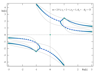
Figure 5: The eigenvalues for a set including complex parameters, namely $m=2i/5$, $t_{1}=2+i$, $t_{2}=1$, $d_{1}=-d_{2}=\sqrt{3}$. The colour coding is the same as in Fig. 2.

We conclude this section with a characteristic example of the eigenvalues for a case with complex parameters, namely $m=2i/5$, $t_{1}=2+i$, $t_{2}=1$, $d_{1}=-d_{2}=\sqrt{3}$ as shown in Fig. 5. In this generic case, all the generic eigenstates exhibit the skin effect. As expected, the spectrum is significantly more complex compared to the cases we showed with real parameters. We note that the gray curves of the eigenvalues $\lambda_{\pm}(k)$ in the periodic case intersect themselves. The eigenvalues of the open chain in the large system size limit (given by the blue curves) cross these intersection points. This means that the eigenstates corresponding to these (six) special eigenvalues do not have a skin effect. We checked this behaviour explicitly, by solving the bulk Eq. (8), confirming that two solutions for $x$ indeed have modulus one. In addition, we checked that the Bistritz polynomial $T_{1}(x)\equiv 0$ for the given parameters and the eigenvalue $\lambda$.

VII Discussion

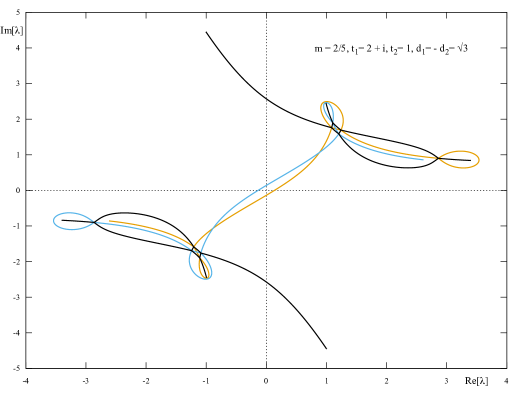
Figure 6: Solutions for $\lambda$ of the Vieta equations, for $m=2/5$, $t_{1}=2+i$, $t_{2}=1$, $d_{1}=-d_{2}=\sqrt{3}$. Only the black lines correspond to actual eigenvalues. For the blue and dark-yellow lines, the solutions $x_{i}$ of the bulk equation correspond to one of the branches that do not correspond to actual eigenvalues.

We studied the non-hermitian Kitaev chain for general complex parameters, pushing analytical methods as far as possible. We now discuss our results, by means of an example. We use the chain with parameters $m=2/5$, $t_{1}=2+i$, $t_{2}=1$, $d_{1}=-d_{2}=\sqrt{3}$ for this purpose. One of the main results we obtained in this paper, is the characterisation of the eigenvalues of the infinite size system, in terms of three Vieta Eqs. (31), for $\lambda$ which we repeat here for convenience,

$$\bigl{(}\kappa+\frac{1}{\kappa}\bigr{)}\bigl{[}(s+\frac{1}{s})+2\cos\alpha\bigr{]}=\frac{2m(t_{1}+t_{2})}{d_{1}d_{2}-t_{1}t_{2}}$$

$$\bigl{(}\kappa-\frac{1}{\kappa}\bigr{)}\bigl{[}(s+\frac{1}{s})-2\cos\alpha\bigr{]}=\frac{2\lambda(t_{1}-t_{2})}{d_{1}d_{2}-t_{1}t_{2}}$$

$$(\kappa+\frac{1}{\kappa})^{2}+2\cos\alpha(s+\frac{1}{s})=\frac{\lambda^{2}-m^{2}-(t_{1}+t_{2})^{2}}{d_{1}d_{2}-t_{1}t_{2}}\ .$$ (47)

where $\kappa$ and $s$ are in general complex. The eigenvalue curves $\lambda$ are obtained by varying $0\leq\alpha<2\pi$, but only those $\lambda$ that correspond to solutions that satisfy $1/|s|\leq|\kappa|^{2}\leq|s|$ are actual eigenvalues of the model as explained in Sec. V.

In Fig. 6, we show the eigenvalues of the model with parameters $m=2/5$, $t_{1}=2+i$, $t_{2}=1$, $d_{1}=-d_{2}=\sqrt{3}$ as an illustration. The actual eigenvalues (the black lines) form a rather intricate pattern, which can be explained in terms of the three different branches of solutions of the Vieta equations. Fig. 6 also shows the other two branches (the blue and yellow lines), that do not correspond to eigenvalues of the model. It is interesting to note the regions where the black lines ‘intersect’. Here, the eigenvalues do not cross, nor do they repel, but form a rhombic structure.

The reason why having a concise characterisation for the infinite system size model is useful, is that (as is well known) obtaining the eigenvalues for large, non-hermitian systems showing skin-effect is numerically unstable. We illustrate this using the same example, by plotting the eigenvalues, as obtained using machine precision diagonalisation for system sizes $L=100$, $L=200$, $L=400$ and $L=800$. The results are shown in Fig. 7 as the green dots, together with the infinite system size results.

We clearly see that for sizes $L=100$ and $L=200$, the eigenvalues closely follow the black lines corresponding to the infinite size model, with only minor difference due to the finite size effects. However, already for $L=400$, there is a region where the finite size eigenvalues deviate substantially from curves for infinite size. Moreover, the ‘eigenvalues’ in this region do not satisfy particle-hole symmetry (dictating that if $\lambda$ is an eigenvalue, so is $-\lambda$), which clearly indicates that these values obtained by the diagonalisation algorithm are incorrect. For $L=800$, the situation gets worse. In principle, one can obtain the correct eigenvalues even for these larger system sizes, if one uses a diagonalisation algorithm employing higher precision arithmetic, but in practise, this will be much slower that obtaining the infinite system size results.

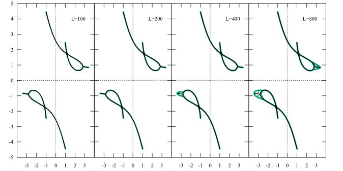
Figure 7: Finite size eigenvalues for the model with parameters $m=2/5$, $t_{1}=2+i$, $t_{2}=1$, $d_{1}=-d_{2}=\sqrt{3}$. The black lines correspond to actual eigenvalues in the limit $L\rightarrow\infty$. The different panels show the numerically obtained eigenvalues (using machine precision) for the sizes $L=100$, $L=200$, $L=400$ and $L=800$, showing the instability of the algorithm (green dots).

By making use of the exact solution, we studied the presence of the skin effect. There exist methods to determine if a model exhibits skin effect for a given set of parameters. Here, we also characterise which eigenvalues have eigenstates showing the skin effect, or rather, which ones do not show skin effect. We formulated this condition in terms of the solutions for $x$ of the bulk Eq. (7), namely if at least two (out of the four) solutions lie on the unit circle, the corresponding eigenstate does not have a skin effect. We used the Bistritz algorithm to determine under which conditions there are states without skin effect, and to which eigenvalues these correspond. We provided a full characterisation for the non-hermitian model with real parameters. For the general model with complex parameters we provide sufficient conditions for the absence of the skin effect, which we believe are also necessary.

Finally, we studied under which conditions, the non-hermitian Kitaev chain has a zero mode (for the hermitian Kitaev chain, this corresponds to the region where the model is in the topological phase). It turns out that this region has perhaps a more complicated structure than one would expect. Namely, the model has a zero mode when the following condition is satisfied,

$$|\operatorname{Im}(\arccos\bigl{(}-\frac{m}{2\sqrt{t_{1}t_{2}-d_{1}d_{2}}}\bigr{)})|<|\operatorname{Im}(\arccos\bigl{(}\frac{t_{1}+t_{2}}{2\sqrt{t_{1}t_{2}-d_{1}d_{2}}}\bigr{)})|\ .$$ (48)

At the boundary of this region, the model is gapless, but even outside of this region, the model can be gapless. In the hermitian version of the model, this would correspond to a metallic, gapless system.

Despite the fact that non-hermitian one-dimensional models have been studied in great detail, it would be interesting to apply the method to characterise the eigenvalues in the thermodynamic limit to other, more complicated systems. Here, one can think of models with larger unit cells and models with longer range interactions. Obviously, this will lead to higher order equations and more complicated expressions.

Appendix A Bistritz polynomials for complex parameters

In this appendix, we give the Bistritz polynomials $T_{i}(x)$ (with $4\geq i\geq 1$) in the general case, that is for complex parameters. For details on the Bistritz algorithm, we refer to Bi2002 .

The polynomial $T_{4}(x)$ reads

$$T_{4}(x) =2\Bigl{(}\operatorname{Re}(D_{2}N_{2}^{*})(1-2x^{2}+x^{4})+i\operatorname{Im}(\lambda t_{d}N_{2}^{*})(x-x^{3})-\operatorname{Re}(mt_{s}N_{2}^{*})(x-2x^{2}+x^{3})\Bigr{)}/(N_{2}N_{2}^{*})+2x^{2}$$

$$T_{4}(1) =2$$ (49)

$$T_{4}(0) =2\operatorname{Re}(D_{2}N_{2}^{*})/(N_{2}N_{2}^{*})\ .$$

For $T_{3}(x)$, we obtain the following expression

$$T_{3}(x) =2\Bigl{(}-i\operatorname{Im}(D_{2}N_{2}^{*})(1+x-x^{2}-x^{3})+i\operatorname{Im}(mt_{s}N_{2}^{*})(x-x^{2})-\operatorname{Re}(\lambda t_{d}N_{2}^{*})(x+x^{2})\Bigr{)}/(N_{2}N_{2}^{*})$$

$$T_{3}(1) =-4\operatorname{Re}(\lambda t_{d}N_{2}^{*})/(N_{2}N_{2}^{*})$$ (50)

$$T_{3}(0) =-2i\operatorname{Im}(D_{2}N_{2}^{*})/(N_{2}N_{2}^{*})\ .$$

$T_{2}(x)$ is given by

$$T_{2}(x) =2\Bigl{(}\operatorname{Re}(\lambda t_{d}D_{2}^{*})(1-x^{2})-i\operatorname{Im}(mt_{s}D_{2}^{*})(1-2x+x^{2})\Bigr{)}/(i\operatorname{Im}(D_{2}N_{2}^{*}))-2x$$

$$T_{2}(1) =-2$$ (51)

$$T_{2}(0) =2\Bigl{(}\operatorname{Re}(\lambda t_{d}D_{2}^{*})-i\operatorname{Im}(mt_{s}D_{2}^{*})\Bigr{)}/(i\operatorname{Im}(D_{2}N_{2}^{*}))\ .$$

Finally, $T_{1}(x)$ is given by

$$N_{2}N_{2}^{*}T_{1}(1)=2(1+x)\Bigl{[}\operatorname{Re}(\lambda t_{d}N_{2}^{*})-\frac{\operatorname{Im}(N_{2}D_{2}^{*})^{2}\operatorname{Re}(\lambda t_{d}D_{2}^{*})}{\operatorname{Re}(\lambda t_{d}D_{2}^{*})^{2}+\operatorname{Im}(mt_{s}D_{2}^{*})^{2}}\Bigr{]}$$ (52)

$$-2i(1-x)\Bigl{[}\operatorname{Im}(mt_{s}N_{2}^{*})+4\operatorname{Im}(N_{2}D_{2}^{*})+\frac{\operatorname{Im}(N_{2}D_{2}^{*})^{2}\operatorname{Im}(mt_{s}D_{2}^{*})}{\operatorname{Re}(\lambda t_{d}D_{2}^{*})^{2}+\operatorname{Im}(mt_{s}D_{2}^{*})^{2}}-4\frac{\operatorname{Im}(N_{2}D_{2}^{*})\operatorname{Re}(\lambda t_{d}D_{2}^{*})^{2}}{\operatorname{Re}(\lambda t_{d}D_{2}^{*})^{2}+\operatorname{Im}(mt_{s}D_{2}^{*})^{2}}\Bigr{]}\ ,$$

resulting in the following expression for $T_{1}(1)$,

$$T_{1}(1)=\frac{4}{N_{2}N_{2}^{*}}\Bigl{(}\operatorname{Re}(\lambda t_{d}N_{2}^{*})-\frac{\operatorname{Im}(D_{2}^{*}N_{2})^{2}\operatorname{Re}(\lambda t_{d}D_{2}^{*})}{\operatorname{Re}(\lambda t_{d}D_{2}^{*})^{2}+\operatorname{Im}(mt_{s}D_{2}^{*})^{2}}\Bigr{)}\ .$$ (53)

Though we do not need it, we give an expression for the constant $T_{0}$, in terms of $T_{2}(x)$ an $T_{1}(x)$, for completeness

$$T_{0}=2\operatorname{Re}(T_{2}(0)/T_{1}(0))T_{1}(1)-T_{2}(1)\ .$$ (54)

References

- (1) E. J. Bergholtz, J. C. Budich, F. K. Kunst, Exceptional Topology of Non-Hermitian Systems, Rev. Mod. Phys., 93, 015005 (2021).
- (2) D. Braghini, V. D. de Lima, D. Beli, M.I.N. Rosa, J.R. de F. Arruda, Non-Hermitian acoustic waveguides with periodic electroacoustic feedback, arXiv:2210.05948.
- (3) D. C. Brody, Biorthogonal quantum mechanics, J. Phys. A 47, 035305 (2014).
- (4) P. Delplace, T. Yoshida, Y. Hatsugai, Symmetry-Protected Multifold Exceptional Points and Their Topological Characterization, Phys. Rev. Lett. 127, 186602 (2021).
- (5) E. Edvardsson, Bulk-boundary correspondence and biorthogonality in nonHermitian systems, PhD thesis, Stockholm University (2022).
- (6) E. Edvardsson, F. K. Kunst, E. J. Bergholtz, Non-Hermitian extensions of higher-order topological phases and their biorthogonal bulk-boundary correspondence, Phys. Rev. B 99, 081302(R) (2019).
- (7) Z. Gong, Y. Ashida, K. Kawabata, K. Takasan, S. Higashikawa, M. Ueda, Topological phases of non-Hermitian systems, Phys. Rev. X 8, 031079 (2018).
- (8) K. Kawabata, T. Bessho, M. Sato, Classification of exceptional points and non-Hermitian topological semimetals, Phys. Rev. Lett. 123, 066405 (2019).
- (9) K. Kawabata, K. Shiozaki, M. Ueda, M. Sato, Symmetry and topology in non-Hermitian physics, Phys. Rev. X, 9, 041015 (2019).
- (10) R. Koch, J. C. Budich, Bulk-boundary correspondence in non-Hermitian systems: Stability analysis for generalized boundary conditions, Eur. Phys. J. D 74, 70 (2020).
- (11) F. K. Kunst, V. Dwivedi, Non-Hermitian systems and topology: A transfer-matrix perspective, Phys. Rev. B 99, 245116 (2019).
- (12) F. K. Kunst, E. Edvardsson, J. C. Budich, E. J. Bergholtz, Biorthogonal bulk-boundary correspondence in non-Hermitian systems, Phys. Rev. Lett. 121, 026808 (2018).
- (13) I. Mandal, E. J. Bergholtz, Symmetry and Higher-Order Exceptional Points, Phys. Rev. Lett. 127, 186601 (2021).
- (14) V. M. Martinez Alvarez, J. E. Barrios Vargas, L. E. F. Foa Torres, Non-Hermitian robust edge states in one dimension: Anomalous localization and eigenspace condensation at exceptional points, Phys. Rev. B 97, 121401(R) (2018).
- (15) J. Larson, S. Qvarfort, Exceptional points and exponential sensitivity for periodically driven Lindblad equations, Open Systems & Information Dynamics, 30, 2350008 (2023).
- (16) T. E. Lee, Anomalous edge state in a non-Hermitian lattice, Phys. Rev. Lett, 116, 133903 (2016).
- (17) C. H. Lee, L. Li, J. Gong, Hybrid higher-order skin-topological modes in nonreciprocal systems, Phys. Rev. Lett. 123, 016805 (2019).
- (18) D. Leykam, K. Y. Bliokh, C. Huang, Y. D. Chong, F. Nori, Edge modes, degeneracies, and topological numbers in non-Hermitian systems, Phys. Rev. Lett. 118, 040401 (2017).
- (19) J. Li, Y.-C. Wang, L.-W. Duan, Q.-H. Chen, The PT-symmetric quantum Rabi model: Solutions and exceptional points, arXiv:2402.09749.
- (20) L. Li, Y. Wei, G. Wu, Y. Ruan, S. Chen, C.H. Lee, Z. Ni, Exact Solutions Disentangle Higher-Order Topology in 2D Non-Hermitian Lattices, arXiv:2410.15763.
- (21) R. Lin, L. Li, Topologically compatible non-Hermitian skin effect, Phys. Rev. B 109, 155137 (2024).
- (22) R. Lin, T .Tai, M. Yang, L. Li, C.H. Lee, Topological Non-Hermitian skin effect, Front. Phys. 18, 53605 (2023).
- (23) CC. Liu, LH. Li, J. An, Topological Invariant for Multi-Band Non-hermitian Systems with Chiral Symmetry, Phys. Rev. B 107, 245107 (2023).
- (24) A. Maddi, Y. Auregan, G. Penelet, V. Pagneux, V. Achilleos, Exact analogue of the Hatano-Nelson model in 1D continuous nonreciprocal systems, Phys. Rev. Research 6, L012061 (2024).
- (25) P. Molignini, O. Arandes, E.J. Bergholtz, Anomalous Skin Effects in Disordered Systems with a Single non-Hermitian Impurity, Phys. Rev. Research 5, 033058 (2023).
- (26) R. Nehra, D. Roy, Anomalous dynamical response of non-Hermitian topological phases, Phys. Rev. B 109, 094311 (2024).
- (27) N. Okuma, K. Kawabata, K. Shiozaki, M. Sato, Topological origin of non-Hermitian skin effects, Phys. Rev. Lett., 124, 086801 (2020).
- (28) C. Ortega-Taberner, M. Hermanns, From Hermitian critical to non-Hermitian point-gapped phases, Phys. Rev. B 107, 235112 (2023).
- (29) R. Nehra, D. Roy, Topology of multipartite non-Hermitian one-dimensional systems, Phys. Rev. B 105, 195407 (2022).
- (30) S.M. Rafi-Ul-Islam, Z.B. Siu, M.S.H. Razo, M.B.A. Jalil, Dynamic Manipulation of Non-Hermitian Skin Effect through Frequency in Topolectrical Circuits, arXiv:2410.16914.
- (31) L. Rødland, C. Ortega-Taberner, M. Agarwal, M. Hermanns, Disorder and non-Hermiticity in Kitaev spin liquids with a Majorana Fermi surface, Phys. Rev. B 109, 155162 (2024).
- (32) S. Sarkar, F. Ciccarello, A. Carollo, A. Bayat, Critical non-Hermitian topology induced quantum sensing, New J. Phys. 26 073010 (2024).
- (33) H. Shen, B. Zhen, L. Fu, Topological band theory for non-Hermitian Hamiltonians, Phys. Rev. Lett. 120, 146402 (2018).
- (34) M. Stålhammar, E. J. Bergholtz, Classification of exceptional nodal topologies protected by PT symmetry, Phys. Rev. B 104, L201104 (2021).
- (35) V. M. Vyas, D. Roy, Topological aspects of periodically driven non-Hermitian Su-Schrieffer-Heeger model, Phys. Rev. B 103, 075441 (2021).
- (36) F. Yang, E.J. Bergholtz, Anatomy of Higher-Order Non-Hermitian Skin and Boundary Modes, arXiv:2405.03750.
- (37) K. Yang, I. Mandal, Enhanced eigenvector sensitivity and algebraic classification of sublattice-symmetric exceptional points, Phys. Rev. B 107, 144304 (2023).
- (38) F. Yang, P. Molignini, E.J. Bergholtz, Dissipative Boundary State Preparation, Phys. Rev. Research 5, 043229 (2023).
- (39) S. Yao, Z. Wang, Edge States and Topological Invariants of Non-Hermitian Systems, Phys. Rev. Lett. 121, 086803 (2018).
- (40) T. Yoshida, R. Peters, N. Kawakami, Y. Hatsugai, Symmetry-protected exceptional rings in two-dimensional correlated systems with chiral symmetry, Phys. Rev. B 99, 121101(R) (2019).
- (41) L. Xiao, T. Deng, K. Wang, G. Zhu, Z. Wang, W. Yi, P. Xue, Non-Hermitian bulk-boundary correspondence in quantum dynamics, Nat. Phys. 16, 761 (2020).
- (42) Y. Xiong, Why does bulk boundary correspondence fail in some non-Hermitian topological models, J. Phys. Commun. 2, 035043 (2018).
- (43) M. Zelenayova, E.J. Bergholtz, Non-Hermitian extended midgap states and bound states in the continuum, Appl. Phys. Lett. 124, 041105 (2024).
- (44) X. Zhang, X. Song, S. Zhang, T. Zhang, Y. Liao, X. Cai, J. Li, Solvable non-Hermitian skin effects and realspace exceptional points: non-Hermitian generalized Bloch theorem, J. Phys. A: Math. Theor. 57 125001 (2024).
- (45) H. Zhou, J. Y. Lee, Periodic table for topological bands with non-Hermitian symmetries, Phys. Rev. B 99, 235112 (2019).
- (46) L. Herviou, J. H. Bardarson, N. Regnault, Defining a bulk-edge correspondence for non-Hermitian Hamiltonians via singular-value decomposition, Phys. Rev. A 99, 052118 (2019).
- (47) S. Longhi, Probing non-Hermitian skin effect and non-Bloch phase transitions, Phys. Rev. Research 1, 023013 (2019).
- (48) C. H. Lee, R. Thomale, Anatomy of skin modes and topology in non-Hermitian systems, Phys. Rev. B 99, 201103(R), (2019).
- (49) T. Liu, Y-R. Zhang, Q. Ai, Z. Gong, K. Kawabata, M. Ueda, F. Nori, Second-Order Topological Phases in Non-Hermitian Systems, Phys. Rev. Lett. 122, 076801 (2019).
- (50) C. Fleckenstein, A. Zorzato, D. Varjas, E. J. Bergholtz, J. H. Bardarson, A. Tiwari, Non-Hermitian topology in monitored quantum circuits, arXiv:2201.05341.
- (51) H.-G. Zirnstein, G. Refael, B. Rosenow, Bulk-Boundary Correspondence for Non-Hermitian Hamiltonians via Green Functions, Phys. Rev. Lett. 126, 216407 (2021).
- (52) D. S. Borgnia, A. J. Kruchkov, R.-J. Slager, Non-Hermitian Boundary Modes and Topology, Phys. Rev. Lett. 124, 056802 (2020).
- (53) K. Yokomizo, S. Murakami, Non-Bloch Band Theory of Non-Hermitian Systems, Phys. Rev. Lett. 123, 066404 (2019).
- (54) K. Yang, S. C. Morampudi, E. J. Bergholtz, Exceptional Spin Liquids from Couplings to the Environment, Phys. Rev. Lett. 126, 077201 (2021).
- (55) E. Edvardsson, F. K. Kunst, T. Yoshida, E. J. Bergholtz, Phase transitions and generalized biorthogonal polarization in non-Hermitian systems, Phys. Rev. Research 2, 043046 (2020).
- (56) H. Schomerus, Nonreciprocal response theory of non-Hermitian mechanical metamaterials: Response phase transition from the skin effect of zero modes, Phys. Rev. Research 2, 013058 (2020).
- (57) W. Brzezicki, T. Hyart, Hidden Chern number in one-dimensional non-Hermitian chiral-symmetric systems, Phys. Rev. B 100, 161105(R) (2019).
- (58) E. Edvardsson, E. Ardonne, Sensitivity of non-Hermitian systems, Phys. Rev. B, 106, 115107 (2022).
- (59) A.Y. Kitaev, Unpaired Majorana fermions in quantum wires, Phys.-Usp. 44, 131 (2001).
- (60) J. Alicea, New directions in the pursuit of Majorana fermions in solid state systems, Rep. Prog. Phys. 75 076501 (2012).
- (61) C. Yuce, Majorana edge modes with gain and loss, Phys. Rev. A 93, 062130 (2016).
- (62) M. Klett, H. Cartarius, D. Dast, J. Main, G. Wunner, Relation between -symmetry breaking and topologically nontrivial phases in the Su-Schrieffer-Heeger and Kitaev models, Phys. Rev. A 95, 053626 (2017).
- (63) C. Li, X.Z. Zhang, G. Zhang, Z. Song, Topological phases in a Kitaev chain with imbalanced pairing, Phys. Rev. B 97, 115436 (2018).
- (64) C. Li, L. Jin, Z. Song, Coalescing Majorana edge modes in non-Hermitian -symmetric Kitaev chain, Sci. Rep. 10, 6807 (2020).
- (65) K. Kawabata, Y. Ashida, H. Katsura, M. Ueda, Parity-time-symmetric topological superconductor, Phys. Rev. B 98, 085116 (2018).
- (66) S. Lieu, Non-Hermitian Majorana modes protect degenerate steady states, Phys. Rev. B 100, 085110 (2019).
- (67) X.M. Yang, Z. Song, Resonant generation of a -wave Cooper pair in a non-Hermitian Kitaev chain at the exceptional point, Phys. Rev. A 102, 022219 (2020).
- (68) X.-M. Zhao, C.-X Guo, S.-P. Kou, L. Zhuang, W.-M. Liu, Defective Majorana zero modes in non-Hermitian Kitaev chain, Phys. Rev. B 104, 205131 (2021).
- (69) T. Sakaguchi, H. Nishijima, Y. Takane, Bulk-Boundary Correspondence and Boundary Zero Modes in a Non-Hermitian Kitaev Chain Model, J. Phys. Soc. Jpn. 91, 124711 (2022).
- (70) S. Sayyad, J.L. Lado, Topological phase diagrams of exactly solvable non-Hermitian interacting Kitaev chains, Phys. Rev. Research 5, L022046 (2023).
- (71) Y.B. Shi, Z. Song, Fixed lines in a non-Hermitian Kitaev chain with spatially balanced pairing processes, Phys. Rev. B 108, 125121 (2023).
- (72) B. Li, H.-R. Wang, F. Song, Z. Wang, Non-Bloch dynamics and topology in a classical nonequilibrium process, Phys. Rev. B 109, L201121 (2024).
- (73) S. Rahul, N. Roy, R.R. Kumar, Y.R. Kartik, S. Sarkar, Unconventional quantum criticality in a non‑Hermitian extended Kitaev chain, Sci. Rep. 13, 12121 (2023).
- (74) L. Zhou, Entanglement Phase Transitions in Non-Hermitian Kitaev Chains, Entropy 26, 272 (2024).
- (75) D. Mondal, T. Nag, Persistent anomaly in dynamical quantum phase transition in long-range non-Hermitian p-wave Kitaev chain, Eur. Phys. J. B 97, 59 (2024).
- (76) K. Fukui, Y. Kato, Y. Motome, Magnetic field effects on the Kitaev model coupled to environment, Phys. Rev. B 110, 024429 (2024).
- (77) D.M. Pino, Y. Meir, R. Aguado, Thermodynamics of Non-Hermitian Josephson junctions with exceptional points, arXiv:2405.02387.
- (78) J. Cayao, R. Aguado, Non-Hermitian minimal Kitaev chains, arXiv:2406.18974.
- (79) S. Li, M. Liu, Y. Zhang, R. Tian, M. Arzamasovs, B. Liu, Anomalous symmetry-protected blockade of the skin effect in one-dimensional non-Hermitian lattice systems, Phys. Rev. A 110, 042208 (2024).
- (80) E. Lieb, T. Schultz, D. Mattis, Two soluble models of an antiferromagnetic chain, Ann. Phys. 16, 407 (1961).
- (81) I. Mahyaeh, E. Ardonne Zero modes of the Kitaev chain with phase-gradients and longer range couplings, J. Phys. Commun. 2, 045010 (2018).
- (82) P.L. Chebyshev, Théorie des mécanismes connus sous le nom de parallélogrammes, Imprimerie de l’Académie impériale des sciences (1853).
- (83) N. Hatano, D. R. Nelson, Localization Transitions in Non-Hermitian Quantum Mechanics, Phys. Rev. Lett. 77, 570 (1996).
- (84) N. Hatano, D. R. Nelson, Vortex pinning and non-Hermitian quantum mechanics, Phys. Rev. B 56, 8651 (1997).
- (85) N. Hatano, D. R. Nelson, Non-Hermitian delocalization and eigenfunctions, Phys. Rev. B 58, 8384 (1998).
- (86) F. Viète, Opera Mathematica, published by Franciscus van Schooten with commentaries, Leiden, 1646. Reprint by Georg Olms Verlag, Hildesheim, New York (1970).
- (87) E.J. Routh, A treatise on the stability of a given state of motion, particularly steady motion, London, Macmillan and co. (1877).
- (88) A. Hurwitz, Ueber die Bedingungen, unter welchen eine Gleichung nur Wurzeln mit negativen reellen Theilen besitzt, Math. Ann. 46, 273 (1895).
- (89) P.C. Sturm, Mémoire sur la résolution des équations numériques, Bulletin des Sciences de Férussac. 11, 419 (1829); Collected Works of Charles François Sturm, Birkhäuser Basel (2009) .
- (90) Y. Bistritz, Zero Location of Polynomials With Respect to the Unit-Circle Unhampered by Nonessential Singularities, IEEE Transactions on Circuits and Systems I: Fundamental Theory and Applications, 49, 305 (2002).
- (91) A. Cohn, Über die Anzahl der Wurzeln einer algebraischen Gleichung in einem Kreise, Mathematische Zeitschrift 14, 110 (1922).