Kolmogorov Modes and Linear Response of Jump-Diffusion Models:
Applications to Stochastic Excitation of the ENSO Recharge Oscillator
Abstract
We introduce a generalization of linear response theory for mixed jump-diffusion models, combining both Gaussian and Lévy noise forcings that interact with the nonlinear dynamics. This class of models covers a broad range of stochastic chaos and complexity for which the jump-diffusion processes are a powerful tool to parameterize the missing physics or effects of the unresolved scales onto the resolved ones.
By generalizing concepts such as Kolmogorov operators and Green’s functions to this context, we derive fluctuation-dissipation relationships for such models. The system response can then be interpreted in terms of contributions from the eigenmodes of the Kolmogorov operator (Kolmogorov modes) decomposing the time-lagged correlation functions of the unperturbed dynamics. The underlying formulas offer a fresh look on the intimate relationships between the system’s natural variability and its forced variability.
We apply our theory to a paradigmatic El Niño-Southern Oscillation (ENSO) subject to state-dependent jumps and additive white noise parameterizing intermittent and nonlinear feedback mechanisms, key factors in the actual ENSO phenomenon. Such stochastic parameterizations are shown to produce stochastic chaos with an enriched time-variability. The Kolmogorov modes encoding the latter are then computed, and our Green’s functions formulas are shown to achieve a remarkable accuracy to predict the system’s response to perturbations.
This work enriches Hasselmann’s program by providing a more comprehensive approach to climate modeling and prediction, allowing for accounting the effects of both continuous and discontinuous stochastic forcing. Our results have implications for understanding climate sensitivity, detection and attributing climate change, and assessing the risk of climate tipping points.
pacs:
05.45.-a, 89.75.-kI Introduction
Two key tasks in understanding complex systems consist of analyzing their modes of spatial-temporal variability and assessing their sensitivity to perturbations. Unperturbed variability reveals the underlying (nonlinear) processes driving the system’s dynamics across various scales. Sensitivity to perturbations, on the other hand, is linked to the strength of the system’s internal feedbacks. Critical transitions occur when positive feedbacks overwhelm negative ones, making the system vulnerable to external influences.
The fluctuation-dissipation theorem (FDT) is a fundamental principle in statistical physics that connects the response of a system to external perturbations with the fluctuations of its internal variables, for systems near thermodynamic equilibrium. The FDT roughly states that for such systems, the average response to small external perturbations can be calculated through the knowledge of suitable time-lagged correlation functions of the unperturbed statistical system Kubo1966 ; marconi2008fluctuation ; kubo2012statistical .
Beyond isolated conservative systems, linear response theory (LRT) has been (rigorously) extended to non-equilibrium systems that include chaotic systems exhibiting a strange attractor ruellegeneral1998 ; butterley2007smooth ; ruelle2009 . However, the situation is much more complex here. Indeed, the attractors of chaotic systems have typically very intricate fractal structure, making the direct link between free fluctuation statistics and response challenging as the asymptotic statistics collected on the strange attractor do not contain information about the dynamics outside it. Constructing response operators from unperturbed flow statistics becomes then computationally demanding Wang2013 ; Ni2017 ; Chandramoorthy2022 ; Ni2023 . Alternatively, carefully designed perturbed experiments (exploiting covariant Lyapunov vectors) offer a practical approach to circumvent these computational challenges LucariniSarno2011 ; gritsun2017 .
For complex systems though, it is a common practice to add a small amount of Gaussian noise to chaotic dissipative systems. This regularization technique can simplify the analysis by smoothing the attractor. Such noise can be physically justified as a representation of unresolved physical processes (stochastic parameterization palmer2005representing ; berner2017stochastic ; LucariniChekroun2023 ) or the result of eliminating fast variables majda2001mathematical .
The increased regularity due to noise significantly simplifies the analysis, overcoming challenges encountered in deterministic systems baladi2014 ; Baladi2017a . This regularization enables for the rigorous derivation of linear response theory for a wide class of forced-dissipative stochastic systems relevant to climate dynamics Hairer_Majda , and the derivation of explicit and usable formulas for the response operators Santos2022 . However, these results are primarily concerned with systems driven by Gaussian white noise.
In many complex systems, non-Gaussian noise, particularly noise with jumps, is more appropriate for capturing non-smooth dynamics. Jump-diffusion models, which accounts for Gaussian diffusion and stochastic processes with jumps such as Lévy processes Applebaum2009 , have found significant applications in various fields, including finance tankov2003financial , geophysics, and climate science Lovejoy2013 . These models provide valuable insights into multistable behaviors Zheng2016 ; serdukova2017metastability ; zheng2020maximum ; Lucarini2022NPG and have been used to study paleoclimate events ditlevsen1999observation ; rypdal2016late , chaotic transport solomon1993observation , atmospheric dynamics khouider2003coarse ; stechmann2011stochastic ; penland2012alternative ; thual2016simple ; chen2017simple ; chen2024stochastic , cloud physics horenko2011nonstationarity ; Chekroun_al22SciAdv , and other complex systems Wu2017 ; Singla2020 . Spatially-extended models driven by jump processes are also gaining increasing attention in applications debussche2013dynamics ; Lucarini2022NPG . For instance, jump processes can replace (non-smooth) "if-then" conditions in such models, enabling more efficient simulations chen2024stochastic .
While response theory for systems driven by Gaussian noise is well-established, the theory for jump-diffusion models remains relatively underdeveloped. This work extends key concepts and tools of response theory to systems with non-Gaussian noise, particularly those with jump processes. Section I.2 elaborates on this generalization. To better appreciate the latter, we provide below a brief overview of the FDT Green’s function formalism for the leading-order response of stochastic systems driven by Gaussian white noise.
I.1 FDT for stochastic systems: Gaussian noise
We consider thus, the following class of Itô stochastic differential equation (SDEs):
| (1) |
where is a -dimensional state vector, is a vector field on , is a matrix-valued function on , and is a -dimensional Brownian motion. We assume that and are sufficiently smooth to ensure the existence of a unique ergodic invariant measure , representing the system’s statistical equilibrium. Conditions for this to hold can be found in Hairer_Majda ; Chekroun_al_RP2 and references therein. The noise term in Eq. (1) often represents unresolved small-scale variables or processes. Such stochastic systems can be rigorously derived from chaotic systems under appropriate timescale separation assumptions majda2001mathematical . Hasselmann proposed in hasselmann1976 to use such stochastic systems to study the dynamics of slow chaotic climatic variables influenced by fast weather variables, modeled as the stochastic component in Eq. (1). A recent review on this topic is provided in LucariniChekroun2023 .
Assume that is perturbed to , where is sufficiently small, is a bounded time-dependent function, and is a smooth vector field on . Using standard perturbative arguments at the leading order in for the solution to the Fokker-Planck equation associated with Eq. (1), we can derive a useful formulation of the FDT, often referred to as linear response theory (LRT) majda2005information ; Santos2022 .
The goal of response theory is to provide formulas that rely solely on the structural characteristics and statistics of the unperturbed system, enabling the prediction of the time evolution of the system’s statistical quantities when a perturbation is applied. These statistical quantities are typically ensemble averages (of arbitrary observable ) with respect to the system’s probability distribution at time , that satisfies the following (perturbed) Fokker-Planck equation:
| (2) | ||||
where the are the coefficients of the covariance matrix . In other words, one wishes to quantify the impact of the term on the ensemble average , i.e. when statistics are evaluated with respect to the unperturbed system’s statistical equilibrium , the stationary solution of Eq. (2) when .
The LRT provides this answer. It predicts that
| (3) |
where the first-order response operator is given, explicitly, by:
| (4) |
Here, is the system’s Green function associated with the observable . It is given as
| (5) |
where is the Heaviside function ensuring causality ruelle2009 ; Lucarini2017 ; Lucarini2018JSP , and and denotes the Kolmogorov operator associated with Eq. (1):
| (6) |
Note that the linear character lies here in the linear dependence of the response operator on the term , controlling the magnitude of the perturbation of the drift term in Eq. (1). We refer to Santos2022 for formulas of response operators when the (Gaussian) diffusion term is perturbed. At higher-order in , these response operators involve nonlinear dependences on the perturbation terms; see ruelle_nonequilibrium_1998 ; lucarini2008 ; LucariniColangeli2012 ; LucariniChekroun_PRL2024 .
Equations (3)-(6) offer significant practical and theoretical insights. Firstly, they provide a generalized version of the FDT Kubo1966 ; pavliotisbook2014 , as Eq. (5) enables us to interpret the Green’s function in terms of time-lagged correlations majda2005information ; Baiesi2013 ; Santos2022 as we recall below.
In that respect, recall that the operator corresponds to the Markov semigroup associated with Eq. (1) and thus , with solving Eq. (1) given and with denoting the expectation over noise paths Chekroun_al_RP2 .
If the system given by Eq. (1) is ergodic and has a probability density with respect to the Lebesgue measure, the integral in Eq. (5) can be computed through the following time average along a typical solution:
for
The Green’s function thus corresponds to time-lagged correlations between the observables and , involving only the statistics of the unperturbed system. This formula can be practically applied by replacing the unperturbed density with a suitable analytical ansatz. This is the quasi-Gaussian approximation approach introduced by Leith in his seminal paper Leith75 , which has been successfully applied to various systems majda2005information , from prototype geophysical fluid models gritsun1999barotropic ; abramov2007 to more advanced atmospheric general circulation models gritsun2007 .
Another important aspect of Equations (3)-(6), as demonstrated in Santos2022 by relying on the framework of Chekroun_al_RP2 , is that they allow for decomposing the Green’s function into contributions from the system’s modes of (unforced) variability. These modes, which encode decay of correlations and power spectra Chekroun_al_RP2 , are given by the eigenelements of the Kolmogorov operator. They reduce to the Koopman modes when budivsic2012applied , opening thus new perspectives on linking forced variability to such modes, otherwise learnable from observational data williams2015data .
I.2 This Paper
In this paper, we demonstrate that linear response theory can be extended to mixed jump-diffusion models, where both Gaussian and Lévy noise forcings are present and interact with the nonlinear dynamics. Our analysis reveals that under suitable conditions, the system’s invariant measure remains differentiable with respect to small perturbations in the drift term. This theory can be further extended to time-dependent perturbations, recovering a generalized FDT valid for a broad class of jump-diffusion models. Our approach, enables us to provide furthermore an interpretable version of the FDT by decomposing the system’s response into contributions from individual Kolmogorov modes of the unperturbed system.
We apply our theoretical framework to link natural variability and forced response for the Jin’s recharge oscillator model jin1997equatorial , a fundamental reduced-order model of the El Niño-Southern Oscillation (ENSO) McPhaden2020 . Leveraging on recent advances in stochastic modeling Chekroun_al22SciAdv , we show that when subject to an appropriate class of state-dependent jump-diffusion noises, the model exhibits shear-induced chaos Young2016 . For such a complicated dynamics resulting from the subtle interplay between noise and nonlinear dynamics, our approach enables us to construct and verify the validity of our response operators.
Two key points emerge from our findings. First, in a climate context, our results allow for extending Hasselmann’s program hasselmann1976 ; imkeller2001stochastic by providing a more general framework for unresolved processes, capable of incorporating both Gaussian and jump processes. Second, our work aligns with the response theory framework of LucariniChekroun_PRL2024 enabling for a dynamical foundation for the optimal fingerprinting method—previously formulated heuristically and statistically—for detecting and attributing climate change Hasselmann1997 ; Allen2003 ; Hannart2014 . As such, the extension of response theory and the investigation of its breakdown presented here further supports the link between climate change signals and forcing factors, even when accounting for "climate surprises" modeled as jump processes Lucarini2022NPG .
Our paper is structured as follows. In Section II we introduce the specific model of interest and the type of mathematical phenomenology we want to address. In Section III we carefully discuss how to derive a generalized Fokker-Planck equation able to describe the evolution of probability distributions characterizing the statistics of jump-diffusion models. Section IV is devoted, taking inspiration from Chekroun_al_RP2 , to developing the theory of Ruelle-Pollicott resonances pollicott1986meromorphic ; ruelle1986locating for this class of systems, and of the corresponding Kolmogorov modes. In Section V, generalizing the previous results presented in Santos2022 , we develop a response theory and provide interpretable expressions for the response operators. The approach retained enables us furthermore to compute efficiently these modes and resonances leveraging on Ulam’s method ulam1960collection from observational data issued from such systems. The theory is applied with success to a jump-diffusion version of the Jin model. Finally, in Section VI, we present our conclusions and perspectives for future works.
II Shear-induced chaos in an ENSO model
ENSO is a major large-scale climate pattern, exhibiting complex interannual to decadal variability driven by coupled atmosphere-ocean processes Neelin_al98 ; McPhaden2020 ; Timmermann2018_NatureENSO . El Niño events, characterized by warming of the tropical Pacific Ocean and weakening trade winds, occur every few years. These events disrupt global climate patterns, altering precipitation Trenberth2020 and cloud coverage worldwide liu2023opposing with impacts on ecosystems, fisheries, and human societies.
Accurately modeling and predicting ENSO, as well as assessing its response to climate change, remains a crucial challenge in climate science Timmermann2018_NatureENSO ; Cai2021 . Simple dynamical models have proven remarkably effective in capturing key features of this complex phenomenon, despite its inherent complexity and incomplete understanding Jin2020 . Our analysis builds on this tradition, offering a novel perspective on one of these models by leveraging recent advances in stochastic modeling, specifically state-dependent jump processes Chekroun_al22SciAdv . More precisely, our focus is on the Jin’s recharge oscillator model which has proven to be an instrumental building block in recent breakthroughs achieved in ENSO forecasts compared to global climate models and the most skilful artificial intelligence forecasts zhao2024explainable .
II.1 The Jin’s recharge oscillator model of ENSO
Thus, we consider the Jin’s recharge oscillator model jin1997equatorial which is a coupled model for the SST anomaly, , averaged over the central to eastern equatorial Pacific and the thermocline depth anomaly in the western Pacific . The model reads as
| (7) | ||||
When the perturbation terms are zero (), this model is based on the concept of the ocean’s "recharge" process, whereby heat content is stored and released in the equatorial Pacific basin. The model divides the equatorial Pacific into two pools: a western pool and an eastern pool. The western pool is characterized by a deeper thermocline (), while the eastern pool has a shallower thermocline. The model emphasizes the interplay between ocean and atmosphere. Changes in sea surface temperature (SST) in one pool influence wind patterns, which, in turn, affect the thermocline depth in the other pool. Here denotes the SST anomaly at the eastern boundary. The core of the model is the concept of "recharge," where warm water accumulates in the western pool. Eventually, this warm water is "discharged" eastward, leading to a warming of the eastern Pacific and the development of an El Niño event Timmermann2018_NatureENSO .
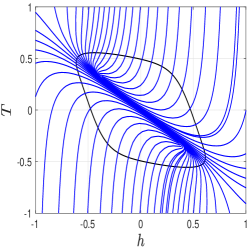
The Jin model’s nonlinearity reflects the nonlinear vertical distribution of the temperature in the tropical upper ocean. Such a nonlinear dependence on subsurface temperature in the (western) thermocline depth is obtained by adding a term proportional to (the eastern thermocline depth) into the SST equation following ideas commonly employed in ENSO modeling BH89 ; Zebiak_al87 ; Neelin_al98 which through ocean-atmosphere coupling through winds leads to the nonlinearity in the SST eastern equation of Eq. (7); see (jin1997equatorial, , Eqns. (2.1) and (3.1)) for details. This nonlinearity is crucial for capturing the oscillatory nature of ENSO. In its standard parameter regime, the model leads to a limit cycle known as the ENSO fundamental oscillation jin1997equatorial . This periodic oscillation is shown in Fig. 1 along with a few of its isochrons characterizing the nonlinear relaxation towards it; see Section II.2.
When the perturbation terms are stochastic, they are often sought for accounting for uncertainties, variability, and potential missing physics that might be difficult to capture deterministically in such simplified, conceptual models csg11 . Intuitively, the presence of stochastic terms can help capture the intermittent nature of ENSO events, by attributing the irregular occurrence of strong El Niño or La Niña episodes to the interplay between stochastic fluctuations and nonlinear ENSO features roulston2000response ; lengaigne2004triggering ; fedorov2015impact , encoded here by the ENSO limit cycle in the Jin’s recharge oscillator model.
The plausibility of a stochastic forcing as a mechanism for ENSO irregularity has been argued in many studies. Physical origins of such a forcing include large-scale synoptic atmospheric transients such as the Madden Julian Oscillation batstone2005characteristics or westerly wind bursts roulston2000response ; fedorov2002response ; lengaigne2004triggering ; fedorov2015impact . Dynamically, the idea is to explicitly separate the slow and fast modes in the atmosphere and add the latter to simple deterministic models as a stochastic forcing term. Other sources of stochasticity include processes associated with atmospheric/moist convective disturbances whose timescales can vary from hours to weeks. Typically, the additional fast-mode random forcing disrupts the slow scales and convert the original periodic or damped oscillation supported by the deterministic model into an irregular one with a diversity of El Niño events. Such dynamical behaviors have been previously documented through a combination of data-driven models built from observational data penland1995optimal ; kondrashov2005hierarchy ; CKG11 ; chen2016diversity as well as through a hierarchy of ENSO models including general circulation models lengaigne2004triggering ; fedorov2015impact , intermediate-complexity models blanke1997estimating ; chen2018observations ; eckert1997predictability ; thual2016simple ; roulston2000response ; zavala2003response , or other conceptual models chen2022multiscale ; chen2023rigorous ; chekroun2024effective .
In this study, we aim at analyzing the type of ENSO irregularity that is produced by applying a new type of stochastic parameterizations designed in (Chekroun_al22SciAdv, ) to produce enriched temporal variability out of periodic oscillations.
II.2 Shear-induced chaos caused by jump-diffusion processes
Reference Chekroun_al22SciAdv introduced a general framework for generating solutions with enhanced temporal variability by applying stochastic perturbations to systems exhibiting a fundamental oscillation (limit cycle). The limit cycle’s isochrons guckenheimer1975isochrons ; Ashwin2016 , representing level sets of the oscillation’s phase function, are pivotal in determining the system’s response to spike winfree1980geometry ; izhikevich2007dynamical or stochastic perturbations (Chekroun_al22SciAdv, ). The more their twist is pronounced, the more the system is susceptible to produce shear-induced chaos lin2008shear ; Young2016 , with a stochastic attractor characterized by stretching and folding in the state-space, indicative of (stochastic) Smale’s horseshoes. Reference (Chekroun_al22SciAdv, ) introduces a practical method to systematically enhance stochastically the isochrons’ twist, promoting thus the emergence of such chaotic behavior. This leads to solutions with increased temporal variability, complexity, and broader frequency spectra, improving model realism for various applications. Figure 1 shows a few isochrons computed for the Jin model’s limit cycle following the algorithm given in (izhikevich2007dynamical, , Chapter 10). We refer to guillamon2009computational ; detrixhe2016fast for other algorithms to compute isochrons in dimension greater than two (iso-surfaces).
Guided by the stochastic parameterization approach of Chekroun_al22SciAdv , we propose thus to apply to the Jin model (Eq. (7)), the following state-dependent stochastic disturbances:
| (8) |
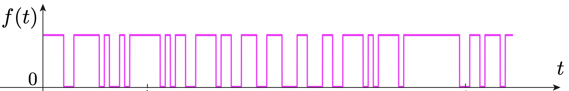
where is a jump process that corresponds to a random comb signal, where the activation events (represented by the pulses) occur at random times. More precisely, given a firing rate in , and duration , we define thus as the following real-valued jump process:
| (9) |
where is a uniformly distributed random variable taking values in and if and only if . A realization of is shown in Fig. 2. This type of jump process is also known as a dichotomous Markov noise bena2006dichotomous , or a two-state Markov jump process in certain fields stechmann2011stochastic . It is encountered in many applications horsthemke1984noise . Note that the Wiener processes and the jump process are taken to be mutually independent.
These stochastic terms are aimed at capturing nonlinear and intermittent processes that are not represented in the simplified Jin’s recharge oscillator model. These might include complex ocean-atmosphere interactions, the role of oceanic current and eddies, or atmospheric teleconnections. For instance, the term multiplied by the jump process in the -term, affecting the temperature equation in Eq. (7), can be thought as caused by nonlinear and intermittent thermocline upwelling and advective feedback processes. In the original Jin model jin1997equatorial , the term in the -equation expresses a simple proportional relation between the wind stress and SST anomalies. The multiplicative jump term in of Eq. (8) aims thus at accounting for extra nonlinear and feedback mechanisms between the wind stress and SST anomalies which are present in more elaborated, spatially-extended models of ENSO; see Zebiak_al87 ; Jin_al93_part1 ; Jin_al93_part2 ; Dijkstra05 ; cao2019mathematical and references therein.

We mention that the effects of state-dependence noise on ENSO dynamics is an ongoing research topic jin2007ensemble ; sardeshmukh2015understanding , and in that sense our noise proposal in Eq. (8) involving jump process and different state-dependences than in previous studies, is aimed at providing new insights on this topic.
We write finally Eq. (7) subject to stochastic disturbance (8) into the following compact form:
| (10) |
where , , and the components of the drift term are given by
| (11) | ||||
while the multiplicative factor of the jump process is given by
| (12) |
As detailed in Chekroun_al22SciAdv in a general context, generating shear-induced chaos from Eq. (10) using perturbations of the form requires a careful selection of the firing rate. This rate must be sufficiently low to enable nonlinear relaxation towards the limit cycle while remaining high enough to maintain the impact of random kicks. Both aspects are essential for stretch-and-fold dynamics to take place. The perturbation magnitude also plays a critical role. In agreement with theoretical predictions of Chekroun_al22SciAdv , appropriate combinations of random kicks (controlled by and ) and fast stochastic fluctuations (governed by ) drive strong interactions between the stochastic forcing and the Jin model’s nonlinear dynamics near its limit cycle. This interplay leads eventually to shear-induced chaos, as evidenced by the stretching and folding patterns shown in Figure 3A-C. The specific noise parameters for this chaotic regime are listed in Table 2 (Case B).
| 1 | 0.125 |
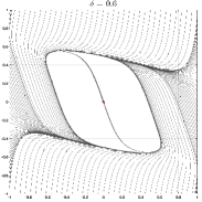
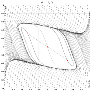
Note that in our notations, the bifurcation control parameter used by Jin in jin1997equatorial is recovered as . The parameter is thus our bifurcation parameter here. For used in most of our numerical experiments below the system exhibits a stable limit cycle that bifurcated from an unstable equilibrium. As noted by Jin in jin1997equatorial the system exhibits the emergence of two new unstable steady states as approaches ; see Fig. 4.
| Case A: | N/A | N/A | N/A | N/A | ||
| Case B: | 0.7 | 0.7 | 0.1 |
Our goal is to provide new insights on this type of stochastic chaos by computing the underlying Kolmogorov modes, linear response and Green functions from statistical physics. To do so, we generalize below these concepts to Lévy diffusion processes from which shear-induced chaos becomes a special case (Section III.3). As shown in Section V.2, the theory is particularly useful for predicting via linear response theory how changes in ocean-atmosphere coupling (i.e. in the parameter ) affect the system’s behavior.
III Fokker-Planck Equation of Lévy-driven Dynamics
III.1 Kolmogorov operator of Lévy-driven dynamics
There is a vast literature on Lévy processes which roughly speaking are processes given as the sum of a Brownian motion and a jump process tankov2003financial ; peszat2007stochastic ; Applebaum2009 ; kuhn2017levy ; oksendal2019stochastic . Unlike the case of Gaussian diffusion processes (SDEs driven by Brownian motions), the representation of Kolmogorov operators is non-unique in the case of Lévy-driven SDEs, and may take the form of operators involving fractional Laplacians or singular integrals among other representations Kwasnicki:2017aa . We adopt here the definition commonly used in probability theory (Applebaum_2019, , Theorem 3.5.14) which presents the interest of being particularly intuitive as recalled below.
We consider SDEs in of the form:
| (13) |
where and are assumed to be respectively a Brownian motion and a Lévy process in , that are mutually independent. To simplify, we assume here that the covariance matrix is a definite matrix for each .
Roughly speaking, a Lévy process on is a non-Gaussian stochastic process with independent and stationary increments that experience sudden, large jumps in any direction. The probability distribution of the these jumps is characterized by a non-negative Borel measure defined on and concentrated on that satisfies the property . This measure is called the jump measure of the Lévy process . Sometimes itself is referred to as a Lévy process with triplet . Within this convention, we reserve ourselves the terminology of a Lévy process to a process with triplet . We refer to Applebaum2009 and peszat2007stochastic for the mathematical background on Lévy processes.
Under suitable assumptions on , , and the Lévy measure , the solution to Eq. (13) is a Markov process (e.g. protter2005stochastic ) and even a Feller process kuhn2018solutions , with associated Kolmogorov operator, which extends the one shown in Eq. (6), taking the following integro-differential form for (e.g.) in (Courrège theorem courrege1965forme ; kuhn2017levy ):
| (14) | ||||
where denotes the indicator function of the (open) unit ball in ; see also (Applebaum2009, , Theorem 3.3.3). We will call the Kolmogorov-Lévy operator to make the distinction with the Kolmogorov operator in the pure diffusive case.
The first-order term in Eq. (14) is the drift term caused by the deterministic, nonlinear dynamics. The second-order differential operator represents the diffusion part of the process . It is responsible for the continuous component of the process.
The -term, involving the integral, represents the jump part of the process. It captures the discontinuous jumps that the process experience due to the sudden changes caused by the Lévy process . Its intuitive interpretation breaks down as follows. The term, , calculates the difference in the test function value before and after the potential jump, capturing the change in the test function due to the jump.
The term represents a first-order correction for small jumps. It aims to account for the fact that a small jump might not land exactly on the grid point (), but somewhere in its vicinity. This term is often referred to as the Girsanov correction. Thus, the integral term accounts for all possible jump sizes () within a unit ball, as weighted by the Lévy measure .
The Kolmogorov-Lévy operator such as given by Eq. (14) generates a strongly continuous semigroup (-semigroup) (Applebaum_2019, , Theorem 3.5.14). This semigroup has the following characterization Applebaum2009 :
| (15) |
i.e. it provides the expected value of an observable over the stochastic solution paths that connect in to solving Eq. (13) at time . The semigroup gives thus a deterministic macroscopic description of the averaged effects of the combined Lévy flights and Brownian motions driving the dynamics.
Thanks to semigroup theory, following Chekroun_al_RP2 , correlation functions and power spectra benefit of decomposition formulas such as given by Eqns. (23) and (26), in which the corresponding RP resonances and Kolmogorov modes are now the spectral elements associated with the isolated part of . This is clarified in Section IV.1 below.
The direct numerical approximation of such Kolmogorov-Lévy operator is however a non-trivial task, requiring in particular a special care to handle the singular integral involved therein gao2014mean ; gao2016fokker . We take below in Section IV.2 another route to estimate the RP resonances and Kolmogorov modes, based instead on the Ulam’s method ulam1960collection , a data-driven approach that has proven its efficiency for chaotic and pure diffusion dynamics driven by Brownian motion; see junge2009discretization ; Chek_al14_RP ; Chekroun_al_RP2 .
III.2 Fokker-Planck Equation of Lévy-driven Dynamics
The Fokker-Planck equation provides the governing equation of the transition probability density , i.e. the probability of the process has value at time given it had value at time . We denote by this transition probability that we assume to be smooth with respect to the Lebesgue volume; see picard1996existence ; priola2009densities ; priola2012pathwise and (kuhn2017levy, , Sec. 5.5) for conditions. Then, in many cases, the Fokker-Planck equation associated with Eq. (13) (in ) is given by the following non-local integro-differential equation:
| (16) | ||||
For conditions ensuring the Kolmogorov-Lévy operator to be the infinitesimal generator of a strongly continuous semigroup in spaces (), we refer to garroni2002second ; chen2010heat ; applebaum2021 . In compact form, Eq. (16) can be written as
| (17) |
where denotes the integral term in Eq. (16), which is associated with the jump processes. Formally, where denotes the adjoint of the Kolmogorov operator given by Eq. (14).
There exists a well-known equivalent representation of Eq. (16) when is the Lévy measure:
| (18) |
associated with an -stable Lévy process. Here lies in and is called the non-Gaussianity index and is a constant that depends on the dimension and involves the function of Euler Kwasnicki:2017aa . A -stable () process is simply a Brownian motion.
For any such (general) -stable Lévy process, one can recast Eq. (16) by means of the fractional Laplacian , which is associated with a fat-tailed dispersal kernel (for in ) and therefore describes long-distance dependencies. The equivalent formulation is then written as (e.g. (schertzer2001fractional, , Eqns. (57)-(58)) and (priola2012pathwise, , Eq. (6))):
| (19) | ||||
where the fractional Laplacian is defined using the following Riesz’ representation formula albeverio2000invariant :
where denotes the Fourier transform of , given by and its Fourier inverse. Recall that the limiting case corresponds to the Brownian motion which is recovered formally by setting in Eq. (19).
III.3 Kolmogorov operator of the stochastic Jin’s model
We go back now to the case of the stochastic Jin’s model given by Eq. (10) and write down the corresponding Kolmogorov-Lévy operator. The difference with what precedes lies in the state-dependent form of the jump perturbations. Still, the formalism recalled above allows us to deal with this situation with ease as explained below.
To do so, we first write down the Kolmogorov operator associated with Eq. (10) in the case (no jump). It is given by (see Eq. (6))
| (20) |
where .
Since in Eq. (10), the (scalar) jump perturbations are multiplied by the vector , the Kolmogorov operator Eq. (14) takes here the form
| (21) |
where the jump measure is the measure associated with the real-valued jump process . The latter is the Dirac delta , where is the intensity of the Poisson process associated with the jump process. Recall that this intensity is the limit of the probability of a single event occurring in a small interval divided by the length of that interval as the interval becomes infinitesimally small.
Consider a small time interval . The probability of an event occurring in this interval is given by the probability that the random variable falls within the range . Since is uniformly distributed, this probability is simply . The expected number of events in the interval is the product of the probability of an event and the length of the interval. Therefore, the expected number of events is and .This means that the expected number of activation events in any given time interval is proportional to the length of that interval and the firing rate.
As a consequence, Eq. (21) simplifies to
| (22) |
The next section (Sec. IV) introduces the notions of Ruelle-Pollicott (RP) resonances and Kolmogorov modes for general Kolmogorov operators such as given by Eq. (14). The particular case of the Kolmogorov operator given by Eq. (22) is dealt with in Section IV.3.
IV Ruelle-Pollicott Resonances and Kolmogorov Modes
IV.1 Correlations and power spectra decompositions
As detailed in Chekroun_al_RP2 for a broad class of stochastic systems driven by Brownian motion, the RP resonances correspond to the isolated eigenvalues of the system’s Kolmogorov operator while the Kolmogorov modes are its eigenfunctions. These modes and resonances hold significant importance. They enable the derivation of rigorous decomposition formulas for both temporal correlation functions and power spectral density functions across a wide range of physical stochastic systems. These decomposition formulas can be made rigorous for general stochastic systems including the hypoelliptic ones Chekroun_al_RP2 ; see also dyatlov2015stochastic .
We present below the extension of these formulas for SDEs driven by Lévy processes, of the form given by Eq. (13). For the sake of simplicity, we do not (unlike in Chekroun_al_RP2 for Brownian-SDEs) enter into the precise conditions on , , and that ensure (i) the SDE to possesses a unique ergodic invariant measure , and (ii) to generate a -semigroup on .
The study of existence of invariant probability measures albeverio2000invariant ; kulik2009exponential ; behme2015criterion ; behme2024invariant , and ergodic properties of Lévy processes in terms of the coefficients of the corresponding infinitesimal generator (the Kolmogorov-Lévy operator) is an ongoing research topic.
We refer to masuda2004multidimensional ; kulik2009exponential ; sandric2016ergodicity for useful criterions regarding the exponential ergodicity when the coefficients are locally Lipschitz continuous, and to xie2020ergodicity for more general conditions allowing for large jumps.
Once (i) and (ii) are ensured, we can apply (Chekroun_al_RP2, , Corollary 1) and thus obtain for any observables and (square-integrable w.r.t. system’s ergodic probability measure):
| (23) |
where the reminder satisfies , and the coefficients are given by (Chekroun_al_RP2, , Eq. (2.11))
| (24) |
in which (resp. ) denotes the eigenfunction (dual eigenfunction) associated with the RP resonances , denotes the -Hermitian inner product, while correspond to the (algebraic) multiplicity of these resonances. Note that in the above decomposition, we assumed that the observables have been centered, i.e. that the mean with respect to the ergodic measure has been subtracted.
For these systems, the spectrum of the Kolmogorov operator is typically contained in the left-half complex plane eckmann2003spectral ; Chekroun_al_RP2 , and its resolvent , is a well-defined operator that possesses the following integral representation
| (25) |
The RP resonances correspond then to the poles of the resolvent , and the to the orders of these poles. The location of these poles are independent of the observables but their relative importance (through the coefficients depend on them. It is noteworthy that the theory of RP resonances has been initially introduced for deterministic chaotic systems ruelle1986locating ; pollicott1986meromorphic ; keller1999stability ; baladi2000positive ; gaspard2005chaos and is an active field of research faure2011upper ; giulietti2013anosov ; dyatlov2019mathematical .
The theory for chaotic systems is however much more challenging as the underlying ergodic measure of physical interest is typically singular with respect to the Lebesgue measure, requiring in particular the use of special function spaces to study the spectral properties of these resonances butterley2007smooth ; faure2011upper ; gouezel2006banach . The improved regularity due to noise diffusion simplifies considerably key aspects of the problem Hairer_Majda allowing us in particular to rely here on semigroup theory Engel_Nagel in standard function spaces to derive correlation decomposition formulas such as Eq. (23); see Chekroun_al_RP2 . RP resonances have been shown also to be instrumental in the diagnosis of efficient stochastic parameterizations for the reduced-order modeling of nonlinear systems with complex dynamics Kondrashov_al2018_QG ; chekroun2021stochastic .
A useful consequence of Eq. (23) is the decomposition of the power spectrum, , in terms of RP resonances and Kolmogorov modes following Chekroun_al_RP2 . The latter is obtained by taking the Fourier transform of the correlation function (Wiener-Khinchin theorem), which gives e.g. in the case of poles of order (),
| (26) |
where is a complex frequency and denotes some “background” function decaying to as ; see also melbourne2007power . Eq. (26) shows that the meromorphic extension into the complex plane of the power spectrum when is real, present poles that are exactly given by the RP resonances. These poles manifest themselves in the (real) power spectrum as peaks that stand out over a continuous background at frequencies given by the imaginary part of the eigenvalues, when and if the are close enough to the imaginary axis.
Thus, the RP resonances and Kolmogorov modes characterize the various ways a system’s stochastic dynamics expresses its temporal variability through observables.
IV.2 Ulam’s estimation of RP Resonances and Kolmogorov modes
Analytical formulas for RP resonances and Kolmogorov modes are scarce (see, e.g., metafunes2002 ; gaspard1995 ; gaspard2002trace ; gardiner2009 ; pavliotisbook2014 ; Tantet_al_Hopf ). In practice, these resonances are estimated e.g. from long time series obtained by solving the governing equations (e.g., Eq. (10)); crommelin2011diffusion ; generatorfroyland ; Chekroun_al_RP2 .
Leveraging the Ulam method ulam1960collection , Markov matrices are crucial for both learning transfer operator properties and estimating the system’s propagator’s long-term behavior; e.g. schutte1999direct ; junge2009discretization ; Froyland2021 . This propagator governs the evolution of probability densities and reveals also how correlations and other system aspects change over time froyland2003detecting ; Chek_al14_RP ; generatorfroyland . This approach applies to both deterministic and stochastic systems froylandapproximating1998 ; fishman2002 ; Chekroun_al_RP2 .
Ulam’s method provides thus a way to estimate the propagator using Markov transition matrices. Eigenvalues of the Kolmogorov-Lévy operator are then obtained through logarithm formulas crommelin2011diffusion ; Chekroun_al_RP2 . This method consists of subdividing the state space , typically shadowing the dynamics’ forward attractor, into non-intersecting cells or boxes and estimating the dynamics’ probability transitions across these boxes. Mathematically, the propagator, , for a given transition time , is approximated by a Markov transition matrix , whose entries are given by Chekroun_al_RP2 :
| (27) |
for , where denotes the indicator function on the box , denotes the system’s ergodic invariant probability measure and , a given initial distribution. The transition matrix is then estimated by computing a classical maximum likelihood estimator given by crommelin2011diffusion ; schutte1999direct :
| (28) |
for . Given a sampling time at which the time series solving Eq. (10), is collected, the formula (28) counts the number of observations () visiting the box after iterations, knowing that it already landed in . The resulting operation results into a coarse-graining of the dynamics encoded by crommelin2006b ; Chekroun_al_RP2 that incorporates artificial diffusion generatorfroyland , of minor impact when and are sufficiently large. Note that for high-dimensional systems, time series constructed from reduced coordinates (observables) are often used instead of the full-state vector for obvious computational reasons. In this case, transition matrices can still be estimated in a reduced state space and their eigenvalues can still be informative about the genuine system’s transitions (in the full state space) through the notion of reduced RP resonances; see (Chek_al14_RP, , Theorem A) and Chekroun_al_RP2 ; RP_ENSO .
IV.3 Stochastic Jin model’s RP resonances and Kolmogorov modes
We follow the procedure just recalled by integrating the stochastic Jin model (10) via an Euler-Miruyama scheme with a time-step . Two cases of stochastic disturbances are considered as listed in Table 2. The underlying time series are obtained by collecting sequential data points (after transient removal) by sampling every time-steps numerical solutions to Eq. (10) made of data points. Markov transition matrices with and built up out of cells shadowing the resulting cluster of data points in the -plane, are then estimated according to the Ulam’s procedure recalled above. The dominant spectral elements are computed using standard routines. The corresponding eigenvalues are shown below after taking the logarithm.
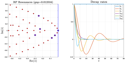
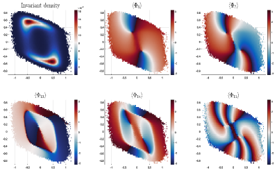
The results are shown in Figures 5-6 for Case A, and in Figures 7-8, for Case B. The phase (in ) of the Kolmogorov modes are shown for the RP resonances circled in blue. Note that in Case A () one recovers the parabolic shape formed by the dominant resonances, enveloping a triangular array of resonances as in the case of the Hopf normal form subject to a small additive white noise Tantet_al_Hopf . As explained in Tantet_al_Hopf , the triangular array of resonances is associated with the unstable steady state while the parabola is associated with the random stable limit cycle. The phase of two modes composing this triangular array are shown as and in Fig. 6. Their structures differ notably from those associated with the parabola of resonances. The latter modes whose phase is shown as , , and in Fig. 8 are characterized by level sets organized by the unperturbed system’s isochrons (see Fig. 1)—here orthogonal to these, as already pointed in Tantet_al_Hopf for the case of the Hopf normal form. Note that the isochrons are known to provide exactly the level sets of certain Koopman eigenfunctions for pure deterministic oscillations mauroy2012use .
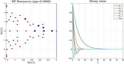
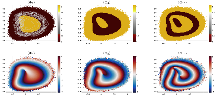
The modes and resonances associated with Case B, i.e. when the state-dependent jump-noise is activated, show different attributes. The spectral gap is noticeably increased in Case B compared to Case A, indicative of a stronger mixing in the state space and faster decay of correlations. We observe also that the parabola and triangular array formed by the resonances in Case A are now destroyed, giving rise to another discrete geometry of the spectrum. A remarkable feature though is the presence of real resonances that extend until the deep part of the spectrum as one moves leftward in the complex plane. The corresponding real modes display positive and negative areas that are better revealed when plotting their phase as shown in the top row of Figure 8, with phase equals to corresponding to negative values (yellow zones) and phase equals to corresponding to positive values (brown zones).
Mode , associated with the slowest decaying eigenvalue in Figure 7, reveals two distinct regions. The brown region corresponds to the most frequently visited area of the state space by the dynamics of Eq. (10). Moving leftward in the complex plane, the real modes delineate concentric regions of positive and negative values, corresponding to varying sojourn time statistics. While a detailed analysis of these statistics is beyond this paper’s scope, the capability of real Kolmogorov modes to identify regions with potentially rare events (characterized by short sojourn times) warrants attention.
The phase of the (purely) complex Kolmogorov modes reveal striking features. Their phase is noticeably exhibiting spiraling patterns reflecting the underlying stretch-and-fold dynamics displayed by the stochastic attractor (Figure 3A-C), with the order of these spiraling patterns (its “winding number”) that increases as one moves leftward in the complex plane; see bottom row of Figure 8. Overall, they also account for the rotation imposed by the specific form of the state-dependent component in Eq. (8), i.e. the -term (Eq. (12)).
Recall that provides the deterministic macroscopic description of the averaged effects of the combined Lévy flights and Brownian motions (see Eq. (15)). By using the decomposition theorem of -semigroups in our context (Engel_Nagel, , Theorem V.3.1) and since the RP resonances are here simple, we obtain, by summing up over the dominant RP resonances, that
| (29) |
with decaying exponentially to at a controlled rate as ; see (Chekroun_al_RP2, , Theorem 1). Here denotes the weighted "half"-inner product with respect to the system’s (ergodic) invariant measure , by the -Kolmogorov mode of the Fokker-Planck operator given by the RHS of Eq. (16), and associated with the RP resonance .
Thus for any smooth observable , since is also equals to with solving the Fokker-Planck equation Eq. (16), we arrive at the formula
| (30) |
with decaying exponentially to at a controlled rate as . In particular, this formula provides the rate of convergence of any moment statistics (for instance by taking ) and allows for identifying the Kolmogorov mode(s) controlling this rate of decay. This semi-analytical/empirical observation hints towards an actual exponential ergodicity for the actual stochastic Jin’s model Eq. (10) whose rigorous proof goes beyond the scope of this paper; see masuda2004multidimensional ; kulik2009exponential ; sandric2016ergodicity for theoretical frameworks.
Recall also that the Kolmogorov modes provide the characteristic patterns in the state space, that encode the system’s variability due to the decomposition formula of power spectra Eq. (26). Adopting the language of climate change, they provide the modes of the system’s natural variability, prior a perturbation is applied and are thus of utmost importance.
Note that although the Ulam’s approach enables us to reveal with accuracy key features of the Kolmogorov modes here, it performs poorly to resolve the modes’ details at the periphery of the available data points. Other data-driven approaches using e.g. the extended dynamic mode decomposition could be used to address this issue williams2015data ; klus2018data , although such alternative method could encounter other difficulties boiling down to the appropriate choice of basis functions, tied to the intricate spiraling structures exhibited by the (purely complex) Kolmogorov modes lying in the deeper part of the spectrum.
The next section highlights another key property of Kolmogorov modes: their ability to encode the system’s response to general perturbations of the drift term () through Green functions.
V Linear Response of Lévy-driven Dynamics
V.1 Green’s Function of Lévy-driven Dynamics
Leveraging the formalism of Section III for Kolmogorov operators and Fokker-Planck equations for Lévy-driven stochastic systems of the form of Eq. (13), we can directly extend the FDT relationships discussed in Section I.1 to these more general systems. To do so, we follow the approach outlined in Section I.1 and consider perturbations to the drift term of the following form:
| (31) | ||||
where is time-dependent scalar modulation function and is the drift perturbation.
Using Eq. (19), we obtain that the evolution of probability density functions associated with Eq. (31) is given by the Fokker-Planck equation
| (32) | ||||
where denotes the integral term in Eq. (16).
Let us expand the statistical state, , solving the time-dependent Fokker-Planck equation (32):
| (33) |
where , denotes the reference, statistical equilibrium given as the system’s ergodic probability density for that we assume here to exist (see masuda2004multidimensional ; kulik2009exponential ; sandric2016ergodicity for conditions).
To obtain , we plug given by Eq. (33) into Eq. (32) and retain the first-order terms in . By using the semigroup providing the solution operator to the Fokker-Planck Eq. (32), with denoting the dual of the Kolmogorov-Lévy operator (given explicitly as the right-hand side of Eq. (16)), we obtain then
| (34) |
where
| (35) |
The expected value of at time , for the statistical state is then given by
| (36) | ||||
After integrating by part we arrive at
| (37) |
where is the (causal) Green’s function given by:
| (38) |
in which is the Heaviside function. Structurally, one recovers the same response operator as for the case of stochastic systems driven by Gaussian noise (Sec. I.1) in which the Kolmogorov operator for pure diffusion (Eq. (6)) has been replaced by the Kolmogorov-Lévy operator.
Here also, the (genuine) ensemble anomaly at time , , with respect to the reference state , is approximated—at the leading order in —by the anomalies obtained by the linear response formula:
| (39) |
As discussed in Section I.1, the Green’s function can also be interpreted as time-lagged correlations between the observables and , involving only the statistics of the unperturbed system. In that sense, it provides a general version of the FDT Kubo1966 ; majda2005information valid for jump-diffusion models.
Using then the decomposition of (temporal) correlations in terms of Kolmogorov modes (Chekroun_al_RP2, , Corollary 1) (see Eq. (23)) the Green function can be approximated as
| (40) |
with when , and where the coefficients are given by:
| (41) |
by application of Eq. (24) with and . Thus, the ’s weight, according to Eq. (41), the contribution of the Kolmogorov modes to the response for a given observable and forcing pattern defining the operator given by Eq. (35).
V.2 Applications to the jump-diffusion Jin model
In this section, we apply the above linear response framework to the jump-diffusion Jin model given by Eqns. (10)-(12). We are interested in predicting the response of this jump-diffusion model to small perturbations of the drift term in this model.
We consider the physically relevant situation where the ocean-atmosphere coupling parameter is allowed to be varied as . This parameter variation impacts the two components of the drift in Eq. (11) as follows:
| (42a) | ||||
| (42b) | ||||
At first sight, due to the presence of higher-order terms in , this choice of parameter variation does not seem to fit within the linear response framework of Section V.1, in which is perturbed into . However, LRT aims at assessing the impacts on statistics at the leading order in and therefore accounting for contributions of the quadratic and cubic terms in from Eq. (42b), are irrelevant at this level of approximation. We can thus theoretically frame our experiments as corresponding, up to linear terms in , to the following perturbation:
We first adopt an empirical, direct approach following gritsun2017 to estimate the system’s response to parameter variations. In that respect, we sample points from a long unperturbed system run (), distributed according to the invariant measure . For each ensemble member, we apply a perturbation and estimate the response , where denotes the ensemble average over the perturbed system relative to the forcing and amplitude .
Then, following gritsun2017 , we extract the linear component of the response using a centered difference approximation:
| (43) |
For small but finite , this approximation effectively eliminates the quadratic response term and provides a robust estimate of the linear component.
For a given forcing , we implement two sets of response experiments with amplitudes . Extracting a linear response signal from numerical experiments involves careful considerations and trade-offs. The perturbation amplitude should be large enough to maximize the signal-to-noise ratio but small enough to avoid nonlinear effects. A large ensemble size is also crucial to reduce fluctuations arising from the system’s chaotic dynamics and its inherent stochasticity tied to jump process. Generally, smaller perturbation amplitudes require larger ensemble sizes to confidently extract a linear response signal.
We apply this empirical approach to the case of a step perturbation Lucarini2017 , corresponding to a sudden change in the ocean-atmosphere coupling parameter. We evaluate the system’s response for different perturbation magnitudes, , where .
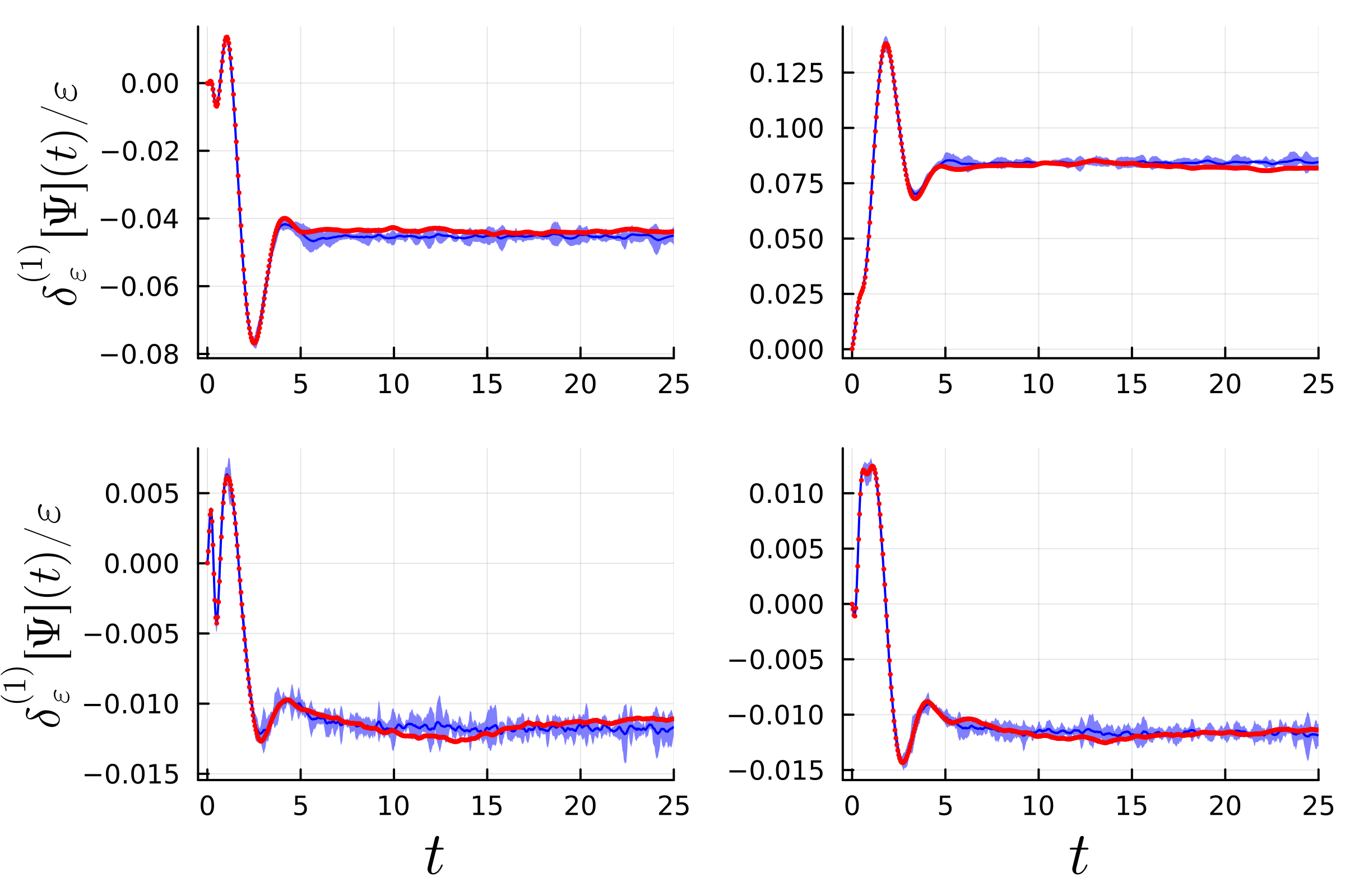
Figure 9 shows that the linear response can be reliably extracted for perturbations up to of the original value. This indicates a robust range of validity for the linear response approximation. The blue curve represents the mean rescaled response across different values, while the shaded area denotes the fluctuations estimated, at each point in time, as . These results confirm that the system (Eq. (10)), despite its discontinuous jump process component (), exhibits smooth statistical dependence on the perturbation parameter and, consequently, on the ocean-atmosphere coupling parameter .
To further validate LRT, we compare these empirical results with the Green function formalism of Section V.1. In that respect, we compute the Green’s function of the system, from carefully designed response experiments and use it to predict the response to a step perturbation. According to LRT, the response to any time-dependent forcing can be reconstructed from the Green’s function as given by Eq. (39).
To estimate the Green’s function, we apply a short-duration perturbation over a single time step . By considering perturbations of different amplitudes, we reliably estimate (not shown). The response to a step perturbation is then calculated using:
| (44) |
due to Eq. (39).
Figure 9 demonstrates excellent agreement between the brute-force response (blue curve) and the estimate obtained from the Green’s function (red dots), further supporting the validity of linear response theory.
The state-dependent jump process and its interaction with the system’s nonlinearity can introduce persistent fluctuations, making it difficult to isolate the smooth response properties. To reliably estimate the linear response, we employed a large ensemble size ( for step perturbations and for the Green’s function). Despite the effects caused by the jump process, the underlying linear response signal remains detectable.
We focused on the response of highly fluctuating variables like powers of and . For spatially-extended, high-dimensional systems, estimating the Green’s function for spatially averaged observables may require fewer ensemble members, as spatial averaging can mitigate jump-induced fluctuations. This is particularly relevant in cases like convective parametrization, where local conditions determine transitions between convective and non-convective states, often lacking significant spatial coherence. Recent studies on using LRT for climate response predictions have shown that increased model complexity and spatial resolution can reduce the required ensemble size Lucarini2017 ; Lembo2020 .
VI Discussion
Understanding the class of dynamical systems for which linear response theory can be applied and deriving applicable linear response formulas is a significant area of research across mathematics, physics, and various fields of science that deal with complex systems. The validity of response theory has broad applications, including predicting future changes in response to external forcings, assessing sensitivity to parameter changes for model tuning, and addressing optimization problems like anticipating adversarial attacks, i.e. understanding which perturbations can cause the largest response in a system.
As recalled in the Introduction, for a large class of diffusion processes, response operators can be expressed as time-lagged correlations between system’s observables, generalizing the classical FDT. By employing the Kolmogorov operator formalism, we have clarified the link between forced and free fluctuations and decomposed response operators into terms associated with specific modes of variability (with their own decay of correlation) of the unperturbed system. This approach has the added benefit of clarifying the conditions under which critical transitions emerge through the dominant spectral gap Chek_al14_RP and defining the critical mode associated with the occurrence of the divergent behavior Lucarini2020 ; Chekroun_al_RP2 ; LucariniChekroun2023 ; Zagli2024 .
Using the Kolmogorov operator formalism (Section III.1), we have successfully extended response theory to mixed jump-diffusion models (Section V.1), which involve both Gaussian and discontinuous stochastic forcing (jumps). While the inclusion of jumps introduces nonlocal terms into the Fokker-Planck equation (Section III.2), the linearity of the equation remains intact, allowing us to apply perturbation techniques. Moreover, the decomposition of response operators using Kolmogorov modes provides a clear framework for analysis and decomposition of the response operator in terms of modes of variability, still applies (Sections IV and V.1).
We have applied our theoretical framework to analyze the response to parameter variations, of the Jin recharge model jin1997equatorial subject to state-dependent jumps and additive white noise (Section V.2). These jump-diffusion perturbations are aimed at capturing intermittent processes accounting for extra nonlinear and feedback mechanisms between the wind stress and SST anomalies which are present in more elaborated, spatially-extended models of ENSO Zebiak_al87 ; Jin_al93_part1 ; Jin_al93_part2 ; Dijkstra05 ; cao2019mathematical . They proceed from the general framework of Chekroun_al22SciAdv , and have been shown to produce generically shear-induced chaos Young2016 through the subtle interaction of jump-diffusion processes and nonlinear dynamics. Within this framework, we successfully constructed response operators and verified their accuracy.
We also computed the RP resonances and Kolmogorov modes for the shear-induced chaotic dynamics displayed by our jump-diffusion perturbed version of the Jin’s recharge model (Section IV.3). There, we have shown that such mixed stochastic perturbations responsible for the emergence of chaos, induce a larger spectral gap than in the case where the nonlinear dynamics is only subject to white noise disturbances (cf Figures 5 and 7). This increase in the spectral gap is synonymous of an enhancing of the phase-space mixing characterized by faster decay of correlations. Remarkably, in the jump-diffusion case, the Kolmogorov modes obtained from (Ulam) approximations of the Markov semigroup (Eq. (15)) display stretching and folding features (Fig. 8) characteristics of the underlying pullback attractors (Fig. 4). Roughly speaking, the expectation operator involved in Eq. (15) does not erase these important dynamical characteristics of the dynamics. Rather, these structures are still somehow encoded within the Kolmogorov modes, emphasizing the dynamical relevance of these modes.
Due to the generic character of jump-diffusion perturbations borrowed from Chekroun_al22SciAdv , and the generality of our response operators (Section V.1), it is expected that such operators are still accurate for a broad class of nonlinear systems subject to such stochastic disturbances. Following Chekroun_al22SciAdv , those include nonlinear systems supporting a high-dimensional limit cycle, to which the jump-diffusion perturbations of Chekroun_al22SciAdv are guaranteed to produce shear-induced chaos as long as a center manifold can be computed; see also lu2013strange .
High-dimensional limit cycles are found in various partial differential equations (PDEs) and time-delay models encountered in the study of climate dynamics. They play an important role in ENSO dynamics TSCJ94 ; tziperman1995irregularity ; JinEtal96 ; Galanti_al00 ; cao2019mathematical , the description of cloud-rain oscillations koren2011aerosol ; koren2017exploring , or other basic geophysical flows simonnet2003low ; Dijkstra05 ; GCS08 . We refer to dijkstra2015 ; chekroun2020efficient ; chekroun2022transitions ; chekroun2024effective for center manifold calculations in such a high-dimensional setting.
Our response operators could also be highly valuable for evaluating various modeling components (nonlinear and stochastic) to further enhance the impressive long-range ENSO forecast skills of the extended nonlinear recharge oscillators, recently introduced in zhao2024explainable .
While originally primarily studied in finance, interest in mixed jump-diffusion processes has expanded to various fields of science and technology. Singular perturbations also arise in models with complex decision-making structures, such as those found in climate models. For instance, the parametrization of subscale convection in the ocean and atmosphere often involves "if-then" statements to assess the stability of geophysical flows. Our results suggest that, despite these strong nonlinearities in the model formulations, linear response theory can still be applied. This strengthens the argument for using this approach to perform climate change projections with models of varying complexity and to assess the proximity to tipping points Ghil2020 ; LucariniChekroun2023 .
Finally, our results build up on the recent findings presented in LucariniChekroun_PRL2024 and provide foundational support for the use of optimal fingerprinting methods for climate change detection and attribution, thus strengthening one of the key aspect of the science behind climate change.
Acknowledgements.
This work has been supported by the Office of Naval Research (ONR) Multidisciplinary University Research Initiative (MURI) grant N00014-20-1-2023, and by the National Science Foundation grant DMS-2407484. This work has been also supported by the European Research Council (ERC) under the European Union’s Horizon 2020 research and innovation program (grant agreement No. 810370). V.L. acknowledges the partial support provided by the Horizon Europe Project ClimTIP (Grant No. 100018693) and by the EPSRC project LINK (Grant No. EP/Y026675/1). N.Z. has been supported by the Wallenberg Initiative on Networks and Quantum Information (WINQ).References
- (1) R. Kubo, “The fluctuation-dissipation theorem,” Reports on Progress in Physics, vol. 29, no. 1, pp. 255–284, 1966.
- (2) U. M. B. Marconi, A. Puglisi, L. Rondoni, and A. Vulpiani, “Fluctuation–dissipation: response theory in statistical physics,” Physics reports, vol. 461, no. 4-6, pp. 111–195, 2008.
- (3) R. Kubo, M. Toda, and N. Hashitsume, Statistical Physics II: Nonequilibrium Statistical Mechanics, vol. 31. Springer Science & Business Media, 2012.
- (4) D. Ruelle, “General linear response formula in statistical mechanics, and the fluctuation-dissipation theorem far from equilibrium,” Physics Letters, Section A: General, Atomic and Solid State Physics, vol. 245, no. 3-4, pp. 220–224, 1998.
- (5) O. Butterley and C. Liverani, “Smooth Anosov flows: correlation spectra and stability,” Journal of Modern Dynamics, vol. 1, no. 2, pp. 301–322, 2007.
- (6) D. Ruelle, “A review of linear response theory for general differentiable dynamical systems,” Nonlinearity, vol. 22, no. 4, pp. 855–870, 2009.
- (7) Q. Wang, “Forward and adjoint sensitivity computation of chaotic dynamical systems,” Journal of Computational Physics, vol. 235, pp. 1–13, 2013.
- (8) A. Ni and Q. Wang, “Sensitivity analysis on chaotic dynamical systems by Non-Intrusive Least Squares Shadowing (NILSS),” Journal of Computational Physics, vol. 347, pp. 56–77, 2017.
- (9) N. Chandramoorthy and M. Jézéquel, “Rigorous justification for the space-split sensitivity algorithm to compute linear response in Anosov systems,” Nonlinearity, vol. 35, p. 4357, jul 2022.
- (10) A. Ni, “Fast adjoint algorithm for linear responses of hyperbolic chaos,” SIAM Journal on Applied Dynamical Systems, vol. 22, no. 4, pp. 2792–2824, 2023.
- (11) V. Lucarini and S. Sarno, “A statistical mechanical approach for the computation of the climatic response to general forcings,” Nonlin. Processes Geophys, vol. 18, pp. 7–28, 2011.
- (12) A. Gritsun and V. Lucarini, “Fluctuations, response, and resonances in a simple atmospheric model,” Physica D: Nonlinear Phenomena, vol. 349, pp. 62–76, 2017.
- (13) T. Palmer, G. Shutts, R. Hagedorn, F. Doblas-Reyes, T. Jung, and M. Leutbecher, “Representing model uncertainty in weather and climate prediction,” Annu. Rev. Earth Planet. Sci., vol. 33, no. 1, pp. 163–193, 2005.
- (14) J. Berner, U. Achatz, L. Batté, L. Bengtsson, A. Cámara, H. Christensen, M. Colangeli, D. Coleman, D. Crommelin, S. Dolaptchiev, C. Franzke, P. Friederichs, P. Imkeller, H. Järvinen, S. Juricke, V. Kitsios, F. Lott, V. Lucarini, S. Mahajan, T. Palmer, C. Penland, M. Sakradzija, J.-S. von Storch, A. Weisheimer, M. Weniger, P. Williams, and J.-I. Yano, “Stochastic parameterization: Toward a new view of weather and climate models,” Bull. Amer. Met. Soc., vol. 98, no. 3, pp. 565–588, 2017.
- (15) V. Lucarini and M. D. Chekroun, “Theoretical tools for understanding the climate crisis from Hasselmann’s programme and beyond,” Nature Reviews Physics, 2023.
- (16) A. J. Majda, I. Timofeyev, and E. Vanden-Eijnden, “A mathematical framework for stochastic climate models,” Comm. Pure Appl. Math, vol. 54, no. 8, pp. 891–974, 2001.
- (17) V. Baladi, “Linear response, or else,” Proceedings of the International Congress of Mathematicians-Seoul, vol. 3, pp. 525–545, 2014.
- (18) V. Baladi, T. Kuna, and V. Lucarini, “Linear and fractional response for the SRB measure of smooth hyperbolic attractors and discontinuous observables,” Nonlinearity, vol. 30, no. 3, pp. 1204–1220, 2017.
- (19) M. Hairer and A. J. Majda, “A simple framework to justify linear response theory,” Nonlinearity, vol. 23, no. 4, pp. 909–922, 2010.
- (20) M. Santos Gutiérrez and V. Lucarini, “On some aspects of the response to stochastic and deterministic forcings,” Journal of Physics A: Mathematical and Theoretical, vol. 55, p. 425002, oct 2022.
- (21) D. Applebaum, Lévy Processes and Stochastic Calculus. Cambridge Studies in Advanced Mathematics, Cambridge University Press, 2 ed., 2009.
- (22) R. Cont and P. Tankov, Financial Modelling with Jump Processes. Chapman and Hall/CRC, 2003.
- (23) S. Lovejoy and D. Schertzer, The Weather and Climate: Emergent Laws and Multifractal Cascades. Cambridge: Cambridge University Press, 2013.
- (24) Y. Zheng, L. Serdukova, J. Duan, and J. Kurths, “Transitions in a genetic transcriptional regulatory system under Lévy motion,” Scientific Reports, vol. 6, no. 1, p. 29274, 2016.
- (25) L. Serdukova, Y. Zheng, J. Duan, and J. Kurths, “Metastability for discontinuous dynamical systems under Lévy noise: Case study on Amazonian Vegetation,” Scientific reports, vol. 7, no. 1, p. 9336, 2017.
- (26) Y. Zheng, F. Yang, J. Duan, X. Sun, L. Fu, and J. Kurths, “The maximum likelihood climate change for global warming under the influence of greenhouse effect and Lévy noise,” Chaos, vol. 30, no. 1, 2020.
- (27) V. Lucarini, L. Serdukova, and G. Margazoglou, “Lévy noise versus Gaussian-noise-induced transitions in the Ghil–Sellers energy balance model,” Nonlinear Processes in Geophysics, vol. 29, no. 2, pp. 183–205, 2022.
- (28) P. Ditlevsen, “Observation of -stable noise induced millennial climate changes from an ice-core record,” Geophysical Research Letters, vol. 26, no. 10, pp. 1441–1444, 1999.
- (29) M. Rypdal and K. Rypdal, “Late Quaternary temperature variability described as abrupt transitions on a 1/f noise background,” Earth System Dynamics, vol. 7, no. 1, pp. 281–293, 2016.
- (30) T. Solomon, E. R. Weeks, and H. L. Swinney, “Observation of anomalous diffusion and Lévy flights in a two-dimensional rotating flow,” Physical Review Letters, vol. 71, no. 24, p. 3975, 1993.
- (31) B. Khouider, A. Majda, and M. Katsoulakis, “Coarse-grained stochastic models for tropical convection and climate,” Proc. Natl. Acad. Sci. USA, vol. 100, no. 21, pp. 11941–11946, 2003.
- (32) S. N. Stechmann and J. D. Neelin, “A stochastic model for the transition to strong convection,” J. Atmos. Sci., vol. 68, no. 12, pp. 2955–2970, 2011.
- (33) C. Penland and P. Sardeshmukh, “Alternative interpretations of power-law distributions found in nature,” Chaos, vol. 22, no. 2, p. 023119, 2012.
- (34) S. Thual, A. J. Majda, N. Chen, and S. N. Stechmann, “Simple stochastic model for El Niño with westerly wind bursts,” Proceedings of the National Academy of Sciences, vol. 113, no. 37, pp. 10245–10250, 2016.
- (35) N. Chen and A. J. Majda, “Simple stochastic dynamical models capturing the statistical diversity of El Niño Southern Oscillation,” Proceedings of the National Academy of Sciences, vol. 114, no. 7, pp. 1468–1473, 2017.
- (36) N. Chen, C. Mou, L. M. Smith, and Y. Zhang, “A stochastic precipitating quasi-geostrophic model,” arXiv preprint arXiv:2407.20886, 2024.
- (37) I. Horenko, “Nonstationarity in multifactor models of discrete jump processes, memory, and application to cloud modeling,” Journal of the Atmospheric Sciences, vol. 68, no. 7, pp. 1493–1506, 2011.
- (38) M. D. Chekroun, I. Koren, H. Liu, and H. Liu, “Generic generation of noise-driven chaos in stochastic time delay systems: Bridging the gap with high-end simulations,” Science Advances, vol. 8, no. 46, p. eabq7137, 2022. doi.org/10.1126/sciadv.abq7137.
- (39) J. Wu, Y. Xu, and J. Ma, “Lévy noise improves the electrical activity in a neuron under electromagnetic radiation,” PloS one, vol. 12, pp. e0174330–e0174330, 03 2017.
- (40) R. Singla and H. Parthasarathy, “Quantum robots perturbed by Lévy processes: Stochastic analysis and simulations,” Communications in Nonlinear Science and Numerical Simulation, vol. 83, p. 105142, 2020.
- (41) A. Debussche, M. Högele, and P. Imkeller, The Dynamics of Nonlinear Reaction-diffusion Equations with Small Lévy Noise, vol. 2085. Springer, 2013.
- (42) M. D. Chekroun, A. Tantet, H. Dijkstra, and J. D. Neelin, “Ruelle-Pollicott Resonances of Stochastic Systems in Reduced State Space. Part I: Theory,” J. Stat. Phys., vol. 179, pp. 1366–1402, 2020. doi: 10.1007/s10955-020-02535-x.
- (43) K. Hasselmann, “Stochastic climate models Part I. Theory,” Tellus, vol. 28, no. 6, pp. 473–485, 1976.
- (44) A. Majda, R. V. Abramov, and M. J. Grote, Information Theory and Stochastics for Multiscale Nonlinear Systems, vol. 25. American Mathematical Soc., 2005.
- (45) V. Lucarini, F. Ragone, and F. Lunkeit, “Predicting Climate Change Using Response Theory: Global Averages and Spatial Patterns,” Journal of Statistical Physics, vol. 166, pp. 1036–1064, feb 2017.
- (46) V. Lucarini, “Revising and Extending the Linear Response Theory for Statistical Mechanical Systems: Evaluating Observables as Predictors and Predictands,” Journal of Statistical Physics, vol. 173, pp. 1698–1721, dec 2018.
- (47) D. Ruelle, “Nonequilibrium statistical mechanics near equilibrium: computing higher-order terms,” Nonlinearity, vol. 11, pp. 5–18, jan 1998.
- (48) V. Lucarini, “Response theory for equilibrium and non-equilibrium statistical mechanics: Causality and generalized kramers-kronig relations,” Journal of Statistical Physics, vol. 131, no. 3, pp. 543–558, 2008.
- (49) V. Lucarini and M. Colangeli, “Beyond the linear fluctuation-dissipation theorem: the role of causality,” Journal of Statistical Mechanics: Theory and Experiment, vol. 2012, p. 05013, 2012.
- (50) V. Lucarini and M. D. Chekroun, “Detecting and attributing change in climate and complex systems: Foundations, Green’s functions, and nonlinear fingerprints,” Physical Review Letters. In press., 2024.
- (51) G. A. Pavliotis, Stochastic Processes and Applications, vol. 60. Springer, New York, 2014.
- (52) M. Baiesi and C. Maes, “An update on the nonequilibrium linear response,” New Journal of Physics, vol. 15, p. 013004, jan 2013.
- (53) C. E. Leith, “Climate Response and Fluctuation Dissipation,” Journal of the Atmospheric Sciences, vol. 32, pp. 2022–2026, 1975.
- (54) A. Gritsun and V. Dymnikov, “Barotropic atmosphere response to small external actions: Theory and numerical experiments,” zv. Russ. Acad. Sci. Atmos. Ocean Phys., vol. 35, pp. 511–525, 1999.
- (55) R. V. Abramov and A. J. Majda, “Blended response algorithms for linear fluctuation-dissipation for complex nonlinear dynamical systems,” Nonlinearity, vol. 20, no. 12, p. 2793, 2007.
- (56) A. Gritsun and G. Branstator, “Climate response using a three-dimensional operator based on the fluctuation–dissipation theorem,” Journal of the Atmospheric Sciences, vol. 64, no. 7, pp. 2558–2575, 2007.
- (57) M. Budišić, R. Mohr, and I. Mezić, “Applied Koopmanism,” Chaos, vol. 22, no. 4, p. 047510, 2012.
- (58) M. O. Williams, I. G. Kevrekidis, and C. W. Rowley, “A data-driven approximation of the Koopman operator: Extending dynamic mode decomposition,” Journal of Nonlinear Science, vol. 25, no. 6, pp. 1307–1346, 2015.
- (59) F.-F. Jin, “An equatorial ocean recharge paradigm for ENSO. Part II: A stripped-down coupled model,” J. Atmos. Sci., vol. 54, no. 7, pp. 830–847, 1997.
- (60) M. J. McPhaden, A. Santoso, and W. Cai, Introduction to El Niño Southern Oscillation in a Changing Climate, ch. 1, pp. 1–19. American Geophysical Union (AGU), 2020.
- (61) L.-S. Young, “Generalizations of SRB measures to nonautonomous, random, and infinite dimensional systems,” J. Stat. Phys., vol. 166, pp. 494–515, 2016.
- (62) P. Imkeller and J.-S. Von Storch, Stochastic Climate Models, vol. 49. Springer Science & Business Media, 2001.
- (63) K. Hasselmann, “Multi-pattern fingerprint method for detection and attribution of climate change,” Climate Dynamics, vol. 13, no. 9, pp. 601–611, 1997.
- (64) M. Allen and S. Tett, “Estimating signal amplitudes in optimal fingerprinting, part i: theory,” Climate Dynamics, vol. 21, no. 5, pp. 477–491, 2003.
- (65) A. Hannart, A. Ribes, and P. Naveau, “Optimal fingerprinting under multiple sources of uncertainty,” Geophysical Research Letters, vol. 41, no. 4, pp. 1261–1268, 2014.
- (66) M. Pollicott, “Meromorphic extensions of generalised zeta functions,” Inventiones Mathematicae, vol. 85, no. 1, pp. 147–164, 1986.
- (67) D. Ruelle, “Locating resonances for axiom a dynamical systems,” Journal of Statistical Physics, vol. 44, no. 3-4, pp. 281–292, 1986.
- (68) S. M. Ulam, “A Collection of Mathematical Problems,” vol. 8, Interscience Publishers, 1960.
- (69) J. D. Neelin, D. S. Battisti, A. C. Hirst, F.-F. Jin, Y. Wakata, T. Yamagata, and S. E. Zebiak, “ENSO theory,” J. Geophys. Res. Oceans, vol. 103, pp. 14261–14290, 1998.
- (70) A. Timmermann, S.-I. An, J.-S. Kug, F.-F. Jin, W. Cai, A. Capotondi, K. M. Cobb, M. Lengaigne, M. J. McPhaden, M. F. Stuecker, et al., “El Niño–southern oscillation complexity,” Nature, vol. 559, no. 7715, pp. 535–545, 2018.
- (71) K. E. Trenberth, ENSO in the Global Climate System, ch. 2, pp. 21–37. American Geophysical Union (AGU), 2020.
- (72) H. Liu, I. Koren, O. Altaratz, and M. D. Chekroun, “Opposing trends of cloud coverage over land and ocean under global warming,” Atmospheric Chemistry and Physics, vol. 23, no. 11, pp. 6559–6569, 2023.
- (73) W. Cai, A. Santoso, M. Collins, B. Dewitte, C. Karamperidou, J.-S. Kug, M. Lengaigne, M. J. McPhaden, M. F. Stuecker, A. S. Taschetto, A. Timmermann, L. Wu, S.-W. Yeh, G. Wang, B. Ng, F. Jia, Y. Yang, J. Ying, X.-T. Zheng, T. Bayr, J. R. Brown, A. Capotondi, K. M. Cobb, B. Gan, T. Geng, Y.-G. Ham, F.-F. Jin, H.-S. Jo, X. Li, X. Lin, S. McGregor, J.-H. Park, K. Stein, K. Yang, L. Zhang, and W. Zhong, “Changing El Niño-Southern Oscillation in a warming climate,” Nature Reviews Earth & Environment, vol. 2, no. 9, pp. 628–644, 2021.
- (74) F.-F. Jin, H.-C. Chen, S. Zhao, M. Hayashi, C. Karamperidou, M. F. Stuecker, R. Xie, and L. Geng, Simple ENSO Models, ch. 6, pp. 119–151. American Geophysical Union (AGU), 2020.
- (75) S. Zhao, F.-F. Jin, M. F. Stuecker, P. R. Thompson, J.-S. Kug, M. J. McPhaden, M. A. Cane, A. T. Wittenberg, and W. Cai, “Explainable El Niño predictability from climate mode interactions,” Nature, vol. 630, no. 8018, pp. 891–898, 2024.
- (76) D. S. Battisti and A. C. Hirst, “Interannual variability in a tropical atmosphere-ocean model: Influence of the basic state, ocean geometry and nonlinearity,” J. Atmos. Sci., vol. 46, pp. 1687–1712, 1989.
- (77) S. E. Zebiak and M. A. Cane, “A model El Niño-Southern Oscillation,” Monthly Weather Review, vol. 115, pp. 2262–2278, 1987.
- (78) M. D. Chekroun, E. Simonnet, and M. Ghil, “Stochastic climate dynamics: Random attractors and time-dependent invariant measures,” Physica D, vol. 240, no. 21, pp. 1685–1700, 2011.
- (79) M. Roulston and J. Neelin, “The response of an ENSO model to climate noise, weather noise and intraseasonal forcing,” Geophysical Research Letters, vol. 27, no. 22, pp. 3723–3726, 2000.
- (80) M. Lengaigne, E. Guilyardi, J.-P. Boulanger, C. Menkes, P. Delecluse, P. Inness, J. Cole, and J. Slingo, “Triggering of El Niño by westerly wind events in a coupled general circulation model,” Climate Dynamics, vol. 23, pp. 601–620, 2004.
- (81) A. V. Fedorov, S. Hu, M. Lengaigne, and E. Guilyardi, “The impact of westerly wind bursts and ocean initial state on the development, and diversity of El Niño events,” Climate Dynamics, vol. 44, pp. 1381–1401, 2015.
- (82) C. Batstone and H. Hendon, “Characteristics of stochastic variability associated with ENSO and the role of the MJO,” Journal of Climate, vol. 18, no. 11, pp. 1773–1789, 2005.
- (83) A. Fedorov, “The response of the coupled tropical ocean–atmosphere to westerly wind bursts,” Quarterly Journal of the Royal Meteorological Society, vol. 128, no. 579, pp. 1–23, 2002.
- (84) C. Penland and P. D. Sardeshmukh, “The optimal growth of tropical sea surface temperature anomalies,” Journal of climate, vol. 8, no. 8, pp. 1999–2024, 1995.
- (85) D. Kondrashov, S. Kravtsov, A. W. Robertson, and M. Ghil, “A hierarchy of data-based ENSO models,” Journal of Climate, vol. 18, pp. 4425–4444, 2005.
- (86) M. D. Chekroun, D. Kondrashov, and M. Ghil, “Predicting stochastic systems by noise sampling, and application to the El Niño-Southern Oscillation,” Proceedings of the National Academy of Sciences, vol. 108, no. 29, pp. 11766–11771, 2011.
- (87) C. Chen, M. A. Cane, N. Henderson, D. E. Lee, D. Chapman, D. Kondrashov, and M. D. Chekroun, “Diversity, nonlinearity, seasonality, and memory effect in ENSO simulation and prediction using empirical model reduction,” Journal of Climate, vol. 29, no. 5, pp. 1809–1830, 2016.
- (88) B. Blanke, J. Neelin, and D. Gutzler, “Estimating the effect of stochastic wind stress forcing on ENSO irregularity,” Journal of Climate, vol. 10, no. 7, pp. 1473–1486, 1997.
- (89) N. Chen, A. J. Majda, and S. Thual, “Observations and mechanisms of a simple stochastic dynamical model capturing El Niño diversity,” Journal of Climate, vol. 31, pp. 449–471, 2018.
- (90) C. Eckert and M. Latif, “Predictability of a stochastically forced hybrid coupled model of El Niño,” Journal of Climate, vol. 10, no. 7, pp. 1488–1504, 1997.
- (91) J. Zavala-Garay, A. Moore, C. Perez, and R. Kleeman, “The response of a coupled model of ENSO to observed estimates of stochastic forcing,” Journal of Climate, vol. 16, no. 17, pp. 2827–2842, 2003.
- (92) N. Chen, X. Fang, and J.-Y. Yu, “A multiscale model for El Niño complexity,” npj Climate and Atmospheric Science, vol. 5, p. 16, 2022.
- (93) N. Chen and Y. Zhang, “Rigorous derivation of stochastic conceptual models for the El Niño-Southern Oscillation from a spatially-extended dynamical system,” Physica D: Nonlinear Phenomena, vol. 453, p. 133842, 2023.
- (94) M. D. Chekroun and H. Liu, “Effective reduced models from delay differential equations: Bifurcations, tipping solution paths, and ENSO variability,” Physica D: Nonlinear Phenomena, vol. 460, p. 134058, 2024.
- (95) J. Guckenheimer, “Isochrons and phaseless sets,” Journal of Mathematical Biology, vol. 1, no. 3, pp. 259–273, 1975.
- (96) P. Ashwin, S. Coombes, and R. Nicks, “Mathematical frameworks for oscillatory network dynamics in neuroscience,” Journal of Mathematical Neuroscience, vol. 6, no. 2, pp. 1–92, 2016.
- (97) A. Winfree, The Geometry of Biological Time, vol. 2. Springer, 1980.
- (98) E. M. Izhikevich, Dynamical Systems in Neuroscience: The Geometry of Excitability and Bursting. Cambridge: MIT Press, 2010.
- (99) K. K. Lin and L.-S. Young, “Shear-induced chaos,” Nonlinearity, vol. 21, no. 5, p. 899, 2008.
- (100) A. Guillamon and G. Huguet, “A computational and geometric approach to phase resetting curves and surfaces,” SIAM Journal on Applied Dynamical Systems, vol. 8, no. 3, pp. 1005–1042, 2009.
- (101) M. Detrixhe, M. Doubeck, J. Moehlis, and F. Gibou, “A fast Eulerian approach for computation of global isochrons in high dimensions,” SIAM Journal on Applied Dynamical Systems, vol. 15, no. 3, pp. 1501–1527, 2016.
- (102) I. Bena, “Dichotomous Markov noise: exact results for out-of-equilibrium systems,” International Journal of Modern Physics B, vol. 20, no. 20, pp. 2825–2888, 2006.
- (103) W. Horsthemke and R. Lefever, Noise-induced Transitions in Physics, Chemistry, and Biology. Springer, 1984.
- (104) F.-F. Jin and J. D. Neelin, “Modes of interannual tropical ocean-atmosphere interaction-A unified view. Part I: Numerical results,” Journal of the Atmospheric Sciences, vol. 50, no. 21, pp. 3477–3503, 1993.
- (105) J. D. Neelin and F.-F. Jin, “Modes of interannual tropical ocean-atmosphere interaction-a unified view. Part II: Analytical results in the weak-coupling limit,” Journal of the Atmospheric Sciences, vol. 50, no. 21, pp. 3504–3522, 1993.
- (106) H. Dijkstra, Nonlinear Physical Oceanography : A Dynamical Systems Approach to the Large-Scale Ocean Circulation and El Niño. Dordrecht, The Netherlands: Springer, 2005.
- (107) Y. Cao, M. D. Chekroun, A. Huang, and R. Temam, “Mathematical analysis of the Jin-Neelin model of El Niño-Southern-oscillation,” Chinese Annals of Mathematics, Series B, vol. 40, no. 1, pp. 1–38, 2019.
- (108) F.-F. Jin, L. Lin, A. Timmermann, and J. Zhao, “Ensemble-mean dynamics of the ENSO recharge oscillator under state-dependent stochastic forcing,” Geophysical Research Letters, vol. 34, no. 3, p. L03807, 2007.
- (109) P. D. Sardeshmukh and C. Penland, “Understanding the distinctively skewed and heavy tailed character of atmospheric and oceanic probability distributions,” Chaos, vol. 25, no. 3, 2015.
- (110) S. Peszat and J. Zabczyk, Stochastic Partial Differential Equations with Lévy noise: An Evolution Equation approach, vol. 113. Cambridge University Press, 2007.
- (111) F. Kühn, “Lévy Matters. VI,” Lecture Notes in Mathematics, vol. 2187, 2017.
- (112) B. Øksendal and A. Sulem, “Stochastic Control of Jump Diffusions,” in Applied Stochastic Control of Jump Diffusions, pp. 93–155, Springer, 2019.
- (113) M. Kwaśnicki, “Ten equivalent definitions of the fractional laplace operator,” Fractional Calculus and Applied Analysis, vol. 20, no. 1, pp. 7–51, 2017.
- (114) D. Applebaum, Semigroups of Linear Operators: With Applications to Analysis, Probability and Physics. London Mathematical Society Student Texts, Cambridge University Press, 2019. doi:10.1017/9781108672641.
- (115) P. E. Protter, “Stochastic Integration and Differential Equations,” in Stochastic Modelling and Applied Probability, Springer, 2005.
- (116) F. Kühn, “Solutions of Lévy-driven SDEs with unbounded coefficients as Feller processes,” Proceedings of the American Mathematical Society, vol. 146, no. 8, pp. 3591–3604, 2018.
- (117) P. Courrège, “Sur la forme intégro-différentielle des opérateurs de dans satisfaisant au principe du maximum,” Séminaire Brelot-Choquet-Deny. Théorie du Potentiel, vol. 10, no. 1, pp. 1–38, 1965.
- (118) T. Gao, J. Duan, X. Li, and R. Song, “Mean exit time and escape probability for dynamical systems driven by Lévy noises,” SIAM Journal on Scientific Computing, vol. 36, no. 3, pp. A887–A906, 2014.
- (119) T. Gao, J. Duan, and X. Li, “Fokker–Planck equations for stochastic dynamical systems with symmetric Lévy motions,” Applied Mathematics and Computation, vol. 278, pp. 1–20, 2016.
- (120) O. Junge and P. Koltai, “Discretization of the Frobenius–Perron operator using a sparse Haar tensor basis: the sparse Ulam method,” SIAM Journal on Numerical Analysis, vol. 47, no. 5, pp. 3464–3485, 2009.
- (121) M. D. Chekroun, J. D. Neelin, D. Kondrashov, J. C. McWilliams, and M. Ghil, “Rough parameter dependence in climate models: The role of Ruelle-Pollicott resonances,” Proc. Natl. Acad. Sci USA, vol. 111, no. 5, pp. 1684–1690, 2014.
- (122) J. Picard, “On the existence of smooth densities for jump processes,” Probability Theory and Related Fields, vol. 105, pp. 481–511, 1996.
- (123) E. Priola and J. Zabczyk, “Densities for Ornstein–Uhlenbeck processes with jumps,” Bulletin of the London Mathematical Society, vol. 41, no. 1, pp. 41–50, 2009.
- (124) E. Priola, “Pathwise uniqueness for singular sdes driven by stable processes,” Osaka J. Math., vol. 49, pp. 421–447, 2012.
- (125) M. G. Garroni and J. L. Menaldi, Second Order Elliptic Integro-differential Problems. Chapman and Hall/CRC, 2002.
- (126) Z.-Q. Chen, P. Kim, and R. Song, “Heat kernel estimates for the Dirichlet fractional Laplacian,” Journal of the European Mathematical Society, vol. 12, no. 5, pp. 1307–1329, 2010.
- (127) D. Applebaum and R. S. Brockway, “ properties of Lévy generators on compact Riemannian manifolds,” Journal of Theoretical Probability, vol. 34, no. 2, pp. 1029–1042, 2021.
- (128) D. Schertzer, M. Larchevêque, J. Duan, V. Yanovsky, and S. Lovejoy, “Fractional Fokker–Planck equation for nonlinear stochastic differential equations driven by non-Gaussian Lévy stable noises,” Journal of Mathematical Physics, vol. 42, no. 1, pp. 200–212, 2001.
- (129) S. Albeverio, B. Rüdiger, and J.-L. Wu, “Invariant measures and symmetry property of Lévy type operators,” Potential Analysis, vol. 13, pp. 147–168, 2000.
- (130) S. Dyatlov and M. Zworski, “Stochastic stability of Pollicott–Ruelle resonances,” Nonlinearity, vol. 28, no. 10, p. 3511, 2015.
- (131) A. M. Kulik, “Exponential ergodicity of the solutions to SDE’s with a jump noise,” Stochastic Processes and their Applications, vol. 119, no. 2, pp. 602–632, 2009.
- (132) A. Behme and A. Schnurr, “A criterion for invariant measures of Itô processes based on the symbol,” Bernoulli, vol. 21, no. 3, pp. 1697–1718, 2015.
- (133) A. Behme and D. Oechsler, “Invariant measures of Lévy-type operators and their associated Markov processes,” Electronic Journal of Probability, vol. 29, pp. 1–29, 2024.
- (134) H. Masuda, “On multidimensional Ornstein-Uhlenbeck processes driven by a general Lévy process,” Bernoulli, vol. 10, no. 1, pp. 97–120, 2004.
- (135) N. Sandrić, “Ergodicity of Lévy-type processes,” ESAIM: Probability and Statistics, vol. 20, pp. 154–177, 2016.
- (136) L. Xie and X. Zhang, “Ergodicity of stochastic differential equations with jumps and singular coefficients,” Annales de l’Institut Henri Poincaré-Probabilités et Statistiques, vol. 56, pp. 175–229, 2020.
- (137) J.-P. Eckmann and M. Hairer, “Spectral properties of hypoelliptic operators,” Communications in Mathematical Physics, vol. 235, no. 2, pp. 233–253, 2003.
- (138) G. Keller and C. Liverani, “Stability of the spectrum for transfer operators,” Annali della Scuola Normale Superiore di Pisa-Classe di Scienze, vol. 28, no. 1, pp. 141–152, 1999.
- (139) V. Baladi, Positive Transfer Operators and Decay of Correlations, vol. 16. World scientific, 2000.
- (140) P. Gaspard, Chaos, Scattering and Statistical mechanics. No. 9, Cambridge University Press, 2005.
- (141) F. Faure and J. Sjöstrand, “Upper bound on the density of Ruelle resonances for Anosov flows,” Communications in Mathematical Physics, vol. 308, no. 2, pp. 325–364, 2011.
- (142) P. Giulietti, C. Liverani, and M. Pollicott, “Anosov flows and dynamical zeta functions,” Annals of Mathematics, pp. 687–773, 2013.
- (143) S. Dyatlov and M. Zworski, Mathematical Theory of Scattering Resonances, vol. 200. American Mathematical Soc., 2019.
- (144) S. Gouëzel and C. Liverani, “Banach spaces adapted to anosov systems,” Ergodic Theory and dynamical systems, vol. 26, no. 1, pp. 189–217, 2006.
- (145) K.-J. Engel and R. Nagel, One-parameter Semigroups for Linear Evolution Equations, vol. 194. Springer Science & Business Media, 2000.
- (146) D. Kondrashov, M. Chekroun, and P. Berloff, “Multiscale Stuart-Landau emulators: Application to wind-driven ocean gyres,” Fluids, vol. 3, no. 1, p. 21, 2018.
- (147) M. Chekroun, H. Liu, and J. McWilliams, “Stochastic rectification of fast oscillations on slow manifold closures,” Proc. Natl. Acad. Sci. USA, vol. 118, no. 48, p. e2113650118, 2021.
- (148) I. Melbourne and G. Gottwald, “Power spectra for deterministic chaotic dynamical systems,” Nonlinearity, vol. 21, no. 1, p. 179, 2007.
- (149) G. Metafune, D. Pallara, and E. Priola, “Spectrum of Ornstein-Uhlenbeck operators in Lp spaces with respect to invariant measures,” Journal of Functional Analysis, vol. 196, no. 1, pp. 40–60, 2002.
- (150) P. Gaspard, G. Nicolis, A. Provata, and S. Tasaki, “Spectral signature of the pitchfork bifurcation: Liouville equation approach,” Physical Review E, vol. 51, no. 1, pp. 74–94, 1995.
- (151) P. Gaspard, “Trace formula for noisy flows,” Journal of statistical physics, vol. 106, pp. 57–96, 2002.
- (152) C. Gardiner, Stochastic Methods: A Handbook for the Natural and Social Sciences. Heildelberg: Springer-Verlag Berlin, 2009.
- (153) A. Tantet, M. D. Chekroun, H. Dijkstra, and J. D. Neelin, “Ruelle-Pollicott Resonances of Stochastic Systems in Reduced State Space. Part II: Stochastic Hopf Bifurcation,” J. Stat. Phys., vol. 179, pp. 1403–1448, 2020. doi:10.1007/s10955-020-02526-y.
- (154) D. Crommelin and E. Vanden-Eijnden, “Diffusion estimation from multiscale data by operator eigenpairs,” Multiscale Modeling & Simulation, vol. 9, no. 4, pp. 1588–1623, 2011.
- (155) G. Froyland, O. Junge, and P. Koltai, “Estimating long term behavior of flows without trajectory integration: the infinitesimal generator approach,” SIAM J. Numerical Analysis, vol. 51, pp. 223–247, 2013.
- (156) C. Schütte, A. Fischer, W. Huisinga, and P. Deuflhard, “A direct approach to conformational dynamics based on hybrid monte carlo,” J. Stat. Phys., vol. 151, no. 1, pp. 146–168, 1999.
- (157) G. Froyland, D. Giannakis, B. R. Lintner, M. Pike, and J. Slawinska, “Spectral analysis of climate dynamics with operator-theoretic approaches,” Nature Communications, vol. 12, no. 1, p. 6570, 2021.
- (158) G. Froyland and M. Dellnitz, “Detecting and locating near-optimal almost-invariant sets and cycles,” SIAM Journal on Scientific Computing, vol. 24, no. 6, pp. 1839–1863, 2003.
- (159) G. Froyland, “Approximating physical invariant measures of mixing dynamical systems in higher dimensions,” Nonlinear Analysis, vol. 32, no. 7, pp. 831–860, 1998.
- (160) S. Fishman and S. Rahav, “Relaxation and Noise in Chaotic Systems,” in Dynamics of Dissipation, pp. 165–192, Berlin: Springer, 2002.
- (161) D. T. Crommelin and E. Vanden-Eijnden, “Fitting timeseries by continuous-time Markov chains: A quadratic programming approach,” Journal of Computational Physics, vol. 217, no. 2, pp. 782–805, 2006.
- (162) A. Tantet, M. D. Chekroun, H. A. Dijkstra, and J. D. Neelin, “Ruelle-Pollicott resonances of stochastic systems in reduced state space. Part III: Application to the Cane–Zebiak model of the El Niño–Southern Oscillation,” J. Stat. Phys., vol. 179, no. 5, pp. 1449–1474, 2020.
- (163) A. Mauroy and I. Mezić, “On the use of fourier averages to compute the global isochrons of (quasi) periodic dynamics,” Chaos, vol. 22, no. 3, 2012.
- (164) S. Klus, F. Nüske, P. Koltai, H. Wu, I. Kevrekidis, C. Schütte, and F. Noé, “Data-driven model reduction and transfer operator approximation,” Journal of Nonlinear Science, vol. 28, no. 3, pp. 985–1010, 2018.
- (165) V. Lembo, V. Lucarini, and F. Ragone, “Beyond forcing scenarios: Predicting climate change through response operators in a coupled general circulation model,” Scientific Reports, vol. 10, no. 1, p. 8668, 2020.
- (166) V. Lucarini, G. A. Pavliotis, and N. Zagli, “Response theory and phase transitions for the thermodynamic limit of interacting identical systems,” Proceedings of the Royal Society A: Mathematical, Physical and Engineering Sciences, vol. 476, no. 2244, p. 20200688, 2020.
- (167) N. Zagli, V. Lucarini, and G. A. Pavliotis, “Response theory identifies reaction coordinates and explains critical phenomena in noisy interacting systems,” Journal of Physics A: Mathematical and Theoretical, vol. 57, p. 325004, jul 2024.
- (168) K. Lu, Q. Wang, and L.-S. Young, Strange Attractors for Periodically Forced Parabolic Equations, vol. 224 of Memoirs of the American Mathematical Society. Providence, RI: American Mathematical Society, 2013.
- (169) E. Tziperman, L. Stone, M. A. Cane, and H. Jarosh, “El Niño chaos: Overlapping of resonances between the seasonal cycle and the Pacific ocean-atmosphere oscillator,” Science, vol. 264, pp. 72–74, 1994.
- (170) E. Tziperman, M. Cane, and S. E. Zebiak, “Irregularity and locking to the seasonal cycle in an ENSO prediction model as explained by the quasi-periodicity route to chaos,” Journal of the Atmospheric Sciences, vol. 52, no. 3, pp. 293–306, 1995.
- (171) F.-F. Jin, J. D. Neelin, and M. Ghil, “El Niño/Southern Oscillation and the annual cycle: Subharmonic frequency locking and aperiodicity,” Physica D, vol. 98, pp. 442–465, 1996.
- (172) E. Galanti and E. Tziperman, “ENSO’s phase locking to the seasonal cycle in the fast-SST, fast-wave, and mixed-mode regimes,” J. Atmos. Sci., vol. 57, pp. 2936–2950, 2000.
- (173) I. Koren and G. Feingold, “Aerosol-cloud-precipitation system as a predator-prey problem,” Proc. Natl. Acad. Sci, vol. 108, no. 30, pp. 12227–12232, 2011.
- (174) I. Koren, E. Tziperman, and G. Feingold, “Exploring the nonlinear cloud and rain equation,” Chaos, vol. 27, no. 1, p. 013107, 2017.
- (175) E. Simonnet, M. Ghil, K. Ide, R. Temam, and S. Wang, “Low-frequency variability in shallow-water models of the wind-driven ocean circulation. Part II: Time-dependent solutions,” Journal of Physical Oceanography, vol. 33, no. 4, pp. 729–752, 2003.
- (176) M. Ghil, M. D. Chekroun, and E. Simonnet, “Climate dynamics and fluid mechanics: Natural variability and related uncertainties,” Physica D, vol. 237, pp. 2111–2126, 2008. doi:10.1016/j.physd.2008.03.036.
- (177) H. Dijkstra, T. Sengul, J. Shen, and S. Wang, “Dynamic transitions of quasi-geostrophic channel flow,” SIAM Journal on Applied Mathematics, vol. 75, no. 5, pp. 2361–2378, 2015.
- (178) M. D. Chekroun, I. Koren, and H. Liu, “Efficient reduction for diagnosing Hopf bifurcation in delay differential systems: Applications to cloud-rain models,” Chaos, vol. 30, no. 5, p. 053130, 2020.
- (179) M. D. Chekroun, H. Dijkstra, T. Sengül, and S. Wang, “Transitions of zonal flows in a two-layer quasi-geostrophic ocean model,” Nonlinear Dynamics, vol. 109, no. 3, pp. 1887–1904, 2022. doi:10.1007/s11071-022-07529-w.
- (180) M. Ghil and V. Lucarini, “The physics of climate variability and climate change,” Rev. Mod. Phys., vol. 92, p. 035002, Jul 2020.