From Replications to Revelations: Heteroskedasticity-Robust Inference

Abstract

We compare heteroskedasticity-robust inference methods with a large-scale Monte Carlo study based on regressions from 155 reproduction packages of leading economic journals. The results confirm established wisdom and uncover new insights. Among well established methods HC2 standard errors with the degree of freedom specification proposed by Bell and McCaffrey (2002) perform best. To further improve the accuracy of t-tests, we propose a novel degree-of-freedom specification based on partial leverages. We also show how HC2 to HC4 standard errors can be refined by more effectively addressing the 15.6% of cases where at least one observation exhibits a leverage of one.

1 Main Results

In the era of AI, the value of lengthy introductions likely diminishes. Therefore, we begin with the key findings presented in Figure 1. Explanations are provided in this and the following two sections, with additional details available in several appendices.

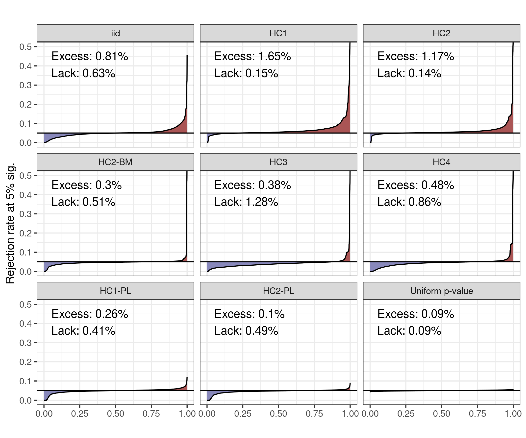
Figure 1: Main Results of Monte Carlo Study

Note: Each pane shows for a different specification of standard errors and degrees of freedom the distribution of rejection rate of t-tests with a 5% significance level across 3280 different regression coefficients from 608 regressions taken from 155 different reproduction packages. Red areas correspond to regression coefficients with excessive rejection rates (above 5%) and blue areas to those with lacking rejection rates (below 5%). For each specification the average excess and lack of the rejection rates across all regression coefficients is reported.

Figure 1 shows the results of large-scale Monte Carlo simulations based on 608 OLS regressions that have been originally estimated with heteroskedasticity-robust standard errors in 155 different reproduction packages of articles published in leading economic journals. Only regressions with a sample size $n$ below 1000 observations are considered. Appendix A provides details on the sample selection criteria and also shows descriptive statistics on the usage of different types of standard errors using static code analysis of 4650 reproduction packages.

For each original regression of the form

$$y^{o}=X\beta^{o}+\varepsilon^{o},$$

we specify a custom data generating process

$$y=X\beta+\varepsilon$$

with the same $n\times K$ matrix of explanatory variables $X$ as in the original regression. The true coefficients, $\beta$, are set to zero, and the error terms, $\varepsilon$, are assumed to satisfy $\varepsilon_{i}\sim N(0,\sigma_{i}^{2})$ for each observation $i=1,\ldots,n$. In this setup, the standard deviation $\sigma_{i}$ of the error term $\varepsilon_{i}$ is specified using a random forest FGLS specification, which is estimated separately for each original regression. Further details on this procedure are provided in Appendix B.

For each original regression, we draw $M=10000$ Monte Carlo samples and compute the p-values for a t-test of the null hypothesis $\beta_{k}=0$ for up to 25 coefficients, $\beta_{k}$, per regression. Each of the 3280 tested coefficients from the 608 original regressions constitutes a distinct test situation, indexed by $s$.

For each test situation, we compare different specifications $\tau\in\{\text{IID, HC1, HC2, $\ldots$}\}$, which vary by the type of standard error and the specification of the degrees of freedom used in the t-distribution. A refresher on the different types of robust standard errors is provided in Section 3. Let $p_{\tau,s}(m)$ denote the realized p-value for Monte Carlo sample $m=1,\ldots,M$ in specification $\tau$ and test situation $s$. Our analysis focuses on the 5% significance level. The simulated rejection rate is defined as the proportion of Monte Carlo samples for which the p-value is below 0.05:

$$\pi_{\tau,s}^{0.05}=\frac{1}{M}\sum_{m=1}^{M}I(p_{\tau,s}(m)\leq 0.05)$$

where $I(\cdot)$ is the indicator function. Since the null hypothesis is true in all test situations, p-values should be uniformly distributed under a correctly specified t-test. Consequently, the ideal value of the rejection rate $\pi_{\tau,s}^{0.05}$ is 0.05.

We measure deviations from this ideal value using the excess and lack of the rejection rate, defined as:

$$\text{excess}_{\tau,s}=\max\left(\pi_{\tau,s}^{0.05}-0.05,0\right),$$

$$\text{lack}_{\tau,s}=\max\left(0.05-\pi_{\tau,s}^{0.05},0\right).$$

While an excessive rejection rate increases the risk of false discoveries, lack in rejection rates can lead to under-powered significance tests. Excess is generally regarded as more problematic than an equally high lack. However, opinions may differ regarding acceptable levels of excess and the degree of lack one is willing to tolerate for a given reduction in excess.

Figure 1 reports, for each specification $\tau$, the average excess and lack across all 3280 test situations. Consistent with conventional wisdom, average excess decreases when moving in order from HC1, HC2, HC4, to HC3 standard errors, while average lack correspondingly increases.

Surprisingly, in our sample of regressions with no more than 1000 observations, i.i.d. standard errors, which are consistent only under homoskedasticity, are more conservative on average, in terms of lower excess, than both HC1 and HC2 standard errors. The HC2-BM specification corresponds to HC2 standard errors with an alternative degrees-of-freedom adjustment for the $t$-test proposed by Bell and McCaffrey (2002) and Imbens and Kolesár (2016).

Hereafter, we say that one specification outperforms another on average if it has a lower weighted sum of average excess and average lack, assuming the weight on excess is at least as large as the weight on lack. By this criterion, HC2-BM outperforms HC1, HC2, HC3, and HC4 on average. This result underscores the importance of correctly specifying degrees of freedom.

The HC1-PL and HC2-PL specifications employ a novel approach based on partial leverages to determine degrees of freedom, as detailed in Section 2. Both specifications outperform all others on average, with HC2-PL outperforming HC1-PL.

The last pane in Figure 1 corresponds to a simulated ideal case where the $p$-values of all $t$-tests are uniformly distributed. Reflecting the finite number of Monte Carlo samples, there is positive average excess and lack, both around 0.09%. While the average excess of HC2-PL closely approaches this ideal case, its average lack remains more than five times higher.

In addition to average excess and lack, one may also be interested in the distribution of excess and lack across test situations. Each pane of Figure 1 displays the rejection rates $\pi_{\tau,s}^{0.05}$ of all 3280 test situations, arranged in increasing order with the quantile level on the x-axis. Blue and red shaded areas represent rejection rates $\pi_{\tau,s}^{0.05}$ associated with positive lack and excess, respectively. The average lack and excess for specification $\tau$ correspond to the total size of the respective blue and red areas.

No specification $\tau$ exhibits uniformly excessive or uniformly lacking rejection rates across all test situations. As shown on the left-hand side of each pane, all specifications have rejection rates close to zero in some test situations. Conversely, except for HC1-PL and HC2-PL, all specifications include a few test situations with extremely high rejection rates exceeding 50%.

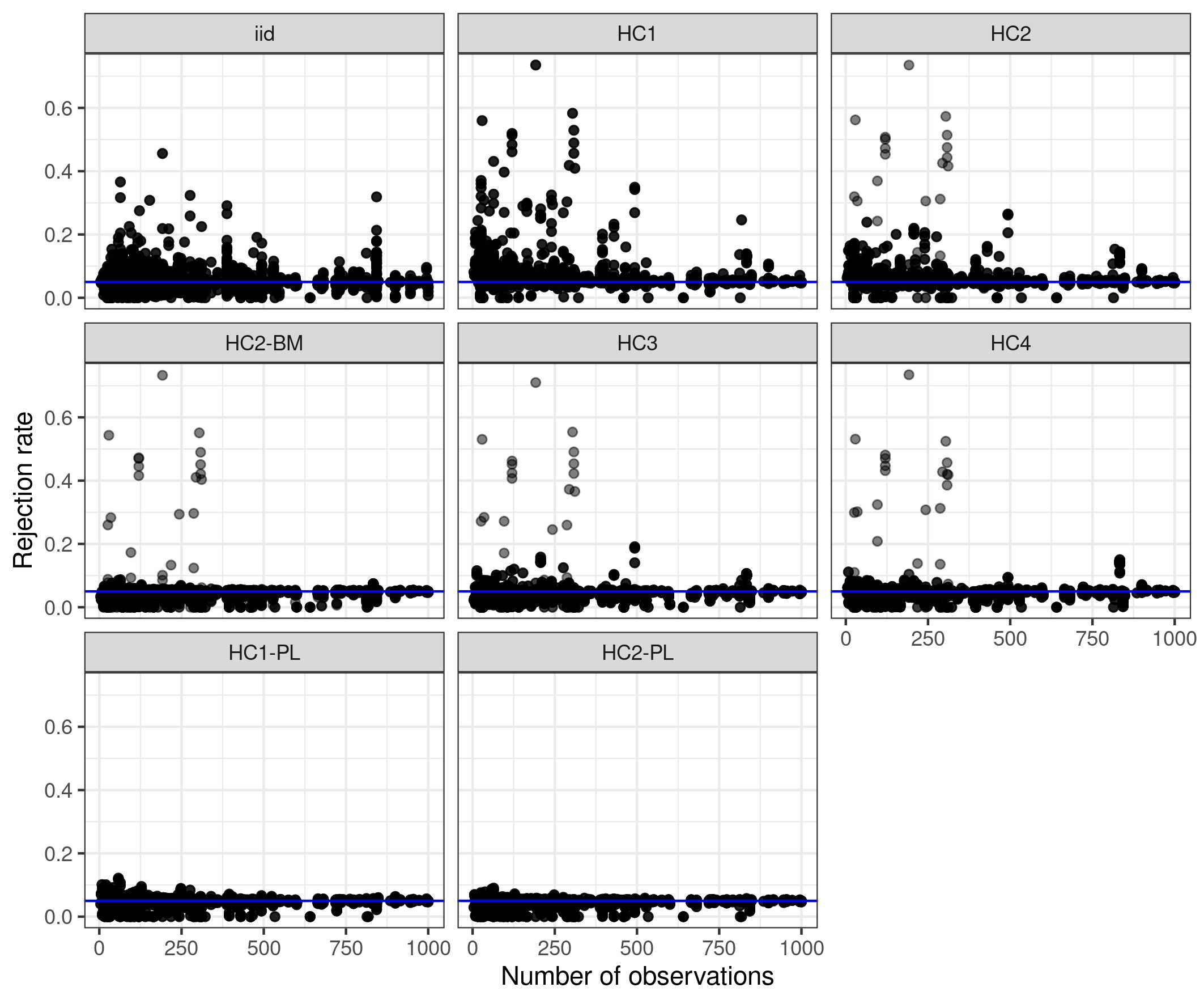
Figure 2: Rejection rates against sample size

Figure 2 plots the rejection rates against the sample size of each test situation. While highly excessive rejection rates are more likely for smaller sample sizes, we find them also in test situations with moderate sample sizes.

Section 2 shows that highly excessive rejection rates are characterized by highly concentrated partial leverages and introduces specifications HC1-PL and HC2-PL as a remedy. Section 3 provides a deeper exploration of HC1 to HC4 standard errors and shows that inference can be improved by an alternative handling of regressions that have at least one observation with leverage 1. Section 4 briefly concludes with additional observations, like the extension of some insights to cluster robust standard errors.

Due to the significant computational demands, wild bootstrap methods are analyzed for only a subset of test situation, with the corresponding results presented in Appendix C. While wild bootstrap specifications outperform the conventional HC1 and HC2 specifications, they are outperformed by the HC2-BM, HC1-PL, and HC2-PL specifications that utilize customized degrees of freedom.

2 Specifying Degrees of Freedom with Partial Leverages

Various diagnostics have been proposed to ensure robust inference. One recommendation by MacKinnon et al. (2023b) is to report partial leverages. Consider the linear regression model:

$$y=X\beta+\varepsilon,$$ (1)

where $y$ is the dependent variable, $X$ is the matrix of explanatory variables, $\beta$ is the vector of coefficients, and $\varepsilon$ represents the error term.

Using the Frisch-Waugh-Lovell (FWL) theorem, coefficient $\beta_{k}$ can be estimated with the simpler model:

$$\tilde{y}_{k}=\beta_{k}\tilde{x}_{k}+\tilde{\varepsilon}_{k},$$ (2)

where $\tilde{y}_{k}$ and $\tilde{x}_{k}$ are the residuals from regressing $y$ and $x_{k}$, respectively, on all other explanatory variables in $X$ except for $x_{k}$. Estimation of model (2) yields the same OLS residuals $\hat{\varepsilon}$ and estimator $\hat{\beta}_{k}$ as the original model (1).

The partial leverage for observation $i$ with respect to explanatory variable $x_{k}$ is defined as:

$$\tilde{h}_{k,i}=\frac{\tilde{x}_{k,i}^{2}}{\sum_{j=1}^{n}\tilde{x}_{k,j}^{2}},$$ (3)

where $\tilde{x}_{k,i}$ is the $i$-th element of $\tilde{x}_{k}$.

Partial leverages satisfy $0\leq\tilde{h}_{k,i}\leq 1$ and $\sum_{i=1}^{n}\tilde{h}_{k,i}=1$. Furthermore, for $n\geq 2$, we have $\tilde{h}_{k,i}<1$ if the original regression model includes a constant.

To build intuition, consider an example where partial leverages are highly concentrated. Let $x_{k}$ be a dummy variable such that $x_{1,k}=1$ and $x_{i,k}=0$ for all $i=2,\ldots,n$. Assume $x_{k}$ is uncorrelated with other explanatory variables. As the sample size $n$ grows, the partial leverage of the first observation $\tilde{h}_{k,1}$ converges to 1.

More intuition about partial leverages can be gained by reformulating the OLS estimator as follows:

$$\hat{\beta}_{k}=\beta_{k}+\frac{\sum_{i=1}^{n}\sqrt{\tilde{h}_{k,i}}\,\tilde{\varepsilon}_{k,i}}{\sqrt{\sum_{i=1}^{n}\tilde{x}_{k,i}^{2}}}.$$ (4)

We see that in the aforementioned example, where the partial leverage is concentrated on observation $i=1$, the variation in $\hat{\beta}_{k}$ will be predominantly driven by the realization of $\tilde{\varepsilon}_{1}$. If high concentrations of partial leverage are not adequately accounted for in $t$-tests, the resulting rejection probabilities may deviate substantially from their nominal levels.

A widely used concentration measure in competition policy is the Herfindahl-Hirschman index, defined as the sum of the squared market shares of all competitors in a market. Analogously, in our context, the concentration of partial leverages can be measured by the sum of squared partial leverages. We denote the inverse of this measure as:

$$\tilde{n}_{k}=\left(\sum_{i=1}^{n}\tilde{h}_{k,i}^{2}\right)^{-1}$$ (5)

We refer to $\tilde{n}_{k}$ as the partial-leverage-adjusted sample size. It satisfies $1\leq\tilde{n}_{k}\leq n$. If all observations have the same partial leverage then $\tilde{n}_{k}=n$ and in the limit case that the partial leverage becomes concentrated in a single observation $\tilde{n}_{k}\rightarrow 1$.

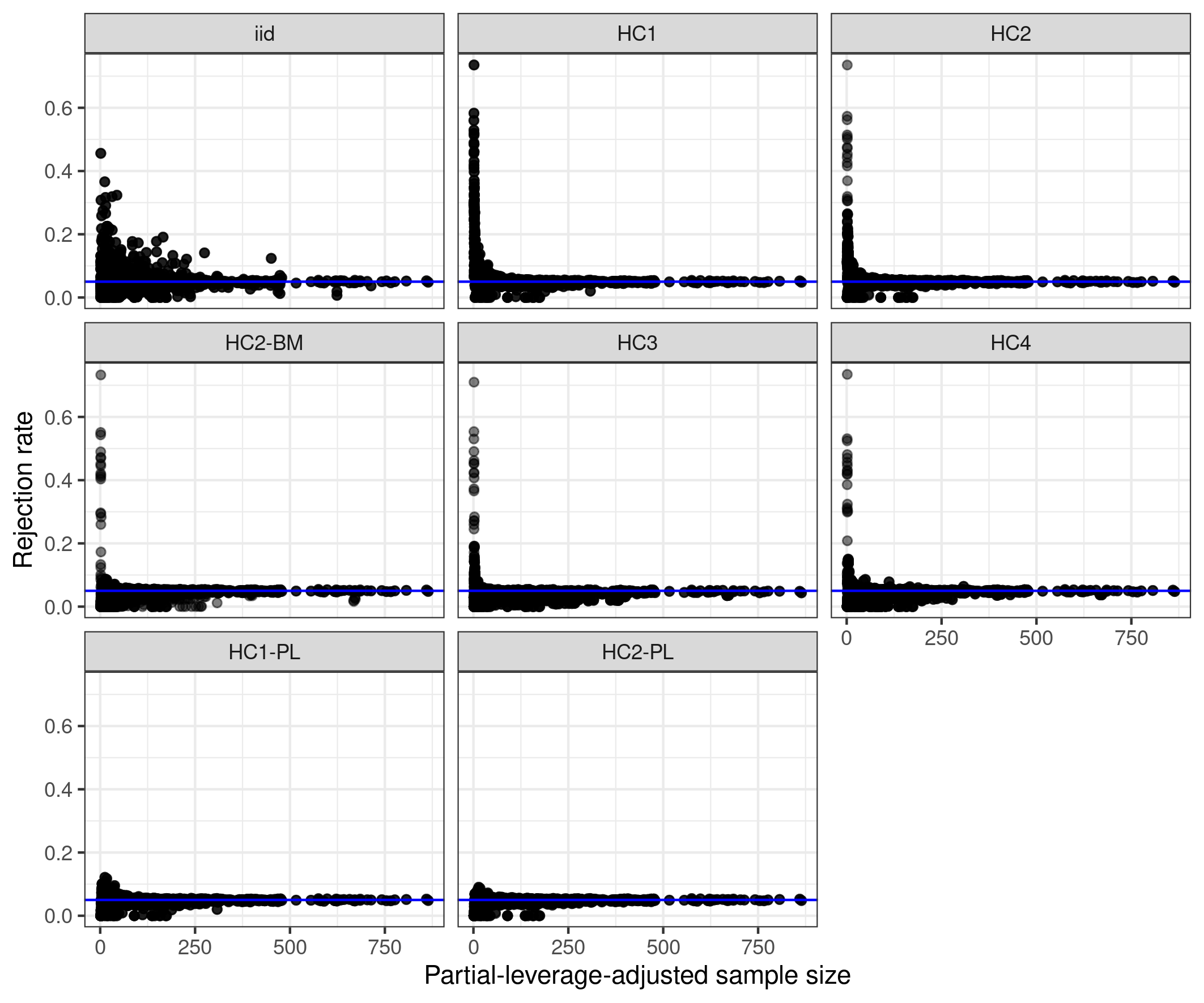
Figure 3: Rejection rates against partial-leverage-adjusted sample sizes

Figure 3 illustrates a clear pattern for standard errors HC1 through HC4, as well as for specification HC2-BM: all test situations with highly excessive rejection rates exhibit very small partial-leverage-adjusted sample sizes. This observation motivates our novel specifications: HC1-PL and HC2-PL. These methods specify the degrees of freedom in the $t$-test as $\tilde{n}_{k}-1$ and use HC1 and HC2, respectively, as standard errors.

To understand why we specify the degrees of freedom as $\tilde{n}_{k}-1$ instead of $\tilde{n}_{k}$, consider the following. As long as the original sample contains at least two observations, we have $\tilde{n}_{k}>1$. Since a $t$-distribution can be defined for any fractional degrees of freedom strictly greater than zero, this adjustment ensures properly defined degrees of freedom whenever $n\geq 2$. In the degenerate case of a single observation, no standard error can be computed, and the corresponding $t$-distribution with zero degrees of freedom becomes degenerate. Using $\tilde{n}_{k}-1$ as the degrees of freedom allows for continuous convergence to this degenerate case as $\tilde{n}_{k}\to 1$.

Moreover, non-reported Monte Carlo results suggest that the specifications using $\tilde{n}_{k}-1$ perform substantially better in test situations with low values of $\tilde{n}_{k}$.

Appendix D provides an additional justification for the partial-leverage-based degree of freedom adjustment by deriving it from a Satterthwaite approximation, similar to the approach of Bell and McCaffrey (2002).

3 Specification of Robust Standard Errors and Dealing with Leverage of One

This section provides additional insights into the role of leverage, complementing the previous findings on partial leverage. We first present the mathematical formulations of robust standard errors HC0 to HC4. Consider the linear regression model:

$$y=X\beta+\varepsilon,$$

where the error terms $\varepsilon_{i}$ are independently distributed with mean zero and variance $\sigma_{i}^{2}$. The true variance-covariance matrix of $\hat{\beta}$ is given by:

$$\text{Var}(\hat{\beta})=(X^{\top}X)^{-1}\left(\sum_{i=1}^{n}\sigma_{i}^{2}x_{i}x_{i}^{\top}\right)(X^{\top}X)^{-1},$$

where $x_{i}$ denotes the $i$-th row of $X$.

Heteroskedasticity-robust variance estimators of types HC0 to HC4 can all be expressed in the general form:

$$\hat{V}^{\tau}(\hat{\beta})=(X^{\top}X)^{-1}\left(\sum_{i=1}^{n}\alpha_{i}^{\tau}\hat{\varepsilon}_{i}^{2}x_{i}x_{i}^{\top}\right)(X^{\top}X)^{-1},$$

where $\hat{\varepsilon}_{i}$ is the OLS residual for observation $i$, and $\alpha_{i}^{\tau}$ is an adjustment factor that depends on the specification $\tau$. The corresponding standard errors are obtained as the square roots of the diagonal elements of $\hat{V}^{\tau}(\hat{\beta})$.

The HC0 estimator, developed by Eicker (1967), Huber (1967), and White (1980), sets $\alpha_{i}^{HC0}=1$. While consistent, HC0 can exhibit severe bias in small samples and is rarely used in practice. MacKinnon and White (1985) introduced three variants, HC1, HC2 and HC3, with improved small-sample properties.

The HC1 adjustment factor is:

$$\alpha_{i}^{HC1}=\frac{n}{n-K}.$$

This correction mirrors the degrees of freedom adjustment used in the unbiased estimator $\hat{\sigma}^{2}=\frac{1}{n-K}\sum_{i=1}^{n}\hat{\varepsilon}_{i}^{2}$ for the error variance $\sigma^{2}=E[\varepsilon_{i}^{2}]$ under homoskedasticity.

The HC2 adjustment factor is given by:

$$\alpha_{i}^{HC2}=\frac{1}{1-h_{i}},$$

where $h_{i}$ is the leverage of observation $i$, defined as the $i$-th diagonal element of the hat matrix:

$$H=X(X^{\top}X)^{-1}X^{\top}.$$

Leverages satisfy $0\leq h_{i}\leq 1$ and $\sum_{i=1}^{n}h_{i}=K$. We address the special case where an observation $i$ has $h_{i}=1$ further below. HC2 can be motivated by the property that, under homoskedasticity, $E[\hat{\varepsilon}_{i}^{2}]=(1-h_{i})\sigma^{2}$. Furthermore, in the homoskedastic case, $\hat{V}^{HC2}(\hat{\beta})$ is an unbiased estimator of $\text{Var}(\hat{\beta})$.

The HC3 adjustment factor is also based on leverages:

$$\alpha_{i}^{HC3}=\frac{1}{(1-h_{i})^{2}}.$$

As shown in Hansen (2022), HC3-adjusted residuals $\sqrt{\alpha_{i}^{HC3}}\hat{\varepsilon}_{i}$ are equivalent to the leave-one-out prediction error $y_{i}-x_{i}\hat{\beta}_{(i)}$, where $\hat{\beta}_{(i)}$ denotes the OLS estimator obtained from the regression excluding observation $i$. The HC3 estimator can also be interpreted as a jackknife estimator, satisfying

$$\hat{V}^{HC3}(\hat{\beta})=\sum_{i=1}^{N}(\hat{\beta}_{(i)}-\hat{\beta})(\hat{\beta}_{(i)}-\hat{\beta})^{\top}.$$

The HC4 estimator, introduced by Cribari-Neto (2004), aims to better handle cases with high leverages by modifying the adjustment factor to:

$$\alpha_{i}^{HC4}=\frac{1}{(1-h_{i})^{\delta}},$$

where $\delta_{i}=\min\left\{4,\frac{nh_{i}}{K}\right\}$.

Following common practice, we use $n-K$ degrees of freedom in $t$-tests based on HC1 to HC4 standard errors.

The specification HC2-BM combines HC2 standard errors with a degree of freedom adjustment proposed by Bell and McCaffrey (2002) based on an approximation suggested by Satterthwaite (1946). See Imbens and Kolesár (2016) for further exploration of this adjustment. Appendix D provides a similar motivation for the novel degrees of freedom adjustments used in HC1-PL and HC2-PL.

15.6% of the regressions in our replication sample include at least one observation with $h_{i}=1$. In such cases, the formulas for HC2, HC3, and HC4 variance estimators are not well-defined. Specifically, if $h_{i}=1$, the corresponding OLS residual $\hat{\varepsilon}_{i}$ is exactly zero, and $\alpha_{i}^{\tau}\hat{\varepsilon}_{i}^{2}$ involves the mathematically indeterminate form $0/0$. A similar issue arises in the context of cluster-robust standard errors. Pustejovsky and Tipton (2017) theoretically justify using a generalized Moore-Penrose inverse, which Kolesár (2023) adapts for HC2 heteroskedasticity-robust standard errors. The Moore-Penrose inverse of $1-h_{i}$ for $h_{i}=1$ is zero, implying that $\alpha_{i}^{\tau}\hat{\varepsilon}_{i}^{2}$ is set to zero for observations with $h_{i}=1$. Pötscher and Preinerstorfer (2023) adopt this convention for HC3 and HC4 as well. We follow this approach in our Monte Carlo study presented in Section 1.

However, this handling of $h_{i}=1$ is not universal. For instance, the sandwich package in R (Zeileis, 2004) returns no value for standard errors (NaN) if there is an observation with $h_{i}=1$. Stata’s approach is not yet well-documented, but experiments and personal communications suggest that if $h_{i}=1$, Stata evaluates $\alpha_{i}^{\tau}\hat{\varepsilon}_{i}^{2}=0/0$ numerically, which yields a result determined by rounding errors.

Let $h_{\text{max}}=\max_{i=1,\ldots,n}h_{i}$ denote the maximum leverage across all observations. Figure 4 plots rejection rates against $h_{\text{max}}$ for each specification.

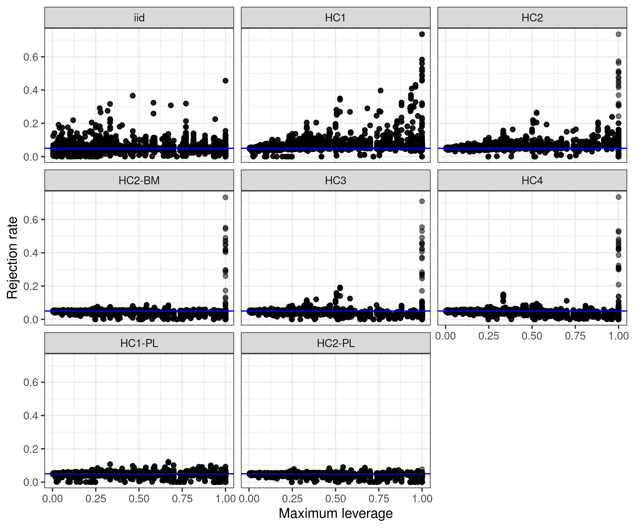
Figure 4: Rejection rates against maximum leverage $h_{max}$

The results show that test situations with highly excessive rejection rates for HC1 to HC4 are mostly characterized by very high $h_{\text{max}}$. In particular, for HC2-BM, and to a lesser extent for HC3 and HC4, cases of extremely excessive rejection rates almost exclusively occur when $h_{\text{max}}=1$. For HC1 and HC2, some fairly excessive rejection rates are observed even for lower values of $h_{\text{max}}$. Overall, a small partial-leverage-adjusted sample size $\tilde{n}_{k}$ and high maximum leverage $h_{\text{max}}$ indicate similar problems in rejection rates. The relationship between rejection rates and $\tilde{n}_{k}$ appears slightly clearer, though.

Figure 4 further suggests that the HC1-PL and HC2-PL specifications, which use $\tilde{n}_{k}-1$ degrees of freedom in the $t$-test, exhibit almost no systematic relationship between rejection rates and $h_{\text{max}}$. Thus, if concentrated partial leverages are appropriately accounted for, inference appears to be robust even in the presence of large leverages.

Yet, for specifications other than HC1-PL and HC2-PL an alternative treatment for cases where $h_{i}=1$ may yield improvements. Instead of setting $\alpha_{i}^{\tau}\hat{\varepsilon}_{i}^{2}=0$, it seems natural to omit all observations with $h_{i}=1$ entirely when computing standard errors. This approach also excludes those observations from the computation of $(X^{\top}X)^{-1}$. Figure 5 compares this treatment with the treatment of setting $\alpha_{i}^{\tau}\hat{\varepsilon}_{i}^{2}$ equal to zero if $h_{i}=0$.

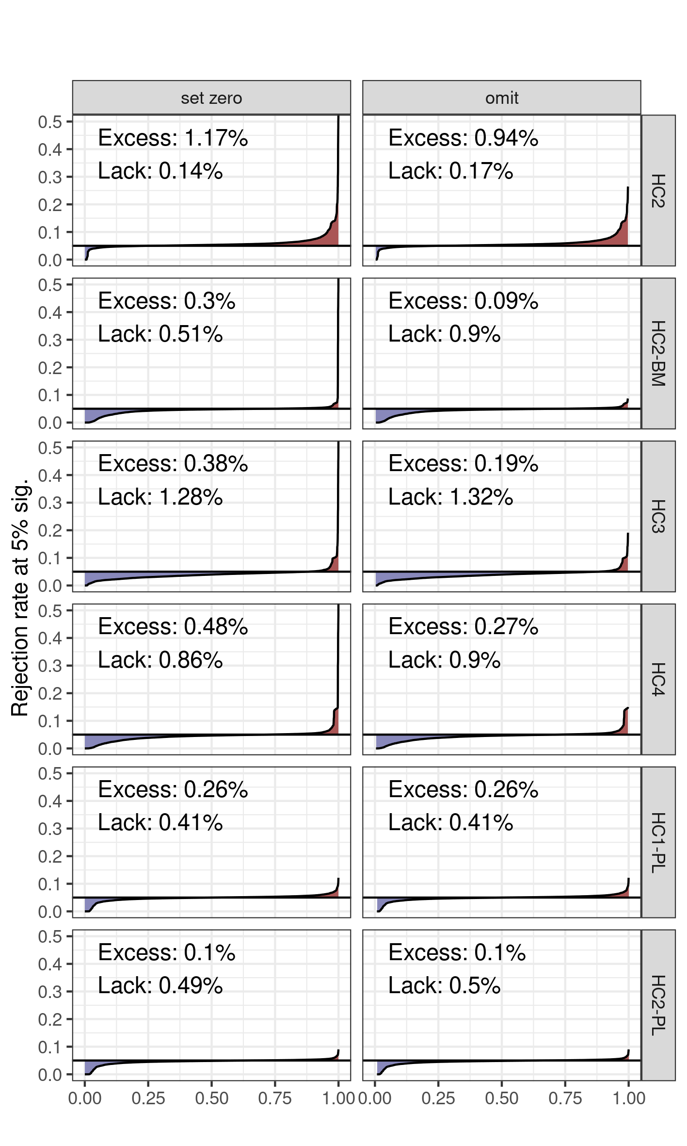
Figure 5: Comparing rejection rates for two different treatments of cases with $h_{i}=1$

Completely omiting observations with $h_{i}=1$ reduces average excess across all traditional specifications and also instances of extremely high excess are either completely removed or substantially reduced. There is also no longer a clear ranking between HC2-BM and HC2-PL. For HC1-PL and HC2-PL the treatment of cases with $h_{i}=1$ has little effect on the rejection rates.

Our overall recommendation for heteroskedastic robust inference is thus the following: either compute degrees of freedom using the adjustment based on partial-leverages used in specifications HC1-PL or HC2-PL, or apply a modified version of the Bell & McCaffrey (2002) procedure that completely omits observations with $h_{i}=1$.

4 Concluding Remarks

Our proposed degree of freedom adjustment can be directly applied to compute confidence intervals. Moreoever, following the approach of Imbens and Kolesár (2016), one could report adjusted standard errors by multiplying the original standard errors with $q_{\tilde{n}_{k}-1}^{t}(0.975)/q_{n-K}^{t}(0.975)$ where $q_{\nu}^{t}$ is the quantile function of the t-distribution with $\nu$ degreess of freedom.

Since partial leverages are defined for a single explanatory variable $x_{k}$ only, it is not obvious how the corresponding degrees of freedom adjustment can be extended to hypothesis tests involving multiple coefficients. In contrast, the degree of freedom formula proposed by Bell and McCaffrey (2002) does not face this limitation.

In our Monte Carlo studies, HC1-PL was surprisingly close behind the performance of HC2-PL. The reghdfe Stata command (Correia, 2017) and the fixest R package (Berge, 2018), which are widely used for fixed effects regressions, provide heteroskedasticity-robust standard errors based solely on HC1. This is likely because extending the performance gains from fixed-effects absorption to the computation of hat values required for HC2-, HC3-, or HC4-based standard errors is non-trivial. In contrast, absorbed fixed effects do not pose any challenges for computing partial leverages and HC1 standard errors. Therefore, HC1-PL might be a promising alternative specification for regressions with absorbed fixed effects.

This paper does not perform Monte Carlo analysis for the robust inference methods proposed by Cattaneo et al. (2018) and by Pötscher, B. M., & Preinerstorfer, D. (2023). My limited econometric expertise feels insufficient to assess whether and how a sufficiently fast implementation for comprehensive Monte Carlo studies could be achieved. I hope that once the repbox toolbox is fully developed and documented, it will facilitate such studies by more skilled researchers in the future.

The introduced degree of freedom adjustment of HC1-PL and HC2-PL can be readily extended to cluster-robust inference. The partial leverage of cluster $g$ is defined as the sum of the partial leverages of all observations within cluster $g$. The inverse Herfindahl-Hirschman index is then computed by treating each cluster as a single observation, yielding a partial-leverage-adjusted number of clusters, $\tilde{G}_{k}$. A comprehensive Monte Carlo assessment for cluster-robust inference is planned for a separate paper.

Bibliography

• Athey, S., Tibshirani, J., & Wager, S. (2019). “Generalized random forests”. The Annals of Statistics, 47(2), 1148.

• Bell, R. M., & McCaffrey, D. F. (2002). “Bias reduction in standard errors for linear regression with multi-stage samples”. Survey Methodology, 28(2), 169-182.

• Berge L (2018). “Efficient estimation of maximum likelihood models with multiple fixed-effects: the R package FENmlm”. CREA Discussion Papers.

• Cattaneo, M. D., M. Jansson, and W. K. Newey. 2018. “Inference in linear regression models with many covariates and heteroscedasticity”. Journal of the American Statistical Association 113: 1350–1361.

• Chesher, A., and I. Jewitt. 1987. “The bias of a heteroskedasticity consistent covariance matrix estimator”. Econometrica 55: 1217–1222.

• Chesher, A., and G. Austin. 1991. “The finite-sample distributions of heteroskedasticity robust Wald statistics”. Journal of Econometrics 47: 153–173.

• Correia, Sergio. 2017. “Linear Models with High-Dimensional Fixed Effects: An Efficient and Feasible Estimator”. Working Paper. http://scorreia.com/research/hdfe.pdf

• Cribari-Neto, F. (2004). “Asymptotic inference under heteroskedasticity of unknown form”. Computational Statistics & Data Analysis, 45(2), 215-233.

• Christensen, Rune Haubo B (2018), “Satterthwaite’s Method for Degrees of Freedom in Linear Mixed Models”. Notes for the R package lmerTestR

• Davidson, R., & MacKinnon, J. G. (1993). “Econometric Theory and Methods”. Oxford University Press

• Ding, P. (2021). “The Frisch–Waugh–Lovell theorem for standard errors”. Statistics & Probability Letters, 168, 108945.

• Eicker, Friedhelm (1967). “Limit Theorems for Regression with Unequal and Dependent Errors”. Proceedings of the Fifth Berkeley Symposium on Mathematical Statistics and Probability. Vol. 5. pp. 59–82.

• Hansen, B. (2022). “Econometrics”. Princeton University Press.

• Huber, Peter J. (1967). "The behavior of maximum likelihood estimates under nonstandard conditions". Proceedings of the Fifth Berkeley Symposium on Mathematical Statistics and Probability. Vol. 5. pp. 221–233.

• Imbens, G. W., & Kolesár, M. (2016). “Robust standard errors in small samples: Some practical advice”. Review of Economics and Statistics, 98(4), 701-712.

• Kolesár, M. (2023), “Robust Standard Errors in Small Samples”. Vignette of the R package dfadjust.

• Pötscher, B. M., & Preinerstorfer, D. (2023). “Valid Heteroskedasticity Robust Testing”. Econometric Theory, 1–53.

• Pustejovsky, J. E., & Tipton, E. (2017). “Small-Sample Methods for Cluster-Robust Variance Estimation and Hypothesis Testing in Fixed Effects Models”. Journal of Business & Economic Statistics, 36(4), 672–683.

• MacKinnon, James G.; White, Halbert (1985). “Some Heteroskedastic-Consistent Covariance Matrix Estimators with Improved Finite Sample Properties”. Journal of Econometrics. 29 (3): 305–325.

• MacKinnon, J. G., Nielsen, M. Ø., & Webb, M. D. (2023a). “Fast and reliable jackknife and bootstrap methods for cluster-robust inference”. Journal of Applied Econometrics, 38(5), 671-694.

• MacKinnon, J. G., Nielsen, M. Ø., & Webb, M. D. (2023b). “Leverage, influence, and the jackknife in clustered regression models: Reliable inference using summclust”. The Stata Journal, 23(4), 942-982.

• Roodman, D., Nielsen, M. Ø., MacKinnon, J. G., & Webb, M. D. (2019). “Fast and wild: Bootstrap inference in Stata using boottest”. The Stata Journal, 19(1), 4-60.

• Satterthwaite, F. E. (1946), “An Approximate Distribution of Estimates of Variance Components,” Biometrics Bulletin 2, 110–114.

• White, Halbert (1980). “A Heteroskedasticity-Consistent Covariance Matrix Estimator and a Direct Test for Heteroskedasticity”. Econometrica. 48 (4): 817–838.

• Wu, C. F. J. (1986). “Jackknife, bootstrap and other resampling methods in regression analysis”. the Annals of Statistics, 14(4), 1261-1295.

• Young, A. (2019). “Channeling fisher: Randomization tests and the statistical insignificance of seemingly significant experimental results”. The Quarterly Journal of Economics, 134(2), 557-598.

• Young, A. (2022). “Consistency without inference: Instrumental variables in practical application”. European Economic Review, 147, 104-112.

• Zeileis, A. (2004). “Econometric Computing with HC and HAC Covariance Matrix Estimators”. Journal of Statistical Software, 11(10), 1–17.

Appendix A: Standard errors used in reproduction packages and selection of test situations for Monte Carlo studies

We base our code analysis on 4650 reproduction packages containing Stata scripts from articles published in leading economic journals. We utilize a custom-designed parser to systematically extract information from all code lines in the Stata scripts, with particular emphasis on lines containing regression commands.

Table A1 reports the frequency of the 10 most common regression commands identified in our sample.

Table A1: Top 10 of most used Stata regression commands

Regression command	No. reproduction packages	No. code lines
regress	3866	146847
areg	1416	41373
xtreg	859	19333
reghdfe	763	29921
ivregress	589	11975
ivreg2	498	11016
probit	474	4913
logit	371	3810
xtivreg2	213	5539
dprobit	165	2200

We restrict our analysis to OLS regressions performed using one of the following Stata commands: regress, areg, xtreg, or reghdfe. These commands appear in a total of 240615 code lines across 4420 reproduction packages. Table A2 provides a detailed breakdown of their distribution across journals.

Table A2: Numbers of reproduction packages and regression commands by journal

Journal	Reproduction packages	Regression commands
aer	1085	57834
aejapp	552	37463
aejpol	503	31741
restat	497	25838
pandp	244	3026
ms	241	12600
aejmac	202	13052
restud	169	9822
jpe	152	9971
jole	143	9079
jeea	135	8069
aejmic	104	3004
ecta	92	5609
jep	86	2533
aeri	73	2749
qje	72	5305
jaere	70	2920
Total	4420	240615

The standard errors used in these regressions fall into three main categories: 17.1% heteroskedasticity-robust, 61% cluster-robust, and 21.6% homoskedastic. Panel A of Table 1 reports the absolute numbers for each category.

Table A3: Static Code Analysis: Frequency of Standard Errors

	No. reproduction packages	No. code lines
Panel A: Standard error category
cluster	3055	144882
iid	2937	51230
robust	1689	40571
unknown	47	791
Panel B: Type of heteroskedasticity robust standard error
hc1	1660	39782
bootstrap	54	765
hc3	3	24

For simplicity, we will often refer to heteroskedasticity-robust standard errors as robust standard errors. Panel B of Figure 1 illustrates the frequency of specific types of robust standard errors: 98.1% of regression commands use Stata’s default robust standard error, HC1. This finding suggests that common recommendations, see, for example, MacKinnon and White (1985), Chesher and Jewitt (1987), Chesher and Austin (1991), Long and Ervin (2000), or Cattaneo, Jansson, and Newey (2018), to adopt more robust alternatives in smaller samples, such as HC3, are rarely followed.

From the reproduction packages containing an OLS regression with robust standard errors, we select the underlying regressions for the Monte Carlo study based on the following criteria:

• The size of the reproduction package’s ZIP file is below 10 MB.

• The regression command can be successfully run. The most common cause of a run error is the absence of confidential or proprietary data sets in the reproduction packages.

• A successful run of an automatic translation of the regression to R, based on the extracted information about the original regression. The second run must yield the same results as the original Stata run, except for small numerical discrepancies.

• The entire reproduction, including the extraction and storage of regression related information and the 2nd reproduction run in R for all regressions, takes less than 15 minutes for the whole reproduction package. Reproduction runs that take longer are currently cancelled with a timeout.

• From each reproduction package with regressions meeting these criteria, at most four regressions are selected for the Monte Carlo simulations.

• For each regression, $t$-tests are performed on at most 25 regression coefficients. Each regression is estimated with a Least Squares Dummy Variable (LSDV) specification, even if the original Stata command uses absorbed fixed effects, to enable the computation of proper HC2, HC3, and HC4 standard errors. $t$-tests are not performed for originally absorbed fixed effects. Additionally, heuristics are used to identify dummy variable sets that are not absorbed but look like fixed effects. For these dummy variables no t-tests are performed either.

It is somewhat disappointing that we currently end up with only 155 reproduction packages containing at least one regression that satisfies all the criteria above. While some issues, such as missing data in a reproduction package, cannot be resolved, there remain additional points of failure in the process of reproducing the original Stata regression in R.

As noted in the inital footnote, I develop a general toolbox named repbox in R to facilitate meta studies like the current one. Repbox does not only help to translate regression commands to R but also attempts to store the datasets used in the regressions in a manner that allows the data preparation steps to be automatically performed in R. This step is complex and provides another point of potential failure.

Still, the 155  reproduction packages used as the basis for our Monte Carlo studies substantially exceed the scale of similar studies in economics that we are aware of. For example, the large-scale study by Young (2019) hand-collected reproducible regressions from 53 economic articles with experimental studies, while Young (2022) conducted large-scale Monte Carlo studies based on instrumental variables regressions from 30 economic articles.

The number of test situations could be easily increased by selecting more than the current maximum of four regressions from each reproduction package. However, this approach risks skewing the results, as they may become more strongly influenced by a smaller number of reproduction packages that contain a large number of regressions.

Appendix B: Specifying DGPs for our Monte Carlo Studies

Assume the model of the original regression $r$ estimated in the reproduction package is given by

$$y^{r,o}=X\beta^{r,o}+\varepsilon^{r,o}.$$

The corresponding Monte Carlo samples will be generated from the model:

$$y^{r}=X\beta^{r}+\varepsilon^{r}.$$

The explanatory variables $X$ remain unchanged from the original sample and we set $\beta^{r}=0$. To determine the distribution of the error terms $\varepsilon^{r}$ for each Monte Carlo model, we use the following general procedure:

1. For each original regression $r$, we specify a set of $C$ candiate models $\mathcal{M}^{r,c}$ indexed by $c=1,...,C$ for the distribution of the error term. We only consider candidate models with independently distributed error terms for Monte Carlo sample $m$ satisfying $\varepsilon_{i}^{m,r,c}\sim N(0,\left(\sigma_{i}^{r,c}\right)^{2})$. This means each candidate model is fully characterized by the specified vector of standard errors $\sigma^{r,c}$ of the error term.

2. From each candidate model we draw $m=1,...,M$ samples of the error term $\varepsilon^{m,r,c}$ and compute the corresponding OLS residuals $\hat{\varepsilon}^{m,r,c}.$

3. We then compute for each candidate model a distance $d^{r,c}$ between the original OLS residuals $\hat{\varepsilon}^{r,o}$ and the set of Monte Carlo residuals $\{\hat{\varepsilon}^{m,r,c}\}_{m=1}^{M}$.

4. For each original regression $r$, we pick that candidate model for the Monte Carlo DGP that has the lowest distance $d^{r,c}$.

One candidate model assumes purely homoskedastic error terms, while all other candidate models estimate error term standard errors $\sigma_{i}^{r,c}$ using a non-parametric FGLS specification based on random forests. The dependent variable of the random forest is the absolute value of the original OLS residuals, $\left|\hat{\varepsilon}_{i}^{r,o}\right|$. The explanatory variables of the random forest are the same as the explanatory variables in the original regression. Compared to a feasible GLS specification based on a log-linear regression model, random forests offer greater flexibility and are well-suited to capture non-linear effects and interactions among explanatory variables in predicting heteroskedasticity. Since random forest predictions are always computed as averages of the dependent variable in the training dataset, they cannot produce negative standard errors.

Whether the random forest predicts larger or smaller degrees of heteroskedasticity (measured by the variation in $\sigma_{i}$) depends on how the random forest is trained and how predictions are performed. Ordered from typically larger to smaller predicted heteroskedasticity, we consider five different candidates: in-sample prediction, out-of-bag prediction, out-of-bag prediction based on honest trees (see Athey et al., 2019), an equally weighted linear combination of out-of-bag prediction for honest trees and a homoskedastic model, and a purely homoskedastic model.

No single approach provides the best fit for all original regression specifications. One indicator of the approximation quality is the similarity between the sample distribution of the original OLS residuals and the distribution of the Monte Carlo OLS residuals. To evaluate candidate models, we particularly focus on the kurtosis of the OLS residuals: if the original error terms are i.i.d. and normally distributed, the OLS residuals exhibit a kurtosis close to 3, whereas heteroskedasticity generally increases the kurtosis.

More formally, let $\kappa^{m,r,c}$ denote the kurtosis of the OLS residuals in Monte Carlo sample $m$ for candidate model $c$ of original regression $r$. Let $\bar{\kappa}^{r,c}$ and $s_{\kappa}^{r,c}$ denote the corresponding mean and standard deviation of the kurtoses across all $M$ Monte Carlo samples. A basic distance measure for candidate model $c$ for original regression $r$ is the standardized distance

$$\delta^{c,r}=\frac{\left|\bar{\kappa}^{r,c}-\kappa^{r,o}\right|}{s_{\kappa}^{r,c}}$$

where $\kappa^{r,o}$ is the kurtosis of the original OLS residuals. To some extent, this distance measure may favor data-generating processes that produce OLS samples with high variability in kurtosis. To counteract this effect, we also consider a modified distance measure:

$$\bar{\delta}^{c,r}=\frac{\left|\bar{\kappa}^{r,c}-\kappa^{r,o}\right|}{\bar{s}_{\kappa}^{r}}$$

where $\bar{s}_{\kappa}^{r}$ denotes the median of the kurtosis standard deviations across all candidate models for the original regression $r$. The final distance measure used is the average of these two measures:

$$d^{c,r}=0.5\delta^{c,r}+0.5\bar{\delta}^{c,r}$$

The chosen DGP for original regression $r$ is the candidate model $c$ with the lowest distance $d^{c,r}$.

We do not base the selection of DGP on the standard deviations of residuals. Instead, all candidate models are calibrated to produce OLS residuals with standard deviations similar to those of the original OLS residuals. This calibration is achieved by scaling the initially obtained values of $\sigma^{r,c}$ by the ratio of the standard deviations of the original residuals and the Monte Carlo residuals, $sd(\hat{\varepsilon}^{r,o})/sd(\hat{\varepsilon}^{m,r,c})$.

Appendix C: Wild Bootstrap Inference

Wild bootstrap techniques have gained a lot of attention in the context of cluster robust inference, see e.g. Roodman et al. (2019) and MacKinnon et al. (2023). For hetereoskedasticity-robust inference they have been proposed already by Wu (1986). We compute wild bootstrap p-values for the t-test with null hypothesis $\beta_{k}=0$ as follows:

1. Estimate the restricted regression model under the null hypothesis $\beta_{k}=0$ to obtain OLS residuals $e^{r}$ and predicted values $\hat{y}^{r}$.

2. Generate bootstrap error terms $\varepsilon^{b}=\sqrt{\alpha^{\theta}}e^{r}\cdot v^{b}$, where $\alpha^{\theta}$ is an adjustement based on type $\theta\in\{\text{HC1,HC2,HC3}\}$ as specified in Section 3. The factor $v^{b}$ is an $n\times 1$ vector of random weights independently drawn from a Rademacher distribution

   $$v_{i}^{b}=\begin{cases}-1&\text{with probability }0.5\\ 1&\text{with probability }0.5\end{cases}$$

3. Form a bootstrap sample $y^{b}=\hat{y}^{r}+\varepsilon^{b}$ and re-estimate the model to obtain the OLS estimator $\hat{\beta}_{k}^{b}$ and a corresponding variance estimator $\hat{V}_{k}^{b,\eta}$ of type $\eta\in\{\text{HC1,HC2,HC3}\}$. We then compute the corresponding t-statistic for the null hypothesis $\beta_{k}=0$:

   $$t_{k}^{b,\eta}=\frac{\hat{\beta}_{k}^{b}}{\sqrt{\hat{V}_{k}^{b,\eta}}}$$

4. Repeat steps 2 and for 3 for $B$ bootstrap replications to construct the bootstrap distribution of the test statistic.

5. Calculate the bootstrap p-value as the proportion of bootstrap statistics $t_{k}^{b,\eta}$ that are as extreme as or more extreme than the test statistic $t_{k}^{\eta}$ from the original regression sample (also computed using a standard error of type $\eta$):

   $$\text{p-value}=\frac{1}{B}\sum_{b=1}^{B}I(|t_{k}^{b,\eta}|\geq|t_{k}^{\eta}|),$$ (6)

   where $I(\cdot)$ is the indicator function.

We compare 9 different specifications $\tau\in\{\text{WB-11,WB-21},...,\text{WB-33\}}$ of wild bootstrap p-values, one for each combination $(\theta,\eta)\in\{\text{HC1,HC2,HC3}\}\times\{\text{HC1,HC2,HC3}\}$.

Similar to the previous Monte Carlo analysis we evaluate for each original regression $M=10000$ Monte Carlo samples and we draw $B$ separate wild bootstrap samples for each Monte Carlo sample $m$. Ideally, we would prefer to set $B$ to a large value in order to precisely estimate bootstrap p-values for each Monte Carlo sample. However, this approach presents a practical challenge. While wild bootstrap p-values can be computed significantly faster than those based on the paired bootstrap, the combination of a large $M$ and $B$, together with over a thousand test situations, renders the computational burden of the Monte Carlo study infeasible within acceptable time frames given the limitations of our hardware.

We first derive a theoretical result that suggests that the rejection rate $\pi_{\tau,s}^{0.05}$ for wild bootstrap methods can already be well approximated with a smaller number of bootstrap repetitions. Let $p_{\tau,s|B}(m)$ denote the bootstrap p-value for Monte Carlo sample $m$ computed with $B$ bootstrap repetitions and let

$$\pi_{\tau,s|B}^{0.05}=\frac{1}{M}\sum_{m=1}^{M}I(p_{\tau,s|B}(m)\leq 0.05).$$

We define the corresponding limit for infinitely many wild-bootstrap replications as

$$P_{\tau,s}(m)=\text{plim}_{B\rightarrow\infty}p_{\tau,s}(m|B)$$

and by furthermore taking the limit of infinitely many Monte Carlo replications, we define

$$\Pi_{\tau,s}^{0.05}=\text{plim}_{M\rightarrow\infty}\frac{1}{M}\sum_{m=1}^{M}I(P_{\tau,s}(m)\leq 0.05).$$

Proposition 1.

Assume p-values $P_{\tau,s}$ are standard uniformely distributed and $B$ is chosen such that $0.05\cdot(B+1)$ is an integer. Then

$$\text{plim}_{M\rightarrow\infty}\pi_{\tau,s|B}^{0.05}=\Pi_{\tau,s}^{0.05}$$

and

$$\text{Var}(\pi_{\tau,s|B}^{0.05})\leq\frac{1}{4M}.$$

Proof.

First, note that under the assumption that the p-values $P_{\tau,s}(m)$ are independently and identically standard uniformely distributed, we have:

$$\Pi_{\tau,s}^{0.05}=0.05.$$

Next, consider the bootstrap p-values $p_{\tau,s|B}(m)$ computed with $B$ bootstrap replications. For each Monte Carlo sample $m$, the bootstrap p-value $p_{\tau,s|B}(m)$ can be viewed as:

$$p_{\tau,s|B}(m)=\frac{K_{m}}{B},\quad\text{where }K_{m}\sim\text{Binomial}\left(B,P_{\tau,s}(m)\right).$$

Since we assume $P_{\tau,s}(m)\sim U[0,1]$, the unconditional probability mass function of $K_{m}$ is:

$$\mathbb{P}(K_{m}=k)=\int_{0}^{1}\binom{B}{k}p^{k}(1-p)^{B-k}dp=\binom{B}{k}\cdot\text{Beta}(k+1,B-k+1)$$

Using the relationship between the Beta and Gamma functions and the definition of the binomial coefficient:

$$\binom{B}{k}=\frac{B!}{k!(B-k)!},\quad\text{and}\quad\text{Beta}(a,b)=\frac{\Gamma(a)\Gamma(b)}{\Gamma(a+b)},$$

we simplify:

$$\binom{B}{k}\cdot\text{Beta}(k+1,B-k+1)=\frac{B!}{k!(B-k)!}\cdot\frac{k!(B-k)!}{(B+1)!}=\frac{B!}{(B+1)!}=\frac{1}{B+1}.$$

Thus, we find that:

$$\mathbb{P}(K_{m}=k)=\frac{1}{B+1},$$

which means $K_{m}$ is uniformly distributed over $\{0,1,\ldots,B\}$. Consequently, $p_{\tau,s|B}(m)$ is uniformly distributed over the $B+1$ values $\left\{0,\frac{1}{B},\frac{2}{B},\ldots,1\right\}$. Since we assume $(B+1)\cdot 0.05$ is an integer, we know that $p_{\tau,s|B}(m)\leq 0.05$ if and only if $p_{\tau,s|B}(m)$ takes one of the $(B+1)\cdot 0.05$ values $\{0,\frac{1}{B},...,\frac{(B+1)\cdot 0.05-1}{B}\}$. Therefore

$$\mathbb{P}\left(p_{\tau,s|B}(m)\leq 0.05\right)=\frac{(B+1)\cdot 0.05}{B+1}=0.05=\Pi_{\tau,s}^{0.05}.$$

For the following steps let us rename the indicator variable as following:

$$Z_{m}=I(P_{\tau,s}(m)\leq 0.05)$$

It follows from the Law of Large Numbers that

$$\text{plim}_{M\rightarrow\infty}\pi_{\tau,s|B}^{0.05}=\text{plim}_{M\rightarrow\infty}\frac{1}{M}\sum_{m=1}^{M}Z_{m}=\mathbb{E}(Z_{m})=\Pi_{\tau,s}^{0.05}.$$

Finally, we note that the variance of a Bernoulli distributed random variable can never exceed $\frac{1}{4}$ and thus

$$\text{Var}\left(\pi_{\tau,s|B}^{0.05}\right)=\frac{1}{M}\text{Var}(Z_{m})\leq\frac{1}{4M}.$$

∎

Although the wild bootstrap p-values $P_{\tau,s}(m)$ are not exactly uniformely distributed, Proposition 1 suggests that the rejection rates $\Pi_{\tau,s}^{0.05}$ can be quite accurately estimated by $\pi_{\tau,s|B}^{0.05}$ even with a moderate number of bootstrap replications $B$ if we draw a large number of Monte Carlo samples.

The Monte Carlo results shown in Figure C1 use $B=99$ bootstrap replications and $M=10000$ Monte Carlo samples. Since the computations remain time-intensive, we have reduced the number of test situations to 1371  by limiting the tests to a maximum of three coefficients per original regression.

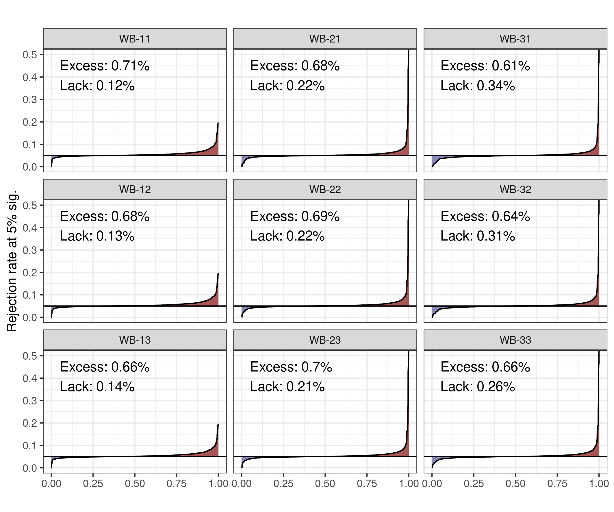
Figure C1: Rejection rates for different wild bootstrap specifications

Similar to the findings of MacKinnon et al. (2023) for the cluster-robust wild bootstrap, the asymmetric specifications WB-31 and WB-13, which utilize HC3 exclusively for the adjustment of the original OLS residuals or solely for the computation of standard errors, respectively, tend to exhibit superior performance. However, the performance differences among the various wild bootstrap specifications are relatively minor.

Figure C2 compares the rejection rates of the three bootstrap specifications WB-11, WB-31, and WB-13 with the alternative specifications, focusing on the 1371  test situations for which bootstrap standard errors are evaluated. While the wild bootstrap specifications exhibit lower average excess in rejection rates than the HC1 and HC2 specificatons, their average excess remains higher than that of HC2-BM, HC3, HC1-PL, and HC2-PL.

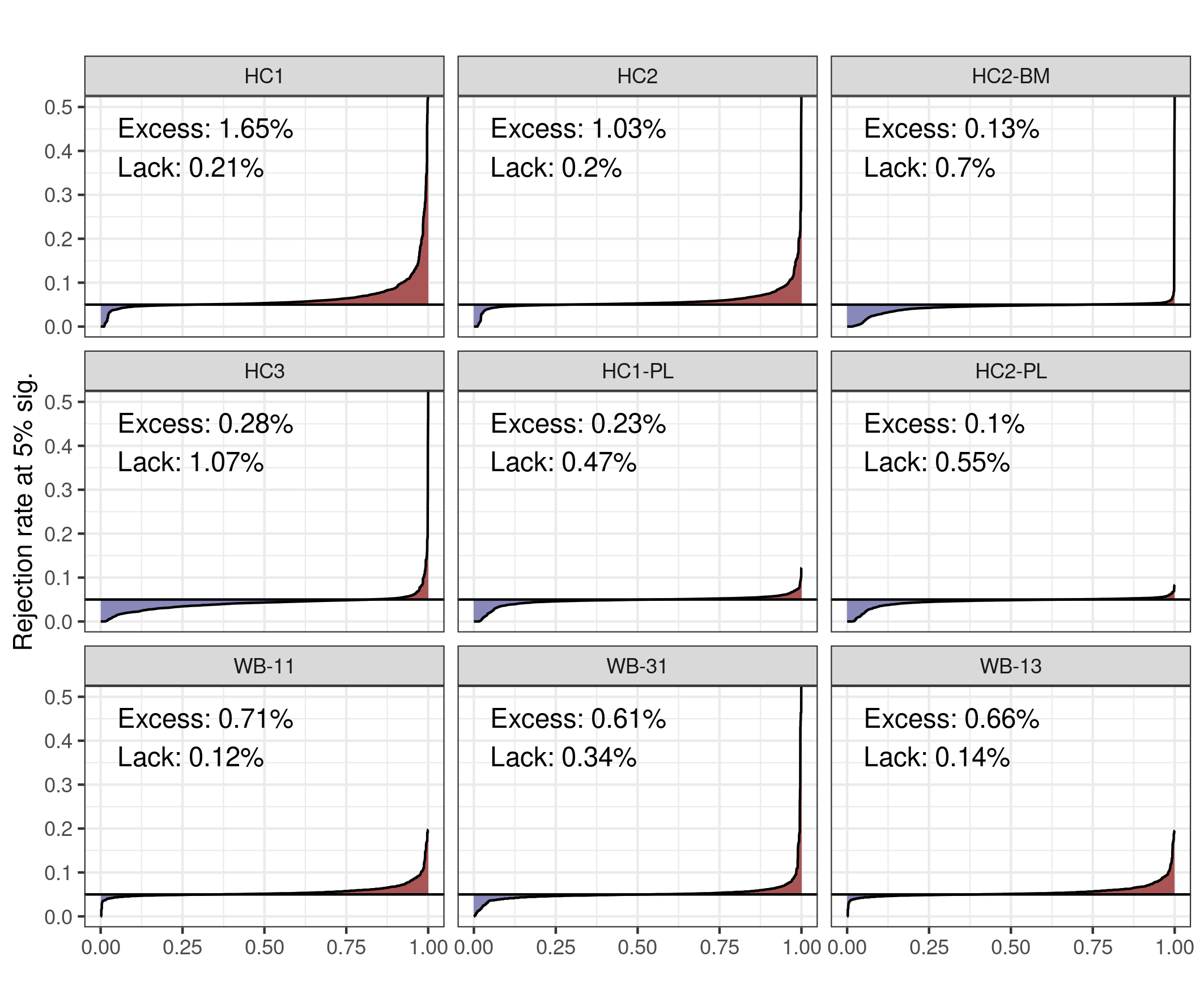
Figure C2: Comparing rejection rates for wild bootstrap specifications with non-bootstrap specifications

Appendix D: Motivating HC1-PL and HC2-PL by a Satterthwaite Approximation

This appendix provides an alternative motivation of the proposed degree of freedom adjustment of HC1-PL and HC2-PL based on $\tilde{n}_{k}$. We start with the regression model

$$y=X\beta+\varepsilon$$

with independently, normally distributed, heteroskedastic errors

$$\varepsilon_{i}\sim N(0,\sigma_{i}^{2}).$$

Let $\hat{V}_{k}^{\tau}$ be a variance estimator of the coefficient $\hat{\beta}_{k}$ and consider the t-test for the null hypothesis $\beta_{k}=0$ with test statistic

$$t_{k}=\frac{\hat{\beta_{k}}}{\sqrt{\hat{V}_{k}^{\tau}}}$$

Following the approximation proposed by Satterthwaite (1946) $t_{k}$ follows approximately a t-distribution with $v_{k}$ degrees of freedom satisfying (see e.g. Christensen, 2018 for a derivation):

$$\nu{}_{k}^{\tau}=\frac{2\text{Var}(\hat{\beta}_{k})^{2}}{\text{Var}\left(\hat{V}_{k}^{\tau}\right)}$$ (7)

We now show that the the partial-leverage adjusted sample size $\tilde{n}_{k}$ approximates $\nu{}_{k}^{HC0}$. Ding (2021) confirms that heteroskedasticity-robust HC0 variances can be directly computed from the FWL representation of the regression:

$$\tilde{y}_{k}=\beta_{k}\tilde{x}_{k}+\tilde{\varepsilon}_{k},$$

yielding

$$\hat{V}_{k}^{HC0}=\frac{\sum_{i=1}^{n}\hat{\varepsilon}_{i}^{2}\tilde{x}_{k,i}^{2}}{\left(\sum_{i=1}^{n}\tilde{x}_{k,i}^{2}\right)^{2}}.$$

Recall that the original OLS residuals $\hat{\varepsilon}_{i}$ are the same as in the FWL specification. We first aim to find

$$\text{Var}(\hat{V}_{k}^{HC0})=\text{Var}\left(\frac{\sum_{i=1}^{n}\hat{\varepsilon}_{i}^{2}\tilde{x}_{i}^{2}}{\left(\sum_{i=1}^{n}\tilde{x}_{i}^{2}\right)^{2}}\right)=\frac{\text{Var}(\sum_{i=1}^{n}\hat{\varepsilon}_{i}^{2}\tilde{x}_{i}^{2})}{\left(\sum_{i=1}^{n}\tilde{x}_{i}^{2}\right)^{4}}.$$

We approximate the variance of the sum in the numerator by the sum of variances

$$\text{Var}(\sum_{i=1}^{n}\hat{\varepsilon}_{i}^{2}\tilde{x}_{k,i}^{2})\approx\sum_{i=1}^{n}\text{Var}\left(\hat{\varepsilon}_{i}^{2}\tilde{x}_{k,i}^{2}\right)=\sum_{i=1}^{n}\tilde{x}_{k,i}^{4}\text{Var}\left(\hat{\varepsilon}_{i}^{2}\right).$$

This approximation is not exact, as OLS residuals $\hat{\varepsilon}_{i}$ can be correlated with each other, even though the original error terms $\varepsilon_{i}$ are assumed to be independently distributed. However, under the common assumptions for a consistent OLS estimator, particularly strong exogeneity, $E(\varepsilon\mid X)=0$, the OLS estimator $\hat{\beta}$ converges to $\beta$ as the sample size increases, and the correlation of the OLS residuals $\hat{\varepsilon}_{i}$ and their squares $\hat{\varepsilon}_{i}^{2}$ vanishes.

We now further approximate

$$\text{Var}\left(\hat{\varepsilon}_{i}^{2}\right)\approx\text{Var}\left(\varepsilon_{i}^{2}\right)=\mathbb{E}\left[\varepsilon_{i}^{4}\right]-\left(\mathbb{E}\left[\varepsilon_{i}{}^{2}\right]\right)^{2}=3\sigma_{i}^{4}-\sigma_{i}^{4}=2\sigma_{i}^{4}$$

where we use the fact that normally distributed errors $\varepsilon_{i}$ satisfy

$$\mathbb{E}\left[\varepsilon_{i}^{4}\right]=3\sigma_{i}^{4}$$

In a further simplification, we follow Bell and McCaffrey (2002) and evaluate the resulting expressions for the case of homoskedasticity

$$\sigma_{i}=\sigma\ \forall i=1,...,N$$

We then find

$$\text{Var}(\hat{V}_{k}^{HC0})\approx 2\sigma^{4}\frac{\sum_{i=1}^{n}\tilde{x}_{k,i}^{4}}{\left(\sum_{i=1}^{n}\tilde{x}_{k,i}^{2}\right)^{4}}.$$

The numerator of (7) under homoskedasticity is given by

$$2\text{Var}(\hat{\beta}_{k})^{2}=2\sigma^{4}\frac{\left(\sum_{i=1}^{n}\tilde{x}_{k,i}^{2}\right)^{2}}{\left(\sum_{i=1}^{n}\tilde{x}_{k,i}^{2}\right)^{4}}.$$

We thus can approximate the degrees of freedom as

$$\nu_{k}^{HC0}=\frac{2\text{Var}(\hat{\beta}_{k})^{2}}{\text{Var}\left(\hat{V}_{k}^{HC0}\right)}\approx\frac{\left(\sum_{i=1}^{n}\tilde{x}_{k,i}^{2}\right)^{2}}{\sum_{i=1}^{n}\tilde{x}_{k,i}^{4}}=\tilde{n}_{k}$$

It is clear that this derivation involves several approximations, and we would not propose our degree of freedom adjustment solely based on this result, especially since we suggest using $\tilde{n}_{k}-1$ degrees of freedom instead of $\tilde{n}_{k}$. Nonetheless, the derivation provides additional insight into why our proposal may be a reasonable choice.

The main differences between this derivation and that of Bell and McCaffrey (2002) are as follows: First, their computation of degrees of freedom is based on an HC2 correction. Second, they do not use the Frisch-Waugh-Lovell (FWL) representation as the starting point for their approximation.