Recursive Gaussian Process State Space Model

Abstract

Learning dynamical models from data is not only fundamental but also holds great promise for advancing principle discovery, time-series prediction, and controller design. Among various approaches, Gaussian Process State-Space Models (GPSSMs) have recently gained significant attention due to their combination of flexibility and interpretability. However, for online learning, the field lacks an efficient method suitable for scenarios where prior information regarding data distribution and model function is limited. To address this issue, this paper proposes a recursive GPSSM method with adaptive capabilities for both operating domains and Gaussian process (GP) hyperparameters. Specifically, we first utilize first-order linearization to derive a Bayesian update equation for the joint distribution between the system state and the GP model, enabling closed-form and domain-independent learning. Second, an online selection algorithm for inducing points is developed based on informative criteria to achieve lightweight learning. Third, to support online hyperparameter optimization, we recover historical measurement information from the current filtering distribution. Comprehensive evaluations on both synthetic and real-world datasets demonstrate the superior accuracy, computational efficiency, and adaptability of our method compared to state-of-the-art online GPSSM techniques.

I Introduction

State-space models (SSMs), also known as hidden Markov models (HMMs), describe the evolution and observation processes of latent states through a state transition model and a measurement model. By summarizing historical information into the latent state, SSMs provide a concise representation of system dynamics and are widely applied in fields such as finance [1], neuroscience [2], target tracking [3], and control systems [4]. Nevertheless, due to the complexity of real-world systems, establishing precise SSMs based on first principles is challenging. To achieve sufficiently accurate system models, extensive research has focused on data-driven SSM modeling [5, 6, 7].

In the past decade, a novel SSM learning method based on the Gaussian process (GP), a nonparametric modeling technique, has been explored [8, 7]. This approach models the transition and measurement functions of SSMs as GPs, and is therefore referred to as Gaussian process state-space models (GPSSMs) [7]. By employing GPs, GPSSMs offer flexible learning for the transition and measurement functions and provide prediction uncertainty, which is crucial for safety-critical applications [9]. To date, various GPSSM methods have been developed, including sample-based methods [10, 11, 12] and variational inference (VI)-based methods [13, 14, 15, 16, 17, 18]. Among these, most studies focus solely on offline scenarios. However, in engineering practice, many systems experience non-stationary changes (e.g., drone propeller performance varies with battery levels), and there is the possibility of operating in out-of-distribution settings. This underscores the urgent need for an online learning method for GPSSMs, which is the focus of this paper.

Facilitating online learning for GPSSMs presents significant challenges. Beyond the usual constraints associated with online learning—such as minimizing memory usage, reducing computational complexity, and preventing catastrophic forgetting—GPSSMs pose additional, unique difficulties. These challenges are detailed as follows. (1) Nonlinearity complicates inference. In GPSSMs, the system state is included in the input to the GP model, introducing inherent nonlinearity. This nonlinearity is intractable, which prevents exact inference through analytic methods. (2) Nonparametric nature of GP. For standard Gaussian process regression (GPR), the training complexity scales cubically with the number of samples [19]. In an online context, as new data arrives continuously, the computational cost of GPs increases rapidly, rendering inference intractable. (3) Coupling between the system state and the system model. Since the state is implicitly measured, learning the system model requires inferring the system state. However, state inference depends on the system model itself. As a result, there is a coupling between the state and the model, which increases the complexity of inference. Theoretically, since both are uncertain, they should be treated as latent variables and inferred simultaneously. (4) Hyperparameter online optimization. GPSSMs involve several hyperparameters, such as GP kernel parameters, which impact the learning accuracy. In online settings, hyperparameter optimization presents two main challenges. First, due to memory efficiency considerations, historical measurements are not retained in online scenarios, depriving hyperparameter optimization of explicit information sources. Secondly, since the GP prior depends on kernel hyperparameters, tuning these parameters requires corresponding adjustments to the posterior distribution. Hence, the online GPSSM problem is quite challenging, and as a result, relevant research remains limited.

Theoretically, implementing online GPSSMs involves Bayesian inference. Therefore, existing methods primarily rely on Bayesian filtering or online variational inference techniques, which can be classified into three categories:

1. Augmented Kalman Filter (AKF)-based method [3, 20, 21]. This approach can jointly infer the system state and the GP model online, and its implementation involves two steps: first, parameterizing the GP with a limited number of parameters using inducing-point approximation [3, 20], or spectral approximation [21]; and second, augmenting the GP model parameters into the state space and inferring the augmented state using the extended Kalman filter (EKF). Through the AKF-based framework, this method achieves recursive learning and offers advantages in learning speed and stability. However, there is a key limitation: the parameterization of the GP requires prior knowledge of the operating domain, specifically the location of inducing points or the range of basis functions in spectral approximation [21]. This drawback limits the approach’s ability to adapt to the flexible distribution of online data. In addition, there is no feasible method for hyperparameter optimization for this approach.

2. Particle Filter (PF)-based method [22, 23, 24]. This approach is similar to the first, with the key difference being the use of the particle filter (PF) for the inference process. Since PF is inefficient at handling high-dimensional states, GP parameters are not augmented into the state space. Instead, each particle is assigned a GP, which is recursively learned using the particle state. This method can theoretically achieve precise inference for arbitrary observational distributions, provided the number of particles is sufficient. However, despite the inherent issues with PF, such as high computational cost and particle degeneracy [25], it also requires prior knowledge of the operating domain.

3. Stochastic Variational Inference (SVI)-based method [11, 18, 26]. This approach extends the offline variational inference method of GPSSMs by utilizing stochastic optimization techniques. It aims to retain many of the benefits of offline GPSSMs, such as a flexible operating domain and hyperparameter optimization capabilities. However, stochastic optimization assumes that the data subsampling process is uniformly random, which is not the case in most online situations. As a result, the learning process is driven by instantaneous data, leading to slow learning and catastrophic forgetting.

In summary, the existing methods either lack the ability to tune the operating domains and hyperparameters, or they face issues with learning speed and convergence.

To overcome the aforementioned shortcomings, a recursive learning algorithm for GPSSMs is proposed in this paper, capable of online adaptation to the operating domain and GP hyperparameters. The main contributions can be summarized as follows: Firstly, to implement a domain-independent recursive learning algorithm for GPSSMs, a novel Bayesian update equation is derived without pre-parameterizing the GP. In the derivation process, only mild linearization approximations are applied to achieve a closed-form solution, offering advantages in learning speed and stability. Through continuously expanding the inducing-point set, this method can accommodate real-time data distributions. Secondly, to address the computational cost issue caused by the increasing number of inducing points, an selection algorithm is developed with both addition and removal operations. To minimize accuracy loss, an optimal discarding equation and selection metric for inducing points are derived based on informative criteria. Thirdly, to alleviate the burden of offline hyperparameter tuning, an online GP hyperparameter optimization method is proposed. In this method, an approximate observation likelihood model is extracted from the obtained posterior distribution. Utilizing this likelihood model as the information source, the GP hyperparameters are optimized, and the posterior distribution can be adjusted as the hyperparameters change. Finally, we validate the effectiveness of the proposed method through two synthetic simulations and a real-world dataset. The experimental results demonstrate the superior performance of the proposed method in terms of learning accuracy, computational efficiency, and adaptive capacity for operating domains and hyperparameters.

II Problem Formulation

In this section, we first briefly provide the background of Gaussian processes (GPs) and then give a definition of Gaussian process state-space models (GPSSMs) and the associated online learning problem.

II-A Gaussian Processes

Mathematically, GP is a probability distribution over function space, which can be employed for regression task. For learning a single-input function $f(\cdot)$, one can first place a GP prior on it:

$$f(\textbf{x})\sim\mathcal{GP}\left(m_{0}(\textbf{x}),\boldsymbol{K}_{0}(\textbf{x},\textbf{x}^{\prime};\boldsymbol{\theta})\right)$$ (1)

where $m_{0}(\cdot)$ denotes the prior mean function and $K_{0}(\cdot,\cdot)$ represents the prior covariance function (also known as kennel function), and $\boldsymbol{\theta}$ denotes the kernel hyperparameters. As a common setting, we assume zero-mean GP prior, namely, $m_{0}(\cdot)\equiv 0$. Then, given function values $\boldsymbol{f}_{\mathbf{X}}$ at input locations $\mathbf{X}$, the posterior distribution for test function values $\boldsymbol{f}_{*}$ is [19]:

$$p(\boldsymbol{f}_{*}|\boldsymbol{f}_{\mathbf{X}})=\mathcal{N}(\boldsymbol{K}_{*\textbf{X}}\boldsymbol{K}_{\textbf{XX}}^{-1}\boldsymbol{f}_{\mathbf{X}},\boldsymbol{K}_{**}-\boldsymbol{K}_{*\textbf{X}}\boldsymbol{K}_{\textbf{XX}}^{-1}\boldsymbol{K}_{\textbf{X}*})$$ (2)

Here, we use shorthand notation for the kernel matrix, e.g., $\boldsymbol{K}_{**}$ denotes the auto-covariance of $\boldsymbol{f}_{*}$, and $\boldsymbol{K}_{*\textbf{X}}$ the cross-covariance between $\boldsymbol{f}_{*}$ and $\boldsymbol{f}_{\textbf{X}}$. This notation is used throughout. Indeed, GPs can be utilized to learn multi-output functions by employing an associated kernel. However, for simplicity, the elaboration of the proposed method is based on the single-output GP, and its extension to the multi-output case is straightforward and will be demonstrated in the experiments.

II-B Online Gaussain Processs State Space Models

In this paper, we consider the following discrete-time state-space model (SSM):

$$\boldsymbol{x}_{t+1} =\boldsymbol{F}(\boldsymbol{x}_{t},f(\boldsymbol{x}_{t}))+\boldsymbol{\omega}_{f}, \boldsymbol{\omega}_{f}\sim\mathcal{N}(\boldsymbol{0},\boldsymbol{\Sigma}_{f})$$ (3)

$$\boldsymbol{y}_{t} =\boldsymbol{g}(\boldsymbol{x}_{t})+\boldsymbol{\omega}_{g}, \boldsymbol{\omega}_{g}\sim\mathcal{N}(\boldsymbol{0},\boldsymbol{\Sigma}_{g})$$

where the vector $\boldsymbol{x}\in\mathbb{R}^{n_{x}}$ and $\boldsymbol{y}\in\mathbb{R}^{n_{y}}$ respectively denote the system state and measurement. The vectors $\boldsymbol{\omega}_{f}$ and $\boldsymbol{\omega}_{g}$ represent the process and measurement noise, with covariances $\boldsymbol{\Sigma}_{f}$ and $\boldsymbol{\Sigma}_{g}$, respectively. Additionally, the function $\boldsymbol{F}:\mathbb{R}^{n_{x}}\to\mathbb{R}^{n_{x}}$ denotes a known function structure for the transition model , which contains an unknown component, represented as the function $f:\mathbb{R}^{n_{x}}\to\mathbb{R}$. To ensure identifiability, the measurement model $\boldsymbol{g}:\mathbb{R}^{n_{x}}\to\mathbb{R}^{n_{y}}$ is assumed to be known.

To learn the unknown SSMs, GPSSMs place GP priors on the unknown function $f(\cdot)$, resulting in the following model [7]:

$$\boldsymbol{x}_{0}\sim p(\boldsymbol{x}_{0})$$ (4a)

$$f(\cdot)\sim\mathcal{GP}(m_{0}(\cdot),\boldsymbol{K}_{0}(\cdot,\cdot);\boldsymbol{\theta})$$ (4b)

$$\boldsymbol{x}_{t+1}|\boldsymbol{x}_{t},\boldsymbol{f}\sim\mathcal{N}\left(\boldsymbol{x}_{t}\,\big{|}\,\boldsymbol{F}(\boldsymbol{x}_{t},f(\boldsymbol{x}_{t})),\,\boldsymbol{\Sigma}_{f}\right)$$ (4c)

$$\boldsymbol{y}_{t}|\boldsymbol{x}_{t}\sim\mathcal{N}\left(\boldsymbol{y}_{t}\,\big{|}\,\boldsymbol{g}(\boldsymbol{x}_{t}),\,\boldsymbol{\Sigma}_{g}\right)$$ (4d)

where $p(\boldsymbol{x}_{0})$ denotes a prior Gaussian distribution for the initial state $\boldsymbol{x}_{0}$, and note that we use the notation $\boldsymbol{f}$ in (4c) to denote any collection of function values of interest, which includes $f(\boldsymbol{x}_{t})$. For conciseness, we omit the system input from the transition and measurement models, which can be easily incorporated by augmenting it into the input of these models and the GP.

In the online setting, measurements $\boldsymbol{y}$ arrive sequentially, and we assume that historical measurements are not retained for computational and storage reasons. Given this streaming data setting, the inference task of online GPSSMs is to sequentially approximate the filtering distribution $p(\boldsymbol{x}_{t},\boldsymbol{f}|\boldsymbol{y}_{1:t})$, using the previous result $p(\boldsymbol{x}_{t-1},\boldsymbol{f}|\boldsymbol{y}_{1:t-1})$ and the current measurement $\boldsymbol{y}_{t}$. As illustrated in the introduction, several challenges exist in this task, including the nonlinearity and coupling involved, as well as the nonparametric nature of GPs and the hyperparameter optimization problem. To address these difficulties, a novel online GPSSM approach will be developed in the next two sections, with the ability to adapt to both operating domains and hyperparameters.

III Bayesian Update Equation for Online GPSSMs

This section derives a Bayesian update equation for online GPSSMs with minimal approximations to achieve recursive learning in an arbitrarily operating domain.

III-A Two-Step Inference

The online inference of GPSSMs is essentially a filtering problem; therefore, most methods are based on filtering techniques, such as the extended Kalman filter (EKF) and particle filter (PF). Considering that the PF will exacerbate the computational cost issues due to GP and its particle degradation problem, we choose the EKF in this paper. The widely adopted EKF is a two-step version, which is more numerically stable [27] and can handle irregular measurements. In each update, the EKF propagates the state distribution and then corrects it with the current measurement, which are known as the prediction (time update) and correction (measurement update) steps, respectively. In the context of GPSSMs, considering the coupling between the system state and the GP, the distribution to be propagated and corrected is the joint distribution of both. These two operations can be expressed by:

$$p(\boldsymbol{x}_{t+1},\boldsymbol{f}|\boldsymbol{y}_{1:t})=\int p(\boldsymbol{x}_{t+1}|\boldsymbol{x}_{t},\boldsymbol{f})p(\boldsymbol{x}_{t},\boldsymbol{f}|\boldsymbol{y}_{1:t})\mathrm{d}\boldsymbol{x}_{t}$$ (5)

$$p(\boldsymbol{x}_{t+1},\boldsymbol{f}|\boldsymbol{y}_{1:t+1})=\dfrac{p(\boldsymbol{y}_{t+1}|\boldsymbol{x}_{t+1})p(\boldsymbol{x}_{t+1},\boldsymbol{f}|\boldsymbol{y}_{1:t})}{p(\boldsymbol{y}_{t+1}|\boldsymbol{y}_{1:t})}$$ (6)

where $p(\boldsymbol{x}_{t+1}|\boldsymbol{x}_{t},\boldsymbol{f})$ and $p(\boldsymbol{y}_{t+1}|\boldsymbol{x}_{t+1})$ are the transition and measurement densities as defined in (4), $p(\boldsymbol{x}_{t},\boldsymbol{f}|\boldsymbol{y}_{1:t})$ denotes the joint posterior at time $t$, and $p(\boldsymbol{x}_{t+1},\boldsymbol{f}|\boldsymbol{y}_{1:t})$ is the joint prior or predicted distribution at time $t+1$. To evaluate the distribution in equations (5) and (6), the key challenges are the nonparametric nature of the GP and the nonlinearity in the transition and measurement models. Existing methods [20, 3, 21, 22, 23] typically first address the former by pre-parameterizing the GP into a fixed structure and then applying nonlinear filtering to handle the latter. However, pre-parameterization limits the operating domain, thus reducing the algorithm’s flexibility. To overcome this, we reverse the process: first handling the nonlinearity without any GP approximation, then addressing the nonparametric nature. We achieve the first procedure in the next subsection, resulting in an update equation with a factorized approximate distribution.

III-B Factorized Approximate Distribution

To address the nonlinearity within the transition and measurement model, first-order linearization is applied in this subsection, whose result is the following theorem.

Theorem 1

By approximating the transition and measurement models with first-order linearization, the joint distribution between the state and GP obtained in each prediction and correction step follows the factorized form:

$$q(\boldsymbol{x}_{t},\boldsymbol{f})=p(\boldsymbol{f}|\boldsymbol{u})q(\boldsymbol{x}_{t},\boldsymbol{u})$$ (7)

where $\boldsymbol{u}\triangleq\{u_{i}\}_{i=1}^{n_{u}}$ is a collection of a finite number of inducing points, $p(\boldsymbol{f}|\boldsymbol{u})$ is the exact GP conditional distribution similar to (2), and $q(\boldsymbol{x}_{t},\boldsymbol{u})$ is a Gaussian distribution.

Given Theorem 1, the approximate joint distribution remains Gaussian, which can be evaluated using closed-form update equations. In the following, we will prove Theorem 1 and then derive these equations.

To facilitate the proof, we first introduce some notation regarding the approximate distributions $q(\boldsymbol{x}_{t},\boldsymbol{u})$ and $q(\boldsymbol{x}_{t},\boldsymbol{f})$. Specifically, these two distributions are expressed as:

$$q(\boldsymbol{x}_{t},\boldsymbol{u}) =\mathcal{N}\left(\begin{bmatrix}\boldsymbol{x}_{t}\\ \boldsymbol{u}\\ \end{bmatrix}\Bigg{|}\begin{bmatrix}\boldsymbol{\mu}_{t}\\ \boldsymbol{m}_{u}\\ \end{bmatrix},\begin{bmatrix}\boldsymbol{P}_{t}&\boldsymbol{V}_{xu}\\ \boldsymbol{V}_{xu}^{T}&\boldsymbol{S}_{uu}\\ \end{bmatrix}\right)$$ (8)

$$q(\boldsymbol{x}_{t},\boldsymbol{f}) =\mathcal{N}\left(\begin{bmatrix}\boldsymbol{x}_{t}\\ \boldsymbol{f}\\ \end{bmatrix}\Bigg{|}\begin{bmatrix}\boldsymbol{\mu}_{t}\\ \boldsymbol{m}_{f}\\ \end{bmatrix},\begin{bmatrix}\boldsymbol{P}_{t}&\boldsymbol{V}_{xf}\\ \boldsymbol{V}_{xf}^{T}&\boldsymbol{S}_{ff}\\ \end{bmatrix}\right)$$

In this expression, the moments of the joint distribution are distinguished based on the state $\boldsymbol{x}_{t}$ and inducing points $\boldsymbol{u}$ or function values $\boldsymbol{f}$. For $q_{t}(\boldsymbol{x}_{t},\boldsymbol{u})$, the vectors $\boldsymbol{\mu}_{t}$ and $\boldsymbol{m}_{u}$ represent the means of the state $\boldsymbol{x}_{t}$ and the inducing points $\boldsymbol{u}$, respectively. $\boldsymbol{P}_{t}$ denotes the autocovariance of $\boldsymbol{x}_{t}$, while $\boldsymbol{V}_{xu}$ represents the cross-covariance between $\boldsymbol{x}_{t}$ and $\boldsymbol{u}$, and $\boldsymbol{S}_{uu}$ signifies the autocovariance of $\boldsymbol{u}$. For the moments of $q_{t}(\boldsymbol{x}_{t},\boldsymbol{f})$, its notation follow the same logic, and the values are fully specified by the moments of $q(\boldsymbol{x}_{t},\boldsymbol{u})$, specifically:

$$\boldsymbol{m}_{f}=\boldsymbol{k}_{fu}\boldsymbol{m}_{u}$$ (9)

$$\boldsymbol{V}_{xf}=\boldsymbol{V}_{xu}\boldsymbol{k}_{fu}^{T}$$

$$\boldsymbol{S}_{ff}=\boldsymbol{K}_{ff}+\boldsymbol{k}_{fu}\left(\boldsymbol{S}_{uu}-\boldsymbol{K}_{uu}\right)\boldsymbol{k}_{fu}^{T}$$

where $\boldsymbol{k}_{fu}=\boldsymbol{K}_{fu}\boldsymbol{K}_{uu}^{-1}$. This equation can be easily derived by using (7) and the conditional distribution $p(\boldsymbol{f}|\boldsymbol{u})$.

By means of the above notation, we will illustrate the proof of Theorem 1, which is based on mathematical induction. First, it can be demonstrated that at time $0$, the joint distribution naturally satisfies the factorized form (7):

$$p(\boldsymbol{x}_{0},\boldsymbol{f}) =p(\boldsymbol{f})p(\boldsymbol{x}_{0})$$ (10)

$$=p(\boldsymbol{f}|\boldsymbol{u})p(\boldsymbol{u})p(\boldsymbol{x}_{0})$$

$$=p(\boldsymbol{f}|\boldsymbol{u})q(\boldsymbol{x}_{0},\boldsymbol{u})$$

where $p(\boldsymbol{f})$ denotes the GP prior over function values $\boldsymbol{f}$ and $\boldsymbol{u}$ can be any collection of function values or an empty set. Therefore, the next step is to prove that the approximate updates of the prediction and correction steps can preserve the factorized form.

For the prediction step, to address the nonlinearity in the transition model (4c), we employ first-order linearization as in the EKF, specifically linearizing the transition model as follows:

$$p(\boldsymbol{x}_{t+1}|\boldsymbol{x}_{t},\boldsymbol{f})$$ (11)

$$\approx\mathcal{N}\Big{(}\boldsymbol{x}_{t+1}\Big{|}\boldsymbol{F}_{t}+\boldsymbol{A}_{x}(\boldsymbol{x}_{t}-\boldsymbol{\mu}_{t})+\boldsymbol{A}_{f}(f_{t}-m_{f_{t}}),\boldsymbol{\Sigma}_{f}\Big{)}$$

$$=\hat{p}(\boldsymbol{x}_{t+1}|\boldsymbol{x}_{t},f_{t}).$$

where we use the notation for moments in (8) and the shorthand notation $f_{t}=f(\boldsymbol{\mu}_{t})$, $\boldsymbol{F}_{t}=\boldsymbol{F}(\boldsymbol{\mu}_{t},m_{f_{t}})$. Additionally, the two Jacobian matrices are $\boldsymbol{A}_{x}=\partial\boldsymbol{F}(\boldsymbol{x},m_{f(\boldsymbol{x})})/\partial\boldsymbol{x}|_{\boldsymbol{\mu}_{t}}$ and $\boldsymbol{A}_{f}=\partial\boldsymbol{F}(\boldsymbol{\mu}_{t},f)/\partial f|_{m_{f_{t}}}$. Note that, we use the hat notation $\hat{p}(\boldsymbol{x}_{t+1}|\boldsymbol{x}_{t},f_{t})$ in (11) to denote the linearized model. As shown in (11), this linearized transition model depends solely on the function value $f_{t}$. Therefore, if we incorporate $f_{t}$ into the inducing-point set, i.e., $\bar{\boldsymbol{u}}=[\boldsymbol{u}^{T},f_{t}^{T}]^{T}$, the prediction result in (5) by using the linearized model (11) retains the factorized form (7):

$$q^{-}(\boldsymbol{x}_{t+1},\boldsymbol{f}) =\int q(\boldsymbol{x}_{t},\boldsymbol{f})\hat{p}(\boldsymbol{x}_{t+1}|\boldsymbol{x}_{t},f_{t})\mathrm{d}x_{t}$$ (12)

$$=p(\boldsymbol{f}|\bar{\boldsymbol{u}})\int q(\boldsymbol{x}_{t},\bar{\boldsymbol{u}})\hat{p}(\boldsymbol{x}_{t+1}|\boldsymbol{x}_{t},f_{t})\mathrm{d}\boldsymbol{x}_{t}$$

$$=p(\boldsymbol{f}|\bar{\boldsymbol{u}})q^{-}(\boldsymbol{x}_{t+1},\bar{\boldsymbol{u}})$$

where we use the superscript ”-” to denote predicted distributions, and $q^{-}(\boldsymbol{x}_{t+1},\bar{\boldsymbol{u}})=\int q(\boldsymbol{x}_{t},\bar{\boldsymbol{u}})\hat{p}(\boldsymbol{x}_{t+1}|\boldsymbol{x}_{t},f_{t})\mathrm{d}\boldsymbol{x}_{t}$. It can be observed that the factorized form is preserved at the cost of augmenting the inducing-point set, an inevitable consequence of the non-parametric nature of the GP. This increase in the number of inducing points leads to a rapid rise in computational burden, rendering inference intractable, which will be addressed in Section IV-A.

For the correction step, the derivation is similar. To handle the nonlinearity in the measurement model (4d), the first-order linearization is used again:

$$p(\boldsymbol{y}_{t+1}|\boldsymbol{x}_{t+1})$$ (13)

$$\approx\mathcal{N}\left(\boldsymbol{y}_{t+1}\bigg{|}\boldsymbol{g}(\boldsymbol{\mu}_{t+1}^{-})+\boldsymbol{C}(\boldsymbol{x}_{t+1}-\boldsymbol{\mu}_{t+1}^{-}),\boldsymbol{\Sigma}_{g}\right)$$

$$=\hat{p}(\boldsymbol{y}_{t+1}|\boldsymbol{x}_{t+1})$$

where $\boldsymbol{\mu}_{t+1}^{-}$ denotes the predicted mean of state $\boldsymbol{x}_{t+1}$ and the measurement Jacobian is $\boldsymbol{C}=\partial\boldsymbol{g}(\boldsymbol{x})/\partial\boldsymbol{x}\big{|}_{\boldsymbol{\mu}_{t+1}^{-}}$. By incorporating this linearized model into the correction step (6), the factorized form can be retained as follows:

$$q(\boldsymbol{x}_{t+1},\boldsymbol{f}) \propto q^{-}(\boldsymbol{x}_{t+1},\boldsymbol{f})\hat{p}(\boldsymbol{y}_{t+1}|\boldsymbol{x}_{t+1})$$ (14)

$$=p(\boldsymbol{f}|\bar{\boldsymbol{u}})q^{-}(\boldsymbol{x}_{t+1},\bar{\boldsymbol{u}})\hat{p}(\boldsymbol{y}_{t+1}|\boldsymbol{x}_{t+1})$$

$$\propto p(\boldsymbol{f}|\bar{\boldsymbol{u}})q(\boldsymbol{x}_{t+1},\bar{\boldsymbol{u}})$$

where $q(\boldsymbol{x}_{t+1},\bar{\boldsymbol{u}})\propto q^{-}(\boldsymbol{x}_{t+1},\bar{\boldsymbol{u}})\hat{p}(\boldsymbol{y}_{t+1}|\boldsymbol{x}_{t+1})$.

Thus far, we have proven Theorem 1, where only first-order linearization is used, and the inducing-point set is continually expanded to match the data distribution. For the linearization treatment involved, it provides a high-accuracy approximation when the nonlinearity is weak and the variance of the joint distribution is small. In the derivation, we also obtain the approximate prediction equation (12) and correction equation (14) for the joint distribution $q(\boldsymbol{x}_{t},\boldsymbol{f})$, which can be used to derive practical update equations for it. It is evident that the joint distribution $q(\boldsymbol{x}_{t},\boldsymbol{u})$ contains the essential information of $q(\boldsymbol{x}_{t},\boldsymbol{f})$ and thus is the only component that requires updating. The moment update equations for it are derived in the next subsection.

III-C Moment Update Equation

For simplicity in the moment update equation, we define the union of the system state and inducing points as an augmented state, i.e., $\boldsymbol{X}_{t}=[\boldsymbol{x}_{t}^{T},\boldsymbol{u}^{T}]^{T}$. Consequently, the approximate distribution $q(\boldsymbol{x}_{t},\boldsymbol{u})$ can be expressed as $q(\boldsymbol{X}_{t})$, with its mean and covariance denoted as $\boldsymbol{\xi}_{t}$ and $\boldsymbol{\Sigma}_{t}$, respectively. Based on this definition, the moment update equation becomes a recursive equation for $\boldsymbol{\xi}_{t}$ and $\boldsymbol{\Sigma}_{t}$.

For the prediction step, given the update equation (12), we should first add the point $f_{t}$ into the inducing point set $\boldsymbol{u}$, thus obtaining the new set $\bar{\boldsymbol{u}}$. Therefore, we define the new augmented state $\bar{\boldsymbol{X}}_{t}=[\boldsymbol{x}_{t}^{T},\bar{\boldsymbol{u}}^{T}]^{T}$, similar to $\boldsymbol{X}_{t}$. Correspondingly, we have the approximate distribution $q(\bar{\boldsymbol{X}}_{t})$ with mean $\bar{\boldsymbol{\xi}}_{t}$ and covariance $\bar{\boldsymbol{\Sigma}}_{t}$, which can be evaluated using (8) and (9) by letting $\boldsymbol{f}=\bar{\boldsymbol{u}}$. Then, by applying the update equation (12), the moment update equation for the prediction step can be easily derived, with a result similar to that of the EKF.

$$\bar{\boldsymbol{\xi}}_{t+1}^{-}=[\boldsymbol{F}_{t}^{T},\boldsymbol{m}_{\bar{u}}^{T}]^{T}$$ (15)

$$\bar{\boldsymbol{\Sigma}}_{t+1}^{-}=\boldsymbol{\Phi}\bar{\boldsymbol{\Sigma}}_{t}\boldsymbol{\Phi}^{T}+\boldsymbol{\Sigma}_{f,\bar{X}}$$

$$\boldsymbol{\Phi}=\begin{bmatrix}\boldsymbol{A}_{x}&\boldsymbol{0}&\boldsymbol{A}_{f}\\ \boldsymbol{0}&\boldsymbol{I}_{n_{u}}&\boldsymbol{0}\\ \boldsymbol{0}&\boldsymbol{0}&1\\ \end{bmatrix}$$

$$\boldsymbol{\Sigma}_{f,\bar{X}}=\begin{bmatrix}\boldsymbol{\Sigma}_{f}&\boldsymbol{0}\\ \boldsymbol{0}&\boldsymbol{0}\\ \end{bmatrix}$$

where $\bar{\boldsymbol{\xi}}_{t+1}^{-}$ and $\bar{\boldsymbol{\Sigma}}_{t+1}^{-}$ represent the predicted mean and covariance for the augmented state $\bar{\boldsymbol{X}}_{t+1}$, $\boldsymbol{\Phi}$ denotes its transition Jacobian matrix, and $\boldsymbol{\Sigma}_{f,\bar{X}}$ is its process noise covariance.

For the correction step, the moment update equation can be easily obtained using the approximate correction equation in (14), with the result as follows:

$$\boldsymbol{H}=\begin{bmatrix}\boldsymbol{C}&\boldsymbol{0}\\ \end{bmatrix}$$ (16)

$$\boldsymbol{G}=\bar{\boldsymbol{\Sigma}}_{t+1}^{-}\boldsymbol{H}^{T}\left(\boldsymbol{C}\boldsymbol{P}_{t+1}^{-}\boldsymbol{C}^{T}+\boldsymbol{\Sigma}_{g}\right)^{-1}$$

$$\bar{\boldsymbol{\xi}}_{t+1}=\bar{\boldsymbol{\xi}}_{t+1}^{-}+\boldsymbol{G}\left[\boldsymbol{y}_{t+1}-\boldsymbol{g}(\boldsymbol{\mu}_{t+1}^{-})\right]$$

$$\bar{\boldsymbol{\Sigma}}_{t+1}=\bar{\boldsymbol{\Sigma}}_{t+1}^{-}-\boldsymbol{G}\boldsymbol{H}\bar{\boldsymbol{\Sigma}}_{t+1}^{-}$$

where $\boldsymbol{P}_{t+1}^{-}$ denotes the predicted variance of the system state $\boldsymbol{x}_{t+1}$, $\bar{\boldsymbol{\xi}}_{t+1}$ and $\bar{\boldsymbol{\Sigma}}_{t+1}$ represent the posterior mean and covariance for the augmented state $\bar{\boldsymbol{X}}_{t+1}$, $\boldsymbol{H}$ is its measurement Jacobian, and $\boldsymbol{G}$ corresponds to the Kalman gain. Therefore, through the moment update equations (15) and (16), closed-form recursive inference for online GPSSMs can be achieved.

In summary, this section derives a two-step form of the Bayesian update equation for online GPSSMs, where first-order linearization approximations are used to handle the nonlinearity of the transition and measurement models. The derivation shows that, by applying linearization and augmenting the inducing-point set, the joint distribution retains a factorized structure, leading to the moment update equations (15) and (16). These equations enable recursive learning for GPSSMs without the constraint of an operating domain. However, as discussed in Section III-B, the increasing number of inducing points significantly raises the computational burden for moment evaluation, making inference intractable. In the next section, an approximation method will be introduced to address this issue.

IV Adaptation of Inducing points and Hyperparameters

While the recursive learning algorithm for GPSSMs has been developed, two issues remain: the computational burden problem due to the non-parameteric nature of GP, and the hyperparameter online adaptation problem. In Section IV-A, a pseudo-point set adjustment algorithm is introduced to maintain limited computational complexity, and in Section IV-B, an online hyperparameter adaptation method is derived to improve learning accuracy.

IV-A Dynamic Adjusting the Inducing Points Set

As discussed in Section III, the computational complexity of the learning algorithm increases with the addition of inducing points. This challenge is also encountered in the development of kernel-based online regression algorithms, such as Kernel Recursive Least Squares (KRLS) [28] and Sparse Online Gaussian Processes (SOGP) [29, 30]. These two methods are, to some extent, equivalent and control computational cost by limiting the size of the inducing point set within a predefined budget $M$. Specifically, this strategy is achieved through two operations: discarding the least important point when the set exceeds the budget $M$, and adding only sufficiently novel points. To implement the discarding and adding operations, the following two key problems must be addressed: (1) how to remove a point with minimal accuracy loss, and (2) how to evaluate the importance or novelty of a point. In the following, we will address these two problems in the context of GPSSMs and develop an adjustment method for the inducing point set, thereby overcoming the computational burden issue. For convenience, let $u_{d}$ denote the inducing point to be discarded, with index $i_{d}$ in the point set, and let $\boldsymbol{u}_{l}$ represent the remaining inducing points.

For the first problem, we define that the new joint distribution, after discarding point $u_{d}$, still retains the factorized form (7), namely, $\hat{q}(\boldsymbol{x},\boldsymbol{f})=p(\boldsymbol{f}|\boldsymbol{u})\hat{q}(\boldsymbol{x},\boldsymbol{u}_{l})$, where $\hat{q}(\boldsymbol{x},\boldsymbol{u}_{l})$ is Gaussian. Then, to ensure minimal accuracy loss, we can seek the optimal solution within the distribution family of $\hat{q}(\boldsymbol{x},\boldsymbol{f})$, such that the distance between it and the original joint distribution $q(\boldsymbol{x},\boldsymbol{f})=p(\boldsymbol{f}|\boldsymbol{u})q(\boldsymbol{x},\boldsymbol{u})$ is minimized. Since $\hat{q}(\boldsymbol{x},\boldsymbol{u}_{l})$ controls the approximate distribution $\hat{q}(\boldsymbol{x},\boldsymbol{f})$, it is sufficient to find its optimal distribution. Here, we use the inclusive KL divergence as a distance metric, namely $\mathrm{KL}[q\|\hat{q}]=\int q\log\left(q/\hat{q}\right)$, which results in a simple optimal distribution:

$$\hat{q}^{*}(\boldsymbol{x},\boldsymbol{u}_{l}) =\arg\min\limits_{\hat{q}(\boldsymbol{x},\boldsymbol{u}_{l})}\mathrm{KL}\left[q(\boldsymbol{x},\boldsymbol{f})\|\hat{q}(\boldsymbol{x},\boldsymbol{f})\right]$$ (17)

$$=\arg\min\limits_{\hat{q}(\boldsymbol{x},\boldsymbol{u}_{l})}\mathrm{KL}\left[p(\boldsymbol{f}|\boldsymbol{u})q(\boldsymbol{x},\boldsymbol{u})\|p(\boldsymbol{f}|\boldsymbol{u}_{l})\hat{q}(\boldsymbol{x},\boldsymbol{u}_{l})\right]$$

$$=\arg\min\limits_{\hat{q}(\boldsymbol{x},\boldsymbol{u}_{l})}\mathrm{KL}\left[q(\boldsymbol{x},\boldsymbol{u})\|p(u_{d}|\boldsymbol{u}_{l})\hat{q}(\boldsymbol{x},\boldsymbol{u}_{l})\right]$$

$$=\int q(\boldsymbol{x},\boldsymbol{u})\,\mathrm{d}u_{d}$$

It can be observed that the optimal distribution $\hat{q}^{*}(\boldsymbol{x},\boldsymbol{u}_{l})$ only involves marginalizing the discarded inducing point $u_{d}$ from the original distribution. Through (17), optimal deletion for a given inducing point can be achieved.

Furthermore, for the second problem, the importance or novelty of a point can be assessed by the accuracy loss incurred from optimally discarding it. Specifically, this can be done by calculating the KL divergence in (17) with $\hat{q}(\boldsymbol{x},\boldsymbol{u}_{l})=\hat{q}^{*}(\boldsymbol{x},\boldsymbol{u}_{l})$:

$$D^{*} =\mathrm{KL}\left[q(\boldsymbol{x},\boldsymbol{u})\|p(u_{d}|\boldsymbol{u}_{l})\hat{q}^{*}(\boldsymbol{x},\boldsymbol{u}_{l})\right]$$ (18)

$$=D_{1}-D_{2}-D_{3}$$

$$D_{1} =\int q(\boldsymbol{x},\boldsymbol{u})\log q(\boldsymbol{x},\boldsymbol{u})\,\mathrm{d}\boldsymbol{x}\,\mathrm{d}\boldsymbol{u}$$

$$D_{2} =\int q(\boldsymbol{u})\log p(u_{d}|\boldsymbol{u}_{l})\,\mathrm{d}\boldsymbol{u}$$

$$D_{3} =\int\hat{q}^{*}(\boldsymbol{x},\boldsymbol{u}_{l})\log\hat{q}^{*}(\boldsymbol{x},\boldsymbol{u}_{l})\,\mathrm{d}\boldsymbol{u}_{l}$$

Through the KL divergence $D^{*}$, the accuracy loss from discarding the inducing point $u_{d}$ can be evaluated. A computable score $s_{d}$ quantifying the accuracy loss can be obtained by dropping the $u_{d}$-irrelevant terms in (18) (the derivation is deferred to Appendix A), namely:

$$s_{d} =\Delta_{1}+\Delta_{2}+\Delta_{3}$$ (19)

$$\Delta_{1} =\boldsymbol{m}_{u}^{T}\boldsymbol{Q}_{du}^{T}\boldsymbol{Q}_{dd}^{-1}\boldsymbol{Q}_{du}\boldsymbol{m}_{u}$$

$$\Delta_{2} =\mathrm{tr}\left(\boldsymbol{Q}_{du}\boldsymbol{S}_{uu}\boldsymbol{Q}_{du}^{T}\boldsymbol{Q}_{dd}^{-1}\right)$$

$$\Delta_{3} =\log|\boldsymbol{\Omega}_{dd}|-\log|\boldsymbol{Q}_{dd}|$$

where we denote the inverse of the joint covariance as $\boldsymbol{\Omega}=\boldsymbol{\Sigma}_{t}^{-1}$, and $\boldsymbol{\Omega}_{dd}$ is the element of the matrix $\boldsymbol{\Omega}$ corresponding to the discarded point $u_{d}$, namely, its $(n_{x}+i_{d})$-th diagonal element. In addition, $\boldsymbol{Q}_{dd}$ and $\boldsymbol{Q}_{du}$ are the $i_{d}$-th diagonal element and the $i_{d}$-th row of the inverse kernel matrix $\boldsymbol{Q}=\boldsymbol{K}_{uu}^{-1}$. Among the terms in (19), $\Delta_{1}$ represents the accuracy loss in the mean of joint distribution $q(\boldsymbol{x}_{t},\boldsymbol{f})$, which matches the result in KRLS [28], while $\Delta_{1}$ and $\Delta_{2}$ correspond to the loss in the covariance. Overall, the score $s_{d}$ quantifies the relative accuracy loss from discarding $u_{d}$, with a smaller score indicating a smaller accuracy loss.

Through (17) and (19), we have addressed the two key challenges. Based on these, we can provide the adjustment rule for the inducing point set, which is divided into discarding and adding operations. For the discarding operation, the rule is as follows: if the size of the inducing point set exceeds the budget $M$, evaluate the score of each point using (19) and remove the one with the lowest score. According to (17), the moments of the new joint distribution $\hat{q}^{*}(\boldsymbol{x},\boldsymbol{u}_{l})$ can be easily evaluated by deleting the corresponding elements associated with $u_{d}$ from the original moments.

For the adding operation, as in the KRLS [28], we will use a more intuitive metric for selecting points, which is derived from the score in (19). Specifically, by observing the score $s_{d}$ in (19), it can be seen that if ${\boldsymbol{Q}_{dd}}^{-1}\to 0$, the score will approach its minimum value, i.e., $s_{d}\to-\infty$, indicating that the accuracy loss from deleting $u_{d}$ approaches 0. According to the matrix inversion formula (see Appendix A of [30]), ${\boldsymbol{Q}_{dd}}^{-1}=\boldsymbol{K}_{dd}-\boldsymbol{K}_{dl}\boldsymbol{K}_{ll}^{-1}\boldsymbol{K}_{ld}$, which is the GP prior conditional variance of $u_{d}$ given $\boldsymbol{u}_{l}$. Therefore, we can use the GP prior conditional variance of $f_{t}$ given the current inducing points $\boldsymbol{u}$ as the metric for novelty, namely:

$$\gamma=\boldsymbol{K}_{tt}-\boldsymbol{K}_{tu}\boldsymbol{K}_{uu}^{-1}\boldsymbol{K}_{ut}$$ (20)

Then, if $\gamma$ is less than a certain threshold, denoted as $\varepsilon_{\text{tol}}$, we will not add the new point to the inducing points set. This filtering process helps to slow down the increase in the size of the inducing points set. Besides, more importantly, it plays a crucial role in ensuring the numerical stability of the learning algorithm. Specifically, when $\gamma$ is small, adding a new point can cause the updated kernel matrix $\boldsymbol{K}_{\bar{u}\bar{u}}$ to approach singularity, which would negatively affect the stability of the algorithm. Therefore, the value of the threshold $\varepsilon_{\text{tol}}$ for adding a point can be determined based on the machine accuracy. Accordingly, when not adding points, the moment updating equation (15) will be modificated. We derive this equation in Appendex B, whose result is;

$$\boldsymbol{\xi}_{t+1}^{-}=[\boldsymbol{F}_{t}^{T},\boldsymbol{m}_{\boldsymbol{u}}^{T}]^{T}$$ (21)

$$\boldsymbol{\Sigma}_{t+1}^{-}=\boldsymbol{\Phi}\boldsymbol{\Sigma}_{t}\boldsymbol{\Phi}^{T}+\boldsymbol{\Sigma}_{f,\boldsymbol{X}}$$

$$\boldsymbol{\Phi}=\begin{bmatrix}\boldsymbol{A}_{x}&\boldsymbol{A}_{f}\boldsymbol{k}_{tu}\\ \boldsymbol{k}_{tu}^{T}\boldsymbol{A}_{f}^{T}&\boldsymbol{I}_{n_{u}}\\ \end{bmatrix}$$

$$\boldsymbol{\Sigma}_{f,\boldsymbol{X}}=\begin{bmatrix}\boldsymbol{A}_{f}\gamma\boldsymbol{A}_{f}^{T}+\boldsymbol{\Sigma}_{f}&\boldsymbol{0}\\ \boldsymbol{0}&\boldsymbol{0}\\ \end{bmatrix}$$

This equation is similar to the original equation (15), differing only in the expression for the transition Jacobian $\boldsymbol{\Phi}$ and the process noise covariance $\boldsymbol{\Sigma}_{f,\boldsymbol{X}}$.

In summary, this subsection derives the optimal deletion method for inducing points and presents a metric for quantifying the importance or novelty of points. Based on these, a dynamic adjustment algorithm, including discarding and adding operations for the inducing point set, is developed to ensure limited computational cost and algorithm stability. In the next subsection, we will address the online hyperparameter optimization problem to enhance learning accuracy.

IV-B Online Optimization of GP Hyperparameters

In GP learning, if the hyperparameters $\boldsymbol{\theta}$ significantly mismatch the function to be learned, it will result in substantial learning errors. In offline learning, the hyperparameters $\boldsymbol{\theta}$ can be optimized using data by maximizing the log marginal likelihood [19]. However, as illustrated in the Introduction, the online setting presents two challenges for hyperparameter optimization: 1) the information source problem due to the lack of data retention, and 2) the coupling between GP hyperparameters and the posterior distribution. In this subsection, we will address these two challenges and propose an online GP hyperparameter optimization method for GPSSMs. For clarity, we denote the quantities corresponding to before and after hyperparameter optimization with the superscripts or subscripts ”old” and ”new”, respectively. Additionally, to highlight the impact of the GP hyperparameters, probability distributions depending on $\boldsymbol{\theta}$ will be rewritten as $p(\cdot;\boldsymbol{\theta})$.

Firstly, to find the information source for hyperparameters, we can first observe the excat joint posterior distribution, which can be expressed as follows for time $t$:

$$p(\boldsymbol{x}_{t},\boldsymbol{f}|\boldsymbol{y}_{1:t};\boldsymbol{\theta}) =\dfrac{p(\boldsymbol{f};\boldsymbol{\theta})p(\boldsymbol{x}_{t},\boldsymbol{y}_{1:t}|\boldsymbol{f})}{p(\boldsymbol{y}_{1:t};\boldsymbol{\theta})}$$ (22)

where $p(\boldsymbol{f};\boldsymbol{\theta})$ denotes the GP prior on function values $\boldsymbol{f}$, and the likelihood model $p(\boldsymbol{x}_{t},\boldsymbol{y}_{1:t}|\boldsymbol{f})$ is given by:

$$p(\boldsymbol{x}_{t},\boldsymbol{y}_{1:t}|\boldsymbol{f}) =\int\prod_{i=1}^{t}p(\boldsymbol{y}_{i},\boldsymbol{x}_{i}|\boldsymbol{x}_{i-1},\boldsymbol{f})p(\boldsymbol{x}_{0})\,\mathrm{d}\boldsymbol{x}_{0:t-1}$$ (23)

Using this likelihood model, we can evaluate the marginal likelihood $p(\boldsymbol{y}_{1:t};\boldsymbol{\theta})=\int p(\boldsymbol{f};\boldsymbol{\theta})p(\boldsymbol{x}_{t},\boldsymbol{y}_{1:t}|\boldsymbol{f})\,\mathrm{d}\boldsymbol{x}_{t}\,\mathrm{d}\boldsymbol{f}$, and then optimize the GP hyperparameters by maximizing it. However, for online hyperparameter optimization, an explicit likelihood model is unavailable because the past measurements $\boldsymbol{y}_{1:t-1}$ are not stored. Instead, we only have an approximation of the left-hand side of (22), namely the approximate distribution $q_{\text{old}}(\boldsymbol{x}_{t},\boldsymbol{f})\approx p(\boldsymbol{x}_{t},\boldsymbol{f}|\boldsymbol{y}_{1:t};\boldsymbol{\theta}_{\text{old}})$. Fortunately, by observing (22), it can be found that the likelihood model can be implicitly obtained by:

$$p(\boldsymbol{x}_{t},\boldsymbol{y}_{1:t}|\boldsymbol{f}) =\dfrac{p(\boldsymbol{x}_{t},\boldsymbol{f}|\boldsymbol{y}_{1:t};\boldsymbol{\theta}_{\text{old}})p(\boldsymbol{y}_{1:t};\boldsymbol{\theta}_{\text{old}})}{p(\boldsymbol{f};\boldsymbol{\theta}_{\text{old}})}$$ (24)

$$\approx\dfrac{q_{\text{old}}(\boldsymbol{x}_{t},\boldsymbol{f})p(\boldsymbol{y}_{1:t};\boldsymbol{\theta}_{\text{old}})}{p(\boldsymbol{f};\boldsymbol{\theta}_{\text{old}})}$$

In other words, the measurement information is distilled into the approximate distribution $q_{old}(\boldsymbol{x}_{t},\boldsymbol{f})$ and the latter can recover the likelihood model, thereby addressing the information source problem.

Secondly, utilizing the information source in (24), we can find the optimization objective for GP hyperparameters and evaluate the posterior distribution after hyperparameter optimization. The key idea in achieving this is to evaluate the joint probability model $p(\boldsymbol{f};\boldsymbol{\theta})p(\boldsymbol{x}_{t},\boldsymbol{y}_{1:t}|\boldsymbol{f})$, which is proportional to the posterior distribution, and its integral is the marginal likelihood that can serve as the objective function. For convenience, we actually derive the posterior distribution first, which can be obtained by combining the expression of the posterior distribution (22) with the approximate likelihood model (24), namely:

$$p(\boldsymbol{x}_{t},\boldsymbol{f}|\boldsymbol{y}_{1:t};\boldsymbol{\theta}_{\text{new}})$$ (25)

$$=\dfrac{p(\boldsymbol{f};\boldsymbol{\theta}_{\text{new}})p(\boldsymbol{x}_{t},\boldsymbol{y}_{1:t}|\boldsymbol{f})}{p(\boldsymbol{y}_{1:t};\boldsymbol{\theta}_{\text{new}})}$$

$$\approx\dfrac{p(\boldsymbol{f};\boldsymbol{\theta}_{\text{new}})q_{\text{old}}(\boldsymbol{x}_{t},\boldsymbol{f})p(\boldsymbol{y}_{1:t};\boldsymbol{\theta}_{\text{old}})}{p(\boldsymbol{y}_{1:t};\boldsymbol{\theta}_{\text{new}})p(\boldsymbol{f};\boldsymbol{\theta}_{\text{old}})}$$

$$=q_{\text{new}}(\boldsymbol{x}_{t},\boldsymbol{f})$$

where $q_{\text{new}}(\boldsymbol{x}_{t},\boldsymbol{f})$ denotes the approximate joint distribution corresponding to the new hyperparameters $\boldsymbol{\theta}_{\text{new}}$. In (25), since the distributions $p(\boldsymbol{f};\boldsymbol{\theta}_{\text{old}})$, $p(\boldsymbol{f};\boldsymbol{\theta}_{\text{new}})$, and $q_{\text{old}}(\boldsymbol{x}_{t},\boldsymbol{f})$ are all Gaussian, the new approximate distribution $q_{\text{new}}(\boldsymbol{x}_{t},\boldsymbol{f})$ is also Gaussian. By expanding the distribution related to $\boldsymbol{f}$ in the third row of (25) with the conditional distribution $p(\boldsymbol{f}|\boldsymbol{u})$, it can be shown that the new distribution retains the factorized form $q_{\text{new}}(\boldsymbol{x}_{t},\boldsymbol{f})=p(\boldsymbol{f}|\boldsymbol{u};\boldsymbol{\theta}_{\text{new}})q_{\text{new}}(\boldsymbol{x}_{t},\boldsymbol{u})$, where:

$$q_{\text{new}}(\boldsymbol{x}_{t},\boldsymbol{u}) =\dfrac{p(\boldsymbol{u};\boldsymbol{\theta}_{\text{new}})q_{\text{old}}(\boldsymbol{x}_{t},\boldsymbol{u})p(\boldsymbol{y}_{1:t};\boldsymbol{\theta}_{\text{old}})}{p(\boldsymbol{y}_{1:t};\boldsymbol{\theta}_{\text{new}})p(\boldsymbol{u};\boldsymbol{\theta}_{\text{old}})}$$ (26)

$$\propto\dfrac{p(\boldsymbol{u};\boldsymbol{\theta}_{\text{new}})q_{\text{old}}(\boldsymbol{x}_{t},\boldsymbol{u})}{p(\boldsymbol{u};\boldsymbol{\theta}_{\text{old}})}$$

Therefore, we can obtain the new posterior distribution after the GP hyperparameters change. Furthermore, by integrating both sides of the first row of (26), we can obtain the marginal likelihood for hyperparameter optimization, which leads to:

$$\dfrac{p(\boldsymbol{y}_{1:t};\boldsymbol{\theta}_{\text{new}})}{p(\boldsymbol{y}_{1:t};\boldsymbol{\theta}_{\text{old}})} =\int\dfrac{p(\boldsymbol{u};\boldsymbol{\theta}_{\text{new}})q_{\text{old}}(\boldsymbol{x}_{t},\boldsymbol{u})}{p(\boldsymbol{u};\boldsymbol{\theta}_{\text{old}})}\,\mathrm{d}\boldsymbol{x}_{t}\,\mathrm{d}\boldsymbol{u}$$ (27)

Based on these results, the practical optimization objective and moment update equation for the posterior distribution can be derived, which are presented below.

First, by eliminating some $\boldsymbol{\theta}_{\text{new}}$-irrelevant terms in (27) (see Appendix C), a practical optimization objective for GP hyperparameters is to minimize:

$$\mathcal{L}=\mathcal{L}_{1}+\mathcal{L}_{2}$$ (28)

$$\mathcal{L}_{1}=(\boldsymbol{m}_{u}^{\text{old}})^{T}(\boldsymbol{S}_{uu}^{\text{old}}+\Delta\boldsymbol{K})^{-1}\boldsymbol{m}_{u}^{\text{old}}$$

$$\mathcal{L}_{2}=\log|\boldsymbol{K}_{uu}^{\text{new}}+[\boldsymbol{I}_{n_{u}}-\boldsymbol{K}_{uu}^{\text{new}}(\boldsymbol{K}_{uu}^{\text{old}})^{-1}]\boldsymbol{S}_{uu}^{\text{old}}|$$

$$\Delta\boldsymbol{K}=[(\boldsymbol{K}_{uu}^{\text{new}})^{-1}-(\boldsymbol{K}_{uu}^{\text{old}})^{-1}]^{-1}$$

where $\boldsymbol{K}_{uu}^{\text{new}}$ and $\boldsymbol{K}_{uu}^{\text{old}}$ denote the kernel matrix of $\boldsymbol{u}$ evaluated with new and old GP hyperparameters. Therefore, the GP hyperparameters can be optimized online by implementing gradient descent on the loss function (28) in each algorithm iteration. Since the approximate posterior $q(\boldsymbol{x},\boldsymbol{f})$ retains the measurement information, it is not necessary to optimize to convergence in a single algorithm iteration.

Second, the moments of the new posterior $q_{\text{new}}(\boldsymbol{x}_{t},\boldsymbol{u})$ after the hyperparameter update can be evaluated using a Kalman filter-like equation (derivation in Appendix C):

$$\tilde{\boldsymbol{H}}=\begin{bmatrix}\boldsymbol{0}&\boldsymbol{I}_{n_{u}}\end{bmatrix}$$ (29)

$$\tilde{\boldsymbol{G}}=\boldsymbol{\Sigma}_{t}^{\text{old}}\tilde{\boldsymbol{H}}^{T}\left(\boldsymbol{S}_{uu}^{\text{old}}+\Delta\boldsymbol{K}\right)^{-1}$$

$$\boldsymbol{\xi}_{t}^{\text{new}}=\boldsymbol{\xi}_{t}^{\text{old}}-\tilde{\boldsymbol{G}}\boldsymbol{\xi}_{t}^{\text{old}}$$

$$\boldsymbol{\Sigma}_{t}^{\text{new}}=\boldsymbol{\Sigma}_{t}^{\text{old}}-\tilde{\boldsymbol{G}}\tilde{\boldsymbol{H}}\boldsymbol{\Sigma}_{t}^{\text{old}}$$

In summary, by recovering an approximate likelihood model from the current filtering distribution, this subsection derives the objective function and posterior update equation for online hyperparameter optimization. This method reduces the burden of offline hyperparameter tuning and improves online learning accuracy by adjusting the GP prior to match the actual function characteristics.

Remark IV.1

The online optimization method for GP hyperparameters most closely related to this paper is [31], an online GPR method. In this method, the likelihood model is similarly recovered from the approximate posterior distribution, and it is used to optimize the location of inducing points and GP hyperparameters. Clearly, in GPSSMs, it is possible to optimize the inducing inputs in the same way. However, we do not pursue this approach because simultaneously optimizing the inducing inputs and hyperparameters would complicate the loss function and the adjustment equation for the posterior distribution. Additionally, we observe that in GPSSMs, due to the system states being implicitly measured, the difficulty of optimizing the inducing inputs increases. Therefore, we separate the optimization of inducing inputs and GP hyperparameters and determine the inducing-point set using a discretized selection method.

IV-C Algorithm Summary

In summary, we have addressed the four challenges outlined in the Introduction for implementing online GPSSMs. Specifically, first, nonlinearity and coupling are handled through first-order linearization and joint inference of the system state and GP, leading to a closed-form Bayesian update equation. Second, a dynamic inducing-point adjustment algorithm is developed to overcome the computational burden caused by the non-parametric nature of the GP. Third, we recover the likelihood model from the approximate posterior distribution and utilize it for the online optimization of GP hyperparameters, thus enhancing learning accuracy. Based on these solutions, we have developed an efficient online GPSSM method that can adapt to both the operating domain and GP hyperparameters. Due to its flexible recursive inference capability for GPSSMs, this method is referred to as the recursive GPSSM (RGPSSM), which is summarized in Algorithm 1.

Algorithm 1 Recursive Gaussian Process State Space Model (RGPSSM)

0:   Input: initial inducing points $\boldsymbol{u}$, threshold for adding points $\varepsilon_{tol}$, budget for the inducing-point set $M$.

1:  repeat

2:     Assess the novelty $\gamma$ of the new point $f_{t}$ using (20).

3:     if $\gamma>\varepsilon_{tol}$ then

4:        Add $f_{t}$ to the inducing-point set and propagate the moments using (15).

5:     else

6:        Propagate the moments using (21).

7:     end if

8:     if the number of inducing points $n_{u}>M$ then

9:        Identify the least important point based on the score in (19) and remove it using (17).

10:     end if

11:     if a new measurement $y_{t}$ is available then

12:        Correct the moments using (16).

13:     end if

14:     Minimize $\mathcal{L}$ in (28) to update the GP hyperparameters $\boldsymbol{\theta}$ using the Adam optimizer [32], and subsequently update the moments using (29).

15:  until operation ends

In theory, Algorithm 1 has the recursive learning capability for GPSSMs; however, as with the Kalman filter, there are numerical stability issues when implemented on a computer. Specifically, the algorithm requires the propagation of the covariance matrix $\boldsymbol{\Sigma}_{t}$ of the augmented state $\boldsymbol{X}_{t}$, which can easily lose positive definiteness due to the accumulation of rounding errors. To address this problem, a stable implementation based on Cholesky factorization is derived, as detailed in Appendix D. Then, considering the Cholesky factorization, along with the matrix inversion and determinant operations involved in Algorithm 1, the computational complexity of a single update for RGPSSM is limited to $\mathcal{O}(M^{3})$.

In addition, RGPSSM can be viewed as a generalization that encompasses the pre-parameterized AKF-based online GPSSM method using inducing points [20] and the kernel-based online regression method KRLS [28] and SOGP [30] as special cases. More precisely, when the RGPSSM is initialized with pre-selected inducing points and does not update them by setting $\varepsilon_{\text{tol}}=+\infty$, it is similar to the pre-parameterized AKF-based method. Additionally, if the transition and measurement functions of GPSSMs are taken as $x_{t}=f(\boldsymbol{c}_{t})$ and $y_{t}=x_{t}$, where $\boldsymbol{c}_{t}$ and $y_{t}$ represent function input and output, RGPSSM is similar to KRLS and SOGP. Moreover, benefiting from limited assumptions and the two-step inference format, the RGPSSM is suitable for arbitrary kernel functions and irregular measurement intervals or measurement losses. Since it belongs to the AKF framework, theoretically, existing adaptive Kalman filter methods may be seamlessly integrated to adapt to the process and measurement noise covariance within the RGPSSM. In the next section, we will validate the effectiveness and advantages of RGPSSM through several experiments.

V Experiment Result

This section demonstrates the proposed method through two synthetic simulations and a real-world dataset. Section V-A presents a comparative experiment on a synthetic NASCAR^® dataset. Section V-B showcases the capability of RGPSSM for hyperparameter and inducing points adaptation in a synthetic wing rock dynamics learning task. Section V-C evaluates the learning performance of RGPSSM on various real-world datasets.

The learning algorithm is implemented on a desktop computer running Python 3.9, with an Intel(R) Core(TM) i7-14700F 2.10 GHz processor and 32 GB of RAM, and the associated code is published online. In all experiments, the GP kernel employed is the Squared Exponential Automatic Relevance Determination (SEARD) [19] kernel:

$$K_{0}(\mathbf{x},\mathbf{x}^{\prime})=\exp\left(-\dfrac{1}{2}(\mathbf{x}-\mathbf{x}^{\prime})^{T}\boldsymbol{\Lambda}^{-1}(\mathbf{x}-\mathbf{x}^{\prime})\right)$$ (30)

where the diagonal matrix $\boldsymbol{\Lambda}=\mathrm{diag}(l_{1}^{2},l_{2}^{2},\dots,l_{n_{x}}^{2})$ represents the length scales. To enable multi-output function learning involved in the experiment, the kernel matrix actually used is $\boldsymbol{K}_{0}(\cdot,\cdot)\otimes\mathrm{diag}(\sigma_{1}^{2},\sigma_{2}^{2},\dots,\sigma_{n_{f}}^{2})$, with $\otimes$ denoting the Kronecker product and $\sigma_{i}^{2}$ representing the signal variance of the $i$-th dimension of the function. In this kernel, both the length scales $l_{i}$ and signal variance $\sigma_{i}^{2}$ are GP hyperparameters; the online optimization method for them will be evaluated in the following experiments.

V-A Synthetic NASCAR^® Dynamics Learning

We evaluate the online learning performance of RGPSSM by comparing it with two representative algorithms: SVMC [23], which represents PF-based methods, and OEnVI [18], which exemplifies SVI-based methods. Since the pre-parameterized AKF-based method is a special case of the proposed method, it is not included in the comparison. In the experiment, all methods are tested using synthetic NASCAR^® data [33], which involves a two-dimensional state with dynamics following a recurrent switching linear dynamical system. The measurement model is given by $\boldsymbol{y}_{t}=\boldsymbol{C}\boldsymbol{x}_{t}+\boldsymbol{w}_{t},\,\boldsymbol{w}_{t}\sim N(\boldsymbol{0},0.1^{2}\boldsymbol{I}_{2})$, where $\boldsymbol{C}$ is a 4-by-2 matrix with random elements. The three methods are trained with 500 measurements and tested by predicting the subsequent 500 steps. Note that, unlike the experiments in [23] and [18], we use fewer dimensions and a smaller number of measurements for training, providing a more rigorous evaluation. For a fair comparison, the maximum number of inducing points across all methods is limited to 20, and the GP hyperparameters are set to the same values and are not adjusted online. The implementation and other parameter settings for the SVMC and OEnVI algorithms are based on the code provided online .

The experimental results are presented in Fig. 1, where the top row showcases the true and filtered state trajectories, and the bottom row depicts the filtering and prediction results. It is observed that RGPSSM and SVMC effectively extract the dynamics and provide high-accuracy predictions, while OEnVI fails to learn the dynamics due to slow convergence and the large data requirements associated with SVI. Additionally, the learning accuracy and computational efficiency are quantified in Table I. As shown in the table, although SVMC can learn the dynamics from limited measurements, it incurs a high computational cost. On the other hand, while OEnVI has the lowest computation time, it suffers from a slower learning convergence rate. However, the proposed method, based on the AKF framework, strikes a superior balance between learning convergence and computational efficiency. These results underscore the superior performance of the proposed RGPSSM method.

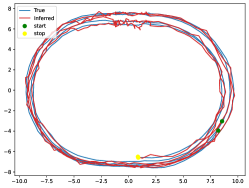
(a) RGPSSM

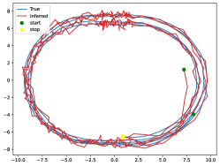
(b) SVMC

(c) OEnVI

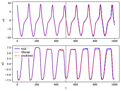
(d) RGPSSM (ours)

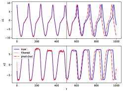
(e) SVMC [23]

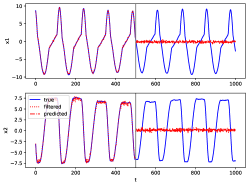
(f) OEnVI [18]

Figure 1: Online learning results for NASCAR^® dynamics. Top: filtered state trajectory; Bottom: filtering and prediction.

TABLE I: Prediction Accuracy and Computational Efficiency of the Three Online GPSSM Methods.

Method	RGPSSM	SVMC	OEnVI
Prediction RMSE	1.2552	5.9180	7.8583
Running Time (s)	8.59	42.69	6.55

V-B Synthetic Wing Rock Dynamics Learning

To further evaluate RGPSSM’s ability to online adapt GP hyperparameters and inducing points, it is tested on the synthetic wing rock dynamics learning task. In aerospace engineering, wing rock dynamics can cause roll oscillations in slender delta-winged aircraft, posing a significant threat to flight safety. To address this issue, most approaches rely on online learning of wing rock dynamics [34]. The associated dynamical system can be expressed by the following continuous-time SSM:

$$\dot{\theta} =p$$ (31)

$$\dot{p} =L_{\delta_{a}}\delta_{a}+\Delta(\theta,p)$$

where $\theta,p\in\mathbb{R}$ denote the roll angle and roll rate, respectively. As illustrated in (31), the dynamics model consists of a known part $L_{\delta_{a}}\delta_{a}$, where $\delta_{a}$ is the aileron control input and $L_{\delta_{a}}=3$, and an unknown uncertainty model $\Delta(\theta,p)$. The uncertainty model used in the simulation is taken from [34], namely:

$$\Delta(\theta,p) =W_{0}+W_{1}\theta+W_{2}p$$ (32)

$$\,+W_{3}|\theta|p+W_{4}|p|p+W_{5}\theta^{2}$$

where $W_{0}=0.8,W_{1}=0.2314,W_{2}=0.6918,W_{3}=-0.6245,W_{4}=0.0095,W_{5}=0.0214$. To further demonstrate the learning capacity of the proposed method under sparse sensor conditions, the measurement is limited to the roll angle $\theta$, which is corrupted by Gaussian white noise with a standard deviation of 0.2 degrees.

To apply the proposed method to learn wing rock dynamics, we specify a GP prior on the uncertainty model $\Delta(\theta,p)$ and then apply Algorithm 1 to the discretized-time form of (31). For hyperparameter adaptation, an iteration of hyperparameter optimization is performed in each RGPSSM update with a learning rate of 0.01. Additionally, the budget for inducing points is set to 20. In the following, we test the proposed method under these conditions and evaluate the effects of hyperparameter and inducing point adaptation.

Firstly, we conduct a Monte Carlo test of the proposed learning algorithm with different initial values of GP hyperparameters. The simulation results are depicted in Fig. 2 and 3. As shown in Fig. 2, all three GP hyperparameters gradually converge near the reference values, which are obtained through offline GP training using data pairs $(\theta,p,\Delta)$. In terms of learning accuracy, the prediction RMSE over the last 1/4 segment improves by 29.3% with hyperparameter adaptation. To more intuitively illustrate the benefits of hyperparameter adaptation, we present the state profile from one Monte Carlo simulation case, as shown in Fig. 3. In the figure, the blue solid lines depict the true values of state $\theta(t),p(t)$ and uncertainty $\Delta(t)$; the orange dashed lines represent the filtered state and uncertainty predictions obtained without hyperparameter adaptation; and the green dashed lines show the predictions with hyperparameter adaptation. It is evident that hyperparameter adaptation improves both the mean and variance predictions of the GP, thereby enhancing the filtering accuracy of the state, especially the roll rate $p$.

Secondly, to illustrate the adaptation process of the inducing points and their advantages, we present the associated results in Fig. 4. In this figure, the inducing inputs are represented by yellow diamonds, while the true state values are shown as white circles. It is evident that the number of inducing points gradually increases to the predefined budget, and the points are concentrated around the existing states. Given the localized nature of the SE kernel, this result indicates that the selected inducing points can effectively represent the GP model. Additionally, to assess learning accuracy, we use the background contour plot to visualize the distribution of prediction errors in the state space. It is evident that the prediction error decreases over time, particularly around the existing states, benefiting from the effective selection of inducing points.

Figure 2: Evolution of the GP hyperparameters during RGPSSM learning

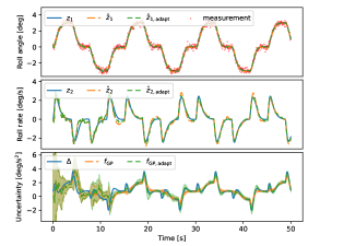
Figure 3: Evolution of the system states and their estimation, where the initial values of the GP hyperparameters are $l_{1}=l_{2}=5$ and $\sigma_{1}^{2}=10$. The shadows indicate 95% confidence intervals.

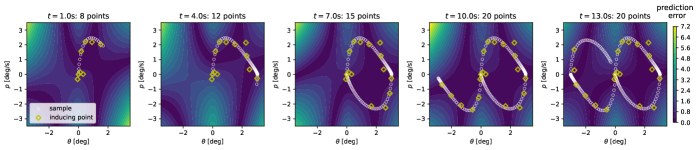
Figure 4: Evolution of inducing-point set and prediction error over time.

V-C Real-World System Identification Task

To evaluate the generalization capability of the proposed method, we conducted experiments on five real-world system identification benchmark datasets. The first half of each dataset was used for training, while the second half was reserved for testing predictive performance. Due to limited prior knowledge of the models and the restricted amount of training data, these datasets are mainly used for assessing offline GPSSM approaches. In this study, we performed an online learning experiment with the proposed method, comparing its performance against three state-of-the-art offline GPSSM techniques: PRSSM [14], VCDT [15], and EnVI [18]. For each method, the number of inducing points was capped at 20, and a 4-dimensional state GPSSM was used to capture system dynamics, with a transition model defined as $\boldsymbol{x}_{t+1}=f(\boldsymbol{x}_{t},u_{t+1})$, where $\boldsymbol{x}_{t}\in\mathbb{R}^{4}$, and a measurement model given by $y_{t}=[1,0,0,0]\boldsymbol{x}_{t}$. In addition, to activate the estimation for the latent state within RGPSSM, we randomly assign an inducing point around the origin before learning to make the transition Jacobian $A_{x}$ non-zero for each state dimension (see our code for details). The experimental results involving multiple simulations with different random seeds are summarized in Table II. As shown in the table, although online learning is challenging, the proposed method achieves the best prediction accuracy in three datasets, which is mainly due to the explicit consideration of the dependence between the system state and the GP, as shown in (8). These findings underscore the method’s robustness and ability to generalize across diverse datasets.

TABLE II: Performance Comparison of Different GPSSM Methods across Five System Identification Benchmarks. Prediction RMSE is Averaged over Five Seeds, with Standard Deviations Reported in Parentheses.

Methods	Offline			Online
	PRSSM	VCDT	EnVI	RGPSSM
Actuator	0.691 (0.148)	0.815 (0.012)	0.657 (0.095)	1.048 (0.142)
Ball Beam	0.074 (0.010)	0.065 (0.005)	0.055 (0.002)	0.046 (0.002)
Drive	0.647 (0.057)	0.735 (0.005)	0.703 (0.050)	0.863 (0.083)
Dryer	0.174 (0.013)	0.667 (0.266)	0.125 (0.017)	0.105 (0.004)
Gas Furnace	1.503 (0.196)	2.052 (0.163)	1.388 (0.123)	1.373 (0.061)

VI Conclusion

In this paper, we propose a novel recursive learning method, RGPSSM, for online inference in Gaussian Process State Space Models (GPSSMs). First, to enable learning in any operating domain, we derive a two-step Bayesian update equation that does not rely on any GP approximation. The derivation incorporates a mild first-order linearization to address the inherent nonlinearity within GPSSMs. Second, to mitigate the computational burden imposed by the nonparametric nature of GPs, we introduce a dynamic inducing-point set adjustment algorithm, ensuring computational efficiency. Third, to eliminate the burden for offline tuning of GP hyperparameters, we develop an online optimization method that extracts measurement information from the approximate posterior distribution. Through extensive evaluations on a diverse set of real and synthetic datasets, we demonstrate the superior learning performance and adaptability of the proposed method. In the future, research may focus on improving the accuracy of the first-order linearization by using techniques such as the iterative Kalman filter, extending the method to handle non-Gaussian data likelihoods, and adapting it to process and measurement noise covariances, as well as time-varying dynamics.

Appendix A Score for Selection of Inducing Point

This section derives the score quantifying the accuracy loss for discarding an inducing point, which is achieved based on the KL divergence in (18). As shown in (18), $D_{1}$ is unrelated to the point to discard $u_{d}$. Therefore, only $D_{2}$ and $D_{3}$ need to be evaluated. Without loss of generality, suppose the index of the discarded point $u_{d}$ is $i_{d}=1$.

Firstly, for $D_{2}$, the log-term in the intergration is:

$$\log p(u_{d}|\boldsymbol{u}_{l}) =-\dfrac{1}{2}\log(2\pi)-\dfrac{1}{2}\log|\gamma_{d}|$$ (33)

$$\,-\dfrac{1}{2}(\boldsymbol{u}_{d}-\boldsymbol{k}_{dl}\boldsymbol{u}_{l})^{T}\gamma_{d}^{-1}(\boldsymbol{u}_{d}-\boldsymbol{k}_{dl}\boldsymbol{u}_{l})$$

where $\boldsymbol{k}_{dl}=\boldsymbol{K}_{dl}\boldsymbol{K}_{ll}^{-1}$ and $\gamma_{d}=\boldsymbol{K}_{dd}-\boldsymbol{K}_{dl}\boldsymbol{K}_{ll}^{-1}\boldsymbol{K}_{ld}$. Denote $\boldsymbol{Q}=\boldsymbol{K}_{uu}^{-1}$, and using the matrix inversion formula (see Appendix A of [30]), we have:

$$\gamma_{d} ={\boldsymbol{Q}_{dd}}^{-1}$$ (34)

$$\boldsymbol{k}_{dl} =-{\boldsymbol{Q}_{dd}}^{-1}\boldsymbol{Q}_{dl}$$

where $\boldsymbol{Q}_{dd}$ denotes the $i_{d}$th diagonal element of matrix $\boldsymbol{Q}$, and $\boldsymbol{Q}_{dl}$ denotes the $i_{d}$th row of $\boldsymbol{Q}$ with $\boldsymbol{Q}_{dd}$ removed.

Using (18), (33) and (34), the $u_{d}$ relevant term in $D_{2}$ is:

$$\tilde{D}_{2} =\dfrac{1}{2}\log|\boldsymbol{Q}_{dd}|-\dfrac{1}{2}\Delta$$ (35)

$$\Delta =\int q(\boldsymbol{u})(u_{d}-\boldsymbol{k}_{dl}\boldsymbol{u}_{l})^{T}\boldsymbol{Q}_{dd}(u_{d}-\boldsymbol{k}_{dl}\boldsymbol{u}_{l})\,\mathrm{d}\boldsymbol{u}$$

$$=\mathbb{E}_{q(\boldsymbol{u})}\left[\mathrm{tr}\left(\boldsymbol{Q}_{dd}(u_{d}-\boldsymbol{k}_{dl}\boldsymbol{u}_{l})(u_{d}-\boldsymbol{k}_{dl}\boldsymbol{u}_{l})^{T}\right)\right]$$

$$=\mathrm{tr}\left(\boldsymbol{Q}_{dd}\mathbb{E}_{q(\boldsymbol{u})}\left[(u_{d}-\boldsymbol{k}_{dl}\boldsymbol{u}_{l})(u_{d}-\boldsymbol{k}_{dl}\boldsymbol{u}_{l})^{T}\right]\right)$$

Let $\boldsymbol{\phi}=[1,-\boldsymbol{k}_{dl}]$, and then we have $u_{d}-\boldsymbol{k}_{dl}\boldsymbol{u}_{l}=\boldsymbol{\phi}\boldsymbol{u}$. Using (34), we further have:

$$\boldsymbol{\phi} =\begin{bmatrix}1&{\boldsymbol{Q}}_{dd}^{-1}\boldsymbol{Q}_{dl}\\ \end{bmatrix}$$ (36)

$$=\begin{bmatrix}{\boldsymbol{Q}}_{dd}^{-1}\boldsymbol{Q}_{dd}&{\boldsymbol{Q}}_{dd}^{-1}\boldsymbol{Q}_{dl}\\ \end{bmatrix}$$

$$={\boldsymbol{Q}}_{dd}^{-1}\boldsymbol{Q}_{du}$$

where $\boldsymbol{Q}_{du}$ denotes the $i_{d}$th row of $\boldsymbol{Q}$. Therefore:

$$\Delta =\mathrm{tr}\left(\boldsymbol{Q}_{dd}\mathbb{E}_{q(\boldsymbol{u})}\left[\boldsymbol{\phi}\boldsymbol{u}\boldsymbol{u}^{T}\boldsymbol{\phi}^{T}\right]\right)$$ (37)

$$=\mathrm{tr}\left(\boldsymbol{Q}_{dd}\left[\boldsymbol{\phi}(\boldsymbol{S}_{uu}+\boldsymbol{m}_{u}\boldsymbol{m}_{u}^{T})\boldsymbol{\phi}^{T}\right]\right)$$

$$=\Delta_{1}+\Delta_{2}$$

where

$$\Delta_{1} =\boldsymbol{m}_{u}^{T}\boldsymbol{Q}_{du}^{T}{\boldsymbol{Q}}_{dd}^{-1}\boldsymbol{Q}_{du}\boldsymbol{m}_{u}$$ (38)

$$\Delta_{2} =\mathrm{tr}\left(\boldsymbol{Q}_{du}\boldsymbol{S}_{uu}\boldsymbol{Q}_{du}^{T}{\boldsymbol{Q}}_{dd}^{-1}\right)$$

For $D_{3}$, we can use the differential entropy identical for Gaussian distribution:

$$\int p(\boldsymbol{a})\log p(\boldsymbol{a})=-\dfrac{1}{2}\left[n_{a}+n_{a}\log(2\pi)+\log|\boldsymbol{\Sigma}_{a}|\right]$$ (39)

where $p(\boldsymbol{a})$ is a $n_{a}$-dimension Gaussian distribution with covariance $\boldsymbol{\Sigma}_{a}$. Deonte the covariance of joint distribution $q(\boldsymbol{X}_{t})$ that marginal out $u_{d}$ as $\boldsymbol{\Sigma}_{t,l}$, and deonte the inversion of orignial covariance as $\boldsymbol{\Omega}=\boldsymbol{\Sigma}_{t}^{-1}$. Then, given (39), the $u_{d}$ relevant term in $D_{3}$ is:

$$-\dfrac{1}{2}\log|\boldsymbol{\Sigma}_{t,l}| =-\dfrac{1}{2}\log\left(|\boldsymbol{\Sigma}_{t}|/|\boldsymbol{S}_{dd}-\boldsymbol{\zeta}_{d}^{T}\boldsymbol{\Sigma}_{t,l}\boldsymbol{\zeta}_{d}|\right)$$ (40)

$$=-\dfrac{1}{2}\log|\boldsymbol{\Sigma}_{t}|-\dfrac{1}{2}\log|\boldsymbol{\Omega}_{dd}|$$

$$\boldsymbol{\zeta}_{d} =\begin{bmatrix}\boldsymbol{V}_{xd}\\ \boldsymbol{S}_{ud}\\ \end{bmatrix}$$

where $\boldsymbol{\Omega}_{dd}$ is the element of the matrix $\boldsymbol{\Omega}$ corresponding to the discarded point $u_{d}$, namely, its $(n_{x}+i_{d})$-th diagonal element. In addition, (40) is dervied by using the properties of the determinants of block matrices and the matrix inversion formula (see Appendix A of [30]).

Based on the KL divergence (18) and combing (35), (38) and (40), we have the scroe:

$$s_{d}=\Delta_{1}+\Delta_{2}+\Delta_{3}$$ (41)

where

$$\Delta_{3}=\log|\boldsymbol{\Omega}_{dd}|-\log|\boldsymbol{Q}_{dd}|$$ (42)

In terms of effect, a lower value of the score $s_{d}$ implies less accuracy loss for discarding the point $u_{d}$.

Appendix B Prediction Equation without Adding Points

According to (17), if the new inducing point $f_{t}$ is discarded in the prediction step, the distribution after discarding can be given by:

$$\hat{q}^{*}(\boldsymbol{x}_{t+1},\boldsymbol{u}) =\int q^{-}(\boldsymbol{x}_{t+1},\bar{\boldsymbol{u}})\mathrm{d}f_{t}$$ (43)

Then, by incorporating the original prediction equation (12), we have:

$$\hat{q}^{*}(\boldsymbol{x}_{t+1},\boldsymbol{u}) =\int\int\hat{p}(\boldsymbol{x}_{t+1}|\boldsymbol{x}_{t},f_{t})\,q(\boldsymbol{x}_{t},\bar{\boldsymbol{u}})\,\mathrm{d}\boldsymbol{x}_{t}\,\mathrm{d}f_{t}$$ (44)

$$=\int\int\hat{p}(\boldsymbol{x}_{t+1}|\boldsymbol{x}_{t},f_{t})\,p(f_{t}|\boldsymbol{u})\,q(\boldsymbol{x}_{t},\boldsymbol{u})\,\mathrm{d}\boldsymbol{x}_{t}\,\mathrm{d}f_{t}$$

$$=\int\hat{p}(\boldsymbol{x}_{t+1}|\boldsymbol{x}_{t},\boldsymbol{u})\,q(\boldsymbol{x}_{t},\boldsymbol{u})\,\mathrm{d}\boldsymbol{x}_{t}$$

where $\hat{p}(\boldsymbol{x}_{t+1}|\boldsymbol{x}_{t},\boldsymbol{u})$ represents a new transition model, whose specific expression is:

$$\hat{p}(\boldsymbol{x}_{t+1}|\boldsymbol{x}_{t},\boldsymbol{u})$$ (45)

$$=\int\hat{p}(\boldsymbol{x}_{t+1}|\boldsymbol{x}_{t},f_{t})\,p(f_{t}|\boldsymbol{u})\,\mathrm{d}f_{t}$$

$$=\int\hat{p}(\boldsymbol{x}_{t+1}|\boldsymbol{x}_{t},f_{t})\,\mathcal{N}(f_{t}|\boldsymbol{k}_{tu}\boldsymbol{u},\gamma)\,\mathrm{d}f_{t}$$

$$=\mathcal{N}\Big{(}\boldsymbol{x}_{t+1}\Big{|}\boldsymbol{F}_{t}+\boldsymbol{A}_{x}(\boldsymbol{x}_{t}-\boldsymbol{\mu}_{t})+\boldsymbol{A}_{f}\boldsymbol{k}_{tu}(\boldsymbol{u}-\boldsymbol{m}_{u}),\tilde{\boldsymbol{\Sigma}}_{f}\Big{)}$$

where $\gamma=\boldsymbol{K}_{tt}-\boldsymbol{K}_{tu}\boldsymbol{K}_{uu}^{-1}\boldsymbol{K}_{ut}$ and $\tilde{\boldsymbol{\Sigma}}_{f}=\boldsymbol{A}_{f}\gamma\boldsymbol{A}_{f}^{T}+\boldsymbol{\Sigma}_{f}$.

Combining (44) and (45), the prediction equation (21) can be obtained.

Appendix C Derivation Details of GP Hyperparameters Optimization

This section derives the moments of the approximate joint distribution $q_{new}(\boldsymbol{x}_{t},\boldsymbol{f})$ in (26), along with the optimizing objective for GP hyperparameters.

Firstly, to derive the moments of the approximate joint distribution $q_{new}(\boldsymbol{x}_{t},\boldsymbol{f})$, we can utilize the following result:

$$\dfrac{p(\boldsymbol{u};\boldsymbol{\theta}_{new})}{p(\boldsymbol{u};\boldsymbol{\theta}_{old})} =\dfrac{\mathcal{N}(\boldsymbol{u}|\boldsymbol{0},\boldsymbol{K}_{uu}^{new})}{\mathcal{N}(\boldsymbol{u}|\boldsymbol{0},\boldsymbol{K}_{uu}^{old})}$$ (46)

$$=Z\mathcal{N}(\boldsymbol{u}|\boldsymbol{0},\Delta\boldsymbol{K})$$

$$=Z\mathcal{N}(\boldsymbol{0}|\boldsymbol{u},\Delta\boldsymbol{K})$$

where

$$\Delta\boldsymbol{K} =[(\boldsymbol{K}_{uu}^{new})^{-1}-(\boldsymbol{K}_{uu}^{old})^{-1}]^{-1}$$ (47)

$$Z \propto\dfrac{|\boldsymbol{K}_{uu}^{old}|^{1/2}|\Delta\boldsymbol{K}|^{1/2}}{|\boldsymbol{K}_{uu}^{new}|^{1/2}}$$

Note that, the above equations hold only in a mathematical sense and does not have probabilistic meaning, as $\Delta\boldsymbol{K}$ may not be positive definite. Combining (26) and (46), we have:

$$q_{new}(\boldsymbol{x}_{t},\boldsymbol{u})\propto\mathcal{N}(\boldsymbol{0}|\boldsymbol{u},\Delta\boldsymbol{K})q_{old}(\boldsymbol{x}_{t},\boldsymbol{u})$$ (48)

whose moments can be obtained by the correction eqution of Kalman filter:

$$\tilde{\boldsymbol{H}}=\begin{bmatrix}\boldsymbol{0}&\boldsymbol{I}_{n_{u}}\\ \end{bmatrix}$$ (49)

$$\tilde{\boldsymbol{G}}=\boldsymbol{\Sigma}_{t}^{old}\tilde{\boldsymbol{H}}^{T}\left(\boldsymbol{S}_{uu}^{old}+\Delta\boldsymbol{K}\right)^{-1}$$

$$\boldsymbol{\xi}_{t}^{new}=\boldsymbol{\xi}_{t}^{old}-\tilde{\boldsymbol{G}}\boldsymbol{\xi}_{t}^{old}$$

$$\boldsymbol{\Sigma}_{t}^{new}=\boldsymbol{\Sigma}_{t}^{old}-\tilde{\boldsymbol{G}}\tilde{\boldsymbol{H}}\boldsymbol{\Sigma}_{t}^{old}$$

where $\boldsymbol{\xi}_{t}$ and $\boldsymbol{\Sigma}_{t}$ represents the mean and covariance of the augmented state $\boldsymbol{X}_{t}=[\boldsymbol{x}_{t}^{T},\boldsymbol{u}^{T}]^{T}$.

Secondly, in order to optimize the GP hyperparameters, considering (27) and (46), we can maximize:

$$\log\dfrac{p(\boldsymbol{y}_{1:t};\boldsymbol{\theta}_{new})}{p(\boldsymbol{y}_{1:t};\boldsymbol{\theta}_{old})}$$ (50)

$$=\log\int Z\mathcal{N}(\boldsymbol{0}|\boldsymbol{u},\Delta\boldsymbol{K})q_{old}(\boldsymbol{x}_{t},\boldsymbol{u})\,\mathrm{d}\boldsymbol{x}_{t}\,\mathrm{d}\boldsymbol{u}$$

$$=\log\mathcal{N}(\boldsymbol{0}|\boldsymbol{m}_{u}^{old},\Delta\boldsymbol{K}+\boldsymbol{S}_{uu}^{old})+\log Z$$

Then, by dropping some $\boldsymbol{\theta}_{new}$-irrelevant terms, the optimization objective can be transformed to minimize:

$$\mathcal{L} =\mathcal{L}_{1}+\mathcal{L}_{2}$$ (51)

where

$$\mathcal{L}_{1} =(\boldsymbol{m}_{u}^{old})^{T}(\boldsymbol{S}_{uu}^{old}+\Delta\boldsymbol{K})^{-1}\boldsymbol{m}_{u}^{old}$$ (52)

$$\mathcal{L}_{2} =-\log|\Delta\boldsymbol{K}|+\log|\boldsymbol{K}_{uu}^{new}|+\log|\Delta\boldsymbol{K}+\boldsymbol{S}_{uu}^{old}|$$

$$=\log|\boldsymbol{K}_{uu}^{new}|+\log|\boldsymbol{I}_{n_{u}}+\Delta\boldsymbol{K}^{-1}\boldsymbol{S}_{uu}^{old}|$$

$$=\log|\boldsymbol{K}_{uu}^{new}+[\boldsymbol{I}_{n_{u}}-\boldsymbol{K}_{uu}^{new}(\boldsymbol{K}_{uu}^{old})^{-1}]\boldsymbol{S}_{uu}^{old}|$$

Here, we avoid the appearance of $\Delta\boldsymbol{K}$ in the loss function through some operations, because when $\boldsymbol{K}_{uu}^{new}=\boldsymbol{K}_{uu}^{old}$, $\Delta\boldsymbol{K}$ is not well-defined.

Appendix D Stable Implementation Method

To solve the numerical stability problem in RGPSSM, this section develops a stable implementation method based on Cholesky decomposition. Specifically, the covariance $\boldsymbol{\Sigma}_{t}$ of the augmented state $\boldsymbol{X}_{t}$ is decomposed as $\boldsymbol{\Sigma}_{t}=\boldsymbol{L}_{t}\boldsymbol{L}_{t}^{T}$, where $\boldsymbol{L}_{t}$ is a lower triangular matrix, known as the Cholesky factor. Based on this decomposition, the evolution of the covariance $\boldsymbol{\Sigma}_{t}$ is replaced by the evolution of the Cholesky factor, which can reduce the accumulation of computational rounding errors. To implement this method, we must modify the moment update equations within the prediction and correction steps, as well as during the discarding of inducing points and hyperparameter optimization.

For the prediction step, there exist two cases: not adding points and adding points. Firstly, for the prediction equation without adding points (21), the covariance update can be rewritten by:

$$\boldsymbol{\Sigma}_{t+1}^{-} =\begin{bmatrix}\boldsymbol{\Phi}_{t}\boldsymbol{L}_{t}&\boldsymbol{D}_{f}\\ \end{bmatrix}\begin{bmatrix}\boldsymbol{L}_{t}^{T}\boldsymbol{\Phi}_{t}^{T}\\ \boldsymbol{D}_{f}^{T}\\ \end{bmatrix}$$ (53)

where $\boldsymbol{D}_{f}$ is the Cholesky factor of the process noise covariance $\boldsymbol{\Sigma}_{f,\boldsymbol{X}}$. Then, through the following QR decomposition:

$$\begin{bmatrix}\boldsymbol{L}_{t}^{T}\boldsymbol{\Phi}_{t}^{T}\\ \boldsymbol{D}_{f}^{T}\\ \end{bmatrix}=\boldsymbol{O}\boldsymbol{R}$$ (54)

where $\boldsymbol{O}$ is an orthogonal matrix and $\boldsymbol{R}$ is an upper triangular matrix, we can obtain the Cholesky factor of the predicted covariance $\boldsymbol{\Sigma}^{-}_{t+1}$, namely, $\boldsymbol{L}_{t+1}^{-}=\boldsymbol{R}^{T}$.

Then, for the case of prediction with adding points, it involves one additional step: evaluating the Cholesky factor $\bar{\boldsymbol{L}}_{t}$ of the augmented covariance $\bar{\boldsymbol{\Sigma}}_{t}$ after adding a point. According to the definition, the augmented covariance $\bar{\boldsymbol{\Sigma}}_{t}$ can be expressed as follows:

$$\bar{\boldsymbol{\Sigma}}_{t}=\begin{bmatrix}\boldsymbol{\Sigma}_{t}&\boldsymbol{\zeta}_{t}\\ \boldsymbol{\zeta}_{t}^{T}&\boldsymbol{S}_{tt}\\ \end{bmatrix},\quad\boldsymbol{\zeta}_{t}=\begin{bmatrix}\boldsymbol{V}_{xt}\\ \boldsymbol{S}_{ut}\\ \end{bmatrix}$$ (55)

In view of this expression, we can define:

$$\bar{\boldsymbol{L}}_{t}=\begin{bmatrix}\boldsymbol{L}_{t}&\boldsymbol{0}\\ \boldsymbol{\alpha}&\boldsymbol{\beta}\\ \end{bmatrix}$$ (56)

and correspondingly we have:

$$\bar{\boldsymbol{\Sigma}}_{t}=\begin{bmatrix}\boldsymbol{L}_{t}\boldsymbol{L}_{t}^{T}&\boldsymbol{L}_{t}\boldsymbol{\alpha}^{T}\\ \boldsymbol{\alpha}^{T}\boldsymbol{L}_{t}^{T}&\boldsymbol{\alpha}\boldsymbol{\alpha}^{T}+\boldsymbol{\beta}\boldsymbol{\beta}^{T}\\ \end{bmatrix}$$ (57)

Combining (55) and (57), we can obtain $\boldsymbol{\alpha}$ by solving the linear equation $\boldsymbol{L}_{t}\boldsymbol{\alpha}^{T}=\boldsymbol{\zeta}_{t}$, and then compute $\boldsymbol{\beta}=\mathrm{cholesky}\left(\boldsymbol{S}_{tt}-\boldsymbol{\alpha}\boldsymbol{\alpha}^{T}\right)$, thus obtaining the Cholesky factor $\bar{\boldsymbol{L}}_{t}$. Then, similar operations as in (53) and (54) can be implemented to evaluate the predicted Cholesky factor.

For the correction step, given (16), the update equation for covariance can be rewritten as:

$$\boldsymbol{\Sigma}_{t+1} =\boldsymbol{\Sigma}_{t+1}^{-}-\boldsymbol{\Sigma}_{t+1}^{-}\boldsymbol{H}^{T}(\boldsymbol{C}\boldsymbol{P}_{t+1}^{-}\boldsymbol{C}^{T}+\boldsymbol{\Sigma}_{g})^{-1}\boldsymbol{H}\boldsymbol{\Sigma}_{t+1}^{-}$$ (58)

$$=\boldsymbol{\Sigma}_{t+1}^{-}-\boldsymbol{\Sigma}_{t+1}^{-}\boldsymbol{H}^{T}(\boldsymbol{\rho}\boldsymbol{\rho}^{T})^{-1}\boldsymbol{H}\boldsymbol{\Sigma}_{t+1}^{-}$$

$$=\boldsymbol{L}_{t+1}^{-}\boldsymbol{L}_{t+1}^{-T}-\boldsymbol{\eta}\boldsymbol{\eta}^{T}$$

where $\boldsymbol{\rho}=\mathrm{cholesky}(\boldsymbol{C}\boldsymbol{P}_{t+1}^{-}\boldsymbol{C}^{T}+\boldsymbol{\Sigma}_{g})$ and $\boldsymbol{\eta}=\boldsymbol{\Sigma}_{t+1}^{-}\boldsymbol{H}^{T}(\boldsymbol{\rho}^{-1})^{T}$. Considering (58), we can evaluate the Cholesky factor $\boldsymbol{L}_{t+1}$ of the posterior covariance $\boldsymbol{\Sigma}_{t+1}$ using the Cholesky downdate algorithm (See Section 6.5.4 of [35]), namely, $\boldsymbol{L}_{t+1}=\mathrm{choldowndate}(\boldsymbol{L}_{t+1}^{-},\boldsymbol{\eta})$.

For discarding an inducing point, to evaluate the updated Cholesky factor, we can express the original Cholesky factor before discarding as follows:

$$\boldsymbol{L}_{t}=\begin{bmatrix}\boldsymbol{A}&\boldsymbol{0}&\boldsymbol{0}\\ \boldsymbol{a}&\boldsymbol{b}&\boldsymbol{0}\\ \boldsymbol{B}&\boldsymbol{c}&\boldsymbol{C}\end{bmatrix}$$ (59)

Here, we reuse the notation $\boldsymbol{A},\boldsymbol{B},\boldsymbol{C},\boldsymbol{a},\boldsymbol{b},\boldsymbol{c}$, where $\boldsymbol{a},\boldsymbol{b},\boldsymbol{c}$ denote the blocks corresponding to the discarded point $u_{d}$. Given (17), the updated covariance $\boldsymbol{\Sigma}_{t}^{\prime}$ is the original one with the $i_{d}$th row and $i_{d}$th column removed, which can be given using the expression in (59):

$$\boldsymbol{\Sigma}_{t}^{\prime}=\begin{bmatrix}\boldsymbol{A}\boldsymbol{A}^{T}&\boldsymbol{A}\boldsymbol{B}^{T}\\ \boldsymbol{B}\boldsymbol{A}^{T}&\boldsymbol{B}\boldsymbol{B}^{T}+\boldsymbol{c}\boldsymbol{c}^{T}+\boldsymbol{C}\boldsymbol{C}^{T}\\ \end{bmatrix}$$ (60)

In view of this expression, the updated Cholesky factor $\boldsymbol{L}_{t}^{\prime}$ can be given by:

$$\boldsymbol{L}_{t}^{\prime}=\begin{bmatrix}\boldsymbol{A}&\boldsymbol{0}\\ \boldsymbol{B}&\mathrm{cholupdate}(\boldsymbol{C},\boldsymbol{c})\\ \end{bmatrix}$$ (61)

where $\mathrm{cholupdate}(\cdot,\cdot)$ denotes the Cholesky update algorithm (see Section 6.5.4 of [35]), namely a efficient method for evaluating the Cholesky factor of $(\boldsymbol{c}\boldsymbol{c}^{T}+\boldsymbol{C}\boldsymbol{C}^{T})$.

For hyperparameter optimization, since $\Delta\boldsymbol{K}$ in (29) may not be positive definite as illustrated in Appendix C, we cannot update the Cholesky factor as in the correction step. Therefore, the updated Cholesky factor is evaluated by directly decomposing the updated covariance $\boldsymbol{\Sigma}_{t}^{\text{new}}$, which is obtained using (29).

Overall, the Cholesky versions of the update equations in the prediction and correction steps, as well as for discarding inducing points and optimizing hyperparameters, have been derived, which makes the computations more compact, thereby enhancing numerical stability.

References

- [1] Y. Wu, J. M. Hernández-Lobato, and Z. Ghahramani, “Gaussian process volatility model,” Advances in neural information processing systems, vol. 27, 2014.
- [2] M. Dowling, “Approximate bayesian inference for state-space models of neural dynamics,” Ph.D. dissertation, State University of New York at Stony Brook, 2023.
- [3] C. Veibäck, J. Olofsson, T. R. Lauknes, and G. Hendeby, “Learning target dynamics while tracking using gaussian processes,” IEEE Transactions on Aerospace and Electronic Systems, vol. 56, no. 4, pp. 2591–2602, 2019.
- [4] A. J. McHutchon et al., “Nonlinear modelling and control using gaussian processes,” Ph.D. dissertation, Citeseer, 2015.
- [5] S. S. Rangapuram, M. W. Seeger, J. Gasthaus, L. Stella, Y. Wang, and T. Januschowski, “Deep state space models for time series forecasting,” Advances in neural information processing systems, vol. 31, 2018.
- [6] D. Gedon, N. Wahlström, T. B. Schön, and L. Ljung, “Deep state space models for nonlinear system identification,” IFAC-PapersOnLine, vol. 54, no. 7, pp. 481–486, 2021.
- [7] R. Frigola, “Bayesian time series learning with gaussian processes,” Ph.D. dissertation, 2015.
- [8] R. Turner, M. Deisenroth, and C. Rasmussen, “State-space inference and learning with gaussian processes,” in Proceedings of the thirteenth international conference on artificial intelligence and statistics. JMLR Workshop and Conference Proceedings, 2010, pp. 868–875.
- [9] J. F. Fisac, A. K. Akametalu, M. N. Zeilinger, S. Kaynama, J. Gillula, and C. J. Tomlin, “A general safety framework for learning-based control in uncertain robotic systems,” IEEE Transactions on Automatic Control, vol. 64, no. 7, pp. 2737–2752, 2018.
- [10] R. Frigola, F. Lindsten, T. B. Schön, and C. E. Rasmussen, “Bayesian inference and learning in gaussian process state-space models with particle mcmc,” Advances in neural information processing systems, vol. 26, 2013.
- [11] R. Frigola, Y. Chen, and C. E. Rasmussen, “Variational gaussian process state-space models,” Advances in neural information processing systems, vol. 27, 2014.
- [12] A. Svensson and T. B. Schön, “A flexible state–space model for learning nonlinear dynamical systems,” Automatica, vol. 80, pp. 189–199, 2017.
- [13] S. Eleftheriadis, T. Nicholson, M. Deisenroth, and J. Hensman, “Identification of gaussian process state space models,” Advances in neural information processing systems, vol. 30, 2017.
- [14] A. Doerr, C. Daniel, M. Schiegg, N.-T. Duy, S. Schaal, M. Toussaint, and T. Sebastian, “Probabilistic recurrent state-space models,” in International conference on machine learning. PMLR, 2018, pp. 1280–1289.
- [15] A. D. Ialongo, M. Van Der Wilk, J. Hensman, and C. E. Rasmussen, “Overcoming mean-field approximations in recurrent gaussian process models,” in International Conference on Machine Learning. PMLR, 2019, pp. 2931–2940.
- [16] J. Lindinger, B. Rakitsch, and C. Lippert, “Laplace approximated gaussian process state-space models,” in Uncertainty in Artificial Intelligence. PMLR, 2022, pp. 1199–1209.
- [17] X. Fan, E. V. Bonilla, T. O’Kane, and S. A. Sisson, “Free-form variational inference for gaussian process state-space models,” in International Conference on Machine Learning. PMLR, 2023, pp. 9603–9622.
- [18] Z. Lin, Y. Sun, F. Yin, and A. H. Thiéry, “Ensemble kalman filtering meets gaussian process ssm for non-mean-field and online inference,” IEEE Transactions on Signal Processing, 2024.
- [19] C. E. Rasmussen and C. K. I. Williams, Gaussian Processes for Machine Learning, 3rd ed., ser. Adaptive Computation and Machine Learning. MIT Press.
- [20] A. Kullberg, I. Skog, and G. Hendeby, “Learning driver behaviors using a gaussian process augmented state-space model,” in 2020 IEEE 23rd International Conference on Information Fusion (FUSION), pp. 1–7. [Online]. Available: https://ieeexplore.ieee.org/abstract/document/9190245
- [21] A. Kullberg, “On joint state estimation and model learning using gaussian process approximations,” Ph.D. dissertation, Linköping University Electronic Press, 2021.
- [22] K. Berntorp, “Online bayesian inference and learning of gaussian-process state–space models,” Automatica, vol. 129, p. 109613, 2021.
- [23] Y. Zhao, J. Nassar, I. Jordan, M. Bugallo, and I. M. Park, “Streaming variational monte carlo,” IEEE transactions on pattern analysis and machine intelligence, vol. 45, no. 1, pp. 1150–1161, 2022.
- [24] Y. Liu, M. Ajirak, and P. M. Djurić, “Sequential estimation of gaussian process-based deep state-space models,” IEEE Transactions on Signal Processing, 2023.
- [25] A. Doucet, A. M. Johansen et al., “A tutorial on particle filtering and smoothing: Fifteen years later,” Handbook of nonlinear filtering, vol. 12, no. 656-704, p. 3, 2009.
- [26] S.-S. Park, Y.-J. Park, Y. Min, and H.-L. Choi, “Online gaussian process state-space model: Learning and planning for partially observable dynamical systems,” International Journal of Control, Automation and Systems, vol. 20, no. 2, pp. 601–617, 2022.
- [27] M. O’Connell, G. Shi, X. Shi, K. Azizzadenesheli, A. Anandkumar, Y. Yue, and S.-J. Chung, “Neural-fly enables rapid learning for agile flight in strong winds,” Science Robotics, vol. 7, no. 66, p. eabm6597, 2022.
- [28] S. Van Vaerenbergh, M. Lázaro-Gredilla, and I. Santamaría, “Kernel recursive least-squares tracker for time-varying regression,” IEEE transactions on neural networks and learning systems, vol. 23, no. 8, pp. 1313–1326, 2012.
- [29] L. Csató and M. Opper, “Sparse on-line gaussian processes,” Neural computation, vol. 14, no. 3, pp. 641–668, 2002.
- [30] L. Csató, “Gaussian processes: iterative sparse approximations,” Ph.D. dissertation, Citeseer, 2002.
- [31] T. D. Bui, C. Nguyen, and R. E. Turner, “Streaming sparse gaussian process approximations,” Advances in Neural Information Processing Systems, vol. 30, 2017.
- [32] D. P. Kingma, “Adam: A method for stochastic optimization,” arXiv preprint arXiv:1412.6980, 2014.
- [33] S. Linderman, M. Johnson, A. Miller, R. Adams, D. Blei, and L. Paninski, “Bayesian learning and inference in recurrent switching linear dynamical systems,” in Artificial intelligence and statistics. PMLR, 2017, pp. 914–922.
- [34] G. Chowdhary, H. A. Kingravi, J. P. How, and P. A. Vela, “Bayesian nonparametric adaptive control using gaussian processes,” IEEE transactions on neural networks and learning systems, vol. 26, no. 3, pp. 537–550, 2014.
- [35] G. H. Golub and C. F. Van Loan, Matrix computations. JHU press, 2013.