[table]capposition=top

Hydrodynamics of fault gouges from constitutive modelling to the physics of friction

Abstract

The development of rate- and state-dependent friction laws offered important insights into the key physical mechanisms of the frictional behaviour of fault gouges and their seismic cycle. However, past approaches were specifically tailored to address the problem of fault shearing, leaving questions about their ability to comprehensively represent the gouge material under general loading conditions. This work establishes an alternative approach for developing a physical friction law for fault gouges that is grounded on the rigour of the hydrodynamic procedure with two-scale temperatures through Terracotta, a thoroughly robust constitutive model for clay in triaxial loading conditions. By specifying the model for direct shearing, the approach yields an alternative friction law that readily captures the frictional dynamics of fault gouges, including explicit dependencies on gouge layer thickness, normal stress, and solid fraction. Validated against available laboratory experiments, the friction law retains the original predictive capabilities of Terracotta in triaxial conditions and explains the rate- and state-dependent, dilatational behaviour of fault gouges in direct shear conditions. Finally, when the Terracotta friction law is connected to a spring-dashpot representation of the host rock, the combined model predicts an elastic buildup precursor to the onset of and subsequent seismicity, with results closely reflecting experimental evidence and field observations. While this study focuses on clay-rich gouges, the approach and findings are expected to offer much wider implications to a variety of materials.

1   Introduction

Over recent decades, experimental and modelling efforts have focused on representing the frictional behaviour of faults to deepen our understanding of seismogenesis and the seismic cycle. Laboratory tests on rock, clay, and granular fault gouges have motivated the development of rate-and-state friction laws Dieterich (1979); Ruina (1983); Marone (1998); Saffer  Marone (2003), which aim to describe key features of earthquake nucleation and occurrence. Originally developed to phenomenologically capture the frictional and healing behaviour observed in laboratory tests Dieterich (1979), these friction laws have been instrumental in linking experimental data with the mechanics of earthquakes and faulting <e.g.,¿scholz2019mechanics. Rate-and-state frictional parameters are generally obtained through fitting the friction law to curves obtained from velocity stepping or slide-hold-slide friction experiments Marone (1998); Saffer  Marone (2003). The corresponding rate-and-state friction laws are conventionally adopted to model the mechanics of earthquakes and faulting, offering a robust explanation for numerous laboratory observations JC. Gu . (1984); Y. Gu  Wong (1991). Combined with continuum elasticity of the surrounding rock mass, these laws have also been applied to simulate natural and induced fault behaviours such as earthquake nucleation <e.g.,¿lapusta_rice_2000,scholz2019mechanics, aftershock sequences Marone . (1995); T. Chen  Lapusta (2009), and postseismic or interseismic fault creep and healing Marone (1998); Hetland . (2010).

Nevertheless, several limitations remain. The main challenge in using rate-and-state friction laws is the empirical nature of their parameters, which do not directly correspond to specific physical mechanisms. Consequently, existing rate-and-state friction laws cannot readily explain fault responses under diversely different laboratory and natural conditions without constant adaptation of the material constants <see¿spiers2016. In particular, earthquake nucleation and rupture propagation Rice  Ruina (1983); Tse  Rice (1986) depend considerably on factors such as temperature, stress level and slip velocity, which complicates the calibration of rate-and-state friction laws J. Chen  Spiers (2016); Bedford . (2022); Carpenter . (2014). These limitations of rate-and-state friction laws stem from two main factors: (1) their empirical foundation, which is based on a rather retrospective and idealised view of contact asperity behaviour, and (2) the fact they ignore the gouge volume within the fault, which does not only sustain shear sliding but also consolidation and shear-induced dilation processes <for further details, see¿spiers2016.

To address these limitations, recent effort has focused on the development of models inspired by physics at the microscale that capture steady-state and transient fault friction while grounding parameter constraints on micromechanics <among others, see¿niemeijer2007spiers,noda2008,spiers2016,ikarietal2016,Niemeijer2017,perfettini2017,van2018comparison. A pivotal development along this direction is the model by Chen, Niemeijer, and Spiers, also known as the CNS model, which incorporates deformation mechanisms at the microstructural level that differentiate between a localised shear band and a bulk gouge layer. With some adaptation, the model could further include normal stress effects on the frictional behaviour Yu . (2024). To achieve these feats, unlike phenomenological rate-and-state friction laws, the model does not ignore the dilatational shear of faults Makedonska . (2011).

While micromechanically-inspired fault models such as the CNS model have made significant strides, their ability to represent the response of the same gouge material under loading conditions that differ from direct fault shear has not been tested, leaving questions about the their ability to robustly represent the material. For example, a general physical model should be capable of representing the response of the same gouge material under isotropic loading, triaxial shear conditions, or even the dependence of fault friction on the reversal of the slip velocity that may happen during an earthquake. While specifically tailored for fault shearing, such cyclical conditions should engage gouge elasticity that is not accounted for in both rate-and-state and micromechanically-inspired friciton laws. Similarly, most existing fault friction laws tend to focus exclusively on inelastic slip behaviour, ignoring the initial elastic response of the material prior to the establishment of mature shear response. Therefore, the scope of these previous models cannot be easily extended to explain questions regarding the genesis of frictional faults. Finally, it is also important to note that these models have not fully addressed how the frictional behaviour depends on the thickness of the slip layer, despite experimental and in-situ evidence for this effect <e.g.,¿[among others]byerlee1976note, 93JB03361, 2011JB008264, evans1990thickness, JB095iB05p07007, einat2011friction,scuderi2014physicochemical, lyu2019mechanics, bedford2021role.

The objective of this work is the development of a new physics-based friction law for fault gouges that is grounded upon hydrodynamic principles. The key idea of this work lies in the philosophy of the development (see Figure 1). Instead of constructing a law directly by inspecting the specific loading conditions the gouge material sustains while the fault slides, we use an existing constitutive model for clay, originally developed for triaxial loading conditions that are different to those during fault sliding. This approach ensures that our results are objective and free from potential bias. The model named Terracotta, leverages the rigorous hydrodynamic procedure by landau2013statistical, which was developed originally for fluid continua. Later, this framework was extended to describe liquid crystals De Gennes  Prost (1993), granular media Jiang  Liu (2009), and partially saturated porous media Einav  Liu (2023), amongst other materials. Having been grounded upon hydrodynamic principles, Terracotta satisfies the first and second law of thermodynamics, momentum and mass balance laws Einav  Liu (2018), material objectivity, and the thermodynamic reciprocity of irreversible thermodynamic fluxes Onsager (1931), as well as considers the physical scale separation of temperatures in heterogeneous media and the energy flow in between Jiang  Liu (2009).

Building on the original Terracotta model for triaxial loading conditions, we first construct the tensorial generalisation of the model, while preserving all of its original physics and predictive triaxial features. Equipped with the tensorially generalised model, we move further by specifying the unique boundary conditions of an isolated fault gouge under direct shear loading. In so doing, we derive an alternative friction law that automatically preserves the model’s capacity to represent volumetric material response, including during consolidation and dilatational shear. The resulting physics-based friction law encapsulates the essential features of both rate-and-state and micromechanically-inspired friction laws while naturally introducing dependencies on key meaningful parameters and state variables.

The resulting Terracotta friction law incorporates several physical phenomena previously ignored by fault friction laws. For example, the model accurately represents the pressure- and density-dependent elasticity of gouge media, allowing it to simulate the buildup of an elastic stress, which fully lets it account for the effects of the total normal stress. The Terracotta friction law also builds on the concept of critical state in soil mechanics Wood (1990) and the thermodynamic reciprocity of plastic volumetric and deviatoric plastic straining Wiebicke  Einav (2024). The latter feature enhances the capability of the model to predict post-peak frictional behaviour, providing a physically grounded explanation for dilatational slip hardening and weakening. An important feature of the friction law is the consideration of a finite fault gouge thickness as a physical quantity. Its temporal evolution directly depends on the prescribed normal stress under direct shear boundary conditions, which also influences the elastic development of frictional instabilities. Consistent with the original Terracotta model Wiebicke  Einav (2024), the derived friction law accounts for the influence and evolution of the porosity (or alternatively, the solid fraction) of the gouge material. Another key ingredient is the inclusion of the meso-related temperature (from here, to be called meso-temperature) as a non-equilibrium variable for clay, rooted on prior developments for granular media Jiang  Liu (2009); Alaei . (2021). Unlike the conventional thermal temperature, which reflects atomic-scale thermal fluctuations, the meso-temperature captures the kinetic energy of the velocity fluctuations of the clay mesostructures, including the motion of platelets and aggregates that are overwhelmingly larger than atoms, thus attributed to have their own temperature. When stressed or deformed, these mesostructures exhibit fluctuations akin to granular particles, with pores expanding, collapsing, and clusters fragmenting. This motion at the mesoscale influences the material’s elasticity and viscosity, as depicted in Figure 1. Despite the advanced hydrodynamic procedure, the Terracotta friction law reveals a simple mathematical structure (as shall eventually be captured mathematically in Equation (22)).

Figure 1: Hydrodynamics of fault gouges: from constitutive to friction law. A fault gouge (a) subjected to tectonic movement with slip velocity $v_{\infty}$ is represented as (b) a slip layer of thickness $h$, subjected to an overburden stress $\sigma_{n}$, experiencing slip and normal velocities (known as rates), $v$ and $v_{n}$, that control the development of the shear stress $\tau$. The internal energy of the gouge is either held in the system through elastic stress, $\smash{\sigma^{e}_{ij}}$, or dissipated as a two-stage irreversible mechanism through the generation of thermal and meso-related entropy productions ($R$ and $R_{m}$) as functions of the plastic strain rate, $\smash{\dot{\varepsilon}^{p}_{ij}}$, and the viscous stress, $\smash{\sigma^{d}_{ij}}$, both dependent on the meso-temperature, $T^{m}$, while $\bar{\eta}$ is a hydrodynamic coefficient that controls the energy decay between the scales. This hydrodynamic model is attached to a spring-dashpot system (c), with a spring of stiffness $k$ and a dashpot of damping ratio $\varsigma$ representing the host rock, to predict the dynamics of earthquakes, in clay-rich fault gouges.

Accounting for these state variables and physical mechanisms enables the study of earthquake nucleation and occurrence by integrating the Terracotta friction law with conventional spring-dashpot model of the host rock, see Figure 1. The resulting Terracotta-spring model naturally incorporates the evolution and dependency of the slip zone thickness and normal stress. This model is then used to simulate the full seismogenesis cycle, including the buildup of shear stress and deformations, followed by the creation of frictional instabilities and their evolution towards limit cycles. Through a detailed parametric analysis of the key physical parameters of the Terracotta friction law, we study and quantify the influence of the: (1) slip zone thickness, (2) solid fraction, (3) normal stress, and (4) far-field velocity. The results demonstrate the predictive capabilities of this friction law in accurately capturing dependencies of the frictional behaviour, in agreement with natural and induced seismicity data, previous experimental studies on clay-rich fault gouges, and discrete element method numerical simulations.

The paper is organised in a way that aims to progressively unfolds the physical origin and rationale underlying each quantity and parameter in Figure 1, followed by a rigorous assessment of their validity. Section 2 introduces the physical principles guiding the hydrodynamic procedure, before briefly presenting the Terracotta constitutive model, originally formulated for triaxial testing conditions. The Terracotta model is then generalised tensorially to enable full description of any conceivable loading conditions, before being reduced to the specific loading conditions of direct shearing of fault gouges. In Section 3, we demonstrate the predictive capabilities of the resulting Terracotta friction law in predicting frictional stress-strain behaviours, including the elastic buildup of the shear stress, response under velocity stepping, and performance under different normal stresses, all as have been observed in laboratory experiments of clay-rich fault gouges. After the validation of the Terracotta friction law against controlled velocity experiments, Section 4 integrates the Terracotta friction law with a spring-dashpot analogue of the host rock to investigate fault genesis and quantify the impact of the key physical parameters on earthquake dynamics. In conclusion, we discuss the broader implications of the new model, considering its hydrodynamic foundations and potential to explore non-local features for the spatial and temporal modelling of faulting.

2   The model

In striving to capture the rich, rate-dependent mechanical processes in clays, an abundance of constitutive models has been developed in geomechanics, mostly founded purely on curve fitting experimental data through a variety of empirical mathematical formulations. Recently, an alternative physics-based constitutive model, called Terracotta <see¿wiebicke2024simple, was proposed through the rigorous hydrodynamic procedure equipped with two physical temperatures separating the scale of atoms from that of the meso-structures of clay particles and aggregates. Unlike earlier constitutive models, Terracotta captures major features of the mechanical behaviour of clays under triaxial loading conditions, while avoiding to rely on abstract concepts from the mathematical theory of plasticity <cf.¿alaei2021hydrodynamic,riley2023constitutive. The capacity of the model to describe an astounding range of phenomena is schematically represented in Figure 2, showcasing its application to both undrained triaxial and isotropic compression, which is consistent with empirical observations of critical state in soil mechanics (see insets a and b). Additionally, Terracotta accurately predicts an impressive range of rate-dependent experimental observations, such as velocity stepping effects, relaxation, and creep phenomena (cf. inset c).

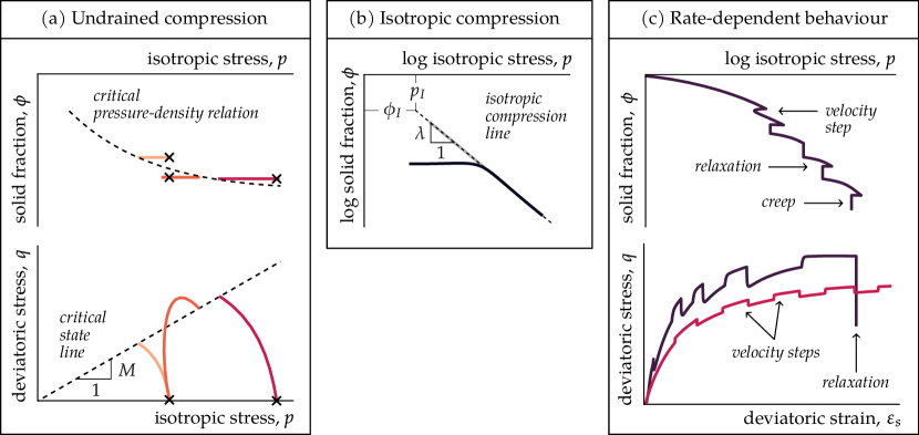
Figure 2: Schematic outline of the range of behaviours captured by the Terracotta constitutive model in its original triaxial form (re-adapted from Wiebicke & Einav, 2024). The panels showcase the model’s predictions for: (a) undrained triaxial compression, (b) isotropic compression, and (c) rate-dependent processes in uniaxial compression (top) and undrained triaxial compression (bottom).

Relative to past inelastic constitutive models for clay, and despite being strongly rooted in physics, Terracotta possesses a highly simple mathematical structure that motivates studies in geophysics. Here, we therefore seek to apply this model to direct fault shearing conditions. To this end, we present hereinafter the theoretical background behind the core of the hydrodynamic procedure and outline the Terracotta model, in its original form for triaxial testing conditions. We then tensorially generalise the model to accommodate any boundary and loading conditions. We then apply the generalised model to the specific case of direct fault shearing. The resulting equations establish a new friction law for clay-rich fault gouges, which we call Terracotta friction law in the following, as conceptualised in Figure 3.

2.1 Background setting

2.1.1 Hydrodynamics and two-stage irreversibility

In the following we summarise the main hydrodynamic principles articulated by landau2013statistical,jiang2009granular, einav2023hydrodynamics, on which Terracotta was founded upon. As such, unlike past constitutive models for clay, the development of Terracotta Wiebicke  Einav (2024) has benefitted from :

1. the conservation of energy, momentum and mass;

2. non-negativity of the entropy production;

3. scale separation of temperatures in heterogeneous media;

4. understanding of energy flow across the corresponding scales;

5. thermodynamic reciprocity Onsager (1931) of volumetric and deviatoric plastic fluxes;

6. stationarity of irreversible fluxes close to thermodynamic equilibria; and

7. the relationship between thermodynamic pressure and density.

A key feature of the model is the incorporation of the meso-temperature as a non-equilibrium state variable in clay. Unlike the conventional thermal temperature, which represents the kinetic energy of the fluctuating motions of (microscopic) atoms, the meso-temperature accounts for the kinetic energy of the fluctuating motions of (mesoscopic) clay aggregates and platelets that are overwhelmingly larger than the atoms. Through the two-stage irreversibility principle of jiang2009granular, the two temperatures are used to describe the energy flow within the material from the continuum scale down to the atomistic microscale, through the mesoscale of clay aggregates and platelets.

Following wiebicke2024simple, the state of clay materials is characterised by bulk density, $\rho$, elastic strain, $\varepsilon^{e}_{ij}$, and thermal and meso-related entropies, $s$ and $s_{m}$, which are the thermodynamic conjugates of the thermal and meso-temperatures, respectively. Accordingly, the general form of the internal energy density is defined by

$$u\equiv u\left(\rho,\varepsilon^{e}_{ij},s,s_{m}\right).$$ (1)

The complete derivation of the hydrodynamic procedure can be found in alaei2021hydrodynamic for materials that involve exactly the same set of state variables. Following the same procedure, the total stress is defined as

$$\sigma_{ij}\equiv\sigma_{ij}^{e}+\sigma^{d}_{ij}+p^{T}\delta_{ij},\qquad\sigma^{e}_{ij}\equiv\frac{\partial u}{\partial\varepsilon_{ij}^{e}},\quad p^{T}\equiv-\frac{\partial\left(u/\rho\right)}{\partial\left(1/\rho\right)}\Bigg{|}_{\varepsilon_{ij}^{e},\frac{s}{\rho},\frac{s_{m}}{\rho}},$$ (2)

where $\sigma^{e}_{ij}$ is the elastic stress tensor, $p^{T}$ is the thermodynamic pressure, and $\sigma^{d}_{ij}$ is the dissipative viscous stress, with $\delta_{ij}$ being the Kronecker delta.

Next, we determine the evolution equations for the four state variables embodied in Equation (1). Noting that throughout the article, Einstein’s summation is implied for repeated indices $i,j=1,2,3$, the evolution of the bulk density is derived from the mass balance, $\dot{\rho}+\nabla_{i}\left(\rho v_{i}\right)=0$, with $v_{i}$ being the velocity vector. We adopt the usual sign convention in soil mechanics that consider positive deformation in compression and identify the trace of the velocity gradient with the negative volumetric strain rate, $\nabla_{i}v_{i}=-\dot{\varepsilon}_{kk}\equiv-\dot{\varepsilon}_{v}$. By further introducing the solid fraction $\phi\equiv\rho/\rho_{s}$, where $\rho_{s}$ is the solid density defined as the ratio of the solid mass over the solid volume, the evolution equation for the solid fraction is defined by

$$\dot{\phi}+v_{i}\nabla_{i}\phi=\phi\dot{\varepsilon}_{v},$$ (3)

under the assumption of incompressible solid particles, i.e., $\dot{\rho}_{s}\approx 0$. The evolution for the elastic strain is given by einav2018hydrodynamic and reads

$$\dot{\varepsilon}_{ij}^{e}+v_{k}\nabla_{k}\varepsilon^{e}_{ij}+\Omega_{ik}\varepsilon^{e}_{kj}-\varepsilon^{e}_{ik}\Omega_{kj}=\dot{\varepsilon}_{ij}-\dot{\varepsilon}_{ij}^{p},$$ (4)

where $\dot{\varepsilon}_{ij}$ and $\Omega_{ij}$ are respectively the symmetric and skew-symmetric parts of the spatial velocity gradient, $\nabla_{j}v_{i}$, and $\dot{\varepsilon}_{ij}^{p}$ is the inelastic strain rate. Following scale separation Jiang  Liu (2009), where the granular entropy is replaced by the more general meso-related one Einav  Liu (2023); Wiebicke  Einav (2024), the thermal and meso-related entropies satisfy the following balance equations:

$$\dot{s}+\nabla_{i}\left(sv_{i}-f_{i}\right) =\frac{R}{T}\geq 0,$$ (5a)

$$\dot{s}_{m}+\nabla_{i}\left(s_{m}v_{i}-f^{m}_{i}\right) =\frac{R_{m}}{T_{m}},$$ (5b)

where $T\equiv\frac{\partial u}{\partial s}$ and $T_{m}\equiv\frac{\partial u}{\partial s_{m}}$ are the thermal and the meso-temperatures, respectively; $sv_{i}$ and $s_{m}v_{i}$ are the thermal and meso-related convective entropy currents; $f_{i}$ and $f^{m}_{i}$ are the thermal and meso-related dissipative entropy currents; and $R$ and $R_{m}$ are the thermal and meso-related entropy productions. Note that only the former is required to be positive-semidefinite by virtue of the second law of thermodynamics.

By combining Equations (3-5) with the momentum and energy balances, and the principle of two-stage irreversibility in the seminal work by jiang2009granular, the total rate of entropy production comprises two-scale contributions:

$$R+R_{m} \geq 0$$ (6a)

$$R_{m} =\sigma^{d}\dot{\varepsilon}_{ij}+f^{m}_{i}\nabla_{i}T_{m}-\bar{\eta}T_{m}^{2},$$ (6b)

$$R =\dot{\varepsilon}_{ij}^{p}\sigma_{ij}^{e}+f_{i}\nabla_{i}T+\bar{\eta}T_{m}^{2}\geq 0,$$ (6c)

where the viscous dissipation $\sigma^{d}\dot{\varepsilon}_{ij}$ is entirely attributed to the meso-related entropy production, unlike jiang2009granular who placed part of it in the thermal entropy. The dissipated energy within the system can either agitate the microstructure, thereby elevating the thermal temperature, $T$, or the mesostructures, thus elevating $T_{m}$, while overtime the energy can flow from the meso- to the micro-scale in a two-stage process, see Figure 1(b). The flow between the scales is given by the $\pm\bar{\eta}T_{m}^{2}$ sink/source terms, with $\bar{\eta}\geq 0$ so that the energy will indeed flow from the higher to the lower scale.

Next, we look at the dissipative fluxes in the entropy production (6), namely: $f_{i}$, $f_{i}^{m}$, $\sigma^{d}_{ij}$, and $\dot{\varepsilon}_{ij}^{p}$ and determine their hydrodynamic equations in terms of Onsager’s reciprocity relationships Onsager (1931). Following Wiebicke  Einav (2024) these are specified by

$$f_{i}=\frac{k_{T}}{T}\nabla_{i}T,\qquad f_{i}^{m}=\frac{k_{m}}{T_{m}}\nabla_{i}T_{m},\qquad\sigma^{d}_{ij}=\mathbb{X}^{d}_{ijkl}\dot{\varepsilon}_{kl},\qquad\dot{\varepsilon}^{p}_{ij}=\mathbb{X}^{p}_{ijkl}\sigma^{e}_{kl},$$ (7)

where $k_{T}$ and $k_{m}$ are the micro- and meso-scopic diffusivity coefficients, $\mathbb{X}^{p}_{ijkl}$ and $\mathbb{X}^{d}_{ijkl}$ are the transport coefficients, which could in general be functions of the state variables. Following onsager1931reciprocal, the transport coefficients must fulfil a number of reciprocity requirements stemming from time-reversal symmetry and the entropy production inequality (6), as described by wiebicke2024simple.

2.1.2 Original triaxial form of the model

Building upon the above theoretical and hydrodynamic settings, the Terracotta model Wiebicke  Einav (2024) was originally developed for standard triaxial conditions, in terms of triaxial stress and strain invariants. The isotropic stress and volumetric elastic strain invariants are defined as $p=\frac{\sigma_{ii}}{3}$ and $\varepsilon^{e}_{v}=\varepsilon^{e}_{ii}$, respectively. The deviatoric stress and elastic strain invariants read $q=(\nicefrac{{3}}{{2}}s_{ij}s_{ij})^{\nicefrac{{1}}{{2}}}$ and $\varepsilon^{e}_{s}=(\nicefrac{{2}}{{3}}e^{e}_{ij}e^{e}_{ij})^{\nicefrac{{1}}{{2}}}$, where $s_{ij}=\sigma_{ij}-p$ and $e^{e}_{ij}=\varepsilon_{ij}-\frac{\varepsilon_{v}}{3}$ are the deviatoric stress and elastic strain tensors, respectively.

The original form of the model considers isothermal processes, hence the dependency of the internal energy with respect to the thermal entropy is neglected. The internal energy density, $u$, in Equation (1), is decomposed into elastic and meso-related contributions, $u^{e}$ and $u^{m}$, through:

$$u=u^{e}(\phi,\varepsilon^{e}_{ij})+u^{m}\left(s^{m}\right),\qquad u^{e}=\phi^{6}\left(\frac{\tilde{K}}{6}{\varepsilon^{e}_{v}}^{3}+\tilde{G}\varepsilon^{e}_{v}{\varepsilon_{s}^{e}}^{2}\right),\qquad u^{m}=\frac{\Gamma}{4}{s_{m}}^{2},$$ (8)

where $\tilde{K}$ and $\tilde{G}$ represent the intrinsic bulk and shear stiffness constants, respectively; and $\Gamma=1\text{ K\textsuperscript{2}/kPa}$ is a positive constant controlling the contribution of meso-related entropy to the internal energy (its inverse could be considered as a meso-related analogue of the thermal heat capacity).

By virtue of the stress decomposition in Equation (2), the volumetric and deviatoric stress invariants are given by

$$p =p^{e}+p^{d}+p^{T},$$ (9a)

$$q =q^{e}+q^{d},$$ (9b)

where $p^{e},q^{e}$ and $p^{d},q^{d}$ are respectively the elastic and dissipative (viscous) components. The elastic volumetric and deviatoric stresses and the thermodynamic pressure are obtained from Equation (2), giving

$$p^{e} \equiv\frac{\partial u^{e}}{\partial\varepsilon^{e}_{v}}=\phi^{6}\left(\frac{\tilde{K}}{2}{\varepsilon_{v}^{e}}^{2}+\frac{3\tilde{G}}{2}{\varepsilon_{s}^{e}}^{2}\right),$$ (10a)

$$q^{e} \equiv\frac{\partial u^{e}}{\partial\varepsilon^{e}_{s}}=3\tilde{G}\phi^{6}\varepsilon_{v}^{e}\varepsilon_{s}^{e},$$ (10b)

$$p^{T} =\frac{T_{m}^{2}}{\Gamma}\Leftarrow T_{m}=\frac{\Gamma}{2}s^{m},$$ (10c)

where the elastic contribution in the thermodynamic pressure, i.e., $5u^{e}$, was found negligible Wiebicke  Einav (2024) and is thus omitted for the sake of simplicity. The above equations are completed by the constitutive relationships for the dissipative fluxes, $p^{d}$ and $q^{d}$, and the evolution equations for the solid fraction, Equation (3), the meso-temperature, $T_{m}$, and the elastic strain, $\varepsilon_{v}^{e}$ and $\varepsilon_{s}^{e}$. Their derivation follows the hydrodynamic procedure, cf. subsection 2.1.1, and the exact procedure is sketched below for the generalised model in tensorial form. For the original derivation in triaxial conditions, we refer to wiebicke2024simple, with the corresponding expressions presented in Figure 3(a).

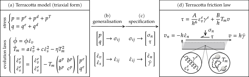
Figure 3: Summary of the mathematical development from (a) the original Terracotta model for triaxial conditions to its (b) tensorial generalisation to its (c) specification for direct fault shearing conditions, which finally reduces to (d) the resulted Terracotta friction law. The total stress in Terracotta is equal to the sum of elastic, thermodynamic, and viscous contributions. The elastic stress (in invariant form $p^{e}$ and $q^{e}$), is expressed by Equation (10a); the thermodynamic pressure ($\smash{p^{T}}$) is defined according to (2); while the viscous stress (in invariant form $\smash{p^{d}}$ and $\smash{q^{d}}$) is expressed by Equation (11); and finally, the plastic transport coefficients are given by Equation (12). The resulting friction law for considers the slip velocity $v$, gouge thickness $h$, meso-temperature $T_{m}$, and elastic strains $\gamma^{e}$ and $\varepsilon_{v}^{e}$.

More precisely, the calibration of the triaxial invariants of the viscous stress, $p^{d}$ and $q^{d}$, is performed in the simplest way to ensure the semi-positivity of the viscous dissipation, leading to the following formulation:

$$p^{d}=aT_{m}\dot{\varepsilon}_{v},\quad q^{d}=cT_{m}\dot{\varepsilon}_{s},$$ (11)

where the viscous stress is made to decay to zero as the meso-temperature approaches thermodynamic equilibrium ($T_{m}\rightarrow 0$), as expected from non-equilibrium thermodynamic properties.

Next, the stationary value of the meso-temperature is used to calibrate the dependence of the plastic transport coefficients, so to enable the recovery of experimental critical state observations. This calibration approach was proposed by wiebicke2024simple and was informed by two canonical asymptotic states: normal consolidation state emerging by continuous isotropic compression and the critical state emerging by continuous shearing Wiebicke  Einav (2024). Following this procedure, the following plastic transport coefficients were obtained:

$$a^{p}=\sqrt{\frac{\eta}{a}}\frac{1}{p_{c}(\phi)}\quad b^{p}=-a\frac{q^{e}}{M^{2}p^{e}},\quad c^{p}=\sqrt{\frac{\eta}{c}}\frac{1}{M\omega p_{c}(\phi)}+\frac{a}{M^{2}},\quad p_{c}(\phi)=p_{I}\phi^{\lambda},$$ (12)

where $a$, $c$ are positive material constants, $\omega$ and $M$ are the parameters describing the critical state line <see Figure 2 and refer to¿wiebicke2024simple, and $p_{c}(\phi)$ describes the stress-density relationship on the isotropic compression line, where $\lambda$ is the slope of the isotropic compression line on a bi-logarithmic plot of pressure against solid fraction and $p_{I}=\phi_{I}^{-\lambda}$ (kPa) is calibrated with $\phi_{I}$ representing the solid fraction at a reference pressure of $1$ kPa, see Figure 2.

2.2 Generalisation to the tensorial form

Based on the hydrodynamic procedure, we extend the above form of the Terracotta model to its tensorial form with the objective of addressing more general loading conditions than just triaxial loading, including those related to the shearing of fault gouges. By following the specification of the internal energy density given in Equation (8), we generalise the elastic contribution in terms of the full elastic strain tensor, $\varepsilon_{ij}^{e}$, namely

$$u^{e}=\phi^{6}\left(\frac{\tilde{K}}{6}{\varepsilon^{e}_{v}}^{3}+\tilde{G}\varepsilon^{e}_{v}e^{e}_{ij}e^{e}_{ij}\right),$$ (13)

which is equivalent to the original expression in Equation (8) when specified in terms of triaxial invariants. As in the triaxial form of Terracotta, we neglect the dependence of the internal energy on the thermal temperature. However, such dependencies could easily be accounted for through the hydrodynamic procedure, as further discussed in paragraph 2.2.1.

By virtue of Equation (2), the elastic stress tensor becomes

$$\sigma^{e}_{ij}\equiv\frac{\partial u}{\partial\varepsilon_{ij}^{e}}=\phi^{6}\Bigg{(}\frac{\tilde{K}}{2}\varepsilon^{e^{2}}_{v}\delta_{ij}+\tilde{G}\delta_{ij}e^{e}_{kl}e^{e}_{kl}+2\tilde{G}\varepsilon^{e}_{v}e^{e}_{ij}\Bigg{)},$$ (14)

whose volumetric and deviatoric invariants are exactly the same as those in the triaxial formulation, i.e., Equations (10). The mesoscopic component of the internal energy, $u^{m}$, is kept the same as in Equation (8), ensuring that the resulting thermodynamic pressure in Equation (10c), $p^{T}$, also remains unchanged.

2.2.1 Thermal and meso-related heat equations

The concept of two-stage irreversibility Jiang  Liu (2009) provides us with the form of the evolution equations for the micro- and meso-temperatures. The full hydrodynamic derivation of their corresponding rate equations can be found in [Appendix A]riley2023constitutive, considering the two-stage irreversibility. In the absence of convective entropy currents, the evolution equations for the micro- and meso-temperatures are given by

$$\dot{T} =\frac{k_{T}}{c_{T}\rho}\nabla^{2}_{i}T+\dot{\varepsilon}_{ij}^{p}\sigma^{e}_{ij}+\bar{\eta}T_{m}^{2}$$ (15a)

$$\frac{2T_{m}}{\Gamma}\dot{T}_{m} =k_{m}\nabla^{2}_{i}T_{m}+\sigma^{d}_{ij}\dot{\varepsilon}_{ij}-\bar{\eta}T_{m}^{2},$$ (15b)

where $c_{T}$ is the micro-related specific thermal heat capacity. Note that the Laplace operator, $\nabla^{2}_{i}\cdot$, can physically capture second-gradient phenomena, known as non-local effects in granular physics Kamrin  Koval (2012); Henann  Kamrin (2013). Predicting these phenomena requires spatial integration of the underlying boundary value problem, which is beyond the focus of the current paper. From here on, we shall therefore neglect the second gradient terms and focus on phenomena that happen homogeneously within representative elementary volumes, independent of non-local effects.

2.2.2 Dissipative fluxes and calibration

By virtue of the time-reversal symmetry requirements, the relationships for the viscous stress and plastic strain rate introduced in Equation (7) are generalised in term of the volumetric invariant and the deviatoric tensor as follows,

$$\begin{bmatrix}p^{d}\\ s^{d}_{ij}\end{bmatrix}=\frac{2T^{m}}{\Gamma}\begin{pmatrix}a^{d}&b^{d}_{kl}\\ b^{d}_{ij}&c^{d}_{ijkl}\end{pmatrix}\begin{bmatrix}\dot{\varepsilon}_{v}\\ \dot{e}_{kl}\end{bmatrix},\qquad\begin{bmatrix}\dot{\varepsilon}_{v}^{p}\\ \dot{e}^{p}_{ij}\end{bmatrix}=T_{m}\begin{pmatrix}a^{p}&b^{p}_{kl}\\ b^{p}_{ij}&c^{p}_{ijkl}\end{pmatrix}\begin{bmatrix}p^{e}\\ s^{e}_{kl}\end{bmatrix}.$$ (16)

Next, following wiebicke2024simple, we consider the energy sink coefficient to be linearly proportional to the meso-temperature, i.e., $\bar{\eta}=2\frac{\eta}{\Gamma}T_{m}$. We then substitute the constitutive relationship for the viscous stress in the meso-related heat equation (15b), so by neglecting non-local effects we obtain the following evolution equation for the meso-temperature

$$\dot{T}_{m}={a}\dot{\varepsilon}_{v}^{2}+{c}\dot{e}_{ij}\dot{e}_{ij}-\eta T_{m}^{2},$$ (17)

where in order to retrieve the expression given in [Equation 36]wiebicke2024simple, we use

$$a^{d}={a},\quad\quad b^{d}_{ij}\equiv 0_{ij},\quad\quad c^{d}_{ijkl}\equiv\frac{2}{3}{c}\delta_{ik}\delta_{jl},$$ (18)

where $a$ and $c$ are positive material constants.

Using the above expressions and following Wiebicke and Einav’s calibration procedure, we obtain the following plastic transport coefficients for the tensorially general case:

$$a^{p}=\sqrt{\frac{\eta}{a}}\frac{1}{p_{c}(\phi)},\quad b_{ij}^{p}=-\frac{3}{2}\frac{a^{p}}{M^{2}}\frac{s^{e}_{ij}}{p^{e}},\quad c_{ijkl}^{p}=\frac{3}{2}\left(\sqrt{\frac{\eta}{c}}\frac{1}{M\omega p_{c}(\phi)}+\frac{a^{p}}{M^{2}}\right)\delta_{ik}\delta_{jl}.$$ (19)

Given the specific form of the transport coefficients, the full tensorial expressions for the viscous stress and the plastic strain rate become

$$\sigma^{d}_{ij} =\frac{2T^{m}}{\Gamma}\left({a}\dot{\varepsilon}_{v}\delta_{ij}+\frac{2}{3}{c}\dot{e}_{ij}\right),$$ (20a)

$$\dot{\varepsilon}^{p}_{ij} =\frac{T^{m}}{M^{2}p_{1}\phi^{\lambda}}\sqrt{\frac{\eta}{a}}\left[\left(M^{2}-\left(\frac{q^{e}}{p^{e}}\right)^{2}\right)\frac{p^{e}}{3}\delta_{ij}+\frac{3}{2}\sqrt{\frac{{a}}{{c}}}\frac{M}{\omega}s^{e}_{ij}\right].$$ (20b)

It is worth noticing that when evaluated in terms of the volumetric and deviatoric invariants – namely, $p^{d},q^{d}$ and $\dot{\varepsilon}^{p}_{v},\dot{\varepsilon}^{p}_{s}$ – the above expressions yield the exact same form of the transport coefficients as those derived in the original triaxial formulation of Terracotta model. Moreover, note that the requirement for the semipositive definiteness of the plastic transport coefficients coincides with that identified in [Equation (53)]wiebicke2024simple.

2.3 Specification of the Terracotta friction law

From the newly expressed tensorial form of the Terracotta model, we specify the boundary conditions of an isolated fault gouge and derive the corresponding friction law under direct shearing configuration. In so doing, we use plane strain conditions and adopt the following minimal Voigt notation:

$$\sigma_{ij}\rightarrow\begin{bmatrix}\sigma_{n}\\ \sigma_{\ell}\\ \tau\end{bmatrix},\qquad\varepsilon^{e}_{ij}\rightarrow\begin{bmatrix}\varepsilon^{e}_{n}\\ \varepsilon^{e}_{\ell}\\ \gamma^{e}\end{bmatrix},$$

with superscripts $n,\ell$ referring to the normal and longitudinal directions, respectively. The equivalence with the tensorial form is given by $\sigma_{n}=\sigma_{11}$, $\sigma_{\ell}=\sigma_{22}=\sigma_{33}$, $\tau=\sigma_{12}$ and $\varepsilon^{e}_{n}=\varepsilon^{e}_{11}$, $\varepsilon^{e}_{\ell}=\varepsilon^{e}_{22}=\varepsilon^{e}_{33}$, $\gamma^{e}=2\varepsilon^{e}_{12}$.

Next, we consider a fault gouge of constant length $L$ and variable thickness $h$, whose state is determined by the following initial conditions at thermodynamic equilibrium

$$h(0)=h^{0},\quad\phi(0)=\phi^{0},\quad T_{m}(0)=0,\quad\varepsilon^{e}_{ij}(0)=\begin{bmatrix}\varepsilon^{e^{0}}_{n}\\ \varepsilon^{e^{0}}_{\ell}\\ 0\end{bmatrix},\quad\sigma_{ij}(0)=\begin{bmatrix}\sigma^{e^{0}}_{n}\\ \sigma^{e^{0}}_{\ell}\\ 0\end{bmatrix},$$ (21)

where the initial conditions for the elastic strain are obtained by equating the elastic stress in Equation (14) with the prescribed values for $\sigma^{e}_{n},\sigma_{\ell}^{e}$, under either isotropic or uniaxial stationary compression.

Starting from the initial state in Equation (21), the fault gouge is subjected to a slip velocity $v$, see Figure 3(d). To ensure a constant normal stress $\sigma_{n}=\sigma_{n}^{0}$, the material undergoes dilation or contraction along the normal direction, following the evolution of the gouge thickness $h$ and its compaction velocity, $v_{n}$, again see Figure 3(d). With that, the resulting Terracotta friction law reads

(22)

where the constants $A\equiv\tilde{G}\left(\phi^{0}h^{0}\right)^{6}$ and $B\equiv(2/3)c/\Gamma$. The above equation is boxed in order to highlight it as the main result of the paper, which is formulated in terms of the following evolution equations for the state variables

$$\dot{\varepsilon}_{v}^{e} =\dot{\varepsilon}_{n}-\frac{T_{m}p^{e}}{p_{c}(\phi)}\sqrt{\frac{\eta}{a}}\left(1-\left(\frac{q^{e}}{Mp^{e}}\right)^{2}\right),$$ (23a)

$$\dot{\gamma}^{e} =\dot{\gamma}-\frac{3T_{m}\tau^{e}}{M\omega p_{c}(\phi)}\sqrt{\frac{\eta}{c}},$$ (23b)

$$\dot{T}_{m} =\left(a+\frac{4c}{9}\right)\dot{\varepsilon}_{n}^{2}+\frac{c}{3}\dot{\gamma}^{2}-\eta T_{m}^{2},$$ (23c)

$$\dot{h} =-h\dot{\varepsilon}_{n},$$ (23d)

where $\phi=(\phi^{0}h^{0})/h$. The total strain rates are then given in terms of the normal and slip velocities that act as the rate variables in the present model:

$$\dot{\gamma} =\frac{v}{h}\;\text{ such that }v=v(t),$$ (24a)

$$\dot{\varepsilon}_{n} =-\frac{v_{n}}{h}\;\text{ such that }\dot{\sigma}_{n}\left(\text{state},v,v_{n}\right)=0,$$ (24b)

where $v(t)$ is imposed as function of time. Appendix A: Numerical implementation presents further details of the numerical implementation of the friction law <cf.¿github.

In the following, the shear stress evolution predicted by the Terracotta friction law is expressed in terms of the friction coefficient, i.e., $\mu=\tau/\sigma_{n}$.

2.3.1 Calibration of material parameters

The Terracotta friction law (Equations 22-24) requires the specification of nine material parameters ($\tilde{K}$, $\tilde{G}$, $M$, $\omega$, $\lambda$, $\phi_{I}$, $a$, $c$, and $\eta$). However, when compared to conventional rate-and-state friction laws, which in their simplest form involve four to five parameters, the calibration of these parameters follows relatively simple and standard tests Wiebicke  Einav (2024) and account for much broader physics. For example, the two elastic constants, $\tilde{K}$ and $\tilde{G}$, allow us to describe pressure and density dependent elastic responses and can be calibrated using conventional elastic wave measurements <cf.¿riley2023consistent or by fitting the model to observed stress-strain responses, as performed hereafter. Parameters $\phi_{I}$ and $\lambda$, which define inelastic compressibility that also goes beyond conventional both rate-and-state and micromechanically-inspired friction laws, can be directly calibrated from isotropic/uniaxial compression tests or inferred from the post-peak slope in triaxial compression or direct shear tests. The two critical state parameters, $M$ and $\omega$, can be obtained from triaxial compression or direct shear tests, with $\omega=0.5$ being a good value in the absence of density measurements, in agreement with the tacit assumption for clay in the modified cam clay model Wood (1990) of soil mechanics. The remaining three rheological parameters, $\eta$, $a$, and $c$, require calibration thorough rate-dependent experiments such as velocity stepping or slide-hold-slide tests, as those considered below.

2.3.2 Calibration of system parameters

Together with the above material parameters, it is necessary to determine appropriate initial conditions for the normal stress, $\sigma_{n}^{0}$, solid fraction, $\phi^{0}$, and layer thickness, $h^{0}$. The normal stress is conventionally prescribed or measured in laboratory experiments <cf.¿saffer2003comparison, or in the field may be estimated as the overburden stress from the fault gouge depth <cf.¿kanamori2004physics. The solid fraction in general varies through the thickness of the fault gouge <see¿https://doi.org/10.1029/2022JB025666, though as discussed earlier all such gradients are neglected in the present analysis. One way to determine the initial layer thickness is to follow rice2006, who associated it with the localised shear zone within the gouge of less than $1\div 5$ mm. This shear zone of an ultra-cataclastic gouge is influenced by factors such as fault maturity and the chemical composition of its materials.

In clay, on which the current paper focuses, the thickness of the localised shear zones in the fault gouge is considered to be approximately $10\div 100$ times the clay platelet diameter, which is of the order of $1$ µm Morgenstern  Tchalenko (1967); Rice (2006); Haines . (2013); Bigaroni . (2023); Volpe . (2024). Although studies have explored the effects of earthquake nucleation and seismic events on the layer thickness using both laboratory samples and natural fault gouges <e.g.,¿[among others]byerlee1976note,93JB03361,2011JB008264,evans1990thickness,JB095iB05p07007,scuderi2014physicochemical,lyu2019mechanics,bedford2021role, the quantification of this relationship remains elusive. Therefore, the impact of layer thickness on the nucleation and seismicity is carefully analysed in Section 4.

3   Terracotta friction law: performance and validation

The purpose of the current section is to demonstrate the capabilities of the proposed Terracotta friction law in capturing the complex rate- and state-dependent frictional behaviour of clay-rich fault gouges. To this end, the analysis will make use of a variety of experiments on clay gouges conducted by saffer2003comparison, bedford2022fault, and ashman2023effect, which explore the shear response of gouge media under different normal stress values and controlled velocity steps, as well as the evolution of the gouge’s thickness $h$.

As a start, we determine the corresponding material and system parameters of the Terracotta friction law. In particular, an initial guess is made based on previous values obtained by wiebicke2024simple, which are then iteratively updated to fit the experimental curves, as specified below for each series of tests. The initial conditions are set according to the available experimental values of the normal stress, $\sigma_{n}^{0}$, and gouge’s thickness, $h^{0}$. In the absence of information regarding the thickness of potential shear band, the gouge thickness, $h^{0}$ is assumed to match the initial thickness of the tested samples. While selecting a smaller value for $h^{0}$ would result in higher shear strain rates and alter the rheological parameters, the conceptual conclusions should remain valid for the scenarios considered here. Furthermore, since in the relevant papers information was not available concerning the initial values of the solid fraction $\phi^{0}$, the following analysis will consider it as a fitting parameter against the experimental results. Finally, the elastic strain state is initialised by isotropically compressing the simulated sample from a reference stress-free configuration, see Equation (21). Table 1 presents the model parameters and initial conditions for the gouge materials considered hereinafter.

Mechanical parameters Rheological parameters $\tilde{K}$ $\tilde{G}$ $M$ $\omega$ $\lambda$ $\phi_{I}$ $a$ $c$ $\eta$ Gouge (MPa) (MPa) (-) (-) (-) (-) (Ks) (Ks) (K^-1s^-1) Illite 1040 400 0.96 0.6 10 0.20 7 7 7.2$\cdot$10⁴ Smectite 260 100 0.42 0.5 10 0.28 2.4$\cdot$10⁴ 2.4$\cdot$10⁴ 10 Kaolinite 15.6 12.5 0.44 0.4 4.5 0.05 0.42 10 3$\cdot$10⁶

Table 1: Parameters for the Terracotta friction law calibrated for the experiments conducted by Saffer & Marone (2003) and Bedford et al. (2022) for illite shale, smectite, and kaolinite.

3.1 Experiments from Saffer and Marone (2003)

The tests conducted by saffer2003comparison consist of shearing of synthetic and natural gouges, in a double-direct shear geometry, at room humidity and temperature. Specimens were subjected to different levels of constant normal stress and sheared with varying velocities ranging from 1 to 200 $\mu$m/s. Focusing on clay-rich gouges, here we only study the tests on illite shale and smectite. The gouge layers were prepared by applying an initial compaction to the original sample resulting in an initial thickness $h^{0}$ equal to $2.25$ and $2.75$ mm for smectite and illite shale, respectively. Next, the gouge was sheared with frequent velocity stepping.

The initial conditions for the Terracotta friction law consider the effective normal stress prescribed in the experiments, i.e. $\sigma_{n}=20$ MPa, the aforementioned values for $h^{0}$, while the solid fractions were chosen as $\phi^{0}=0.57,0.71$ for the illite and smectite gouges, respectively.

Figure 4 displays the frictional behaviour during the experiments and the Terracotta friction law given the parameters in Table 1 for the corresponding smectite and illite shale tests. Both the experiments and the predictions are characterised by an initially rapid increase in the friction coefficient during the loading phase, before peak friction coefficient at around $\gamma\approx 0.5\div 1$. Post-peak the friction coefficient gradually decays towards a plateau, whose value depends on the gouge’s material, exemplified by the critical state constant, $M$, and the shear velocity.

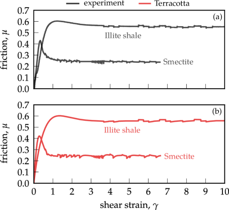
Figure 4: Shear response of illite shale and smectite gouges under constant normal stress $\sigma_{n}=20$ MPa, shown in terms of the friction coefficient, $\mu=\tau/\sigma_{n}$, versus the shear strain, $\gamma$: (a) experiments (Saffer & Marone, 2003), and (b) model’s predictions.

The Terracotta friction law shows a strong capacity in replicating the responses of both specimens, including not only the under velocity stepping during mature shearing, but the peak and pre-peak values of the friction coefficient. In particular, despite the very rich and variegate velocity dependence of the friction coefficient observed in the experiments, the new friction law is able to predict and distinguish between the large and limited velocity strengthening behaviour displayed by illite and smectite, respectively. The ability of the new law to adequately represent both pre- and post-peak behaviours moves beyond previously proposed rate-and-state and micromechanically-inspired frictional laws, where the elasticity of the gouge is ignored.

Note the presence of some minor differences between the experiments and the simulations in the amplitude of the jumps of the friction coefficient. While the experiments display a predominantly symmetrical trend of the friction coefficient with respect to up- and down-steps of the slip velocity, $v$, the predictions show jumps of $\mu$ more pronounced along one direction (up-steps for illite, and down-steps for smectite). The reason lies on the evolution of the meso-temperature, with a quadratic decay to the steady-state value, cf. Equation (17). Nevertheless, the predictions are found to be in good agreement with the experiments for the entire range of variation of the shear strain, in spite of the complex loading scenarios and the idealised boundary conditions (cf. direct shear).

It is also worth noticing that Terracotta enables the prediction of diverse rate-dependent responses <cf.¿wiebicke2024simple. In particular, the Terracotta friction law predicts the characteristic behaviour displayed by illite with rapid transitions of the stress between constant plateaus, at varying of the shear rate, often referred to as ‘isotach’ behaviour Šuklje (1969) in soil mechanics, but also the instantaneous jumps of the shear stress followed by a relaxation towards a new residual rate-dependent plateau as shown by smectite. Those rate-dependent phenomena are governed by one of the new ingredient introduced in Terracotta, the meso-temperature. This is in contrast with classical rate-and-state frictional laws Dieterich (1979, 1981); Ruina (1983) where the form of the rate-dependence is described in terms of (fixed) parameters ($a$ and $b$). Here, the meso-temperature and, more precisely, the speed at which it approaches a new steady state following its evolution Equation (17), influences the range of predicted rate-dependent behaviours <for further details, we refer to¿wiebicke2024simple.

3.2 Experiments from Bedford et al. (2022)

bedford2022fault performed experiments on fault gouge materials within a triaxial deformation apparatus in a direct-shear arrangement, involving both fully homogeneous and laterally heterogeneous gouges of kaolinite, quartz, and mixtures of them. The gouges, with an initial thickness $h^{0}\approx 1$ mm, were subjected under a constant (effective) normal stress $\sigma_{n}=40$ MPa and sheared under relatively slow velocities between $0.3\leq v\leq 3$ µm/s.

Here, we only focus on the clay-rich experiment that involved kaolinite, as presented in Figure 5. The initial thickness and normal stress are set to match the experimental values, while the initial solid fraction is chosen as $\phi^{0}=0.65$. This corresponds to an overconsolidation ratio of $p_{c}/p=1$, where $p=\sigma_{n}$ at the initial state.

As for the previous tests, the evolution of the friction coefficient during the slip was provided, as well as the evolution of the gouge thickness. The latter was tracked by measuring the volume of fluid expelled from the sample by means of servo-control pumps, which revealed a substantial amount of consolidation. In particular, the inference of the thickness was made while assuming constant sliding area, such that the volumetric straining was approximated through changes only to the layer thickness without orthogonal straining. Importantly, the data of the thickness variations allows us to corroborate the volumetric nature of the Terracotta friction law.

The new friction law is calibrated based on the time evolution of the gouge thickness, $h$, presented in Figure 5(b), before the application of velocity steps that initiates after slip displacement of $1.5$ mm. The comparison of the model against the experimentally measured friction coefficient, gouge thickness, and normal velocity, $v_{n}$, is presented in Figure 5. Despite an underestimation of the peak value of the friction coefficient, the predictions beyond this peak are found to be in good agreement with the experimental results, and demonstrate capacity to capture the isotach phenomenon Šuklje (1969) at both up- and down-steps of the velocity. The evolution of the gouge thickness is well captured as well, thanks to the adopted calibration procedure. In particular, the model agrees with the experiments until the first downstep of the velocity, around $2$ mm slip, where the friction law predicts a near constant sample thickness, in contrast with the slight continual compaction observed in the experiments. It is worth noticing that the intrinsic volumetric nature of the new friction law depends on the time evolution of two rates – slip velocity $v(t)$ as well as compaction velocity $v_{n}(t)$. To this purpose, we also inferred the experimental evolution of $v_{n}$, by means of a first-order finite difference scheme from the test data of the thickness, i.e., $v_{n}(t)\approx v(t)\Delta h/\Delta d$, where $\Delta h$ and $\Delta d$ are the increments of the gouge’s thickness and slip displacement. As shown in the corresponding Figure 5(c), the predicted normal rate, $v_{n}$, well matches the experiments. Despite some minor differences mostly due to the resolution of the recorded evolution of the thickness, the Terracotta friction law correctly predicts the values of the compaction velocity before and during velocity stepping, with minor underestimation of the repeated upsteps of the shear velocity.

Finally, it is worth noticing that the minor differences between the predictions and the experiment may be due to the working assumption of material homogeneity in the current initial development. A further reason may be due to the idealised boundary conditions considered in the specification of the new friction law (see subsection 2.3) as compared to the actual setup of the present experiment Bedford . (2022), where soft silicone spacers were positioned at end of the gouge layers in order to accommodate longitudinal displacements without supporting any load.

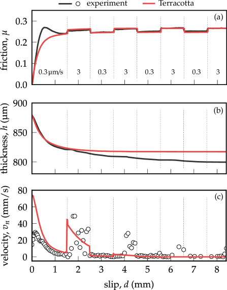
Figure 5: Comparison between experiments (Bedford et al. 2022) and the Terracotta friction law for kaolinite at normal stress $\sigma_{n}=40$ MPa. Evolution of (a) friction coefficient, $\mu$, (b) gouge thickness, $h$, and (c) normal velocity, $v_{n}$.

3.3 Experiments from Ashman and Faulkner (2023)

The experiments performed by ashman2023effect use the same experimental setup of bedford2022fault, again on kaolinite gouges in order to study their frictional behaviour under velocity steps. However, in their study they additionally inspected the influence of the normal stress, $\sigma_{n}$. Accordingly, we consider the exact same material and rheological parameters obtained from the calibration of the previous test, as listed in Table 1, and vary the initial solid fraction to keep a constant overconsolidation ratio of $p_{c}/p=1$.

Figure 6 compares the predictions provided by the Terracotta friction law against the experimental results. An overall good agreement is found, which is notable considering that no adjustment of the material parameters was made for the different normal stresses. In particular, the decreasing amplitude of the isotachs at increasing normal stress is accurately predicted by the new friction law, with only minor differences visible under the least stressed configuration, i.e., $\sigma_{n}=10$ MPa.

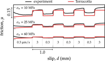
Figure 6: The variations in the friction coefficient, $\mu$, of kaolinite in response to seven slip velocity steps under different constant normal stresses of $\sigma_{n}=10,25,60$ MPa, in terms of experiments (Ashman & Faulkner, 2023), and the Terracotta friction law. The friction coefficient curves are plotted at the same scale, around a mean value of $\mu=0.33$, with an offset of 0.15 along the y-axis for clarity.

4   Terracotta-spring model for earthquakes dynamics

This section extends the analysis to investigate the predictive capabilities of the Terracotta friction law in modelling earthquake nucleation, stick-slip instabilities, and their occurrence. We focus attention on exploring the influence of the physical parameters that are unique to this new friction law, such as slip thickness, meso-temperature, and solid fraction, and which cannot be effectively examined using conventional rate-and-state models Kanamori  Brodsky (2004); Dieterich (1979, 1981); Ruina (1983); Pipping (2019). To this end, we connect the Terracotta friction law to a spring-dashpot representation of the host rock, as shown in Figure 1(c). We then use this combined Terracotta-spring model to analyse the statistical dynamics of earthquakes and its energetical terms. In this model the mass, $m$, represents a mobilised mass sliding over a frictional gouge layer of thickness $h$ and length $L$, undergoing a slip displacement $d$ due to the far-field movement of the tectonic plates, which is prescribed by the slip velocity $v_{\infty}$. The mass is connected to a spring with stiffness $k={G}_{*}L$, which represents the effective mobilised stiffness of the host rock, where ${G}_{*}$ is the corresponding shear modulus. This spring is connected in parallel to a dashpot with damping coefficient $\varsigma$, equivalent to the apparent viscosity of the host rock. Subjected to an effective overburden normal stress $\sigma_{n}$, the frictional shear layer develops a shear stress $\tau$, governed by the evolution of Terracotta’s state variables and the slip velocity, $v=\dot{d}$, see subsection 2.3.

4.1 Governing equations

Using force balance, the motion of the Terracotta-spring model is described as follows

$$m\dot{v}=k(d_{\infty}-d)+\varsigma(v_{\infty}-v)-S\tau,$$ (25)

where $m=\rho_{*}L^{3}$ is the mobilised mass assuming a cuboid of length $L$, $S=L^{2}$ is the contact area, $d_{\infty}=v_{\infty}t$ is the displacement at the extremity of the spring-dashpot configuration, and $\varsigma=2\zeta\omega_{n}m$, where $\zeta$ is the damping ratio and $\omega_{n}=\sqrt{\nicefrac{{{G}_{*}}}{{\rho_{*}}}}/L$ is the natural frequency of the system, assuming an equivalent linearly elastic isotropic medium for the host rock, while $\rho_{*}$ is its bulk density.

Next, we introduce the following dimensionless variables

$$\hat{t} =\frac{t}{\mathscr{T}},\quad\gamma=\frac{d}{D},\quad\gamma_{\infty}=\frac{d_{\infty}}{D},\quad\varepsilon_{n}=1-\frac{h}{D},$$ (26a)

$$\gamma^{\prime} =\frac{v}{v_{\infty}},\quad\varepsilon_{n}^{\prime}=-\frac{v_{n}}{v_{\infty}},\quad\theta=\frac{T_{m}}{\Theta},$$ (26b)

where $D$, $\mathscr{T}$, and $\Theta$ are respectively the characteristic length, time, and meso-temperature, i.e.,

$$D=h^{0},\quad\mathscr{T}=\frac{D}{v_{\infty}},\quad\Theta=\frac{1}{\mathscr{T}}\sqrt{\frac{c}{3\eta}}.$$ (27)

Here, $D$ coincides with the initial value of the fault gouge thickness, $\mathscr{T}$ denotes the timescale over which shear strain accumulates within the gouge, and $\Theta$ corresponds to the ambient meso-temperature – that is, the steady-state value reached under a constant slip velocity $\mathscr{T}^{-1}$ and constant dilation/contraction of the fault gouge. Accordingly, the non-dimensional forms of Equations (25) and (22) read

$$\gamma^{\prime\prime} =\hat{k}\left(\gamma_{\infty}-\gamma\right)+\hat{\varsigma}\left(1-\gamma^{\prime}\right)-\hat{N}\mu,\vspace{10pt}$$ (28a)

$$\mu =\frac{\hat{A}}{\left(1-\varepsilon_{n}\right)^{6}}\varepsilon_{v}^{e}\gamma^{e}+\frac{\hat{B}}{1-\varepsilon_{n}}\theta\gamma^{\prime},$$ (28b)

with

$$\begin{split}\hat{k}&=\frac{\epsilon^{2}}{\mathscr{C}},\quad\hat{\varsigma}=2\zeta\sqrt{\hat{k}},\quad\hat{N}=\frac{\hat{k}}{\epsilon\kappa},\\ \hat{A}&={\phi^{\vspace{-4pt}0}}^{6}\frac{\tilde{G}}{\sigma_{n}},\quad\hat{B}=\mathscr{T}^{-1}\Theta\frac{2c}{3\Gamma\sigma_{n}},\\ \epsilon&=\frac{D}{L},\quad\mathscr{C}=\frac{\rho_{*}v_{\infty}^{2}}{{G}_{*}},\quad\kappa=\frac{G_{*}}{\sigma_{n}},\end{split}$$ (29)

where $\mathscr{C}$ is the Cauchy number representing the ratio of inertial and elastic forces through the host rock and $\epsilon$ is the thickness-to-length ratio of the fault gouge.

The dynamics of the Terracotta-spring model is governed by six non-dimensional variables – $\gamma$, $\varepsilon_{n}$, $\gamma^{\prime}$, $\varepsilon_{n}^{\prime}$, $\varepsilon^{e}_{v}$, $\gamma^{e},$ and $\theta$ – in terms of the non-dimensional time $\hat{t}$. The model’s behaviour is determined through the time integration of Equation (28), along with the evolution equations for the state variables $\varepsilon^{e}_{v}$, $\gamma^{e}$, $\theta$, and $\delta_{n}$, as presented in Equation (23). We recall that the evolution of the normal displacement, $\delta_{n}$, is prescribed by ensuring a constant stress $\sigma_{n}$. The initial conditions for these state variables are given in Equation (21).

5   Terracotta-spring model: results

The previous section has described the attachment of the Terracotta friction law with a spring-dashpot system representative of the host rock. Here we analyse the corresponding performance for modelling earthquake dynamics. Besides the material constants associated with the friction law in subsection 2.3 and the initial conditions ($\sigma_{n}$, $h^{0}$, and $\phi^{0}$), five additional non-dimensional parameters of the spring-slider system must be specified: $\mathscr{T}$, $\epsilon$, $\mathscr{C}$, $\kappa$, and $\zeta$. Their values depend on the actual configuration of the fault gouge, either in laboratory experiments or in the field. To this end, in the following a parametric analysis is performed, as motivated by previous such explorations of rate-and-state friction laws Rice (1985); Rudnicki (1988); Marone . (1990); Rice  Ruina (1983); Y. Gu  Wong (1991).

Here, we consider a clay-rich gouge whose material parameters are similar to those obtained for the validation against laboratory tests in Section 3, as well as against triaxial experiments in wiebicke2024simple. The material and in-situ dimensional properties are given in Table 2, where the volumetric and deviatoric rheological constants are assumed equal, i.e., $a\equiv c$. The following analysis is presented in terms of a unit fault gouge segment, $L=1$ m, and constant stiffness to focus attention on the new and key ingredients of the Terracotta-spring model. In most scenarios, the results are being presented in their non-dimensional form to further enable scaling of the relationships identified in this work. Nonlinear stability analyses of the present model are expected to gather additional insights in the occurrence and magnitude of the predicted stick-slip instabilities <cf.¿riceruina83,gu1984slip, gu1991,ciardo2024non, but such investigation remains beyond the scope of the present work.

Material parameters In-situ properties $\tilde{K}$ $\tilde{G}$ $M$ $\omega$ $\lambda$ $\phi_{I}$ $c$ $\eta$ $G_{*}$ $\rho_{*}$ $\zeta$ $v_{\infty}$ (GPa) (GPa) (-) (-) (-) (-) (Ks) (K^-1s^-1) (GPa) (kg/m³) (-) (µm/s) 18.2 7 0.9 0.6 10 0.225 $10^{5}$ $0.01$ 10 2500 $0\div 1$ $10^{-5}\div 50$

Initial conditions $\sigma_{n}$ $\phi^{0}$ $h^{0}$ (MPa) (-) (mm) $\;5\div 640\;$ $\;0.52\div 0.9\;$ $\;0.001\div 10\;$

Table 2: Baseline parameters for the Terracotta-spring model per metre unit length of a fault gouge segment. The rheological parameters are assumed to be equal, i.e., $a\equiv c$. The far-field tectonic velocity, $v_{\infty}$, varies between $1$ mm/year ($\sim 3\cdot 10^{-5}$ µm/s) and $50$ µm/s.

5.1 Benchmark

To demonstrate the predictive capabilities of the Terracotta-spring model, we consider a benchmark scenario where the parameters are set as follows: $v_{\infty}=1$ cm/year (equivalent to $\sim 3\cdot 10^{-4}$ µm/s), $\zeta=0$ (undamped scenario), and the following initial conditions: $h^{0}=0.1$ mm, $\phi^{0}=0.71$, and $\sigma_{n}=40$ MPa. The initial solid fraction corresponds to an overconsolidation ratio equal to $p_{c}/p\sim 2.6$. Figure 7 presents the corresponding response of the Terracotta-spring analogue model, including the evolution of the friction coefficient, $\mu$, and non-dimensional slip velocity (or non-dimensional strain rate), $\gamma^{\prime}$, as functions of the slip deformation, $\gamma$, and the non-dimensional time, $\hat{t}$, as well as the evolution of the meso-temperature, normal strain, slip, and friction coefficient.

Figures 7(a,b) showcase three key behaviours: (1) the initial elastic buildup of the friction coefficient, (2) the nucleation of earthquakes triggered by frictional instability with sustained stick-slip behaviour, and (3) a transition to smooth and stable sliding. This sequence begins with an isolated seismic event followed by persistent and periodic stick-slip limit cycles. The first event is characterised by a stress drop of $7.4$ MPa (with a friction drop $\Delta\mu\sim 0.18$) accompanied by a fault slip of $0.7$ mm occurring in $\sim 30$ s, reaching a maximum slip velocity $v>10^{5}v_{\infty}$. The subsequent periodic events display stress drops of about $4$ MPa, with $0.4$ mm slip displacements developing over $\sim 20$ s. These periodic events have a return period of $\sim 16$ days. The stick-slip behaviour gradually converges to a stable, aseismic slip around $\hat{t}=1000$, equivalent to $10$ years, with the chosen non-dimensionalisation.

Examining Figures 7(b-d), the proposed friction law is effectively predicting the nucleation of earthquakes, during which the slip velocity increases until the inertia starts dominating and cause the Terracotta layer to accelerate to a peak velocity after which the friction drops dynamically. The friction drop can be decomposed into two contributions, elastic and viscous, which follows the relation $\tau=\tau^{e}+\tau^{d}$ based on the derivation in Section 2. The elastic component of the friction, $\mu^{e}=\tau^{e}/\sigma_{n}$, initially drops sharply, while the gouge compacts (decreasing $\varepsilon_{n}$), which leads to higher slip velocities and causes the viscous component, $\mu^{d}=\tau^{d}/\sigma_{n}$, to increase. The elastic component then rapidly rebuilds under constant normal strain, reaching a stationary value as the viscous component diminishes. At this juncture, the system appears to shift into an emergent stability, where the material compacts leading to an additional decrease of the friction. Throughout the stick-slip cycles, the model predicts a persistent dilation-compaction cycles of the fault gouge, associated with increase-decrease of the shear zone thickness, $1+\varepsilon_{n}$ (see Figure 7(d)). Additionally, the evolution of the meso-temperature, $\theta$, follows a similar pattern to the slip velocity, but also accounts for the fluctuating motion at the mesoscale related to the normal strain rate, $\varepsilon_{n}^{\prime}$, and the energy flowing towards the microscale.

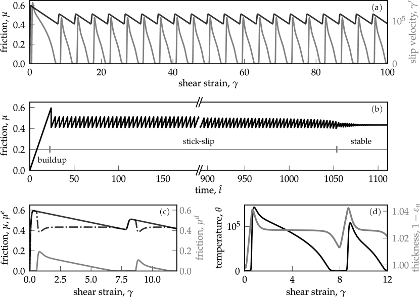
Figure 7: Response of the Terracotta-spring model: (a) friction coefficient $\mu$ and non-dimensional slip velocity (or non-dimensional strain rate) $\gamma^{\prime}$ as functions of the shear strain $\gamma$; (b) friction coefficient $\mu$ during the non-dimensional time $\hat{t}$ (b); (c) a focus view on the evolution of various components of the friction coefficient; and (d) a focus view highlighting the synchronicity of the meso-temperature $\theta$ and the non-dimensional thickness, $1+\varepsilon_{n}$. Results refer to $v_{\infty}=1$ cm/year, and initial conditions: $h^{0}=0.1$ mm, $\phi^{0}=0.71$, and $\sigma_{n}=40$ MPa.

In summary, the proposed Terracotta-spring model enables to study the nucleation of earthquakes, with the development of well-defined and persistent stick-slip sliding, which is synchronised with the evolution of the meso-temperature and the evolution of the shear zone thickness, with an intermittent pattern. To investigate the transition from stick-slip cycle to smooth sliding, cf. Figure 7(b), we considered a critically-damped scenario ($\zeta=1$). In this case, the model yields the exact same dynamic behaviour, where persistent stick-slip cycles develop, with only a time-increasing lag in the recurrence of the periodic seismic events of the order of $0.03$ at $\hat{t}=100$. Therefore, in the following we shall consider the model without the dashpot using $\zeta=0$, for simplicity.

5.2 Influence of physical parameters

Here, we investigate the influence of physical parameters and namely the slip zone thickness, the solid fraction, the normal stress, and the far-field velocity. While the influence of some of these parameters has been extensively studied using previous rate-and-state and micromechanically-inspired friction laws, as well as using high-fidelity simulations including finite element and discrete element methods, the effects of other physical parameters remain challenging to capture with simplified one-dimensional models. The objective here is twofold: (1) to examine the impact of key physical quantities which were not well studied in the past, such as slip zone thickness, and (2) to assess whether the newly proposed friction law exhibits trends consistent with those observed in experiments but also in conventional rate-and-state friction laws, thereby validating its relevance in capturing known frictional mechanisms.

5.2.1 Slip zone thickness, $h$

In contrast with conventional state-of-the-art friction models that treat friction as a surface phenomenon, a key feature of the Terracotta friction law is the incorporation of a finite slip zone thickness. In the Terracotta-spring model, the thickness evolves during both the earthquake nucleation and slip, and its initial value appears to significantly influence the frictional instabilities, limit cycles, and stress drops associated with each seismic event. It is also worth noticing that the current model does not account for phenomena such as particle breakage, thermal pressurization, flash heating, or frictional melting, each of which is thought to influence the shear zone’s thickness and fault surface roughness evolution <for an extensive review, see¿faulkner2010review,collins2020cosserat,stathas2023fault. Nonetheless, the results shed light on additional important phenomena that complement those listed above.

Following the experimental evidence collected and presented by rice2006, we select initial thicknesses between $10\text{ \textmu m}\geq h^{0}\geq 10$ mm. The parametric study is conducted per metre unit length of the fault gouge segment, leading to a non-dimensional thickness parameter $10^{-5}\geq\epsilon\geq 10^{-2}$. Figure 8 shows the phase portraits (left and centre) of the friction coefficient with respect to the slip velocity, $\gamma^{\prime}$, and the ratio of normal-to-slip velocity, $\varepsilon_{n}^{\prime}/\gamma^{\prime}$, as well as the friction coefficient as a function of the accumulated slip (right) for decreasing thicknesses (from top to bottom). For the relatively largest thickness, i.e., $\epsilon=10^{-2}$ ($h^{0}=10$ mm), the model predicts an isolated seismic event followed by a smooth, stable sliding. When the initial thickness decreases to $\epsilon=10^{-3}$ ($h^{0}=1$ mm), the model exhibits stick-slip behaviour with rapidly decreasing amplitudes, which ultimately converge to the same fixed-point attractor as in the $\epsilon=10^{-2}$ case. The attractor is equal to $\mu\sim M/\sqrt{3}$ and stems from the critical state limits that are embodied in the Terracotta friction law. For even smaller initial thicknesses, i.e., $\epsilon\leq 10^{-4}$ ($h^{0}\leq 100$ µm), the model predicts sustained stick-slip limit cycles with amplitudes inversely related to the thickness. In this latter scenario, the limit cycles also appear in the normal-to-slip velocity, demonstrating that the coupling between frictional slip and the underlying compaction/dilation of the fault gouge actively participates in the dynamics of earthquakes.

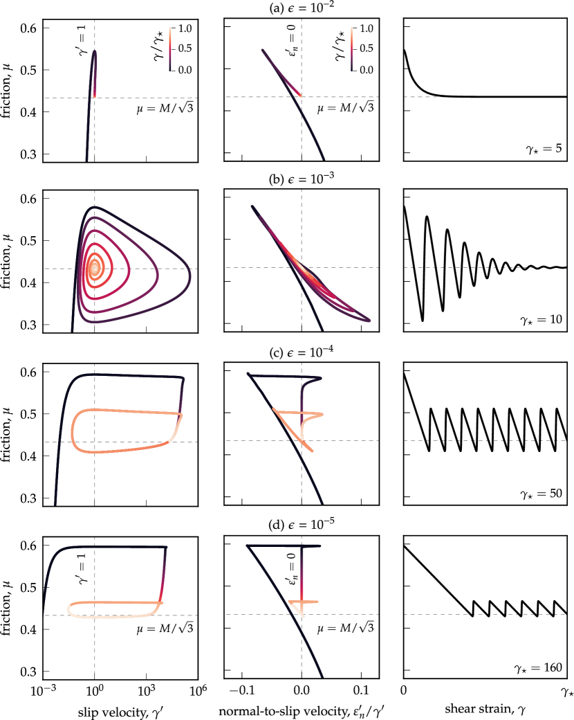
Figure 8: Influence of the non-dimensional gouged shear zone thickness, $\epsilon$, on earthquake dynamics. Evolution of the friction coefficient with respect to the non-dimensional slip velocity (left), the normal-to-slip velocity (centre), and shear strain (right) under decreasing shear zone thickness (from top to bottom): (a) $\epsilon=10^{-2}$, (b) $\epsilon=10^{-3}$, (c) $\epsilon=10^{-4}$, and (d) $\epsilon=10^{-5}$. Results refer to slip velocity of $v_{\infty}=1$ cm/year and initial conditions of $\phi^{0}=0.71$ and $\sigma_{n}=40$ MPa.

The results are further analysed and summarised in Figure 9 which shows the evolution of the friction drops and their recurrence intervals as function of the gouged shear zone thickness. As this thickness decreases, the non-dimensional recurrence period of the seismic events $\hat{t}_{r}$ increases. However the physical (dimensional) recurrence interval, $t_{r}$, decreases at the decreasing of the thickness within the stick-slip region. The friction drops are separated into two categories: the primary, typically larger drop, $\Delta\mu_{p}$, and subsequent drops, $\Delta\mu$ that, in the case of stick-slip behaviour, correspond to the limit cycle amplitude (also refer to Figure 7). The results suggest that there is a critical shear zone thickness that produces the largest stress drop. For larger $\epsilon$, the friction drops decrease rapidly as stick-slip transitions to stable, aseismic sliding. Similarly, as $\epsilon$ decreases, the friction drops for subsequent limit cycles approach zero, reflecting the decreasing amplitude of stick-slip events, while the primary drop reaches an asymptote, $\Delta\mu_{p}\sim 0.16$, independently of $\epsilon$.

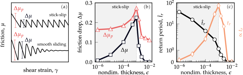
Figure 9: Influence of the non-dimensional gouged shear zone thickness, $\epsilon$, on earthquake characteristics. From left to right: (a) identification of the friction drops, $\Delta\mu_{p}$ and $\Delta\mu$, for stick-slip and smooth sliding, (b) evolution of the friction drops, and (c) return period, $\hat{t}_{r}$ ($t_{r}$), as s function of $\epsilon$. Results refer to slip velocity of $v_{\infty}=1$ cm/year and initial conditions of $\phi^{0}=0.71$ and $\sigma_{n}=40$ MPa.

The above results gather new insights on how stick-slip behaviour and nucleation of earthquakes are strongly related to the shear zone thickness. Note that the negative proportionality in the friction drops and return intervals at increasing initial thicknesses is in agreement with laboratory test of synthetic granular fault gouges Lyu . (2019).

5.2.2 Solid fraction, $\phi$

Next, we examine the impact of the initial solid fraction on the seismic response. Figure 10 presents these results in terms of the $\mu-\gamma^{\prime}$ limit cycles, the magnitude of friction drops, and the return interval. Figure 10(a) shows that the limit cycle attractor remains independent of $\phi^{0}$, leading to a constant $\Delta\mu$ and return interval $\hat{t}_{r}$, respectively in Figures 10(b,c). However, the initial solid fraction influences the primary friction drop, with two different trends emerging. For $\phi^{0}$ higher than the threshold for a normally consolidated gouge, $\phi_{c}$, the initial friction drop $\Delta\mu_{p}$ increases with increasing $\phi^{0}$, where $\phi_{c}\sim 0.65$ is obtained by requiring $p_{c}(\phi)/p=1$. This aligns with the concept of critical state in soil mechanics, where denser materials display a more pronounced stress peak followed by strain softening before reaching critical state. In contrast, for looser states ($\phi^{0}\leq\phi_{c}$), the friction drop increases as $\phi^{0}$ decreases, due to stress adjustments during the elastic buildup that precedes the primary drop and enabling the compaction of the gouge.

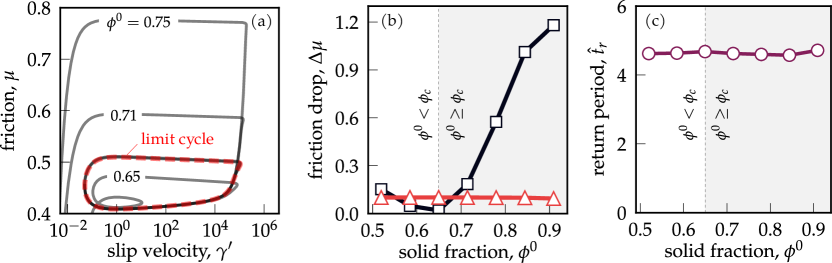
Figure 10: Influence of the solid fraction, $\phi^{0}$, on earthquake dynamics and characteristics under constant normal stress $\sigma_{n}=40$ MPa: (a) phase portrait of the friction versus the non-dimensional slip velocity and limit cycle, (b) friction drops, and (c) return period in terms of $\phi^{0}$. Results refer to $v_{\infty}=1$ cm/year and initial conditions of $h^{0}=0.1$ mm shear band thickness. The value of the solid fraction corresponding to the normally consolidated scenario is $\phi_{c}=0.65$.

5.2.3 Normal stress, $\sigma_{n}$

The results in Figure 11 shows responses for various constant normal stress, $\sigma_{n}$ from 5 to 640 MPa. As $\sigma_{n}$ decreases, both the primary and cyclic friction drops increase, in agreement with experimental evidence Saffer  Marone (2003); Numelin . (2007). In particular, Figure 11(a) shows that the limit cycles tend to expand toward higher cyclic friction values and contract at lower slip velocities as $\sigma_{n}$ decreases. The return period instead increases exponentially with increasing normal stress.

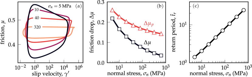
Figure 11: Influence of the normal stress, $\sigma_{n}$, on earthquake dynamics and characteristics under a constant overconsolidation ratio $p/p_{c}\sim 4$: (a) stick-slip limit cycles, (b) friction drops, and (c) return period in terms of $\sigma_{n}$. Results refer to $v_{\infty}=1$ cm/year, and initial conditions of $h^{0}=0.1$ mm.

To further assess the predictive capabilities of the Terracotta-spring model relative to other models, simulations, and data from natural and induced seismicity, we temporarily move from the non-dimensional analysis to consider physical variations of dimensional parameters. Figure 12(a) shows an example of a slip-weakening curve obtained from the new model and definition of energetic parts of the budget per unit area during a seismic event, for $\sigma_{n}=40$ MPa. As conventionally referred to in geophysics, the energy budget comprises the three contributions explained in Figure 12(a) and identified as: (1) released elastic energy, $E_{R}$, (2) fracture energy, $E_{G}$, and (3) frictional energy, $E_{F}$ Kanamori  Brodsky (2004); Kanamori  Rivera (2006). For $\sigma_{n}=40$ MPa, we find $E_{G}=0.21$ J/m², $E_{F}=170$ J/m², and $E_{R}=0.04$ J/m².

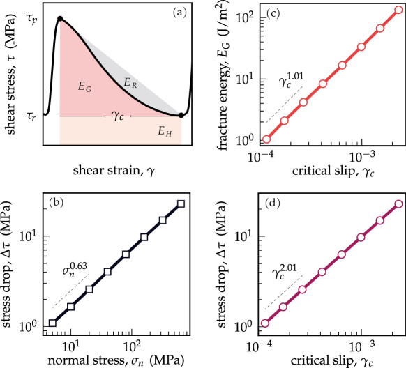
Figure 12: Influence of the normal stress on fault energetics and statistics: (a) schematic representation of the energy budget; (b) stress drop as a function of the normal stress; and (c,d) fracture energy and stress drop over $\gamma_{c}$ defined in (a).

Figure 12(b) shows a power law increase of the cyclic stress drops with normal stress, which well compares with previous discrete element method numerical simulations and experimental studies on gouges Passelègue . (2016); Bedford  Faulkner (2021); Bai  Konietzky (2022). Here, we get $\Delta\tau\propto\sigma_{n}^{0.63}$. Furthermore, the model predictions for the relationships between the stress drops, $\Delta\tau$, and fracture energy, $E_{G}$, with respect to the critical slip, $\gamma_{c}$, align well with prior experimental studies conducted on smooth and gouge faults Aubry . (2018); Passelègue . (2016); Ohnaka (2003); Passelègue . (2017); Sellers . (2003), rock fracturing Yoshimitsu . (2014), acoustic emission data Goodfellow  Young (2014), and discrete element method numerical simulations Kato (2012); Bai  Konietzky (2022); Casas . (2023). Both $\Delta\tau$ and $E_{G}$ well match a power law with slip: $\Delta\tau\propto\gamma_{c}^{1.016}$ and $E_{G}\propto\gamma_{c}^{2.008}$. A first-order approximation of the fracture energy, given by the triangular area $(\tau_{p}-\tau_{r})/\gamma_{c}$, suggests $E_{G}\propto\Delta\tau\gamma_{c}=\gamma_{c}^{2.016}$, which indicates minimal released energy, $E_{R}$.

5.2.4 Far-field velocity, $v_{\infty}$

Finally, we study the influence of the tectonic far-field velocity, $v_{\infty}$, by testing over six order of magnitude variations, i.e., $10^{-5}\leq v_{\infty}\leq 50$ µm/s. Figure 13 summarises the results which are in agreement with the well-known dependence of fault gouges on $v_{\infty}$ Scholz (2019); Kanamori  Brodsky (2004); Y. Gu  Wong (1991, 1994).

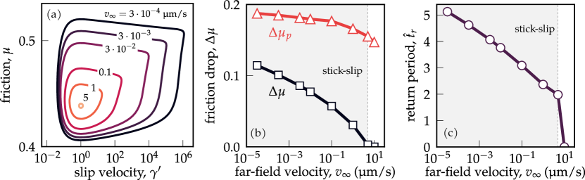
Figure 13: Influence of the far-field velocity, $v_{\infty}$ on fault energetics and statistics: (a) stick-slip limit cycles, (b) friction drops, and (c) return period versus $v_{\infty}$. Results refer to initial conditions of $h^{0}=0.1$ mm, $\phi^{0}=0.71$, and $\sigma_{n}=40$ MPa.

The far-field velocity determines the loading rate of the fault, and is found to directly influence the return period and indirectly affect the stress drops and stick-slip limit cycles. Higher velocities lead to faster stress accumulation, producing more frequent seismic events of lower magnitude. On the contrary, lower velocities yield slower loading rates, which in turns produce larger return periods, with seismic events characterised by larger stress drops. This is true both for the primary stress drop, $\Delta\mu_{p}$, and the persistent periodic drops, $\Delta\mu$. It is worth noticing that at vary large velocities, the stick-slip limit cycles tend to converge to a fixed-point attractor at $\mu\sim M\sqrt{3}$.

The return interval and the far-field velocity are found to follow a power law, i.e., $v_{\infty}\propto t_{r}^{-1.08}$, as shown in Figure 14 and in agreement with existing natural seismicity data and laboratory tests Beeler . (2001).

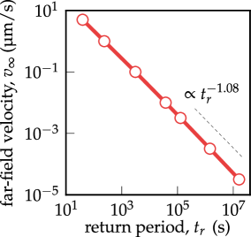
Figure 14: Influence of the far-field velocity, $v_{\infty}$: relationships between $v_{\infty}$ and return period, $t_{r}$.

6   Conclusions

This study develops a new pathway to study the frictional behaviour of fault gouges that is grounded on hydrodynamic principles from theoretical physics Landau  Lifshitz (2013) that considers the way energy flows in heterogeneous media through the use of thermal and meso-related temperatures Jiang  Liu (2009); Einav  Liu (2023). In particular, we built upon the hydrodynamic Terracotta model of clay Wiebicke  Einav (2024). Initially formulated for triaxial loading, this paper established its tensorially generalised form, in order to solve the particular loading conditions of directly sheared fault gouges. Unlike previous models, this pathway ensures an objective evaluation that does not engineer the friction law against observational trends. As a result, the new friction law accounts for the volumetric response of the materials, and directly captures the dependence of fault gouge dynamics on thickness, normal stress and solid fraction, as well as explains for the first time analytically the buildups of an elastic stress towards first rupture.

The performance of the Terracotta friction law was validated against laboratory experiments of clay-rich fault gouges across various scenarios, including velocity stepping, varying normal stress, and gouge compaction Saffer  Marone (2003); Ashman  Faulkner (2023); Bedford . (2022). By integrating this friction law with a conventional spring-dashpot representation of the host rock, the full seismic cycle was simulated, showcasing both shear stress accumulation and earthquake nucleation. The numerical results of this Terracotta-spring model successfully captured several well-established trends observed in laboratory experiments, advanced simulations, as well as natural and induced seismicity. Key result includes the model predictions of the finding by lyu2019mechanics of the dependence of friction drops and return intervals on the initial gouge thickness. Furthermore, the same Terracotta-spring model offers insights into behaviours that await experimental studies, including: (1) the existence of a critical shear zone thickness that maximises stress drops; and (2) the independence of the return periods on the initial solid fraction of the gouge.

The newly developed friction law represents a significant step beyond phenomenological rate-and-state laws, in that it enriches understanding of the physics of friction of fault gouges. Thanks to the physical generality of the hydrodynamic procedure Landau  Lifshitz (2013); Jiang  Liu (2009) and the simplicity of Terracotta Wiebicke  Einav (2024), the use of the new friction law should be applicable to model general heterogeneous geomaterials, beyond just clay-rich gouges as done in this paper. As show in einav2023hydrodynamics,chen2023hydrodynamic, the hydrodynamic procedure can accurately describe multi-physics coupled phenomena, which have important implications on fault dynamics <see¿[among others]rice2006,veveakis2012modeling,rattez2018importanceI,stathas2023fault.

While in this paper the initial thickness of the fault gouge was taken as a parameter, the evolution equation of the meso-temperature in the complete Terracotta model showcases dependence on its second gradient that naturally introduces an evolving length scale to continuum mechanics. With that, it is anticipated that the Terracotta constitutive model could help addressing both the genesis of faults – through the localisation of strain, kinetic fluctuations (meso-temperature), and thermal pressurisation <among others, see¿stathas2023fault – and the subsequent evolution of rate- and state-dependent earthquake cycles.

Appendix A: Numerical implementation

The numerical implementation of Terracotta friction law, Equations (22-24), is developed in Python, by solving the initial value problem specified by the evolution equations for the state variables and the time derivative of the shear stress, Equation (22), given the initial conditions in Equation (21), using the solve_ivp package from SciPy library Virtanen . (2020). The time derivative of the shear stress is obtained by time differentiation of Equation (22):

$$\dot{\tau}=\frac{\partial\tau}{\partial\varepsilon_{v}^{e}}\dot{\varepsilon}_{v}^{e}+\frac{\partial\tau}{\partial\gamma^{e}}\dot{\gamma}^{e}+\frac{\partial\tau}{\partial T_{m}}\dot{T}_{m}+\frac{\partial\tau}{\partial h}v_{n}+\frac{\partial\tau}{\partial v}\dot{v},$$ (30)

where $\dot{\varepsilon}_{v}^{e}$, $\dot{\gamma}^{e}$, $\dot{T}_{m}$, and $v_{n}$ (or $\dot{h}$) are prescribed by Equations (23) and (24). The slip acceleration, $\dot{v}$, is approximated with a backward finite-difference scheme.

The solution of the initial value problem is driven by the prescribed time evolution of the shear strain rate, $\dot{\gamma}$ (or equivalently, the slip velocity, $v$) and the imposed value of the normal stress, $\sigma_{n}$. To guarantee a constant value of the normal stress, a root-finding algorithm is used to identify the normal-strain rate, $\dot{\varepsilon}_{n}$ (or, $v_{n}$), to yield

$$\dot{\sigma}_{n}=\frac{\partial{\sigma}_{n}}{\partial\varepsilon_{v}^{e}}\dot{\varepsilon}_{v}^{e}+\frac{\partial{\sigma}_{n}}{\partial\varepsilon_{s}^{e}}\dot{\varepsilon}_{s}^{e}+\frac{\partial{\sigma}_{n}}{\partial\varepsilon_{n}^{e}}\dot{\varepsilon}_{n}^{e}+\frac{\partial{\sigma}_{n}}{\partial T_{m}}\dot{T}_{m}+\frac{\partial{\sigma}_{n}}{\partial h}v_{n}+\frac{\partial{\sigma}_{n}}{\partial v_{n}}\dot{v}_{n}=0,$$ (31)

where the rates of the state variables are functions of the state, as well as the shear and normal strain rates. Equation (31) is numerically solved using the SciPy’s minimize package.

Further notice that in all simulations, the numerical implementation of Equation (24b) uses the initial thickness, $h^{0}$, rather than the current thickness, $h$, for the sake of simplicity. This assumption is confirmed by the results where the normal strain is found to be infinitesimal small, i.e., $\lesssim 5\%$.

The system of ordinary differential equations defining the initial value problem is numerically integrated using a fifth-order implicit Runge-Kutta method from the Radau IIA family Virtanen . (2020). Adaptive time stepping is employed, with absolute error tolerances varying between 10^-8 and 10^-12, to ensure that no significant differences are observed in the computed solutions.

The numerical implementation of the Terracotta-spring model, Equations (28), is analogous to that of the Terracotta friction law, with the only difference that the slip velocity, $\dot{\gamma}$, and acceleration $\ddot{\gamma}$, are defined by the solution of the balance equation of the Terracotta-spring-dashpot system, cf. Equation (28a). For more details, we refer to the code Masi  Einav (2024).

Data Availability Statement

The experimental data sets used for the validation of the model were obtained directly from the corresponding works. The software for reproducing the results presented in this work will be made publicly available at github.

Notation

Einstein’s summation is implied for repeated indices $i,j=1,2,3$

$a,b,c$

Volumetric, off-diagonal, and deviatoric plastic transport coefficients

$d_{\infty},d$

Far-field and gouge’s slip displacements

$D$

Characteristic length

$e^{e}_{ij}=\varepsilon^{e}_{ij}-\smash{\frac{\varepsilon^{e}_{v}}{3}}\delta_{ij}$

Deviatoric elastic strain tensor

$f_{i},f^{m}_{i}$

Thermal and meso-related entropy currents

$\tilde{G},\tilde{K}$

Intrinsic shear and bulk moduli

$G_{*}$

Host rock shear modulus

$h$

Gouged shear zone thickness

$m$

Mobilised mass

$M$

Critical stress ratio

$L$

Gouge’s length

$p=\smash{\frac{\sigma_{ii}}{3}}$

Total pressure

$p_{c}(\phi)$

Isotropic compression line

$p_{I}$

Constant defining the isotropic compression line

$p^{d}$

Viscous pressure

$p^{e}$

Elastic pressure

$p^{T}$

Thermodynamic pressure

$q=\smash{\sqrt{\nicefrac{{3}}{{2}}\;s_{ij}s_{ij}}}$

Deviatoric total stress (invariant)

$q^{d}$

Viscous deviatoric stress

$q^{e}$

Elastic deviatoric stress

$R,R_{m}$

Thermal and meso-related entropy productions

$s,s_{m}$

Thermal and meso-related entropies

$s_{ij}=\sigma_{ij}-p\delta_{ij}$

Deviatoric stress tensor

$t$

Time

$\mathscr{T}$

Characteristic time

$\hat{t}$

Non-dimensional time

$T,T_{m}$

Thermal temperature and meso-temperature

$u,u^{e},u^{m}$

Total, elastic, and meso-related internal energy densities

$v_{i}$

Velocity vector

$v,v_{n},v_{\infty}$

Slip, normal, and far-field velocities

$\mathbb{X}^{d}_{ijkl},\mathbb{X}^{p}_{ijkl}$

Viscous and plastic transport coefficients

$\Box^{0}$

Initial value of variable $\Box$

$\dot{\Box}=\frac{\partial x}{\partial t}$

Derivative of variable $\Box$ with respect to time $t$

$\Box^{\prime}=\frac{\partial\Box}{\partial\hat{t}}$

Derivative of the variable $\Box$ with respect to the non-dimensional time $\hat{t}$

$\nabla_{i}\square=\frac{\partial\Box}{\partial x_{i}}$

Gradient of the scalar variable $\Box$

$\nabla_{i}\square_{i}=\frac{\partial\square_{i}}{\partial x_{i}}$

Divergence of the vectorial variable $\square_{i}$

$\nabla^{2}_{i}\Box=\frac{\partial^{2}\Box}{\partial x_{i}^{2}}$

Laplacian of the scalar variable $\Box$

$\gamma^{e}$

Elastic shear strain

$\dot{\gamma},\dot{\gamma}^{e}$

Total and elastic shear strain rates

$\Gamma$

Fixed coefficient that sets the unit of the meso-temperature

$\bar{\eta}$

Energy sink coefficient

$\eta$

Constant parameter specifying the energy sink

$\delta_{ij}$

Kronecker delta

$\varepsilon^{e}_{ij}$

Elastic strain tensor

$\varepsilon^{e}_{v}=\varepsilon^{e}_{ii}$

Volumetric stress invariant

$\varepsilon_{s}^{e}=\sqrt{\nicefrac{{2}}{{3}}\;\smash{e^{e}_{ij}e^{e}_{ij}}}$

Deviatoric elastic strain invariant

$\dot{\varepsilon}^{e}_{ij},\dot{\varepsilon}_{ij},\dot{\varepsilon}_{ij}^{p}$

Elastic, total, and plastic strain-rate tensors

${\varepsilon}^{e}_{n},{\varepsilon}^{e}_{\ell}$

Normal and longitudinal elastic strains

$\varepsilon_{n}$

Normal strain

$\dot{\varepsilon}_{n},\dot{\varepsilon}_{\ell}$

Normal and longitudinal strain rates

$\mu$

Friction coefficient

$\phi$

Solid fraction

$\phi_{I}$

Solid fraction of the isotropic compression line, at $p=1$ kPa

$\lambda$

Slope of the isotropic compression line

$\rho$

Bulk density

$\rho_{s}$

Solid density

$\rho_{*}$

Host rock’s bulk density

$\sigma_{ij}$

Total stress tensor

$\sigma^{d}_{ij}$

Viscous stress tensor

$\sigma^{e}_{ij}$

Elastic stress tensor

$\sigma_{n},\sigma_{\ell},\tau$

Normal, longitudinal, and shear stresses

$\Theta$

Characteristic meso-temperature

$\omega$

Position of the critical state line

$\zeta$

Damping ratio

References

- Alaei \BOthers. (\APACyear2021) \APACinsertmetastaralaei2021hydrodynamic{APACrefauthors}Alaei, E., Marks, B.\BCBL \BBA Einav, I. \APACrefYearMonthDay2021. \BBOQ\APACrefatitleA hydrodynamic-plastic formulation for modelling sand using a minimal set of parameters A hydrodynamic-plastic formulation for modelling sand using a minimal set of parameters.\BBCQ \APACjournalVolNumPagesJournal of the Mechanics and Physics of Solids151104388. {APACrefDOI} \doihttps://doi.org/10.1016/j.jmps.2021.104388 \PrintBackRefs\CurrentBib
- Ashman \BBA Faulkner (\APACyear2023) \APACinsertmetastarashman2023effect{APACrefauthors}Ashman, I.\BCBT \BBA Faulkner, D. \APACrefYearMonthDay2023. \BBOQ\APACrefatitleThe effect of clay content on the dilatancy and frictional properties of fault gouge The effect of clay content on the dilatancy and frictional properties of fault gouge.\BBCQ \APACjournalVolNumPagesJournal of Geophysical Research: Solid Earth1284e2022JB025878. {APACrefDOI} \doihttps://doi.org/10.1029/2022JB025878 \PrintBackRefs\CurrentBib
- Aubry \BOthers. (\APACyear2018) \APACinsertmetastaraubry2018frictional{APACrefauthors}Aubry, J., Passelègue, F\BPBIX., Deldicque, D., Girault, F., Marty, S., Lahfid, A.\BDBLSchubnel, A. \APACrefYearMonthDay2018. \BBOQ\APACrefatitleFrictional heating processes and energy budget during laboratory earthquakes Frictional heating processes and energy budget during laboratory earthquakes.\BBCQ \APACjournalVolNumPagesGeophysical Research Letters452212–274. {APACrefDOI} \doihttps://doi.org/10.1029/2018GL079263 \PrintBackRefs\CurrentBib
- Bai \BBA Konietzky (\APACyear2022) \APACinsertmetastarbai2022numerical{APACrefauthors}Bai, Q.\BCBT \BBA Konietzky, H. \APACrefYearMonthDay2022. \BBOQ\APACrefatitleNumerical Insight Into Energy Partitioning During Stick-Slip Events Based on the Framework of Rate-and-State Friction Law Numerical insight into energy partitioning during stick-slip events based on the framework of rate-and-state friction law.\BBCQ \APACjournalVolNumPagesGeophysical Research Letters499e2021GL096677. {APACrefDOI} \doihttps://doi.org/10.1029/2021GL096677 \PrintBackRefs\CurrentBib
- Bedford \BBA Faulkner (\APACyear2021) \APACinsertmetastarbedford2021role{APACrefauthors}Bedford, J\BPBID.\BCBT \BBA Faulkner, D\BPBIR. \APACrefYearMonthDay2021. \BBOQ\APACrefatitleThe role of grain size and effective normal stress on localization and the frictional stability of simulated quartz gouge The role of grain size and effective normal stress on localization and the frictional stability of simulated quartz gouge.\BBCQ \APACjournalVolNumPagesGeophysical Research Letters487e2020GL092023. {APACrefDOI} \doihttps://doi.org/10.1029/2020GL092023 \PrintBackRefs\CurrentBib
- Bedford \BOthers. (\APACyear2022) \APACinsertmetastarbedford2022fault{APACrefauthors}Bedford, J\BPBID., Faulkner, D\BPBIR.\BCBL \BBA Lapusta, N. \APACrefYearMonthDay2022. \BBOQ\APACrefatitleFault rock heterogeneity can produce fault weakness and reduce fault stability Fault rock heterogeneity can produce fault weakness and reduce fault stability.\BBCQ \APACjournalVolNumPagesNature Communications131326. {APACrefDOI} \doihttps://doi.org/10.1038/s41467-022-27998-2 \PrintBackRefs\CurrentBib
- Beeler \BOthers. (\APACyear2001) \APACinsertmetastarbeeler2001earthquake{APACrefauthors}Beeler, N., Hickman, S.\BCBL \BBA Wong, T\BHBIF. \APACrefYearMonthDay2001. \BBOQ\APACrefatitleEarthquake stress drop and laboratory-inferred interseismic strength recovery Earthquake stress drop and laboratory-inferred interseismic strength recovery.\BBCQ \APACjournalVolNumPagesJournal of Geophysical Research: Solid Earth106B1230701–30713. {APACrefDOI} \doihttps://doi.org/10.1029/2000JB900242 \PrintBackRefs\CurrentBib
- Bigaroni \BOthers. (\APACyear2023) \APACinsertmetastarbigaroni2023frictional{APACrefauthors}Bigaroni, N., Scuderi, M\BPBIM., Cappa, F., Guglielmi, Y., Nussbaum, C., Aldega, L.\BDBLCollettini, C. \APACrefYearMonthDay2023. \BBOQ\APACrefatitleFrictional properties of Opalinus Clay: influence of humidity, normal stress and grain size on frictional stability Frictional properties of Opalinus Clay: influence of humidity, normal stress and grain size on frictional stability.\BBCQ \APACjournalVolNumPagesGeophysical Journal International2331211–228. {APACrefDOI} \doihttps://doi.org/10.1093/gji/ggac457 \PrintBackRefs\CurrentBib
- Byerlee \BBA Summers (\APACyear1976) \APACinsertmetastarbyerlee1976note{APACrefauthors}Byerlee, J.\BCBT \BBA Summers, R. \APACrefYearMonthDay1976. \BBOQ\APACrefatitleA note on the effect of fault gouge thickness on fault stability A note on the effect of fault gouge thickness on fault stability.\BBCQ \BIn \APACrefbtitleInternational Journal of Rock Mechanics and Mining Sciences & Geomechanics Abstracts International journal of rock mechanics and mining sciences & geomechanics abstracts (\BVOL 13, \BPGS 35–36). {APACrefDOI} \doihttps://doi.org/10.1016/0148-9062(76)90226-6 \PrintBackRefs\CurrentBib
- Carpenter \BOthers. (\APACyear2014) \APACinsertmetastarcarpenter2014{APACrefauthors}Carpenter, B\BPBIM., Scuderi, M\BPBIM., Collettini, C.\BCBL \BBA Marone, C. \APACrefYearMonthDay2014. \BBOQ\APACrefatitleFrictional heterogeneities on carbonate-bearing normal faults: Insights from the Monte Maggio Fault, Italy Frictional heterogeneities on carbonate-bearing normal faults: Insights from the monte maggio fault, italy.\BBCQ \APACjournalVolNumPagesJournal of Geophysical Research: Solid Earth119129062-9076. {APACrefDOI} \doihttps://doi.org/10.1002/2014JB011337 \PrintBackRefs\CurrentBib
- Casas \BOthers. (\APACyear2023) \APACinsertmetastarhttps://doi.org/10.1029/2022JB025666{APACrefauthors}Casas, N., Mollon, G.\BCBL \BBA Daouadji, A. \APACrefYearMonthDay2023. \BBOQ\APACrefatitleInfluence of Grain-Scale Properties on Localization Patterns and Slip Weakening Within Dense Granular Fault Gouges Influence of grain-scale properties on localization patterns and slip weakening within dense granular fault gouges.\BBCQ \APACjournalVolNumPagesJournal of Geophysical Research: Solid Earth1283e2022JB025666. {APACrefDOI} \doihttps://doi.org/10.1029/2022JB025666 \PrintBackRefs\CurrentBib
- J. Chen \BBA Niemeijer (\APACyear2017) \APACinsertmetastarNiemeijer2017{APACrefauthors}Chen, J.\BCBT \BBA Niemeijer, A\BPBIR. \APACrefYearMonthDay2017. \BBOQ\APACrefatitleSeismogenic Potential of a Gouge-filled Fault and the Criterion for Its Slip Stability: Constraints From a Microphysical Model Seismogenic potential of a gouge-filled fault and the criterion for its slip stability: Constraints from a microphysical model.\BBCQ \APACjournalVolNumPagesJournal of Geophysical Research: Solid Earth122129658-9688. {APACrefDOI} \doihttps://doi.org/10.1002/2017JB014228 \PrintBackRefs\CurrentBib
- J. Chen \BBA Spiers (\APACyear2016) \APACinsertmetastarspiers2016{APACrefauthors}Chen, J.\BCBT \BBA Spiers, C\BPBIJ. \APACrefYearMonthDay2016. \BBOQ\APACrefatitleRate and state frictional and healing behavior of carbonate fault gouge explained using microphysical model Rate and state frictional and healing behavior of carbonate fault gouge explained using microphysical model.\BBCQ \APACjournalVolNumPagesJournal of Geophysical Research: Solid Earth121128642-8665. {APACrefDOI} \doihttps://doi.org/10.1002/2016JB013470 \PrintBackRefs\CurrentBib
- T. Chen \BBA Lapusta (\APACyear2009) \APACinsertmetastarchenlapusta2009{APACrefauthors}Chen, T.\BCBT \BBA Lapusta, N. \APACrefYearMonthDay2009. \BBOQ\APACrefatitleScaling of small repeating earthquakes explained by interaction of seismic and aseismic slip in a rate and state fault model Scaling of small repeating earthquakes explained by interaction of seismic and aseismic slip in a rate and state fault model.\BBCQ \APACjournalVolNumPagesJournal of Geophysical Research: Solid Earth114B1. {APACrefDOI} \doihttps://doi.org/10.1029/2008JB005749 \PrintBackRefs\CurrentBib
- Y. Chen \BOthers. (\APACyear2023) \APACinsertmetastarchen2023hydrodynamic{APACrefauthors}Chen, Y., Guillard, F.\BCBL \BBA Einav, I. \APACrefYearMonthDay2023. \BBOQ\APACrefatitleA hydrodynamic model for chemo-mechanics of poroelastic materials A hydrodynamic model for chemo-mechanics of poroelastic materials.\BBCQ \APACjournalVolNumPagesGéotechnique1–16. {APACrefDOI} \doihttps://doi.org/10.1680/jgeot.22.00260 \PrintBackRefs\CurrentBib
- Ciardo \BBA Viesca (\APACyear2024) \APACinsertmetastarciardo2024non{APACrefauthors}Ciardo, F.\BCBT \BBA Viesca, R\BPBIC. \APACrefYearMonthDay2024. \BBOQ\APACrefatitleNon-linear stability analysis of slip in a single-degree-of-freedom elastic system with frictional evolution laws spanning aging to slip Non-linear stability analysis of slip in a single-degree-of-freedom elastic system with frictional evolution laws spanning aging to slip.\BBCQ \APACjournalVolNumPagesarXiv preprint arXiv:2407.16846. {APACrefDOI} \doihttps://doi.org/10.48550/arXiv.2407.16846 \PrintBackRefs\CurrentBib
- Collins-Craft \BOthers. (\APACyear2020) \APACinsertmetastarcollins2020cosserat{APACrefauthors}Collins-Craft, N\BPBIA., Stefanou, I., Sulem, J.\BCBL \BBA Einav, I. \APACrefYearMonthDay2020. \BBOQ\APACrefatitleA Cosserat Breakage Mechanics model for brittle granular media A cosserat breakage mechanics model for brittle granular media.\BBCQ \APACjournalVolNumPagesJournal of the Mechanics and Physics of Solids141103975. {APACrefDOI} \doihttps://doi.org/10.1016/j.jmps.2020.103975 \PrintBackRefs\CurrentBib
- De Gennes \BBA Prost (\APACyear1993) \APACinsertmetastarde1993physics{APACrefauthors}De Gennes, P\BHBIG.\BCBT \BBA Prost, J. \APACrefYear1993. \APACrefbtitleThe physics of liquid crystals The physics of liquid crystals (\BNUM 83). \APACaddressPublisherOxford university press. {APACrefDOI} \doihttps://doi.org/10.1063/1.2808028 \PrintBackRefs\CurrentBib
- Dieterich (\APACyear1979) \APACinsertmetastardieterich1979modeling{APACrefauthors}Dieterich, J\BPBIH. \APACrefYearMonthDay1979. \BBOQ\APACrefatitleModeling of rock friction: 1. Experimental results and constitutive equations Modeling of rock friction: 1. experimental results and constitutive equations.\BBCQ \APACjournalVolNumPagesJournal of Geophysical Research: Solid Earth84B52161–2168. {APACrefDOI} \doihttps://doi.org/10.1029/JB084iB05p02161 \PrintBackRefs\CurrentBib
- Dieterich (\APACyear1981) \APACinsertmetastardieterich1981constitutive{APACrefauthors}Dieterich, J\BPBIH. \APACrefYearMonthDay1981. \BBOQ\APACrefatitleConstitutive properties of faults with simulated gouge Constitutive properties of faults with simulated gouge.\BBCQ \APACjournalVolNumPagesAmerican Geophysical Union24103–120. {APACrefDOI} \doihttps://doi.org/10.1029/GM024p0103 \PrintBackRefs\CurrentBib
- Einav \BBA Liu (\APACyear2018) \APACinsertmetastareinav2018hydrodynamic{APACrefauthors}Einav, I.\BCBT \BBA Liu, M. \APACrefYearMonthDay2018. \BBOQ\APACrefatitleHydrodynamic derivation of the work input to fully and partially saturated soils Hydrodynamic derivation of the work input to fully and partially saturated soils.\BBCQ \APACjournalVolNumPagesJournal of the Mechanics and Physics of Solids110205–217. {APACrefDOI} \doihttps://doi.org/10.1016/j.jmps.2017.10.004 \PrintBackRefs\CurrentBib
- Einav \BBA Liu (\APACyear2023) \APACinsertmetastareinav2023hydrodynamics{APACrefauthors}Einav, I.\BCBT \BBA Liu, M. \APACrefYearMonthDay2023. \BBOQ\APACrefatitleHydrodynamics of Non-Equilibrium Soil Water Retention Hydrodynamics of non-equilibrium soil water retention.\BBCQ \APACjournalVolNumPagesWater Resources Research591. {APACrefDOI} \doi10.1029/2022WR033409 \PrintBackRefs\CurrentBib
- Evans (\APACyear1990) \APACinsertmetastarevans1990thickness{APACrefauthors}Evans, J\BPBIP. \APACrefYearMonthDay1990. \BBOQ\APACrefatitleThickness-displacement relationships for fault zones Thickness-displacement relationships for fault zones.\BBCQ \APACjournalVolNumPagesJournal of structural geology1281061–1065. {APACrefDOI} \doihttps://doi.org/10.1016/0191-8141(90)90101-4 \PrintBackRefs\CurrentBib
- Faulkner \BOthers. (\APACyear2010) \APACinsertmetastarfaulkner2010review{APACrefauthors}Faulkner, D., Jackson, C., Lunn, R., Schlische, R., Shipton, Z., Wibberley, C.\BCBL \BBA Withjack, M. \APACrefYearMonthDay2010. \BBOQ\APACrefatitleA review of recent developments concerning the structure, mechanics and fluid flow properties of fault zones A review of recent developments concerning the structure, mechanics and fluid flow properties of fault zones.\BBCQ \APACjournalVolNumPagesJournal of Structural Geology32111557–1575. {APACrefDOI} \doihttp://doi.org/10.1016/j.jsg.2010.06.009 \PrintBackRefs\CurrentBib
- Goodfellow \BBA Young (\APACyear2014) \APACinsertmetastargoodfellow2014laboratory{APACrefauthors}Goodfellow, S.\BCBT \BBA Young, R. \APACrefYearMonthDay2014. \BBOQ\APACrefatitleA laboratory acoustic emission experiment under in situ conditions A laboratory acoustic emission experiment under in situ conditions.\BBCQ \APACjournalVolNumPagesGeophysical Research Letters41103422–3430. {APACrefDOI} \doihttps://doi.org/10.1002/2014GL059965 \PrintBackRefs\CurrentBib
- J\BHBIC. Gu \BOthers. (\APACyear1984) \APACinsertmetastargu1984slip{APACrefauthors}Gu, J\BHBIC., Rice, J\BPBIR., Ruina, A\BPBIL.\BCBL \BBA Simon, T\BPBIT. \APACrefYearMonthDay1984. \BBOQ\APACrefatitleSlip motion and stability of a single degree of freedom elastic system with rate and state dependent friction Slip motion and stability of a single degree of freedom elastic system with rate and state dependent friction.\BBCQ \APACjournalVolNumPagesJournal of the Mechanics and Physics of Solids323167–196. {APACrefDOI} \doihttps://doi.org/10.1016/0022-5096(84)90007-3 \PrintBackRefs\CurrentBib
- Y. Gu \BBA Wong (\APACyear1991) \APACinsertmetastargu1991{APACrefauthors}Gu, Y.\BCBT \BBA Wong, T\BHBIf. \APACrefYearMonthDay1991. \BBOQ\APACrefatitleEffects of loading velocity, stiffness, and inertia on the dynamics of a single degree of freedom Spring-Slider System Effects of loading velocity, stiffness, and inertia on the dynamics of a single degree of freedom spring-slider system.\BBCQ \APACjournalVolNumPagesJournal of Geophysical Research: Solid Earth96B1321677-21691. {APACrefDOI} \doihttps://doi.org/10.1029/91JB02271 \PrintBackRefs\CurrentBib
- Y. Gu \BBA Wong (\APACyear1994) \APACinsertmetastargu1994nonlinear{APACrefauthors}Gu, Y.\BCBT \BBA Wong, T\BHBIF. \APACrefYearMonthDay1994. \BBOQ\APACrefatitleNonlinear dynamics of the transition from stable sliding to cyclic stick-slip in rock Nonlinear dynamics of the transition from stable sliding to cyclic stick-slip in rock.\BBCQ \APACjournalVolNumPagesNonlinear dynamics and predictability of geophysical phenomena8315–35. {APACrefDOI} \doihttps://doi.org/10.1029/GM083p0015 \PrintBackRefs\CurrentBib
- Haines \BOthers. (\APACyear2013) \APACinsertmetastarhaines2013shear{APACrefauthors}Haines, S\BPBIH., Kaproth, B., Marone, C., Saffer, D.\BCBL \BBA Van der Pluijm, B. \APACrefYearMonthDay2013. \BBOQ\APACrefatitleShear zones in clay-rich fault gouge: A laboratory study of fabric development and evolution Shear zones in clay-rich fault gouge: A laboratory study of fabric development and evolution.\BBCQ \APACjournalVolNumPagesJournal of Structural Geology51206–225. {APACrefDOI} \doihttps://doi.org/10.1016/j.jsg.2013.01.002 \PrintBackRefs\CurrentBib
- Henann \BBA Kamrin (\APACyear2013) \APACinsertmetastarhenann2013predictive{APACrefauthors}Henann, D\BPBIL.\BCBT \BBA Kamrin, K. \APACrefYearMonthDay2013. \BBOQ\APACrefatitleA predictive, size-dependent continuum model for dense granular flows A predictive, size-dependent continuum model for dense granular flows.\BBCQ \APACjournalVolNumPagesProceedings of the National Academy of Sciences110176730–6735. {APACrefDOI} \doihttps://doi.org/10.1073/pnas.1219153110 \PrintBackRefs\CurrentBib
- Hetland \BOthers. (\APACyear2010) \APACinsertmetastarhetland2010{APACrefauthors}Hetland, E\BPBIA., Simons, M.\BCBL \BBA Dunham, E\BPBIM. \APACrefYearMonthDay2010. \BBOQ\APACrefatitlePost-seismic and interseismic fault creep I: model description Post-seismic and interseismic fault creep i: model description.\BBCQ \APACjournalVolNumPagesGeophysical Journal International181181-98. {APACrefDOI} \doihttps://doi.org/10.1111/j.1365-246X.2010.04522.x \PrintBackRefs\CurrentBib
- Ikari \BOthers. (\APACyear2016) \APACinsertmetastarikarietal2016{APACrefauthors}Ikari, M\BPBIJ., Carpenter, B\BPBIM.\BCBL \BBA Marone, C. \APACrefYearMonthDay2016. \BBOQ\APACrefatitleA microphysical interpretation of rate- and state-dependent friction for fault gouge A microphysical interpretation of rate- and state-dependent friction for fault gouge.\BBCQ \APACjournalVolNumPagesGeochemistry, Geophysics, Geosystems1751660-1677. {APACrefDOI} \doihttps://doi.org/10.1002/2016GC006286 \PrintBackRefs\CurrentBib
- Ikari \BOthers. (\APACyear2011) \APACinsertmetastar2011JB008264{APACrefauthors}Ikari, M\BPBIJ., Niemeijer, A\BPBIR.\BCBL \BBA Marone, C. \APACrefYearMonthDay2011. \BBOQ\APACrefatitleThe role of fault zone fabric and lithification state on frictional strength, constitutive behavior, and deformation microstructure The role of fault zone fabric and lithification state on frictional strength, constitutive behavior, and deformation microstructure.\BBCQ \APACjournalVolNumPagesJournal of Geophysical Research: Solid Earth116B8. {APACrefDOI} \doihttps://doi.org/10.1029/2011JB008264 \PrintBackRefs\CurrentBib
- Jiang \BBA Liu (\APACyear2009) \APACinsertmetastarjiang2009granular{APACrefauthors}Jiang, Y.\BCBT \BBA Liu, M. \APACrefYearMonthDay2009. \BBOQ\APACrefatitleGranular solid hydrodynamics Granular solid hydrodynamics.\BBCQ \APACjournalVolNumPagesGranular Matter11139–156. {APACrefDOI} \doihttps://doi.org/10.1007/s10035-009-0137-3 \PrintBackRefs\CurrentBib
- Kamrin \BBA Koval (\APACyear2012) \APACinsertmetastarkamrin2012nonlocal{APACrefauthors}Kamrin, K.\BCBT \BBA Koval, G. \APACrefYearMonthDay2012. \BBOQ\APACrefatitleNonlocal constitutive relation for steady granular flow Nonlocal constitutive relation for steady granular flow.\BBCQ \APACjournalVolNumPagesPhysical review letters10817178301. {APACrefDOI} \doihttps://doi.org/10.1103/PhysRevLett.108.178301 \PrintBackRefs\CurrentBib
- Kanamori \BBA Brodsky (\APACyear2004) \APACinsertmetastarkanamori2004physics{APACrefauthors}Kanamori, H.\BCBT \BBA Brodsky, E\BPBIE. \APACrefYearMonthDay2004. \BBOQ\APACrefatitleThe physics of earthquakes The physics of earthquakes.\BBCQ \APACjournalVolNumPagesReports on progress in physics6781429. {APACrefDOI} \doihttps://doi.org/10.1088/0034-4885/67/8/R03 \PrintBackRefs\CurrentBib
- Kanamori \BBA Rivera (\APACyear2006) \APACinsertmetastarkanamori2006energy{APACrefauthors}Kanamori, H.\BCBT \BBA Rivera, L. \APACrefYearMonthDay2006. \BBOQ\APACrefatitleEnergy partitioning during an earthquake Energy partitioning during an earthquake.\BBCQ \APACjournalVolNumPagesGeophysical Monograph Series1703–13. {APACrefDOI} \doihttps://doi.org/10.1029/170GM03 \PrintBackRefs\CurrentBib
- Kato (\APACyear2012) \APACinsertmetastarkato2012dependence{APACrefauthors}Kato, N. \APACrefYearMonthDay2012. \BBOQ\APACrefatitleDependence of earthquake stress drop on critical slip-weakening distance Dependence of earthquake stress drop on critical slip-weakening distance.\BBCQ \APACjournalVolNumPagesJournal of Geophysical Research: Solid Earth117B1. {APACrefDOI} \doihttps://doi.org/10.1029/2011JB008359 \PrintBackRefs\CurrentBib
- Landau \BBA Lifshitz (\APACyear2013) \APACinsertmetastarlandau2013statistical{APACrefauthors}Landau, L\BPBID.\BCBT \BBA Lifshitz, E\BPBIM. \APACrefYear2013. \APACrefbtitleStatistical Physics Statistical physics (\BVOL 5). \APACaddressPublisherElsevier. {APACrefDOI} \doihttps://doi.org/10.1016/C2009-0-24487-4 \PrintBackRefs\CurrentBib
- Lapusta \BOthers. (\APACyear2000) \APACinsertmetastarlapusta_rice_2000{APACrefauthors}Lapusta, N., Rice, J\BPBIR., Ben-Zion, Y.\BCBL \BBA Zheng, G. \APACrefYearMonthDay2000. \BBOQ\APACrefatitleElastodynamic analysis for slow tectonic loading with spontaneous rupture episodes on faults with rate- and state-dependent friction Elastodynamic analysis for slow tectonic loading with spontaneous rupture episodes on faults with rate- and state-dependent friction.\BBCQ \APACjournalVolNumPagesJournal of Geophysical Research: Solid Earth105B1023765-23789. {APACrefDOI} \doihttps://doi.org/10.1029/2000JB900250 \PrintBackRefs\CurrentBib
- Lyu \BOthers. (\APACyear2019) \APACinsertmetastarlyu2019mechanics{APACrefauthors}Lyu, Z., Rivière, J., Yang, Q.\BCBL \BBA Marone, C. \APACrefYearMonthDay2019. \BBOQ\APACrefatitleOn the mechanics of granular shear: the effect of normal stress and layer thickness on stick-slip properties On the mechanics of granular shear: the effect of normal stress and layer thickness on stick-slip properties.\BBCQ \APACjournalVolNumPagesTectonophysics76386–99. {APACrefDOI} \doihttps://doi.org/10.1016/j.tecto.2019.04.010 \PrintBackRefs\CurrentBib
- Makedonska \BOthers. (\APACyear2011) \APACinsertmetastareinat2011friction{APACrefauthors}Makedonska, N., Sparks, D., Aharonov, E.\BCBL \BBA Goren, L. \APACrefYearMonthDay2011. \BBOQ\APACrefatitleFriction versus dilation revisited: Insights from theoretical and numerical models Friction versus dilation revisited: Insights from theoretical and numerical models.\BBCQ \APACjournalVolNumPagesJournal of Geophysical Research: Solid Earth116B9. {APACrefDOI} \doihttps://doi.org/10.1029/2010JB008139 \PrintBackRefs\CurrentBib
- Marone (\APACyear1998) \APACinsertmetastarmarone1998effect{APACrefauthors}Marone, C. \APACrefYearMonthDay1998. \BBOQ\APACrefatitleThe effect of loading rate on static friction and the rate of fault healing during the earthquake cycle The effect of loading rate on static friction and the rate of fault healing during the earthquake cycle.\BBCQ \APACjournalVolNumPagesNature391666269–72. {APACrefDOI} \doihttps://doi.org/10.1038/34157 \PrintBackRefs\CurrentBib
- Marone \BOthers. (\APACyear1990) \APACinsertmetastarJB095iB05p07007{APACrefauthors}Marone, C., Raleigh, C\BPBIB.\BCBL \BBA Scholz, C\BPBIH. \APACrefYearMonthDay1990. \BBOQ\APACrefatitleFrictional behavior and constitutive modeling of simulated fault gouge Frictional behavior and constitutive modeling of simulated fault gouge.\BBCQ \APACjournalVolNumPagesJournal of Geophysical Research: Solid Earth95B57007-7025. {APACrefDOI} \doihttps://doi.org/10.1029/JB095iB05p07007 \PrintBackRefs\CurrentBib
- Marone \BOthers. (\APACyear1995) \APACinsertmetastar95GL03076{APACrefauthors}Marone, C., Vidale, J\BPBIE.\BCBL \BBA Ellsworth, W\BPBIL. \APACrefYearMonthDay1995. \BBOQ\APACrefatitleFault healing inferred from time dependent variations in source properties of repeating earthquakes Fault healing inferred from time dependent variations in source properties of repeating earthquakes.\BBCQ \APACjournalVolNumPagesGeophysical Research Letters22223095-3098. {APACrefDOI} \doihttps://doi.org/10.1029/95GL03076 \PrintBackRefs\CurrentBib
- Masi \BBA Einav (\APACyear2024) \APACinsertmetastargithub{APACrefauthors}Masi, F.\BCBT \BBA Einav, I. \APACrefYearMonthDay2024. \APACrefbtitleHydrodynamics of fault gouges from constitutive to physic of the friction Hydrodynamics of fault gouges from constitutive to physic of the friction [Code]. \APACaddressPublisherGithub. {APACrefURL} https://github.com/filippo-masi/Terraquake \PrintBackRefs\CurrentBib
- Morgenstern \BBA Tchalenko (\APACyear1967) \APACinsertmetastarmorgenstern1967microscopic{APACrefauthors}Morgenstern, N.\BCBT \BBA Tchalenko, J. \APACrefYearMonthDay1967. \BBOQ\APACrefatitleMicroscopic structures in kaolin subjected to direct shear Microscopic structures in kaolin subjected to direct shear.\BBCQ \APACjournalVolNumPagesGeotechnique174309–328. {APACrefDOI} \doihttps://doi.org/10.1680/geot.1967.17.4.309 \PrintBackRefs\CurrentBib
- Niemeijer \BBA Spiers (\APACyear2007) \APACinsertmetastarniemeijer2007spiers{APACrefauthors}Niemeijer, A\BPBIR.\BCBT \BBA Spiers, C\BPBIJ. \APACrefYearMonthDay2007. \BBOQ\APACrefatitleA microphysical model for strong velocity weakening in phyllosilicate-bearing fault gouges A microphysical model for strong velocity weakening in phyllosilicate-bearing fault gouges.\BBCQ \APACjournalVolNumPagesJournal of Geophysical Research: Solid Earth112B10. {APACrefDOI} \doihttps://doi.org/10.1029/2007JB005008 \PrintBackRefs\CurrentBib
- Noda (\APACyear2008) \APACinsertmetastarnoda2008{APACrefauthors}Noda, H. \APACrefYearMonthDay2008. \BBOQ\APACrefatitleFrictional constitutive law at intermediate slip rates accounting for flash heating and thermally activated slip process Frictional constitutive law at intermediate slip rates accounting for flash heating and thermally activated slip process.\BBCQ \APACjournalVolNumPagesJournal of Geophysical Research: Solid Earth113B9. {APACrefDOI} \doihttps://doi.org/10.1029/2007JB005406 \PrintBackRefs\CurrentBib
- Numelin \BOthers. (\APACyear2007) \APACinsertmetastarnumelin2007frictional{APACrefauthors}Numelin, T., Marone, C.\BCBL \BBA Kirby, E. \APACrefYearMonthDay2007. \BBOQ\APACrefatitleFrictional properties of natural fault gouge from a low-angle normal fault, Panamint Valley, California Frictional properties of natural fault gouge from a low-angle normal fault, panamint valley, california.\BBCQ \APACjournalVolNumPagesTectonics262. {APACrefDOI} \doihttps://doi.org/10.1029/2005TC001916 \PrintBackRefs\CurrentBib
- Ohnaka (\APACyear2003) \APACinsertmetastarohnaka2003constitutive{APACrefauthors}Ohnaka, M. \APACrefYearMonthDay2003. \BBOQ\APACrefatitleA constitutive scaling law and a unified comprehension for frictional slip failure, shear fracture of intact rock, and earthquake rupture A constitutive scaling law and a unified comprehension for frictional slip failure, shear fracture of intact rock, and earthquake rupture.\BBCQ \APACjournalVolNumPagesJournal of Geophysical Research: Solid Earth108B2. {APACrefDOI} \doihttps://doi.org/10.1029/2000JB000123 \PrintBackRefs\CurrentBib
- Onsager (\APACyear1931) \APACinsertmetastaronsager1931reciprocal{APACrefauthors}Onsager, L. \APACrefYearMonthDay1931. \BBOQ\APACrefatitleReciprocal relations in irreversible processes. I. Reciprocal relations in irreversible processes. i.\BBCQ \APACjournalVolNumPagesPhysical review374405. {APACrefDOI} \doihttps://doi.org/10.1103/PhysRev.37.405 \PrintBackRefs\CurrentBib
- Passelègue \BOthers. (\APACyear2016) \APACinsertmetastarpasselegue2016dynamic{APACrefauthors}Passelègue, F\BPBIX., Schubnel, A., Nielsen, S., Bhat, H\BPBIS., Deldicque, D.\BCBL \BBA Madariaga, R. \APACrefYearMonthDay2016. \BBOQ\APACrefatitleDynamic rupture processes inferred from laboratory microearthquakes Dynamic rupture processes inferred from laboratory microearthquakes.\BBCQ \APACjournalVolNumPagesJournal of Geophysical Research: Solid Earth12164343–4365. {APACrefDOI} \doihttps://doi.org/10.1002/2015JB012694 \PrintBackRefs\CurrentBib
- Passelègue \BOthers. (\APACyear2017) \APACinsertmetastardoi:https://doi.org/10.1002/9781119156895.ch12{APACrefauthors}Passelègue, F\BPBIX., Latour, S., Schubnel, A., Nielsen, S., Bhat, H\BPBIS.\BCBL \BBA Madariaga, R. \APACrefYearMonthDay2017. \BBOQ\APACrefatitleInfluence of Fault Strength on Precursory Processes During Laboratory Earthquakes Influence of fault strength on precursory processes during laboratory earthquakes.\BBCQ \BIn \APACrefbtitleFault Zone Dynamic Processes Fault zone dynamic processes (\BPG 229-242). \APACaddressPublisherAmerican Geophysical Union (AGU). {APACrefDOI} \doihttps://doi.org/10.1002/9781119156895.ch12 \PrintBackRefs\CurrentBib
- Perfettini \BBA Molinari (\APACyear2017) \APACinsertmetastarperfettini2017{APACrefauthors}Perfettini, H.\BCBT \BBA Molinari, A. \APACrefYearMonthDay2017. \BBOQ\APACrefatitleA micromechanical model of rate and state friction: 1. Static and dynamic sliding A micromechanical model of rate and state friction: 1. static and dynamic sliding.\BBCQ \APACjournalVolNumPagesJournal of Geophysical Research: Solid Earth12242590-2637. {APACrefDOI} \doihttps://doi.org/10.1002/2016JB013302 \PrintBackRefs\CurrentBib
- Pipping (\APACyear2019) \APACinsertmetastarpipping{APACrefauthors}Pipping, E. \APACrefYearMonthDay2019. \BBOQ\APACrefatitleExistence of long-time solutions to dynamic problems of viscoelasticity with rate-and-state friction Existence of long-time solutions to dynamic problems of viscoelasticity with rate-and-state friction.\BBCQ \APACjournalVolNumPagesZAMM - Journal of Applied Mathematics and Mechanics / Zeitschrift für Angewandte Mathematik und Mechanik9911e201800263. {APACrefDOI} \doihttps://doi.org/10.1002/zamm.201800263 \PrintBackRefs\CurrentBib
- Rattez \BOthers. (\APACyear2018) \APACinsertmetastarrattez2018importanceI{APACrefauthors}Rattez, H., Stefanou, I., Sulem, J., Veveakis, M.\BCBL \BBA Poulet, T. \APACrefYearMonthDay2018. \BBOQ\APACrefatitleThe importance of Thermo-Hydro-Mechanical couplings and microstructure to strain localization in 3D continua with application to seismic faults. Part II: Numerical implementation and post-bifurcation analysis The importance of Thermo-Hydro-Mechanical couplings and microstructure to strain localization in 3D continua with application to seismic faults. Part II: Numerical implementation and post-bifurcation analysis.\BBCQ \APACjournalVolNumPagesJournal of the Mechanics and Physics of Solids1151–29. {APACrefDOI} \doihttps://doi.org/10.1016/j.jmps.2018.03.004 \PrintBackRefs\CurrentBib
- Rice (\APACyear1985) \APACinsertmetastarrice1985constitutive{APACrefauthors}Rice, J\BPBIR. \APACrefYearMonthDay1985. \BBOQ\APACrefatitleConstitutive relations for fault slip and earthquake instabilities Constitutive relations for fault slip and earthquake instabilities.\BBCQ \APACjournalVolNumPagesInstabilities in continuous media443–475. {APACrefDOI} \doihttps://doi.org/10.1007/BF02590151 \PrintBackRefs\CurrentBib
- Rice (\APACyear2006) \APACinsertmetastarrice2006{APACrefauthors}Rice, J\BPBIR. \APACrefYearMonthDay2006. \BBOQ\APACrefatitleHeating and weakening of faults during earthquake slip Heating and weakening of faults during earthquake slip.\BBCQ \APACjournalVolNumPagesJournal of Geophysical Research: Solid Earth111B5. {APACrefDOI} \doihttps://doi.org/10.1029/2005JB004006 \PrintBackRefs\CurrentBib
- Rice \BBA Ruina (\APACyear1983) \APACinsertmetastarriceruina83{APACrefauthors}Rice, J\BPBIR.\BCBT \BBA Ruina, A\BPBIL. \APACrefYearMonthDay1983. \BBOQ\APACrefatitleStability of Steady Frictional Slipping Stability of Steady Frictional Slipping.\BBCQ \APACjournalVolNumPagesJournal of Applied Mechanics502343-349. {APACrefDOI} \doihttps://doi.org/10.1115/1.3167042 \PrintBackRefs\CurrentBib
- Riley \BOthers. (\APACyear2023\APACexlab\BCnt1) \APACinsertmetastarriley2023consistent{APACrefauthors}Riley, D., Einav, I.\BCBL \BBA Guillard, F. \APACrefYearMonthDay2023\BCnt1. \BBOQ\APACrefatitleA consistent derivation of soil stiffness from elastic wave speeds A consistent derivation of soil stiffness from elastic wave speeds.\BBCQ \APACjournalVolNumPagesarXiv preprint arXiv:2312.01666. {APACrefDOI} \doihttps://doi.org/10.48550/arXiv.2312.01666 \PrintBackRefs\CurrentBib
- Riley \BOthers. (\APACyear2023\APACexlab\BCnt2) \APACinsertmetastarriley2023constitutive{APACrefauthors}Riley, D., Einav, I.\BCBL \BBA Guillard, F. \APACrefYearMonthDay2023\BCnt2. \BBOQ\APACrefatitleA constitutive model for porous media with recurring stress drops: From snow to foams and cereals A constitutive model for porous media with recurring stress drops: From snow to foams and cereals.\BBCQ \APACjournalVolNumPagesInternational Journal of Solids and Structures262112044. {APACrefDOI} \doihttps://doi.org/10.1016/j.ijsolstr.2022.112044 \PrintBackRefs\CurrentBib
- Rudnicki (\APACyear1988) \APACinsertmetastarrudnicki1988physical{APACrefauthors}Rudnicki, J\BPBIW. \APACrefYearMonthDay1988. \BBOQ\APACrefatitlePhysical models of earthquake instability and precursory processes Physical models of earthquake instability and precursory processes.\BBCQ \APACjournalVolNumPagespure and applied geophysics126531–554. {APACrefDOI} \doihttps://doi.org/10.1007/BF00879009 \PrintBackRefs\CurrentBib
- Ruina (\APACyear1983) \APACinsertmetastarruina1983slip{APACrefauthors}Ruina, A. \APACrefYearMonthDay1983. \BBOQ\APACrefatitleSlip instability and state variable friction laws Slip instability and state variable friction laws.\BBCQ \APACjournalVolNumPagesJournal of Geophysical Research: Solid Earth88B1210359–10370. {APACrefDOI} \doihttps://doi.org/10.1029/JB088iB12p10359 \PrintBackRefs\CurrentBib
- Saffer \BBA Marone (\APACyear2003) \APACinsertmetastarsaffer2003comparison{APACrefauthors}Saffer, D\BPBIM.\BCBT \BBA Marone, C. \APACrefYearMonthDay2003. \BBOQ\APACrefatitleComparison of smectite-and illite-rich gouge frictional properties: application to the updip limit of the seismogenic zone along subduction megathrusts Comparison of smectite-and illite-rich gouge frictional properties: application to the updip limit of the seismogenic zone along subduction megathrusts.\BBCQ \APACjournalVolNumPagesEarth and Planetary Science Letters2151-2219–235. {APACrefDOI} \doihttps://doi.org/10.1016/S0012-821X(03)00424-2 \PrintBackRefs\CurrentBib
- Scholz (\APACyear2019) \APACinsertmetastarscholz2019mechanics{APACrefauthors}Scholz, C\BPBIH. \APACrefYear2019. \APACrefbtitleThe mechanics of earthquakes and faulting The mechanics of earthquakes and faulting. \APACaddressPublisherCambridge university press. {APACrefDOI} \doihttps://doi.org/10.1017/9781316681473 \PrintBackRefs\CurrentBib
- Scott \BOthers. (\APACyear1994) \APACinsertmetastar93JB03361{APACrefauthors}Scott, D\BPBIR., Marone, C\BPBIJ.\BCBL \BBA Sammis, C\BPBIG. \APACrefYearMonthDay1994. \BBOQ\APACrefatitleThe apparent friction of granular fault gouge in sheared layers The apparent friction of granular fault gouge in sheared layers.\BBCQ \APACjournalVolNumPagesJournal of Geophysical Research: Solid Earth99B47231-7246. {APACrefDOI} \doihttps://doi.org/10.1029/93JB03361 \PrintBackRefs\CurrentBib
- Scuderi \BOthers. (\APACyear2014) \APACinsertmetastarscuderi2014physicochemical{APACrefauthors}Scuderi, M\BPBIM., Carpenter, B\BPBIM.\BCBL \BBA Marone, C. \APACrefYearMonthDay2014. \BBOQ\APACrefatitlePhysicochemical processes of frictional healing: Effects of water on stick-slip stress drop and friction of granular fault gouge Physicochemical processes of frictional healing: Effects of water on stick-slip stress drop and friction of granular fault gouge.\BBCQ \APACjournalVolNumPagesJournal of Geophysical Research: Solid Earth11954090–4105. {APACrefDOI} \doihttps://doi.org/10.1002/2013JB010641 \PrintBackRefs\CurrentBib
- Sellers \BOthers. (\APACyear2003) \APACinsertmetastarhttps://doi.org/10.1029/2001JB000670{APACrefauthors}Sellers, E\BPBIJ., Kataka, M\BPBIO.\BCBL \BBA Linzer, L\BPBIM. \APACrefYearMonthDay2003. \BBOQ\APACrefatitleSource parameters of acoustic emission events and scaling with mining-induced seismicity Source parameters of acoustic emission events and scaling with mining-induced seismicity.\BBCQ \APACjournalVolNumPagesJournal of Geophysical Research: Solid Earth108B9. {APACrefDOI} \doihttps://doi.org/10.1029/2001JB000670 \PrintBackRefs\CurrentBib
- Stathas \BBA Stefanou (\APACyear2023) \APACinsertmetastarstathas2023fault{APACrefauthors}Stathas, A.\BCBT \BBA Stefanou, I. \APACrefYearMonthDay2023. \BBOQ\APACrefatitleFault friction under thermal pressurization during large seismic-slip: Numerical analyses and extension of the model of frictional slip Fault friction under thermal pressurization during large seismic-slip: Numerical analyses and extension of the model of frictional slip.\BBCQ \APACjournalVolNumPagesInternational Journal of Mechanical Sciences248108184. {APACrefDOI} \doihttps://doi.org/10.1016/j.ijmecsci.2023.108184 \PrintBackRefs\CurrentBib
- Šuklje (\APACyear1969) \APACinsertmetastarsuklje1969rheological{APACrefauthors}Šuklje, L. \APACrefYear1969. \APACrefbtitleRheological aspects of soil mechanics Rheological aspects of soil mechanics. \APACaddressPublisherWiley-Interscience London. \PrintBackRefs\CurrentBib
- Tse \BBA Rice (\APACyear1986) \APACinsertmetastartserice1986{APACrefauthors}Tse, S\BPBIT.\BCBT \BBA Rice, J\BPBIR. \APACrefYearMonthDay1986. \BBOQ\APACrefatitleCrustal earthquake instability in relation to the depth variation of frictional slip properties Crustal earthquake instability in relation to the depth variation of frictional slip properties.\BBCQ \APACjournalVolNumPagesJournal of Geophysical Research: Solid Earth91B99452-9472. {APACrefDOI} \doihttps://doi.org/10.1029/JB091iB09p09452 \PrintBackRefs\CurrentBib
- Van den Ende \BOthers. (\APACyear2018) \APACinsertmetastarvan2018comparison{APACrefauthors}Van den Ende, M., Chen, J., Ampuero, J\BHBIP.\BCBL \BBA Niemeijer, A. \APACrefYearMonthDay2018. \BBOQ\APACrefatitleA comparison between rate-and-state friction and microphysical models, based on numerical simulations of fault slip A comparison between rate-and-state friction and microphysical models, based on numerical simulations of fault slip.\BBCQ \APACjournalVolNumPagesTectonophysics733273–295. {APACrefDOI} \doihttps://doi.org/10.1016/j.tecto.2017.11.040 \PrintBackRefs\CurrentBib
- Veveakis \BOthers. (\APACyear2012) \APACinsertmetastarveveakis2012modeling{APACrefauthors}Veveakis, E., Sulem, J.\BCBL \BBA Stefanou, I. \APACrefYearMonthDay2012. \BBOQ\APACrefatitleModeling of fault gouges with Cosserat Continuum Mechanics: Influence of thermal pressurization and chemical decomposition as coseismic weakening mechanisms Modeling of fault gouges with cosserat continuum mechanics: Influence of thermal pressurization and chemical decomposition as coseismic weakening mechanisms.\BBCQ \APACjournalVolNumPagesJournal of Structural Geology38254–264. {APACrefDOI} \doihttps://doi.org/10.1016/j.jsg.2011.09.012 \PrintBackRefs\CurrentBib
- Virtanen \BOthers. (\APACyear2020) \APACinsertmetastar2020SciPyNMeth{APACrefauthors}Virtanen, P., Gommers, R., Oliphant, T\BPBIE., Haberland, M., Reddy, T., Cournapeau, D.\BDBLSciPy 1.0 Contributors \APACrefYearMonthDay2020. \BBOQ\APACrefatitleSciPy 1.0: Fundamental Algorithms for Scientific Computing in Python SciPy 1.0: Fundamental Algorithms for Scientific Computing in Python.\BBCQ \APACjournalVolNumPagesNature Methods17261–272. {APACrefDOI} \doihttps://doi.org/10.1038/s41592-019-0686-2 \PrintBackRefs\CurrentBib
- Volpe \BOthers. (\APACyear2024) \APACinsertmetastarvolpe2024frictional{APACrefauthors}Volpe, G., Collettini, C., Taddeucci, J., Marone, C.\BCBL \BBA Pozzi, G. \APACrefYearMonthDay2024. \BBOQ\APACrefatitleFrictional instabilities in clay illuminate the origin of slow earthquakes Frictional instabilities in clay illuminate the origin of slow earthquakes.\BBCQ \APACjournalVolNumPagesScience Advances1026eadn0869. {APACrefDOI} \doihttps://doi.org/10.1126/sciadv.adn0869 \PrintBackRefs\CurrentBib
- Wiebicke \BBA Einav (\APACyear2024) \APACinsertmetastarwiebicke2024simple{APACrefauthors}Wiebicke, M.\BCBT \BBA Einav, I. \APACrefYearMonthDay2024. \BBOQ\APACrefatitleA simple hydrodynamic model for clay A simple hydrodynamic model for clay.\BBCQ \APACjournalVolNumPagesJournal of the Mechanics and Physics of Solids105789. {APACrefDOI} \doihttps://doi.org/10.1016/j.jmps.2024.105789 \PrintBackRefs\CurrentBib
- Wood (\APACyear1990) \APACinsertmetastarwood1990soil{APACrefauthors}Wood, D. \APACrefYear1990. \APACrefbtitleSoil Behaviour and Critical State Soil Mechanics Soil behaviour and critical state soil mechanics. \APACaddressPublisherCambridge University Press. {APACrefDOI} \doihttps://doi.org/10.1017/CBO9781139878272 \PrintBackRefs\CurrentBib
- Yoshimitsu \BOthers. (\APACyear2014) \APACinsertmetastaryoshimitsu2014magnitude{APACrefauthors}Yoshimitsu, N., Kawakata, H.\BCBL \BBA Takahashi, N. \APACrefYearMonthDay2014. \BBOQ\APACrefatitleMagnitude- 7 level earthquakes: A new lower limit of self-similarity in seismic scaling relationships Magnitude- 7 level earthquakes: A new lower limit of self-similarity in seismic scaling relationships.\BBCQ \APACjournalVolNumPagesGeophysical Research Letters41134495–4502. {APACrefDOI} \doihttps://doi.org/10.1002/2014GL060306 \PrintBackRefs\CurrentBib
- Yu \BOthers. (\APACyear2024) \APACinsertmetastarspiers_sigman{APACrefauthors}Yu, B., Chen, J., Spiers, C\BPBIJ., Ma, S., Zhang, M., Qi, W.\BCBL \BBA Chen, H. \APACrefYearMonthDay2024. \BBOQ\APACrefatitleFrictional Properties of Simulated Fault Gouges Subject to Normal Stress Oscillation and Implications for Induced Seismicity Frictional properties of simulated fault gouges subject to normal stress oscillation and implications for induced seismicity.\BBCQ \APACjournalVolNumPagesJournal of Geophysical Research: Solid Earth1299e2024JB029521. {APACrefDOI} \doihttps://doi.org/10.1029/2024JB029521 \PrintBackRefs\CurrentBib