Second-order dynamical systems with a smoothing effect for solving paramonotone variational inequalities
Abstract.
In this paper, we propose a second-order dynamical system with a smoothing effect for solving paramonotone variational inequalities. Under standard assumptions, we prove that the trajectories of this dynamical system converges to a solution of the variational inequality problem. A time discretization of this dynamical system provides an iterative inertial projection-type method. Our result generalizes and improves the existing results. Some numerical examples are given to confirm the theoretical results and illustrate the effectiveness of the proposed algorithms.
Key words and phrases:
paramonotone variational inequalities; second-order dynamical systems; accelerated algorithms1991 Mathematics Subject Classification:
47H05; 65K15; 90C251. Introduction
1.1. Variational inequality
Let be a nonempty, closed, convex subset and let be an operator. The variational inequality (VI) of the operator on is
| (VI()) | to find such that . |
The solution set of the problem above is denoted as . This problem plays a central role in optimization and has been in-depth investigated in the literature [7, 11, 13, 18, 17, 8, 15, 19, 20, 21, 24].
When is Lipschitz continuous and satisfies some monotonicity condition, numerous algorithms have been introduced for solving VI() [3, 11, 14, 23] However, if is not Lipschitz continuous, there are very few methods for solving this problem. In this work, we consider problem VI() when is paramonotone but is not Lipschitz continuous. Under such an assumption, Hai [16] proposed the first order dynamical system
| (1.1) |
where . Assuming and , the author proved that converges to a solution of (VI()). When the operator is strongly pseudo-monotone and Lipschitz continuous, Vuong [25] proposes the second order dynamical system
| (1.2) |
where . A finite-difference scheme for (1.2) with respect to the time variable , gives rise to the following iterative scheme:
The second order dynamical systems (1.2) has a close connection with the heavy-ball method and numerical methods with inertial effect. However, it requires more strict conditions than (1.1) does. As a natural extension, it is interesting to study possibility of applying the second order dynamical system to solve paramonotone variational inequalities. This is the main aim of our paper. To do this, we propose the following dynamical system
| (1.3) |
where and . We not only improve (1.1) to second order setting, but also smooth it out. Namely, motivated by the idea in [2], we add a damping term to the argument of the projection. According to [2], this term annihilates the oscillations for the errors , where is a solution of (VI()). Under the assumption that is paramonotone and continuous, we prove the convergence of trajectories generated by (1.3). It is worth mentioning that, to obtain the convergence of (1.3), we need to prove that trajectories of this dynamical system do not leave set , which is an interesting result itself.
1.2. Related works
There is a growing interest in using ordinary differential equations (ODEs) to design algorithms for optimization problems. The earliest appearance of ODEs in this research direction may be the continuous gradient method
in connection with the unconstrained minimization problem of the differentiable convex function . In order to enrich the methods solving, researchers have increased the order of ODEs with the desire that equations obtained exhibit a better performance. Polyak [22] proposed the Heavy Ball with Friction method to accelerate the gradient descent method. Polyak’s method regards an inertial system with a fixed viscous damping coefficient
| (1.4) |
The system (1.4) was extended for constrained optimization as well as co-coercive operator (see [4]). Later, Boţ and Csetnek [9] introduced the second order dynamical system enhanced by the variable viscous damping coefficient
where the operator is co-coercive in a real Hilbert space. One finding in [9] states that it was possible to prove a weak convergence to the zero of the operator . These works have motivated the study of dynamical systems for solving monotone inclusions and optimization problems ([2, 10, 5, 6]). The survey [12] is a good source providing the recent progresses in this research direction.
1.3. Organization of the paper
The remainder of this paper is structured as follows. Section 2 collects some concepts and results which will be frequently used in this paper. In Section 3, we prove the convergence of the dynamical system in continuous time. Section 4 is devoted to convergence of an inertial iterative projection-type algorithm, obtained via discretization of the corresponding dynamical system. Section 5 gives some numerical examples to confirm the theoretical results and illustrate the effectiveness of the proposed algorithms.
2. Preliminaries
Let and , where . For , the space consists of functions that are -power Lebesgue integrable over . includes functions that are essentially bounded measurable over . The space is a type of sequence space that consist of sequences of numbers that are -power summable over . The space contains sequences of numbers that are bounded over .
2.1. Monotone operators
For the purpose of the paper, it is to recall some terminologies.
Definition 2.1.
An operator is called
-
(1)
monotone if
-
(2)
paramonotone if it is monotone and for every we have
Lemma 2.2 helps us determine when an element belongs to the solution set .
Lemma 2.2 ([16]).
Let be a paramonotone operator. For every and for every , it holds that
Throughout the paper, we study Problem VI() under the following assumption.
Assumption 2.1.
Assume that (i) is a nonempty, closed, convex subset of ; (ii) the set ; (iii) the operator is paramonotone and continuous on .
2.2. Ordinary differential equations
The following lemmas can be found in the paper [1].
Lemma 2.3 ([1]).
Suppose that is locally absolutely continuous and bounded below and . If for almost every
then there exists .
Lemma 2.4 ([1]).
Let and . Let , such that is locally absolutely continuous and . If for almost every
then .
Let and . Consider the ordinary differential equation
| (2.1) |
Here
| (2.2) |
The solution of dynamical system (2.1) is understood in the following sense.
Definition 2.5.
A function is called a strong global solution of equation (2.1) if it holds:
-
(1)
The functions is locally absolutely continuous; in other words, absolutely continuous on each interval for .
-
(2)
for almost every .
-
(3)
.
Proposition 2.6 (Equivalent form).
Proof.
The conclusion follows from doing the change of variables
∎
The proof of the following result is left to the reader as it is similar to [25].
Proposition 2.7 (Existence and uniqueness of a strong global solution).
The following result shows that for every
Lemma 2.8.
Let be the solution of the dynamical system
where and are continuous functions satisfying for all . Then, we have for all .
Proof.
For simplicity’s sake, let . It holds that
Hence,
Since is convex and , it is sufficient to show that
We have
Denote
Then,
We found that
-
;
-
-
;
-
is closed and convex.
So we have
∎
Lemma 2.9.
Consider the dynamical system
| (2.3) |
Here, and are locally absolutely continuous functions satisfying for all and
| (2.4) |
Then, for all .
Proof.
We prove that the dynamical system (2.3) is equivalent to the following
| (2.5) |
where
| (2.6) |
and
| (2.7) |
Indeed, the implication (2.3)(2.5) is proven as follows. Let be the solution of the equation
A direct computation gives
which implies, after integrating over , that
Since , we get (2.5).
Conversely, suppose that the pair satisfies (2.3). We have
Next is to show that (2.6) has a solution defined on . The existence of a local solution of this equation follows from the Picard-Lindelof theorem. It remains to prove that does not tend to infinity at any finite Denote , (2.6) becomes
We have , or
Thus, does not tend to at . Next, we prove that for all . Suppose, on the contrary that there exists such that . Take a small . Since , without loss of generality, we may assume that for all . Since and for all , we have
Letting , we obtain a contradiction.
2.3. Difference equation
In the section, we give the discrete counterpart of the dynamical system (2.1). To that aim, we recall the operation of forward difference and its properties used in the convergence analysis. For and , we denote
Proposition 2.11.
Let . Always have
Proposition 2.12 (Equivalent form).
Equation (2.8) has an equivalent form
| (2.10) |
Proof.
The proof makes use of Proposition 2.11. ∎
Remark 2.13.
Proposition 2.14.
Consider the difference equation (2.8), where for every . Then for every .
Proof.
Note that the assumption of the proposition gives
Thus, the proof is complete by using the induction argument on and using (2.10). ∎
3. Convergence analysis in continuous time
With all preparation in place we can now conduct on the convergence research of the dynamical system (2.1). Our analysis is done with the help of the functions:
| (3.1) |
Here
Lemma 3.1.
Proof.
Assumption 3.1.
Assume that there exist constants such that
| (3.5) |
And assume that
| (3.6) | |||
| (3.7) | |||
| (3.8) | The function is bounded above. | ||
| (3.9) | |||
| (3.10) | |||
| (3.11) | |||
| (3.12) |
Remark 3.2.
Remark 3.3.
3.0.1. Theoretical analysis
Theorem 3.4.
Proof.
Our analysis is done with the help of the functions in (3.1). For the sake of the reader, we divide the proof into the steps.
Step 1: Prove that
| (3.16) |
A direct computation shows
which implies, by using the Cauchy-Schwarz inequality, that
Then
After integrating the last inequality with respect to the variable , we get
Step 2: Show that
| (3.17) | is bounded. |
We observe
| (3.18) | |||
and so
| (3.19) |
We integrate the last inequality with respect to the variable
Using (3.13), (3.14), (3.16) and (3.11), there exists a constant such that
which gives (3.17).
With all preparation in place we can now prove the convergence of
(ii) The limit holds as we make use of Lemma 2.4, together with the following
(iii) It follows from (3.19) that
| (3.20) |
Inequalities (3.20), (3.16) and (3.11) together with Lemma 2.3 show that the limit
exists. Note that by (ii), the limit
exists, too. Condition (3.10) shows that the function is decreasing and (3.5) gives
Consequently, there exists . From what have been proven,
| (3.21) |
Using (3.17), (ii), (3.8) and the assumption that the operator is continuous, there is a constant subject to the following
Denote
By (3.2), we get
| (3.22) | |||
Using (3.22), we estimate (3.18) as follows
which is equivalent to saying that
Using (3.13), (3.14), (3.15), we have
Integrating with respect to the variable ,
Use (3.11), (3.16) and (3.17) to get
which implies, by (3.12), that
Consequently, there is a sequence with the property
| (3.23) |
It follows from (3.17) that there exists a convergent subsequence of . Denote
| (3.24) |
Letting in (3.23), we get
which gives by Lemma 2.2. Hence, by (3.21), the limit exists and then by (3.24) we obtain . ∎
3.0.2. Parameters choices
Some examples are given to illustrate Assumption 3.1.
Proposition 3.5.
Proof.
Proposition 3.6.
4. Convergence analysis in discrete time
In the section, we offer a convergence analysis for the dynamical system (2.8). Our analysis uses the following functions
Lemma 4.1.
Proof.
Assumption 4.1.
Assume that there exist constants such that
| (4.4) |
And assume that
| (4.5) | |||
| (4.6) | |||
| (4.7) | |||
| (4.8) | |||
| (4.9) |
Remark 4.2.
4.0.1. Theoretical analysis
Theorem 4.3.
Proof.
For the sake of the reader, we divide the proof into the steps.
Step1: Show that
| (4.12) |
Indeed, we use Proposition 2.11 to get
which implies, by (4.9) and the Cauchy-Schwarz inequality, that
The inequality above is equivalent to the following
Using the the Cauchy-Schwarz inequality, we get
which is equivalent to saying that
By (4.4) and (4.9), we estimate
where we use condition (4.5). Summing the line above from to yields
Recall that a necessary condition for the convergence of a series is that the series terms must go to zero in the limit, and so
| (4.13) |
Step 2: Next, we prove that
| (4.14) | is bounded. |
To that aim, we compute
which implies, by (2.8), that
By the Cauchy-Schwarz inequality, we get
| (4.15) |
which yields, by (4.2) and (4.9), that
We get
For , we have
| (4.16) |
Thus, we obtain
which implies, after summing from to , that
| (4.17) |
In particular with , the inequality above and condition (4.7) show
which implies, by (4.11) and (4.7), that
| (4.18) |
Here, is defined in (4.11) and it satisfies
It results from (4.18) that
and so,
The boundedness of is proven.
Step 3: Show that
| (4.19) | exists for every . |
To see that, we combine (4.13) with (4.14) to get the following limits.
Through letting in (4.17) and then using (4.7) and the limits above, we obtain
which gives
The equality above means that there exists
Note that inequality (4.11) shows that . From what have been proven, we get (4.19).
With all preparation in place we can now prove the convergence of . Using (4.14) and the assumption that the operator is continuous, there is a constant subject to the following
Denote
Use (4.1) to estimate (4.15) as follows
By (4.5), we estimate
Thus,
Summing the last inequality from to , we get
which yields, by (4.7) and (4.12), that
Condition (4.8) and the line above give
Consequently, one can find subject to the following
| (4.20) |
By (4.14), there is a convergent subsequence of , say . Denote
Letting in (4.20), we get
which implies, by Lemma 2.2, that Now we apply (4.19) to the case when and so the proof is complete. ∎
4.1. Parameters choices
We give examples illustrating Assumption 4.1. Let , be the parameters satisfying conditions (4.21), (4.22), (4.23), (4.24), (4.25), (4.26), respectively.
| (4.21) | |||
| (4.22) | |||
| (4.23) | |||
| (4.24) | |||
| (4.25) | |||
| (4.26) |
Proposition 4.4.
Proof.
5. Numerical experiments
In this section, we present some examples to illustrate the effectiveness of our algorithms. These examples were tested using Matlab software, running on a PC with CPU i5 10400 and 16Gb RAM.
Consider the problem VI() with
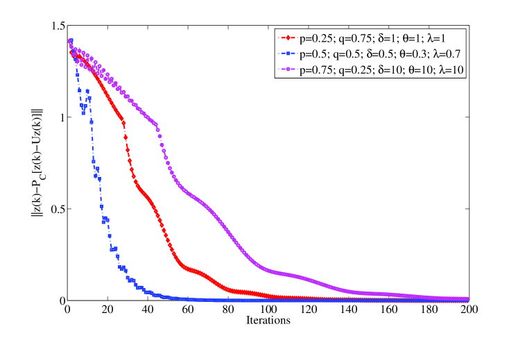
and , for all , where It is easy seen that is paramonotone but is not strictly monotone. We applied Algorithm (2.1) and (2.8) to solve VI().
- •
- •

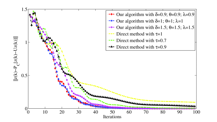
Next, we compare our algorithm (2.8) with the Direct method (Dir.Method) (Algorithm 1 in [8])
| (Dir.Method) |
It was proven in [8] that the trajectory generated by (Dir.Method) converges to an element under the assumption that
| (5.1) |
Due to (5.1), the Dir.Method uses the step sizes , with . In our algorithm, the step size is taken as , where the range of the exponent is wider than of the Dir.Method; in details, . In the numerical examples, we fix and adjust the parameters Let . The comparison are presented in Figure 3. As we can see, in all cases the new algorithm is more efficient than the existing one.
6. Conclusion
We have proposed a second order dynamical system for solving paramonotone VIs in a finite-dimensional space and studied its global convergence. A discretization of this dynamical system gives rise to an inertial iterative projection-type algorithm for which we establish the convergence of the iterations. Some numerical examples are given to confirm the theoretical results and illustrate the effectiveness of the proposed algorithms. The topic for future research includes second order dynamical systems enhanced by the vanishing damping coefficient for solving paramonotone VIs.
Data Availability
Data sets generated during the current study are available from the corresponding author on reasonable request.
Competing interests
The authors declare that they have no competing interests.
References
- [1] B. Abbas, H. Attouch, Benar F. Svaiter: Newton-like dynamics and forward-backward methods for structured monotone inclusions in Hilbert spaces. J. Optim. Theory Appl., 161, 331-360 (2014)
- [2] C.D. Alecsa, S.C. Laszlo, T. Pinta: An Extension of the Second Order Dynamical System that Models Nesterov’s Convex Gradient Method. Appl. Math Optim., 84, 1687-1716 (2021)
- [3] P.K. Anh, N.T. Vinh: Self-adaptive gradient projection algorithms for variational inequalities involving non-Lipschitz continuous operators. Numer. Algorithms, 81, 983-1001 (2019)
- [4] H. Attouch, F. Alvarez: The heavy ball with friction dynamical system for convex constrained minimization problems, in: Optimization (Namur, 1998), Lecture Notes in Economics and Mathematical Systems 481, Springer, Berlin, 25-35, (2000)
- [5] H. Attouch, Z. Chbani, H. Riahi: Combining fast inertial dynamics for convex optimization with Tikhonov regularization. J. Math. Anal. Appl., 457, 1065-1094 (2018)
- [6] H. Attouch, Z. Chbani, H. Riahi: Rate of convergence of the Nesterov accelerated gradient method in the subcritical case . ESAIM, Control Optim. Calc. Var., 25, 1292-8119 (2019)
- [7] T.Q. Bao, P.Q. Khanh: A projection-type algorithm for pseudomonotone nonlipschitzian multi-valued variational inequalities. Nonconvex Optim. Appl., 77, 113-129 (2005)
- [8] J.Y. Bello Cruz, A.N. Iusem: Convergence of direct methods for paramonotone variational inequalities. Comput. Optim. Appl., 46, 247-263 (2010)
- [9] R. I. Bot, E. R. Csetnek: Second order forward-backward dynamical systems for monotone inclusion problems. SIAM J. Control Optim., 54, 1423-1443 (2016)
- [10] R. I. Bot, E. R. Csetnek: Approaching the solving of constrained variational inequalities via penalty term-based dynamical systems. J. Math. Anal. Appl., 435, 1688-1700 (2016)
- [11] Y. Censor, A. Gibali, S. Reich: The subgradient extragradient method for solving variational inequalities in Hilbert space. J. Optim. Theory and Appl., 148, 318-335 (2011)
- [12] E. R. Csetnek: Continuous dynamics related to monotone inclusions and non-smooth optimization problems. Set-Valued Var. Anal., 28(4), 611-642 (2020)
- [13] J.Y. Bello Cruz, R.D. Millán: A direct splitting method for nonsmooth variational inequalities. J. Optim. Theory Appl. 161, 729-737 (2014)
- [14] F. Facchinei, J.-S. Pang: Finite-dimensional variational inequalities and complementarity problems. Springer, New York (2003)
- [15] T.N. Hai: On gradient projection methods for strongly pseudomonotone variational inequalities without Lipschitz continuity. Optim. Lett. 14, 1177-1191 (2020)
- [16] T.N. Hai: Dynamical systems for solving variational inequalities. J. Dyn. Control Syst., 28(4), 681-696, (2022)
- [17] H. Iiduka: Fixed point optimization algorithm and its application to power control in CDMA data networks. Math. Program. 133, 227-242 (2012)
- [18] H. Iiduka, I. Yamada: An ergodic algorithm for the power-control games for CDMA data networks. J. Math. Model. Algorithms 8, 1-18 (2009)
- [19] P.D. Khanh, P.T. Vuong: Modified projection method for strongly pseudomonotone variational inequalities. J. Global Optim. 58, 341-350 (2014)
- [20] D. Kinderlehrer, G. Stampacchia: An introduction to variational inequalities and their applications. Academic Press, New York (1980)
- [21] Y.V. Malitsky, V.V. Semenov: An extragradient algorithm for monotone variational inequalities,. Cybernetics and Systems Anal., 50, 271-277 (2014)
- [22] B.T. Polyak: Some methods of speeding up the convergence of iteration methods. U.S.S.R. Comput. Math. Math. Phys. 4, 1-17 (1964)
- [23] T.D. Quoc, L.D. Muu, V.H. Nguyen: Extragradient algorithms extended to equilibrium problems. Optimization 57, 749-776 (2008)
- [24] M.V. Solodov, B.F. Svaiter: A new projection method for monotone variational inequality problems. SIAM J. Control Optim. 37, 765-776 (1999)
- [25] P.T. Vuong: A second order dynamical system and its discretization for strongly pseudo-monotone variational inequalities. SIAM J. Control Optim., 59(4), 2875-2897 (2021)