VQalAttent: a Transparent Speech Generation Pipeline based on Transformer-learned VQ-VAE Latent Space
Abstract
Generating high-quality speech efficiently remains a key challenge for generative models in speech synthesis. This paper introduces VQalAttent, a lightweight model designed to generate fake speech with tunable performance and interpretability. Leveraging the AudioMNIST dataset, consisting of human utterances of decimal digits (0-9), our method employs a two-step architecture: first, a scalable vector quantized autoencoder (VQ-VAE) that compresses audio spectrograms into discrete latent representations, and second, a decoder-only transformer that learns the probability model of these latents. Trained transformer generates similar latent sequences, convertible to audio spectrograms by the VQ-VAE decoder, from which we generate fake utterances. Interpreting statistical and perceptual quality of the fakes, depending on the dimension and the extrinsic information of the latent space, enables guided improvements in larger, commercial generative models. As a valuable tool for understanding and refining audio synthesis, our results demonstrate VQalAttent’s capacity to generate intelligible speech samples with limited computational resources, while the modularity and transparency of the training pipeline helps easily correlate the analytics with modular modifications, hence providing insights for the more complex models.
Index Terms:
VQ-VAE, neural audio synthesis, decoder-only transformerI Introduction
State-of-the-art generative neural speech synthesis and speech representation learning [1] are usually influenced by the latest AI research in computer vision, which is then adapted and extended leveraging classical speech processing theory and practice. This has been the pattern ever since the first neural synthesis by Wavenet [2]. However, it is the availability of massive computational resources that allowed breakthroughs such as WaveNet or Tacotron 2 [3]. Similar influences exist from Natural Language Processing (NLP) [4], which brought transformers and large language models (LLMs) into the speech synthesis scene [5, 6]. Majority of these neural synthesis models are focused on text-to-speech ([3],[7], [4] and the references therein).
In this paper we introduce and analyze a simple model composed of a learned vector quantizer and a decoder-only transformer. Although of limited scope due to a limited-complexity training dataset, this model allows us to analyze the effects of synthesizing speech in discrete domain, which is enabled by the learned quantization of the latent space of raw acoustic waveforms transformed to spectrograms. Discrete domain synthesis has much lower computational complexity, which creates an opportunity for experimentation and analysis despite the lack of massive computational resources.
Prior Work. WaveNet, a generative neural network introduced by Oord et. al. [2] utilizes dilated convolutions to generate raw waveforms autoregressively. The architecture was based off another autoregressive generative model, PixelCNN, which generated images pixel by pixel. WaveNet model found success with generation of audio data, including speech in various languages and music. While it can generate high fidelity audio and comprehensible speech, the autoregressive method makes WaveNet extremely slow for both training and inference. This is making it inappropriate for use cases that require quick synthesis of audio. Donahue et. al. [8] introduced WaveGAN, a generative adversarial network (GAN) for raw waveform data. In the paper, Donahue et. al. compared the results of WaveGAN against the performance of another GAN model, called SpecGAN. SpecGAN utilizes spectrogram representations of waveforms which are more fitting for machine learning tasks than the waveform representation. The results were interesting, with the SpecGAN-generated samples producing more intelligible results but the WaveGAN generated samples being preferred by human judges. This was likely due to the distortion resulting from the fact that perceptually-informed spectrograms (Mel spectrograms) are not invertible without loss [9]. Similarly, we trained our speech synthesis using a dataset of spectrograms, and we observed the same audio artifacts when the synthesized data is played back. However, this is of no importance here, as the play-back quality could be improved by utilizing invertible transforms or by a post-hoc vocoder, while the statistical properties of the generated samples in the spectrogram domain showed desired similarity with the originals. HuBERT [10], a very popular approach to learning self-supervised speech representations for speech recognition, generation, and compression, was one of the first models that used clusterization to discretize the space of speech signals. Other models use AI discrete codecs to learn a well-discretized latent space and then train an autoregressive model in that discrete space [1]. This alleviates the computational latency problem, inherent to autoregressive approaches. There are multiple models that leverage the ability of VQ-VAE [11] to learn discrete latent representations [12], which are particularly useful for capturing the complex structures present in audio data.
Hence, the type of approach that we are using is not novel, but other models that leverage VQ-VAE for discretization are overly complex, with diverse components and multi-modal loss functions, which makes the analysis very difficult. For example, [6] utilizes multiple quantization codebooks for variable bandwidth in the end-to-end training of the model pipeline which consists of a transformer, a GAN architecture, an arithmetic encoder and several loss components, including multiple reconstruction losses and an adversarial loss mechanized by the GAN. As the speech synthesis in discrete domain is fairly new, we believe that VQalAttent, the model with a straightforward architecture proposed here, will contribute to better understanding of this approach. The main contribution of this architecture is the model transparency, allowing for a scalable model adaptation, followed by the comparative analysis based both on tracking the shift in learned probability distribution and on assessing classification accuracy. Adaptations demonstrated here include dimensionality of discrete representations (compression ratio), codebook initialization, conditional generation with the condition prompt embedded in the discrete representation sequence, and the choice of the transformer model.
II System Model
Our methodology involves two models. We use a vector-quantizing auto-encoder (VQ-AE), which is typically referred to as VQ-VAE, despite the fact that it is not trained using variational inference. For this reason, we will also use the acronym VQ-VAE, since the architecture that we are using allows for variational inference using a Kullback-Liebler (KL) distance between the uniform probability mass function of discretized data and the learned posterior probability mass function. We use VQ-VAE to learn discrete latent representations of the audio recordings in AudioMNIST, converted to spectrograms. The training involves choosing a discretization model that has the most perceptible reconstructions since the quality of the reconstructions reflect the quality of the learned representation. Using these learned discrete latents, we train an autoregressive model to learn the prior over the latents representing the training dataset. The particular model that we use is a decoder-only-transformer with self-attention blocks, each with heads. Through autoregressive sampling of the trained transformer, we generate deep fakes. In the absence of human judges to score the intelligibility of our deep fakes, we will use the accuracy score of a deep classifier to determine how perceptible the reconstructed samples are (Table I). We will also measure the shift in learned probability distribution with respect to original data by characterizing the overlapping between the original and the fake manifolds using metrics such as fidelity (coverage) and diversity.
II-A Vector Quantized Variational Autoencoder
Vector Quantized Variational Autoencoder (VQ-VAE) [11] is an autoencoder which learns a discrete latent representation of the input data, in contrast to the continuous latent space learning in standard variational and non-variational autoencoders. The encoder, denoted , transforms the input data into a sequence of latent vectors of length . These latent vectors are then discretized by applying a quantization function , which maps each latent vector to an element of a learnable codebook consisting of learnable embedding vectors of the same length . The decoder block, denoted , is tasked with reconstructing the original input from the mapped codebook vectors. While the most intuitive and most common choice for is to simply perform a nearest neighbor lookup, more advanced techniques such as stochastic codeword selection [13] or heuristics such as exponential moving averages (EMA) [14] can be employed instead. We utilized both. The 3 elements of the VQ-VAE architecture are shown in Fig. 1 and the forward path through VQ-VAE is given by Equation (1) in which is the latent representation of at the output of while is its quantized version. We introduce another form of the quantized latent , denoted in Fig. 1 by which replaces the codewords quantizing the s vectors with their indices in the codebook. We refer to those indices as tokens
| (1) |
More rigorously, the indexed (discrete) is obtained as
| (2) |
where the expectation depends on the quantization algorithm is the th codeword of the codebook and is the th slice (vector) of the latent tensor of length equal to the length of In Fig. 1, the token’s index goes from to which is how many vectors of length the tensor consists of, for a specific compression rate (to be referred as the Case 2 VQ-VAE).
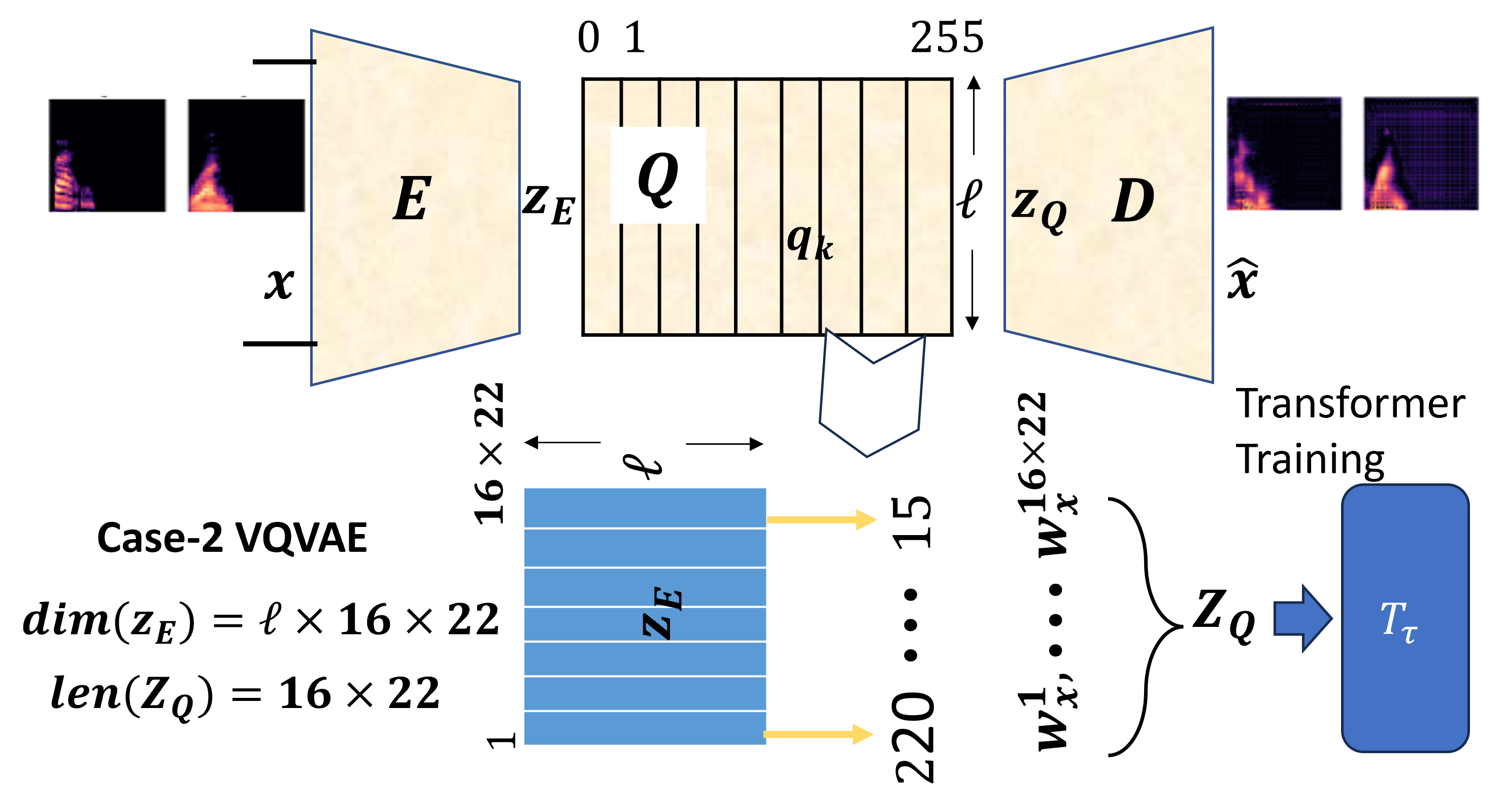
The architecture of the encoder is composed of 3 convolutional layers and 3 residual blocks, while the decoder has an equivalent symmetric architecture. The VQ-VAE, whose loss function is composed of a reconstruction loss and a latent quantization loss (commitment cost) , is trained for 100 epochs. For , we include a KL loss between and a uniform prior. Note that the VQ-VAE trainable parameters are represented in Equation (1) as and denoting Encoder’s weights, Codebook trainable codewords and Decoder’s weights, respectively.
II-B Decoder-Only Transformer
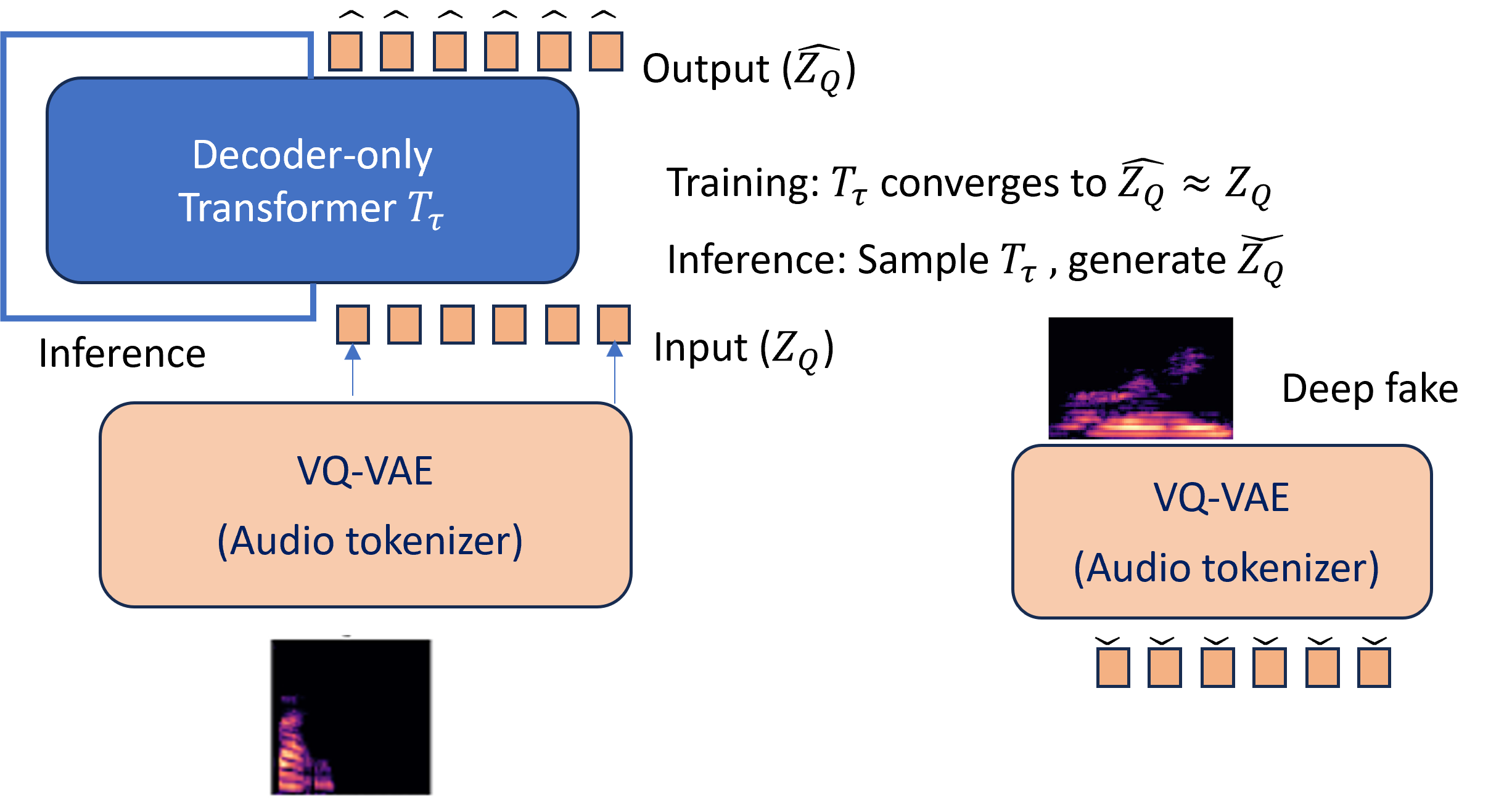
The Decoder-only Transformer model [15], also known as the autoregressive Transformer, is a variation of the original encoder-decoder transformer model proposed by Vaswani et. al. [16]. This model omits the encoder stack, utilizing only the decoder stack to learn the causal attention structure in and to perform autoregressive sequence generation, once trained. The model’s self-attention mechanism enables the model to predict the next token in a sequence by attending to all previous tokens. It also allows for the use of cross-attention, but does not specify how the cross-attending context is obtained (as opposed to an encoder-decoder architecture where the cross-attention context is coming from the encoder). As illustrated in Fig. 2, during the training of the transformer, the masked indexed output of the VQ-VAE quantizer is compared with its estimate at the output of the transformer using a cross-entropy loss. At the inference, we start from a random token, and continue generating subsequent tokens of a fake auto-regressively. We convert (2) into its non-indexed version and feed it into the VQ-VAE decoder to generate the spectrogram of the discrete latent deep fake produced by the transformer.
III Methodology
In this section, we outline how our model is parameterized and trained, and how we design experiments to explore the following questions:
-
•
Can our model generate coherent, comprehensible human speech samples?
-
•
Can the model be extended to conditionally generate speech based on content (e.g., digit labels) and speaker characteristics (e.g., gender)?
-
•
How the model adaptation affects the above aspects?
III-A Data
We use the AudioMNIST dataset, consisting of labeled, short audio samples of spoken numerals (0-9) [17]. The dataset uses a variety of speakers of different ethnicities and genders.
We opt for a spectrogram representation, a visualization of the signal frequency spectrum over time. Specifically, we will use the Mel-spectrogram. The Mel-spectrogram converts frequencies to Mel scale which is meant to approximate humans’ non-linear frequency response, i.e., our greater sensitivity to changes in low frequencies. Our complete data preprocessing pipeline is as follows:
-
1.
Resample audio recordings to 22,050 Hz.
-
2.
Trim the leading and trailing silence, where 15dB under the peak amplitude is considered silence.
-
3.
Fix the length of sampled recordings to a fixed duration by performing a time stretch.
-
4.
Apply the Mel-spectrogram transformation to obtain spectrograms as images of size , with the number of gray pixels totaling per spectrogram.
-
5.
Convert spectrogram values from linear-scale to decibels.
-
6.
Apply min-max normalization.
We refer to the training dataset composed of such spectrograms as Similarly, test dataset is referred to as
III-B Training
We utilize a two-stage training procedure: first, we train the VQ-VAE model, followed by the training of the autoregressive transformer in Fig. 2.
As described in Section II, in the initial training stage the VQ-VAE model will learn the discrete embeddings to achieve an efficient, discretized representation of the input data, which can be reconstructed by the VQ-VAE decoder into speech utterances perceptually resembling the originals. This is the non-generative part. Such discrete ordinal data is well-suited for our transformer model with minimal preprocessing. The model is then trained on the latent sequences of tokens representing datapoints in our training set. We train 2 versions of this 2-stage pipeline: 1) , which has longer token sequences due to a VQ-VAE encoder dimensioned to compress the spectrograms with compression ratio , from the original , to dimensions (ordinal tokens); 2) , which produces shorter token sequences due to compression ratio , from the original , to dimensions (ordinal tokens).
Dimensioning of the VQ-VAE/ transformer pipeline is determined by the desired dimension of the latent tensor which was guided by the following experiment: we performed a PCA decomposition of and counted the number of components whose explained variance constitute 99% of the total variance. This number determined the dimension of in Case 1 (which is close, while easily implemented), while Case 2 was obtained by decreasing the second and third dimension of the encoder’s output by half. Hence is expected to reconstruct the data with high fidelity if properly trained.
Learning the posterior. In a Bayesian treatment we imply that latent variables govern the distribution of the data. Hence, looking at VQalAttent via a Bayesian model, we want to generate deep fakes by drawing latent variables from a prior distribution and then relate them to the observations through the likelihood implemented by the VQVAE decoder. However, with the quantization step in VQ-VAE, we trained a discrete transform that maps the latents into discrete latents . More precisely, we learned a posterior by training the VQ-VAE with spectrograms , whose parametric model is expressed by Eqn. (1).
Learning the prior. To sample from our codebook, allowing generation of new (fake) samples, we must learn the prior of our discrete latent sequences generated from
We will learn probability model by training the transformer to learn its autoregressive form .
After applying based on a trained codebook of to an input , we get a sequence of integers The same processed by results in We generate such sequences for each resulting in 2 datasets and for training 2 versions of the transformer. It should be noted that is a representation of obtained using the encoder of which generates it from the non-ordinal version of Thus we simplify our problem of generating deep fakes from generative models trained directly on spectrograms of real valued features by training generative models and in the discrete latent space using and of dimension and respectively.
Once we learn the prior as a joint autoregressive distribution of ordered tokens after training on the datasets and , we can feed a randomly chosen value for into the respective transformer model and have the model predict the next values, with and respectively. We then perform the procedure explained above to construct our spectrogram from the generated indices.
Autoregressive Models. Our choice for the autoregressive model is a decoder-only transformer [15] (see also Subsection II-B). More specifically, we modify an open-source implementation [18] of the decoder-only-transformer. Every transformer model uses a process called multi-headed self-attention to learn the context and relationships between the tokens which are the comprising elements of training sequences. The hyperparameters of the VQalAttent transformer are the vocabulary size, which is the amount of unique input tokens, equal to and the context size which represents the number of tokens in the latent sequence that the model is able to process at a time. For two different values of based on two different VQ-VAE compression ratios, we train two different transformers and In addition to and referred to as unconditioned transformers, we also train and by modifying datasets and so that the sequences of tokens are extended by the class token. The class token is obtained from the label of the original used to produce matching sequences This is an innovative way of introducing the extrinsic context in the decoder-only transformer, without creating an embedding for it. Sampling the trained and allows us to obtain deep fakes for which we know the label (digit ). This will be used to assess the quality of the fakes by evaluating the accuracy of their classification on a pretrained classifier (Fig. 3). We next analyze the performance of VQalAttent as a function of and selected hyperparameters.
IV Evaluation
Establishing a quantitative metric for evaluating the effectiveness of a generative model at generating deepfakes is a topic being actively discussed and researched. In this section, we discuss some of the metrics applied to evaluate both the unconditionally and the conditionally trained generative models. Some methods only work for the conditionally generated samples since we know the class of the fakes being generated, based on the class token.
After training the conditioned transformer for each label equally, we created one dataset of fakes per label by sampling the model autoregressively, starting from the label token Each set represents learned conditional prior distribution . We put all those fakes together into one conditional dataset and create another dataset of original discrete latents of the same size and label distribution. We will use these datasets to evaluate the quality of fake latents generated by the conditioned transformers.
By autoregressively sampling the two unconditioned models and starting from the uninformative token only, we create two datasets of unconditioned fakes of the same size as .
IV-A Classifier
To score the perceptual clarity of the VQ-VAE reconstructions in the absence of human judges, and to quantify the success of our conditional generative models in generating the perceptible fakes, we evaluate the accuracy score achieved by a deep classifier on the reconstructions and on the conditionally generated data derived from , respectively. Not having the ground truth label for the fakes generated by the unconditioned transformer, we omit this type of evaluation for The classifier was trained on the original data preprocessed as described. The architecture used is of our own design and was tuned to give maximum accuracy on the test set of original data (100%). The classifier’s architecture is described in Fig. 3.
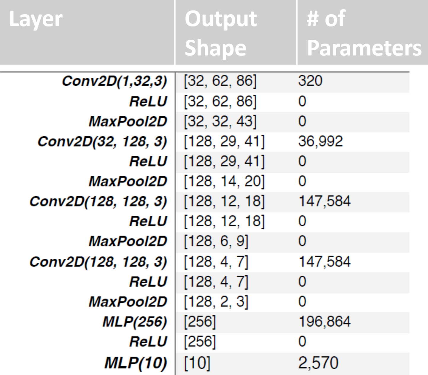
The classifier-based evaluation outputs the accuracy of the VQ-VAE reconstructions per compression case (1 for lower and 2 for higher compression), and for the respective fakes. It is presented in Table I, where VQ-VAE reconstructions are marked with letter and the spectrograms generated from the latent fakes produced by the transformer are marked by where for case 1 and 2, respectively.
| R case 1 | R case 2 | |||
|---|---|---|---|---|
| Accuracy | 0.966 | 0.961 | 0.912 | 0.909 |
All the accuracy results in Table I are lower than the accuracy obtained for the original spectrograms, which suggests that the pipeline should have been trained for longer time. We currently train each VQ-VAE model for 100 epochs and each transformer for 50 epochs, which is a strain on our computational resources, given the number of model variants. However, the differences among tested datasets are logical, in that lower compression performs better than the higher compression.
IV-B Quantitative evaluation using fidelity and diversity
A generative model should try to achieve good trade-off between 1. fidelity (how realistic each fake is) and 2. diversity (how well fake samples capture the variations in real samples). We here present the evaluation of both the conditioned and unconditioned generations using the metrics which capture those two aspects in a statistically consistent manner. Fidelity is related to the precision measure, which expresses probability that a random fake falls into the support of the real datapoints, while the diversity resembles the recall measure, a probability that a random real sample falls into the support of the fakes [19]. The key word here is the support. The evaluation based on fidelity and diversity defines the support as based only on the statistically relevant samples.
The Topological Precision and Recall (TopP&R, pronounced ’topper’), [20] provides a systematic approach to estimating supports of the original and generated data, retaining only topologically and statistically important features with a certain level of confidence. This allows TopP&R to stay relevant for noisy features, and provides statistical consistency. Hence, the widespread metrics of precision and recall, applied on the topologically significant features, are called fidelity and diversity, and used to express relevant qualities in the context of generative sampling.
Diversity (Recall) counts significant real samples on the fake manifold, expressing the ability to find all relevant instances of every class and variety in the learned data distribution. Fidelity (Precision) counts significant fake samples on the real manifold, expressing the typicality of the fakes. High number of ”hallucinations” would decrease this score. Confidence band for significant samples and the manifolds are estimated using Kernel Density Estimator (KDE) [20]. Let us denote the relevant fake instances from a randomly generated set of fakes by indicating that these instances fall withing the real manifold. Similarly, the set collects random real instances from the test set which fall withing the fake manifold.
Looking at the TopP&R results in Table II, we observe that the diversity is outstanding across the evaluated pipelines. As we evaluated the model with the fastest training first, we encountered the TopP&R results from the conditioned transformer first: fidelity: 0.904, diversity: 0.986, Top F1: 0.943. We suspected that the diversity is outstanding because we trained conditioned transformers to learn conditional joint distributions of tokens for each label separately, and then sampled each of those distributions by starting from the class token. In other words, we obtained good diversity because we forced it by sampling an equal number of samples from each class token. Next, we evaluated the matching unconditioned transformer , which learned the unconditioned prior Using the fakes generated by , we obtained somewhat surprising TopP&R results (table II): the diversity stayed outstanding, but the fidelity went down. By listening to generated fakes, we identified every single digit class and a good variety of male and female voices, which explains high diversity. However, some of the digits were unintelligible due to the noise induced by inverting Mel spectrogram. The fact that some fakes can be clearly identified by human listeners despite the loss due to inversion, indicates that there are good quality fakes that are fairly resilient to the inversion loss. However, those that are unintelligible probably contributed to the drop in fidelity. For the and the fidelity further decreased, which we assumed is the consequence of the artifacts due to insufficient training, given that longer token sequences require longer training. In fact, the current Top P%R values for and are obtained by increasing the training to 70 epochs, since the 50 epochs resulted in fidelity close to zero. Please see the table II which displays unconditioned and conditioned TopP&R values together.
| Fidelity | 0.51 | 0.45 | 0.57 | 0.90 |
| Diversity | 1.0 | 1.0 | 1.0 | 0.99 |
| TopF1 | 0.68 | 0.62 | 0.72 | 0.94 |
We also hypothesize that training the unconditioned transformers longer, or with a more complex transformer architecture, can decrease the gap in Table II. This is because the embedding of the class label in the training sequence decreases the uncertainty in the training data, allowing the transformer model to be easily trained, while the opposite is true for unconditioned sequences of tokens.
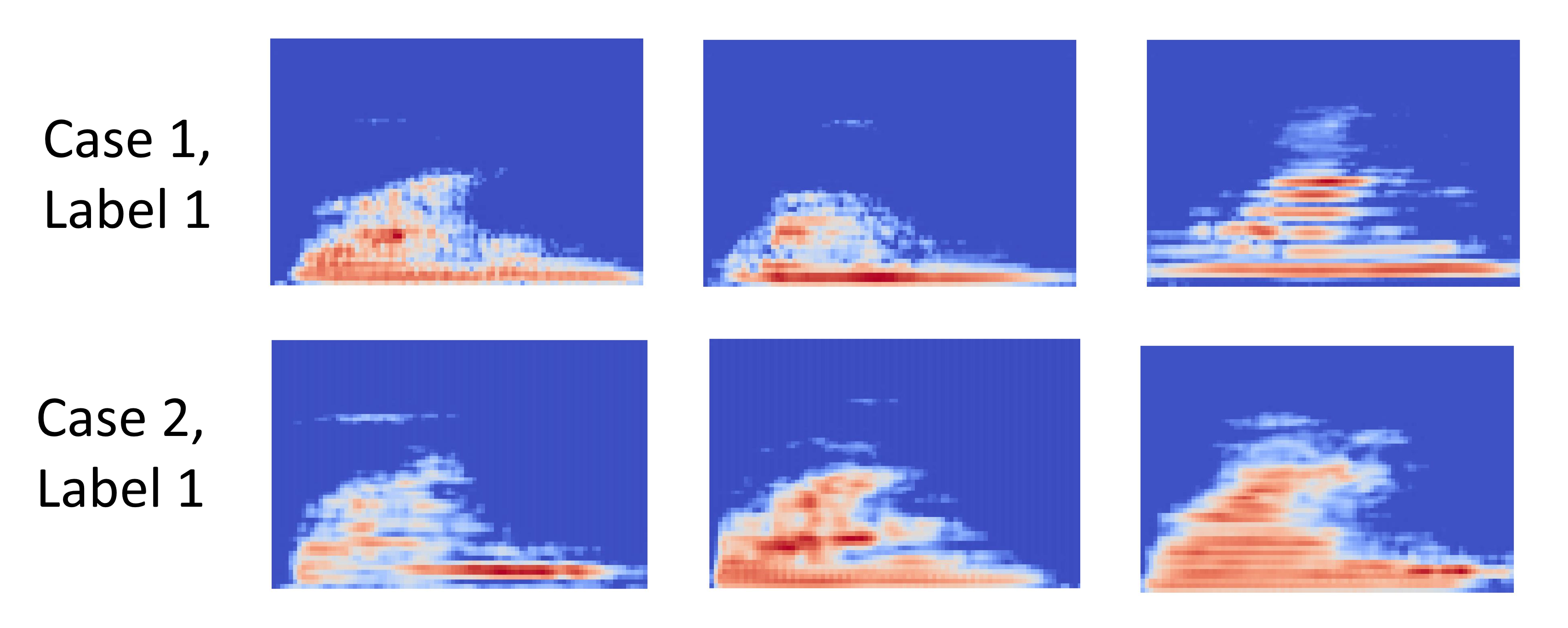
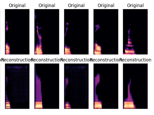
IV-C Qualitative
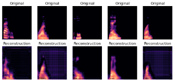
Fig. 4 demonstrates how difficult it is to evaluate quality of the fakes, even if they are generated conditionally, for a single class. This is due to the diversity of genders and accents present in the training data. Hence, if properly trained, the transformer will generate very diverse voices, both male and female, and with different accents and annunciation, even if the numeral class is constrained. Inspecting only a few spectrograms (Fig. 4), or playing back a few waveforms derived from such spectrograms is only a practical tool, which can be used to track improvements in the training based on the subjective sense of clarity. Visually comparing originals with VQ-VAE reconstructions in Fig. 5 and even with conditionally generated spectrograms can demonstrate some artifacts due to compression, but any probability shift in the generated fakes (learned distribution) is impossible to detect via visual inspection.
V Conclusion
We analyzed a two-stage pipeline of a generative model trained to produce deep fakes of spoken numerals. The pipeline consists of 1) a VQ-VAE which discretizes latent representations of the spectrograms obtained from the AudioMNIST dataset, and 2) a decoder-only transformer which is trained to learn the prior of discretized latents. We trained 2 versions of 2 differently dimensioned pipelines, one version conditioned on the class label matching the spoken numeral’s latent, and another where the label was not presented in the training data. Dimensioning of the VQ-VAE/ transformer pipeline was determined by the desired dimension of the latent tensor explicitly related to the information reduction ratio. We evaluated all mentioned generative models using diverse metrics, including fidelity, diversity and class recognition, and analyzed the impacts of compression, discretization in the latent space, presence of the label-based context and model architectures. Future works includes a more rigorous analysis of the architectural effects, additional training, and the inclusion of diverse data and data transforms in the original and latent space. It will be informed by the dependencies revealed by the VQalAttent analysis, thanks to the simplicity, transparency and modularity of our approach.
References
- [1] A. Mohamed, H.-y. Lee, L. Borgholt, J. D. Havtorn, J. Edin, C. Igel, K. Kirchhoff, S.-W. Li, K. Livescu, L. Maaløe et al., “Self-supervised speech representation learning: A review,” IEEE Journal of Selected Topics in Signal Processing, vol. 16, no. 6, 2022.
- [2] A. v. d. Oord, S. Dieleman, H. Zen, K. Simonyan, O. Vinyals, A. Graves, N. Kalchbrenner, A. Senior, and K. Kavukcuoglu, “Wavenet: A generative model for raw audio,” arXiv preprint arXiv:1609.03499, 2016.
- [3] J. Shen, R. Pang, R. J. Weiss, M. Schuster, N. Jaitly, Z. Yang, Z. Chen, Y. Zhang, Y. Wang, R. Skerrv-Ryan et al., “Natural tts synthesis by conditioning wavenet on mel spectrogram predictions,” in 2018 IEEE international conference on acoustics, speech and signal processing (ICASSP). IEEE, 2018, pp. 4779–4783.
- [4] H. Wu, X. Chen, Y.-C. Lin, K.-w. Chang, H.-L. Chung, A. H. Liu, and H.-y. Lee, “Towards audio language modeling-an overview,” arXiv preprint arXiv:2402.13236, 2024.
- [5] Wen-Chin Huang et al., “Pretraining techniques for sequence-to-sequence voice conversion,” IEEE/ACM Trans. on Audio, Speech, and Language Processing, vol. 29, 2021.
- [6] A. Défossez, J. Copet, G. Synnaeve, and Y. Adi, “High fidelity neural audio compression,” arXiv preprint arXiv:2210.13438, 2022.
- [7] S. Chen, S. Liu, L. Zhou, Y. Liu, X. Tan, J. Li, S. Zhao, Y. Qian, and F. Wei, “Vall-e 2: Neural codec language models are human parity zero-shot text to speech synthesizers,” 2024.
- [8] C. Donahue, J. McAuley, and M. Puckette, “Adversarial audio synthesis,” arXiv preprint arXiv:1802.04208, 2018.
- [9] D. Griffin and J. Lim, “Signal estimation from modified short-time fourier transform,” IEEE Transactions on Acoustics, Speech, and Signal Processing, 1984.
- [10] W.-N. Hsu, B. Bolte, Y.-H. H. Tsai, K. Lakhotia, R. Salakhutdinov, and A. Mohamed, “Hubert: Self-supervised speech representation learning by masked prediction of hidden units,” IEEE/ACM Transactions on Audio, Speech, and Language Processing, vol. 29, pp. 3451–3460, 2021.
- [11] A. Van Den Oord, O. Vinyals et al., “Neural discrete representation learning,” Advances in neural information processing systems, vol. 30, 2017.
- [12] P. Dhariwal, H. Jun, C. Payne, J. W. Kim, A. Radford, and I. Sutskever, “Jukebox: A generative model for music,” arXiv preprint arXiv:2005.00341, 2020.
- [13] C. K. Sonderby, B. Poole, and A. Mnih, “Continuous Relaxation Training of Discrete Latent Variable Image Models,” in Intern. Conf. on Neural Information Processing Systems, 2017.
- [14] A. Razavi, A. van den Oord, and O. Vinyals, “Generating diverse high-fidelity images with VQ-VAE-2,” in Intern. Conf. on Neural Information Processing Systems, 2019.
- [15] A. Radford, K. Narasimhan, T. Salimans, and I. Sutskever, “Improving language understanding by generative pre-training,” https://cdn.openai.com/research-covers/ language-unsupervised/language_understanding_paper.pdf, 2018.
- [16] A. Vaswani, N. Shazeer, N. Parmar, J. Uszkoreit, L. Jones, A. N. Gomez, Ł. Kaiser, and I. Polosukhin, “Attention is all you need,” Advances in neural information processing systems, vol. 30, 2017.
- [17] S. Becker, J. Vielhaben, M. Ackermann, K.-R. Müller, S. Lapuschkin, and W. Samek, “AudioMNIST: Exploring Explainable Artificial Intelligence for audio analysis on a simple benchmark,” Journal of the Franklin Institute, vol. 361, no. 1, 2024.
- [18] Walter H. L et al., “Generative AI for Medical Imaging: extending the MONAI Framework,” 2023. [Online]. Available: https://arxiv.org/abs/2307.15208
- [19] M. S. e. a. Sajjadi, “Assessing generative models via precision and recall,” Advances in neural information processing systems, 2018.
- [20] P. J. Kim, Y. Jang, J. Kim, and J. Yoo, “Toppr: Robust support estimation approach for evaluating fidelity and diversity in generative models,” arXiv preprint arXiv:2306.08013, 2023.