Modelling Loss of Complexity in Intermittent Time Series and its Application

Abstract

In this paper, we developed a nonparametric relative entropy (RlEn) for modelling loss of complexity in intermittent time series. This technique consists of two steps. First, we carry out a nonlinear autoregressive model where the lag order is determined by a Bayesian Information Criterion (BIC), and complexity of each intermittent time series is obtained by our novel relative entropy. Second, change-points in complexity were detected by using the cumulative sum (CUSUM) based method. Using simulations and compared to the popular method appropriate entropy (ApEN), the performance of RlEn was assessed for its (1) ability to localise complexity change-points in intermittent time series; (2) ability to faithfully estimate underlying nonlinear models. The performance of the proposal was then examined in a real analysis of fatigue-induced changes in the complexity of human motor outputs. The results demonstrated that the proposed method outperformed the ApEn in accurately detecting complexity changes in intermittent time series segments.

Keywords— Intermittent time series, change-point detection, relative entropy, transformation invariant, background-noise-free

1 Introduction

Intermittent time series is widely recorded in various fields, such as neurological examination (Burioka et al., 2005), heart rate analysis (Acharya U et al., 2004), sports science (Forrest et al., 2014) and energy demand (Li et al., 2024). The intermittent time series contains the information of various patterns or models. For instance, in Magnetoencephalography (MEG) or Electroencephalogram (EEG) scan, neurologically healthy subjects respond differently in terms of EEG and MEG signal for different stimuli (faces v.s. scrambled faces, or familiar faces v.s. unfamiliar faces, see Wakeman and Henson (2015)); In cardiology, the pattern of heart rate varies along the states of human: sleeping, sitting, walking, jogging or running, see Acharya U. et al. (2005), Burioka et al. (2005), Shi et al. (2017) and among others; In sports science, the energy offered by Adenosine triphosphate (ATP) will gradually reduce along the time, the torque shows different models, see Figures 1(a) and 2(a). Scientists have a great interested in detecting the change-points among a consecutive intermittent time series to help scientists to identify the patterns of brain activity, the heart disease or improve the performance of athlete.

Throughout this research, the terminology change-point refers to the “change-point” among intermittent time series rather than the “change-point” within a specific time series. The usual change-points are the break points within one piece of time series, see Killick et al. (2012); Fryzlewicz (2014); Li et al. (2024). However, the change-points in this article are the break points among the intermittent time series. For example, suppose we have extracted 55 intermittent time series from Figure 1(a). Sports scientists want to know the time of muscle fatigue occurrence. In this case, the time of muscle fatigue occurrence is one type of change-point among intermittent time series.

To identify the change-points among a consecutive intermittent time series using cumulative summation (CUSUM) based method (Page, 1954; Killick et al., 2012; Fryzlewicz, 2014; Wang and Samworth, 2017), it is necessary to map each intermittent time series to a scalar. Subsequently, a CUSUM-based method can be applied to the resulting series of scalars. Let $\mathbbm{x}_{t}=(x_{t1},\ldots,x_{tN})$ be a univariate intermittent time series with length $N$ where $t$ represents the time. $T$ is the number of intermittent isometric time series. Then $\mathbbm{x}_{1},\mathbbm{x}_{2},\ldots,\mathbbm{x}_{T}$ represent a consecutive intermittent isometric time series. Denote the map function as $\mathcal{I}:\mathbb{R}^{N}\mapsto\mathbb{R}$. Mathematically, the change-point detection among intermittent isometric time series is equivalent to the change-points detection of $\{\mathcal{I}(\mathbbm{x}_{1}),\mathcal{I}(\mathbbm{x}_{2}),\ldots,\mathcal{I}(\mathbbm{x}_{T})\}$. In particular, if $N=1$ and $\mathcal{I}(\cdot)$ is an identify function, the problem of detecting change-point among intermittent time series degenerates to the classical change-point detection problem.

For the choice of map function $\mathcal{I}(\cdot)$, we require it owns the following two properties: transformation invariant and background-noise-free. The transformation invariant property means that $\mathcal{I}(\mathbbm{x}_{t})$ equals $\mathcal{I}(h(\mathbbm{x}_{t}))$ where $h(\mathbbm{x}_{t})$ is a sufficient statistics of $\mathbbm{x}_{t}$. Let the noise of $\mathbbm{x}_{t},t=1,2,\ldots,T$ follow normal distribution with zero mean and variance $\sigma^{2}$. The background-noise-free property means that the result of map function $\mathcal{I}(\cdot)$ should be free from $\sigma^{2}$. The former property could eliminate the impact of unit while the latter property guarantees that the $\mathcal{I}(\cdot)$ does not include the variance of background noise. Table 1 summarises five potential choices of $\mathcal{I}(\cdot)$: mean, variance, entropy (En), conditional entropy (CoEn) and relative entropy (RlEn) and their properties.

	Mean	Variance	En	CoEn	RlEn
Transformation invariant	✘	✘	✘	✘	✔
Background-noise-free	✔	✘	✘	✘	✔

Table 1: Potential choices of $\mathcal{I}(\cdot)$ and their properties. En, CoEn and RlEn represent entropy, conditional entropy and relative entropy respectively.

1. Mean and Variance. Suppose $\mathcal{I}(\cdot)$ represents mean function, $\mathbbm{y}_{t}=h(\mathbbm{x}_{t})=\alpha\mathbbm{x}_{t}$ is a linear transformation, $\alpha\neq 0$. Then $\bar{\mathbbm{y}}_{t}$ = $\alpha\bar{\mathbbm{x}}_{t}\neq\bar{\mathbbm{x}}_{t}$. If $\mathbbm{x}_{t}$ is independent of $\sigma^{2}$, then for any transformation $h(\cdot)$, $h(\mathbbm{x}_{t})$ is also independent of $\sigma^{2}$. Similarly, one can easily verify that variance does not have these two properties.

2. Entropy (En) and Conditional Entropy (CoEn). Entropy and conditional entropy are inappropriate choice of $\mathcal{I}(\cdot)$ because:

• Entropy is scale variant, for example, let $\text{En}(x)$ represent the entropy of variable $x$, for any scale transformation $y=\alpha x$, $\alpha\in\mathbb{R}$ and $\alpha\neq 0$ then the entropy of variable $y$ is $\text{En}(x)+\log\left|\alpha\right|$. More generally, entropy is not transformation invariant under change of variable as well, see Ihara (1993, p.18).

• Conditional entropy is neither transformation invariant. In nonparametric settings, the four entropies: Approximate Entropy (ApEn) (Pincus, 1991), Sample Entropy (SpEn) (Richman and Moorman, 2000), Multi-scale Entropy (MsEn) (Costa et al., 2003) and Fuzzy Entropy (FzEn) (Chen et al., 2009) are the special cases of conditional entropy. They do not own the property of transformation invariant. For instance, when one uses the multivariate uniform kernel to estimate the nonparametric CoEn, the difference between ApEn and CoEn is $\log(2h)$ which comes from the scale transformation in kernel function with bandwidth $h$.

• Besides, entropy and conditional entropy are not background-noise-free. A direct example can be found in Appendix A. Equations (22) and (23) are entropy and conditional entropy respectively, however both are related to the $\sigma^{2}$.

3. Relative Entropy (RlEn). Kullback and Leibler (1951) have proved that RlEn has the property of transformation invariant. The discussion of background-noise-free property is put off in Propositions B.1 in Appendix.

In this article, we will use the relative entropy (RlEn) as the map function for $\mathbbm{x}_{t}$. Relative entropy is also called Kullback-Leibler divergence (Kullback and Leibler, 1951). It is a measure to describe the divergence between two probability distributions. Robinson (1991) proposed a consistent nonparametric entropy-based test for independence in time series which employed the sample splitting device. To avoid the hyperparameter for the sample splitting device, Hong and White (2005) developed an asymptotic distribution theory for nonparametric entropy of serial dependence. Unlike Hong and White (2005) had obtained an asymptotic distribution of relative entropy for pairwise variables, we proposed the relative entropy for $m$-consecutive variables in high-dimensional context where $m\geq 2$. Furthermore, we recommand using the BIC criterion to select the pre-determined parameter $m$. The consistency theory of BIC is developed to ensure that the estimator of lag order converges to the true order with probability 1. Under certain assumptions, the limiting distribution of nonparametric RlEn is Gaussian with convergence rate $\sqrt{n}h^{(m+1)/2}$.

This article is organized as follows. In Section 2, we introduce the methodology of relative entropy for $m$-consecutive variables, the BIC criterion to select the optimal lag order as well as the algorithms. In Section 3, we derive the asymptotic distribution of relative entropy. In Section 4, we provide simulation studies to illustrate the performance of the proposed method, and we apply the proposed method to the real data set in Section 5. Finally, we conclude the article in Section 6.

2 Methodology

Let $X_{1},\ldots,X_{N}$ represent the time-varying scalar measurements, which form a strictly stationary process. Denote $\mathbf{X}_{i;m}={(X_{i},\ldots,X_{i+m-1})}^{\top}$ as the $m$ consecutive variables vector where $m$ could be sufficiently large but be bounded by $M$. The density function of $\mathbf{X}_{i;m}$ is defined as $g(\mathbf{X}_{i;m})$. Furthermore, let $\mathbf{X}_{i;m+1}={(X_{i},\ldots,X_{i+m})}^{\top}$ and $f(\mathbf{X}_{i;m+1})$ be the $m+1$ consecutive variables vector and its probability density function. Note that given the first vector $\mathbf{X}_{i;m}$, the conditional probability density function of $X_{i+m}$ is $f(X_{i+m}\mid\mathbf{X}_{i;m})=f(\mathbf{X}_{i;m+1})/g(\mathbf{X}_{i;m})$. Furthermore, let $g_{1}(X_{i+m})$ be the density function of $X_{i+m}$, then the relative entropy is defined as

$$\mathfrak{E}\coloneqq\mathbb{E}_{f}\left[\log\left(\frac{f\left(\mathbf{X}_{i;m+1}\right)}{g\left(\mathbf{X}_{i;m}\right)g_{1}(X_{i+m})}\right)\right],$$

where $\mathbb{E}_{f}$ represent the expectation with resepect to the density funciton $f$. In mathematical statistics, $\mathfrak{E}$ is also called Kullback–Leibler (KL) divergence (Kullback and Leibler, 1951). Estimation of $\mathfrak{E}$ can be divided into two parts: the density estimation and expectation estimation.

For density estimation, we use nonparametric kernel method to estimate $f(\mathbf{X}_{i;m+1})$, $g(\mathbf{X}_{i;m})$ and $g_{1}(X_{i+m})$. Jackknife kernel has been proposed to mitigate the boundaries effect for the kernel with bounded support (John, 1984; Härdle, 1990; Jones, 1993). Additionally, other popular methods in the literature address boundary effects in kernel density estimation, such as the reflection method (Schuster, 1985), the transformation method (Marron and Ruppert, 1994), and local polynomial density estimation (Chen, 1999). Researchers can choose to use these alternative methods but must adapt the theory presented in Section 3. For consistency, we employ the Jackknife kernel to estimate the densities in this section.

Following John (1984), we suppose Assumption 2.1 holds throughout this article.

Assumption 2.1.

The domain of kernel function $K(\cdot)$ is $[-1,1]$ and $K(\cdot)$ satisfies $K(-x)=K(x)$ for any $x\in[-1,1]$, $\int_{-1}^{+1}K(x)\,\mathrm{d}x=1$ and $\int_{-1}^{+1}x^{2}K(x)\,\mathrm{d}x<+\infty$.

In fact, the Jackknife kernel is a linear combination of two different self-normalized kernel, namely,

$$k_{\rho}(u)=(1+\beta(\rho))\frac{K(u)}{\omega_{0}(\rho)}-\frac{\beta(\rho)}{\alpha}\frac{K(u/\alpha)}{\omega_{0}(\rho/\alpha)},$$

where $\omega_{l}(\rho)=\int_{-1}^{\rho}u^{l}K(u)\,\mathrm{d}u$, $l=0,1,2$, $0\leq\rho\leq 1$ and $\beta(\rho)=\frac{R_{1}(\rho)}{\alpha R_{1}(\rho/\alpha)-R_{1}(\rho)}$, where $R_{l}(\rho)=\omega_{l}(\rho)/\omega_{0}(\rho)$, $l=1,2$. In this article, we follow the choice of $\alpha$ in John (1984) and let $\alpha=2-\rho$. Finally, for univariate $x,y\in[0,1]$, the Jackknife kernel is defined as

$$K_{h}^{J}(x-y)\coloneqq\begin{cases}h^{-1}k_{(x/h)}\left(\frac{x-y}{h}\right),&\text{if}\,x\in[0,h).\\ h^{-1}K\left(\frac{x-y}{h}\right),&\text{if}\,x\in[h,1-h].\\ h^{-1}k_{[(1-x)/h]}\left(\frac{x-y}{h}\right),&\text{if}\,x\in(1-h,1].\end{cases}$$

For more details of Jackknife kernel, see John (1984) and Hong and White (2005). For vectors $\mathbf{x}=(x_{1},\ldots,x_{m})$ and $\mathbf{y}=(y_{1},\ldots,y_{m})$, we define the scaled multivariate Jackknife kernel as

$$\mathcal{K}^{(m)}_{h}(\textbf{x}-\textbf{y})\coloneqq K_{h}^{J}(x_{1}-y_{1})\times K_{h}^{J}(x_{2}-y_{2})\times\cdots\times K_{h}^{J}(x_{m}-y_{m}).$$ (1)

Following the assumption in Hong and White (2005), we assume the bandwidths for each component of $x_{1},\ldots,x_{m}$ in equation (1) are same, i.e., $h$.

Let $x_{1},\ldots,x_{N}$ be the observations of $X_{1},\ldots,X_{N}$, $\mathbf{x}_{i;m}$ and $\mathbf{x}_{i;m+1}$, $i=1,\ldots,N-m$ are the corresponding observations of $\mathbf{X}_{i;m}$ and $\mathbf{X}_{i;m+1}$, respectively. From now on, we define $n\coloneqq N-m$ to simplify the notations in this paper. The “leave-one-out” kernel density estimators of $f(\cdot),g(\cdot)$ and $g_{1}(\cdot)$ are:

$$\hat{f}\left(\mathbf{x}_{i;m+1}\right) =\frac{1}{n-1}\sum\nolimits_{j=1}^{n}\mathcal{K}^{(m+1)}_{h}\left(\mathbf{x}_{i;m+1}-\mathbf{x}_{j;m+1}\right)\mathbbm{1}(j\neq i),$$

$$\hat{g}\left(\mathbf{x}_{i;m}\right) =\frac{1}{n-1}\sum\nolimits_{j=1}^{n}\mathcal{K}^{(m)}_{h}\left(\mathbf{x}_{i;m}-\mathbf{x}_{j;m}\right)\mathbbm{1}(j\neq i),$$

$$\hat{g}_{1}(x_{i+m}) =\frac{1}{n-1}\sum\nolimits_{j=1}^{n}K_{h}^{J}(x_{i+m}-x_{j+m})\mathbbm{1}(j\neq i),$$

where $i,j\in\{1,2,\ldots,n\}$ and $\mathbbm{1}(\cdot)$ is the indicator function. Then, the nonparametric estimator of $\mathfrak{E}$ can be expressed as

$$\hat{\mathfrak{E}}(m,h|\mathfrak{X})=\frac{1}{n}\sum_{i\in S(m)}\log\frac{\hat{f}\left(\mathbf{x}_{i;m+1}\right)}{\hat{g}\left(\mathbf{x}_{i;m}\right)\hat{g}_{1}(x_{i+m})},$$ (2)

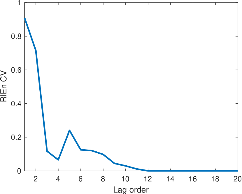
(a) $h=0.05$

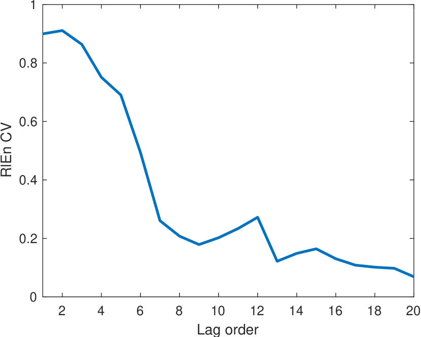
(b) $h=0.1$

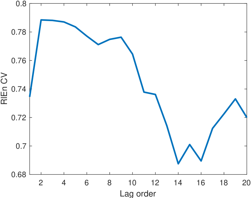
(c) $h=0.2$

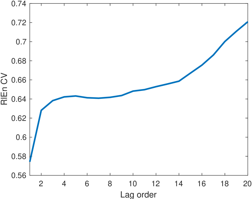
(d) $h=0.3$

Figure 5: Relative Entropy against Lag Order for Different Bandwidths

where $S(m)=\{i\in\mathbb{N}:1\leq i\leq n,\hat{f}(\mathbf{x}_{i;m+1})>0,\hat{g}(\mathbf{x}_{i;m})>0,\hat{g}_{1}(x_{i+m})>0\}$ and $\mathfrak{X}=\{x_{1},x_{2},\ldots,x_{N}\}$. We observe that the estimator $\hat{\mathfrak{E}}(m,h|\mathfrak{X})$ depends on the unknown lag order $m$ and bandwidth $h$. In practice, one can either (a) estimate $m$ first and then estimate the bandwidth $h$; or (b) estimate the bandwidth $h$ first and then estimate $m$. However, given $h$, maximizing the estimator (2) with respect to $m$ is not an appropriate criterion for selecting $m$, as the curve of $\hat{\mathfrak{E}}(m,h|\mathfrak{X})$ against $m$ varies significantly for different bandwidths (see Figure 5). In practice, our suggestion is to determine the lag order $m$ prior to computing the relative entropy $\hat{\mathfrak{E}}(m,h|\mathfrak{X})$. Then, for the specified $\hat{m}$, we select the bandwidth by maximizing the estimator (2), i.e,

$$\hat{h}=\operatorname*{arg\,max}_{h}\hat{\mathfrak{E}}(\hat{m},h|\mathfrak{X}).$$

In the next section, we use BIC criterion to select the optimal lag order $\hat{m}$ based on the general nonlinear autoregression model.

2.1 Lag Order Selection

The general nonlinear autoregression model studied in this circumstance is

$$x_{i+m}=\mathfrak{F}\left(\mathbf{x}_{i;m}\right)+\varepsilon_{i},$$ (3)

where $1\leq m\leq N-1$, $\varepsilon_{i}$ is Gaussian white noise with zero mean and variance $\sigma^{2}$. $\mathfrak{F}(\cdot)$ is an unknown function. The Nadaraya-Watson estimator of $\mathfrak{F}(\mathbf{x}_{i;m})$ can be expressed as:

$$\hat{\mathfrak{F}}\left(\mathbf{x}_{i;m},h_{*}\right)=\sum\nolimits_{j=1}^{n}l_{j}\left(\mathbf{x}_{i;m},h_{*}\right)x_{j+m},\quad i=1,2,\ldots,n$$ (4)

where

$$l_{j}\left(\mathbf{x}_{i;m},h_{*}\right)=\frac{\mathcal{K}_{h_{*}}^{(m)}\left(\mathbf{x}_{j;m}-\mathbf{x}_{i;m}\right)}{\sum_{s=1}^{n}\mathcal{K}_{h_{*}}^{(m)}\left(\mathbf{x}_{s;m}-\mathbf{x}_{i;m}\right)},\quad j=1,\ldots,n.$$

$h_{*}$ is the bandwidth for nonlinear autoregression model. Denote $L(h_{*})$ as

$$L(h_{*})\coloneqq\begin{bmatrix}l_{1}\left(\mathbf{x}_{1;m},h_{*}\right)&l_{2}\left(\mathbf{x}_{1;m},h_{*}\right)&\cdots&l_{n}\left(\mathbf{x}_{1;m},h_{*}\right)\\ l_{1}\left(\mathbf{x}_{2;m},h_{*}\right)&l_{2}\left(\mathbf{x}_{2;m},h_{*}\right)&\cdots&l_{n}\left(\mathbf{x}_{2;m},h_{*}\right)\\ \vdots&\vdots&\cdots&\vdots\\ l_{1}\left(\mathbf{x}_{n;m},h_{*}\right)&l_{2}\left(\mathbf{x}_{n;m},h_{*}\right)&\cdots&l_{n}\left(\mathbf{x}_{n;m},h_{*}\right)\\ \end{bmatrix}.$$ (5)

Then we have the following Lemma.

Lemma 2.1.

For the multivariate kernel $\mathcal{K}_{h_{*}}^{(m)}(\cdot)$ and Nadaraya-Watson estimator (4), $L(h_{*})$ is defined in (5), the effective degrees of freedom $v$ has explicit expression as

$$v(m,h_{*})=\text{{tr}}(L(h_{*}))=\mathcal{K}_{h_{*}}^{(m)}\left(\mathbf{0}\right)\sum\nolimits_{i=1}^{n}{\left(\sum\nolimits_{s=1}^{n}\mathcal{K}_{h_{*}}^{(m)}\left(\mathbf{x}_{s;m}-\mathbf{x}_{i;m}\right)\right)}^{-1}=O(h_{*}^{-m}).$$

The proof is straightforward which will be omitted here. The bandwidth is selected by so-called leave-one-out cross validation method, i.e., minimizing

$$\hat{h}_{*}(m)=\operatorname*{arg\,min}_{h_{*}}\sum\nolimits_{i=1}^{n}{\left(x_{i+m}-\hat{\mathfrak{F}}_{-i}\left(\mathbf{x}_{i;m},h_{*}\right)\right)}^{2},$$

where

$$\hat{\mathfrak{F}}_{-i}\left(\mathbf{x}_{i;m},h_{*}\right)=\sum_{j=1}^{n}\frac{\mathcal{K}_{h_{*}}^{(m)}\left(\mathbf{x}_{j;m}-\mathbf{x}_{i;m}\right)}{\sum_{s=1,s\neq i}^{n}\mathcal{K}_{h_{*}}^{(m)}\left(\mathbf{x}_{s;m}-\mathbf{x}_{i;m}\right)}x_{j+m}.$$

Define the average square predict error as

$$\hat{\sigma}^{2}(m)=\frac{1}{n}\sum\nolimits_{i=1}^{n}{\left(x_{i+m}-\hat{\mathfrak{F}}_{-i}\left(\mathbf{x}_{i;m},\hat{h}_{*}(m)\right)\right)}^{2},$$

then, we have the following BIC criterion

$$\mathfrak{B}(m)=n\log(\hat{\sigma}^{2}(m))+v(m,\hat{h}_{*}(m))\log(n),\quad m=1,2,\ldots,N-1.$$ (6)

Immediately, we have

Theorem 2.2.

Supposing $m_{0}\in\{1,2,\ldots,N-1\}$ be the underlying lag order. Let $\hat{m}=\operatorname*{arg\,min}_{m}\mathfrak{B}(m)$. Under conditions (C1)–(C7) in Appendix C of Appendix, $\hat{m}$ converges to $m_{0}$ in probability, i.e.,

$$P(\hat{m}=m_{0})\rightarrow 1.$$

The proof details of Theorem 2.2 can be found in Appendix C of Appendix. There exist various criteria proposed to address the lag order selection problem (Shibata, 1981; Vieu, 1995; Shao, 1997). This proof follows the framework of Vieu (1995) combining the discussion in Shao (1997). We can use criterion (6) to choose $m$ in advance, then implement the computation of relative entropy.

2.2 Change-points Detection

In the previous subsection, we have discussed the relative entropy of a time series segment for ARMA processes and nonparametric settings. Similarly, we can apply the same procedure to the other time series segments. Once we obtain the relative entropies of time series segments, denoted as $\mathfrak{E}_{1},\mathfrak{E}_{2},\ldots,\mathfrak{E}_{J}$ where $J$ represents the number of time series segments. Then, we can apply the existing detection methods such as CUSUM (Page, 1954) and its variants (Inclán and Tiao, 1994; Picard et al., 2011), quasi-likelihood (Braun et al., 2000). In this chapter, we employ the proposed detection method (Killick et al., 2012) to search the change-points as they pointed out that the optimal change-points can be detected with a linear computational cost. Furthermore, their method has been officially adopted in the function findchangepts by MATLAB since 2018, which is convenient in the context of our algorithms below.

2.3 Algorithms

In practice, let $\mathcal{X}={(x_{ij})}_{N\times J}$. Each column of $\mathcal{X}$ represents a time series with length $N$. Suppose $\mathcal{X}$ has been transformed by the following logistic function,

$$\mathcal{X}=\frac{1}{1+\exp\left(-\mathcal{Y}\right)},$$ (7)

where $\mathcal{Y}$ represents the original time series observations without bounded support. Similar to Hong and White (2005), we use the logistic function (7) to ensure the compact support in 3.1 throughout this chapter.

Finally, we summarize our approach using the following two algorithms:

Data: Matrix observation $\mathcal{X}$ with size $N\times J$.

Result: $\hat{m}$, the optimal lag order of $\mathcal{X}$.

Init: $M\leftarrow 10$

1 for $j\leftarrow 1$ to $J$ do

2       $m_{j}\leftarrow 0$

3       $\mathcal{X}_{j}\leftarrow\mathcal{X}(:,j)$

4       for $m\leftarrow 1$ to $M$ do

5             $n\leftarrow N-m$

6             for $i\leftarrow 1$ to $n$ do

7                   $\mathbf{x}_{i;m}\leftarrow\mathcal{X}_{j}(i:(i+m-1))$

8                   $x_{i+m}\leftarrow\mathcal{X}_{j}(i+m)$

9                  

10             end for

11            $h_{*}\leftarrow\operatorname*{arg\,min}_{h_{*}}1/n\sum_{i=1}^{n}{\left(x_{i+m}-\hat{g}_{-i}\left(\mathbf{x}_{i;m},h_{*}\right)\right)}^{2}$

12             $v(m,h_{*})\leftarrow\text{{tr}}(L(h_{*}))$

13             $\hat{\sigma}^{2}\leftarrow 1/n\sum_{i=1}^{n}{\left(x_{i+m}-\hat{g}\left(\mathbf{x}_{i;m},h_{*}\right)\right)}^{2}$

14             $\mathfrak{B}_{j}(m)\leftarrow n\log(\hat{\sigma}^{2})+v(m,h_{*})\log(n)$

15            

16       end for

17      

18 end for

19$\overline{\mathfrak{B}}(m)=J^{-1}\sum_{j=1}^{J}\mathfrak{B}_{j}(m)$

20 $\hat{m}\leftarrow\operatorname*{arg\,min}_{m}\{\overline{\mathfrak{B}}(m),m=1,\ldots,M\}$

Algorithm 1 M step

Data: Matrix observation $\mathcal{X}$ with size $N\times J$.

Result: $\hat{j}$, the change-points.

Init: $\hat{m}$ from Algorithm 1

1 for $j\leftarrow 1$ to $J$ do

2       $\mathfrak{E}_{j}\leftarrow 0$

3       $\mathcal{X}_{j}\leftarrow\mathcal{X}(:,j)$

4       $\hat{h}\leftarrow\operatorname*{arg\,min}_{h}\left\{\hat{\mathfrak{E}}(\hat{m},h|\mathcal{X}_{j})\right\}$ (Estimator (2))

5       $\mathfrak{E}_{j}\leftarrow\hat{\mathfrak{E}}(\hat{m},\hat{h}|\mathcal{X}_{j})$

6      

7 end for

8$\hat{j}\leftarrow$ change point detected from $\mathfrak{E}_{j},j=1,\ldots,J$ using the proposed method (Killick et al., 2012)

Algorithm 2 E Step

In Algorithm 1, one can specify the initial value of $M$. We take 10 as the default value following the suggestion from Section 4.5 in Wasserman (2006). The bandwidth selection consumes most computation time. To reduce the time of selection $h_{*}$, one can choose $h_{*}$ moderately at the order $O(n^{-1/(4+m)})$ as an initial value, see Section 8.2 in Fan and Yao (2003) for more details.

In Algorithm 2, we implement the bandwidth selection as well. The main difference is that the Algorithm 1 includes the multivariate nonparametric regression but in Algorithm 2, $\mathfrak{E}$ includes the multivariate nonparametric kernel density estimation.

3 Theory

Hong and White (2005) have proved that the relative entropy of pairwise variable $(X_{t},X_{t-j})$ has a normal limiting distribution. The basic idea of Hong and White (2005)’s proof is to decompose the relative entropy into some different items, then expand each item to different parts by neglecting the smaller ones. Heuristically, the main parts can be expressed by the U-statistics. By discussing the limiting distribution of these U-statistics, they finally established consistency theory of relative entropy for pairwise variables.

In this section, we develop a consistency theory of the relative entropy for $m$ consecutive variables. By using their proving skills and ideas, we show that the limiting distribution of consecutive variable is Gaussian as well if $m$ has an upper bound, say $M$. The framework of our proof is very similar to that of Hong and White (2005)’s proof. Hence, the notations and most Lemmas and Theorems below originate from the theory and Appendix in Hong and White (2005). However, our theory is not a straightforward extension from pairwise variables to $m$ consecutive variable. There are some key points that need to be emphasized in our theory because they are different from those in Hong and White (2005)’s proof. In the following Theorems, Lemmas as well as their proofs in Appendix D, we will highlight these key points where they need to be emphasized.

From now on, we abbreviate $\hat{\mathfrak{E}}(m,h|\mathfrak{X})$ as $\hat{\mathfrak{E}}(m)$. Next we rewrite the estimator (2), namely

$$\hat{\mathfrak{E}}(m) =\frac{1}{n}\sum_{i\in S(m)}\left\{\log\left[\frac{f\left(\mathbf{x}_{i;m+1}\right)}{g\left(\mathbf{x}_{i;m}\right)g_{1}(x_{i+m})}\right]+\log\left[\frac{\hat{f}\left(\mathbf{x}_{i;m+1}\right)}{f\left(\mathbf{x}_{i;m+1}\right)}\right]\right.$$ (8)

$$\qquad-\left.\log\left[\frac{\hat{g}\left(\mathbf{x}_{i;m}\right)}{g\left(\mathbf{x}_{i;m}\right)}\right]-\log\left[\frac{\hat{g}_{1}(x_{i+m})}{g_{1}(x_{i+m})}\right]\right\},$$

$$=\hat{I}_{m}(f,g\cdot g_{1})+\hat{I}_{m}(\hat{f},f)-\hat{I}_{m}(\hat{g},g)-\hat{I}_{1}(\hat{g}_{1},g_{1}).$$

Under the following null hypothesis:

$$\mathbb{H}_{0}:f\left(\mathbf{x}_{i;m+1}\right)=g\left(\mathbf{x}_{i;m}\right)g_{1}(X_{i+m}),$$

the first term in equation (8), $\hat{I}_{m}(f,g\cdot g_{1})=0$ almost surely. Note that for $\left|x\right|<1$, we have the inequality $\left|\log(1+x)-x+\frac{1}{2}x^{2}\right|\leq{\left|x\right|}^{3}$, so the third term in equation (8) can be expressed as

$$\hat{I}_{m}(\hat{g},g) =\frac{1}{n}\sum_{i\in S(m)}\log\left[1+\frac{\hat{g}\left(\mathbf{x}_{i;m}\right)-g\left(\mathbf{x}_{i;m}\right)}{g\left(\mathbf{x}_{i;m}\right)}\right],$$ (9)

$$=\frac{1}{n}\sum_{i=1}^{n}\left[\frac{\hat{g}\left(\mathbf{x}_{i;m}\right)-g\left(\mathbf{x}_{i;m}\right)}{g\left(\mathbf{x}_{i;m}\right)}\right]$$

$$\qquad-\frac{1}{2}\sum_{i=1}^{n}{\left[\frac{\hat{g}\left(\mathbf{x}_{i;m}\right)-g\left(\mathbf{x}_{i;m}\right)}{g\left(\mathbf{x}_{i;m}\right)}\right]}^{2}+\text{remainder},$$

$$=\hat{W}_{1}(m)-\frac{1}{2}\hat{W}_{2}(m)+\text{remainder}.$$

To obtain the consistency results of (9), we need the following assumption.

Assumption 3.1.

Suppose $\{X_{t}\}$ is strictly stationary time series with the support $\mathbb{I}=[0,1]$. Let $\mathcal{G}:\mathbb{I}\rightarrow\mathbb{R}^{+}$ be the marginal density of $X_{t}$. On support $\mathbb{I}$, $\mathcal{G}$ is away from 0 and has twice continuously differentiation $\mathcal{G}^{(2)}(\cdot)$. Furthermore, $\mathcal{G}^{(2)}(\cdot)$ satisfies the Lipschitz condition, i.e., for any $x_{1},x_{2}\in\mathbb{I}$, $\left|\mathcal{G}^{(2)}(x_{1})-\mathcal{G}^{(2)}(x_{2})\right|\leq\mathcal{L}\left|x_{1}-x_{2}\right|$, where $\mathcal{L}$ is the Lipschitz constant.

Moreover, at the bounds 0 and 1, the first and second derivatives of $\mathcal{G}(\cdot)$ are defined by their right-hand derivative and left-hand derivative respectively. Assumption 3.1 is quite general and can avoid the slower convergence rate at the bounds of $\mathbb{I}$ (Hall, 1988; Robinson, 1991; Hong and White, 2005).

To expand the term $\hat{W}_{1}(m)$, we need to introduce some notations: for any vector $\mathbf{z}_{1},\mathbf{z}_{2}\in\mathbb{I}^{m}$, define $\bar{g}(\mathbf{z}_{1})=\int_{\mathbb{I}^{m}}\mathcal{K}^{(m)}_{h}(\mathbf{z}_{1},\mathbf{z}_{2})g(\mathbf{z}_{2})d\mathbf{z}_{2}$, where $\mathcal{K}^{(m)}_{h}(\mathbf{z}_{1},\mathbf{z}_{2})=\mathcal{K}^{(m)}_{h}(\mathbf{z}_{1}-\mathbf{z}_{2})$. Let

$$\tilde{\mathcal{K}}_{h}^{(m)}(\mathbf{z}_{1},\mathbf{z}_{2})=\mathcal{K}^{(m)}_{h}(\mathbf{z}_{1},\mathbf{z}_{2})-\int_{\mathbb{I}^{m}}\mathcal{K}^{(m)}_{h}(\mathbf{z},\mathbf{z}_{2})d\mathbf{z},$$

$$\tilde{A}_{m}(\mathbf{z}_{1},\mathbf{z}_{2})=\left[\tilde{\mathcal{K}}_{h}^{(m)}(\mathbf{z}_{1},\mathbf{z}_{2})-\int_{\mathbb{I}^{m}}\tilde{\mathcal{K}}_{h}^{(m)}(\mathbf{z}_{1},\mathbf{z})g(\mathbf{z})d\mathbf{z}\right]/g(\mathbf{z}_{1}),$$

$$A_{m}(\mathbf{z}_{1},\mathbf{z}_{2})=\left[\mathcal{K}_{h}^{(m)}(\mathbf{z}_{1},\mathbf{z}_{2})-\int_{\mathbb{I}^{m}}\mathcal{K}_{h}^{(m)}(\mathbf{z}_{1},\mathbf{z})g(\mathbf{z})d\mathbf{z}\right]/g(\mathbf{z}_{1}),$$ (10)

$$\gamma_{m}(\mathbf{z}_{1},\mathbf{z}_{2})=\int_{\mathbb{I}^{m}}\left[\mathcal{K}_{h}^{(m)}(\mathbf{z},\mathbf{z}_{2})-\int_{\mathbb{I}^{m}}\mathcal{K}_{h}^{(m)}(\mathbf{z},\mathbf{z}^{*})g(\mathbf{z}^{*})d\mathbf{z}^{*}\right]d\mathbf{z}/g(\mathbf{z}_{1}),$$

$$B_{m}(\mathbf{z}_{1})=\left[\int_{\mathbb{I}^{m}}\mathcal{K}_{h}^{(m)}(\mathbf{z}_{1},\mathbf{z})g(\mathbf{z})d\mathbf{z}-g(\mathbf{z}_{1})\right]/g(\mathbf{z}_{1}),$$

$$H_{1m}(\mathbf{z}_{1},\mathbf{z}_{2})=\tilde{A}_{m}(\mathbf{z}_{1},\mathbf{z}_{2})+\tilde{A}_{m}(\mathbf{z}_{2},\mathbf{z}_{1}),$$ (11)

$$H_{2m}(\mathbf{z}_{1},\mathbf{z}_{2})=\int_{\mathbb{I}^{m}}A_{m}(\mathbf{z},\mathbf{z}_{1})A_{m}(\mathbf{z},\mathbf{z}_{2})g(\mathbf{z})\,\mathrm{d}\mathbf{z},$$

$$\hat{C}(m)=\frac{1}{n}\sum\nolimits_{i=1}^{n}\int_{\mathbf{z}\in\mathbb{I}^{m}}A_{m}\left(\mathbf{z},\mathbf{x}_{i;m}\right)B_{m}(\mathbf{z})g(\mathbf{z})\,\mathrm{d}\mathbf{z},$$ (12)

then, we have

$$\hat{W}_{1}(m) =\frac{1}{2}\binom{n}{2}^{-1}\sum_{j=2}^{n}\sum_{i=1}^{j-1}\left[\tilde{A}_{m}\left(\mathbf{x}_{i;m},\mathbf{x}_{j;m}\right)+\tilde{A}_{m}\left(\mathbf{x}_{j;m},\mathbf{x}_{i;m}\right)\right]$$ (13)

$$\qquad+\frac{1}{2}\binom{n}{2}^{-1}\sum_{j=2}^{n}\sum_{i=1}^{j-1}\left[\gamma_{m}\left(\mathbf{x}_{i;m},\mathbf{x}_{j;m}\right)+\gamma_{m}\left(\mathbf{x}_{j;m},\mathbf{x}_{i;m}\right)\right]$$

$$\qquad+\frac{1}{n}\sum_{i=1}^{n}B_{m}\left(\mathbf{x}_{i;m}\right),$$

$$=\frac{1}{2}\hat{H}_{1}(m)+\frac{1}{2}\hat{\Gamma}(m)+\hat{B}(m).$$

Next, we discuss the expansion of second term in equation (9). We write

$$\hat{W}_{2}(m) =\hat{W}_{21}(m)+\hat{W}_{22}(m)+\hat{W}_{23}(m),$$ (14)

where

$$\hat{W}_{21}(m)=n^{-1}\sum\nolimits_{i=1}^{n}{\left[\left(\hat{g}\left(\mathbf{x}_{i;m}\right)-\bar{g}\left(\mathbf{x}_{i;m}\right)\right)\big{/}g\left(\mathbf{x}_{i;m}\right)\right]}^{2},$$

$$\hat{W}_{22}(m)=n^{-1}\sum\nolimits_{i=1}^{n}{\left[\left(\bar{g}\left(\mathbf{x}_{i;m}\right)-g\left(\mathbf{x}_{i;m}\right)\right)\big{/}g\left(\mathbf{x}_{i;m}\right)\right]}^{2},$$

and

$$\hat{W}_{23}(m)=\frac{2}{n}\sum_{i=1}^{n}\left[\frac{\hat{g}\left(\mathbf{x}_{i;m}\right)-\bar{g}\left(\mathbf{x}_{i;m}\right)}{g\left(\mathbf{x}_{i;m}\right)}\right]\left[\frac{\bar{g}\left(\mathbf{x}_{i;m}\right)-g\left(\mathbf{x}_{i;m}\right)}{g\left(\mathbf{x}_{i;m}\right)}\right].$$

Let $D_{m}(\mathbf{z}_{1},\mathbf{z}_{2})=A_{m}^{2}(\mathbf{z}_{1},\mathbf{z}_{2})+A_{m}^{2}(\mathbf{z}_{2},\mathbf{z}_{1})$ and

$$\tilde{H}_{2m}(\mathbf{z}_{1},\mathbf{z}_{2},\mathbf{z}_{3}) =A_{m}(\mathbf{z}_{1},\mathbf{z}_{2})A_{m}(\mathbf{z}_{1},\mathbf{z}_{3})+A_{m}(\mathbf{z}_{2},\mathbf{z}_{3})A_{m}(\mathbf{z}_{2},\mathbf{z}_{1})$$

$$\qquad+A_{m}(\mathbf{z}_{3},\mathbf{z}_{1})A_{m}(\mathbf{z}_{3},\mathbf{z}_{2}),$$

then after some simple calculations, we can obtain

$$\hat{W}_{21}(m)=\frac{1}{2(n-1)}\hat{D}(m)+\frac{1}{3}\frac{n-2}{n-1}\tilde{H}_{2}(m),$$ (15)

where $\hat{D}(m)=\binom{n}{2}^{-1}\sum_{j=2}^{n}\sum_{i=1}^{j-1}D_{m}(\mathbf{x}_{i;m},\mathbf{x}_{j;m})$ and

$$\tilde{H}_{2}(m)=\binom{n}{3}^{-1}\sum_{k=3}^{n}\sum_{j=2}^{k-1}\sum_{i=1}^{j-1}\tilde{H}_{2m}(\mathbf{x}_{k;m},\mathbf{x}_{i;m},\mathbf{x}_{j;m}).$$

The remainder term in Equation 9 has the order of $O_{p}\left(n^{-3/2}h^{-3m/2}{(\log{n})}^{1/2}+m^{2}h^{6}\right)$ (see Lemma D.1) Combining Equations (9), (13), (14) and (15), we finally have

$$\hat{I}_{m}(\hat{g},g) =\frac{1}{2}\hat{H}_{1}(m)+\frac{1}{2}\hat{\Gamma}(m)+\hat{B}(m)-\frac{1}{4(n-1)}\hat{D}(m)$$ (16)

$$\qquad-\frac{n-2}{6(n-1)}\tilde{H}_{2}(m)-\frac{1}{2}\hat{W}_{22}(m)-\frac{1}{2}\hat{W}_{23}(m)$$

$$\qquad+O_{p}\left(\frac{{(\log{n})}^{1/2}}{n^{3/2}h^{3m/2}}+m^{2}h^{6}\right).$$

In Appendix D, Lemmas D.2, D.3, D.4, D.5 and D.6 give the orders of terms $\hat{\Gamma}(m)$, $\hat{D}(m)$, $\tilde{H}_{2}(m)$, $\hat{W}_{22}(m)$ and $\hat{W}_{23}(m)$ in Equation 16 respectively. Based on these theory results, we immediately have Theorem 3.1.

Theorem 3.1.

Given Assumptions 2.1 and 3.1, if $2\leq m<M$, $nh^{m}\rightarrow\infty$, $nh^{m+12}\rightarrow 0$ and ${(\log n)}^{1/2}/(nh^{m})\rightarrow 0$, then under $\mathbb{H}_{0}$,

$$\hat{I}_{m}(\hat{g},g)=\frac{1}{2}\hat{H}(m)-\frac{1}{2}L(m)+\left[\hat{B}(m)-\hat{C}(m)\right]+o_{p}(n^{-1/2}h^{-m/2}),$$

where $\hat{H}(m)=\hat{H}_{1}(m)-(n-2)/(n-1)\hat{H}_{2}(m)$, $L(m)={(n-1)}^{-1}\mathbb{E}A^{2}_{m}(\mathbf{z}_{1},\mathbf{z}_{2})+\mathbb{E}B_{m}^{2}(\mathbf{z}_{1})$, $\mathbf{z}_{1},\mathbf{z}_{2}\in\mathbb{I}^{m}$ and $\mathbf{z}_{1},\mathbf{z}_{2}$ have no overlap variable,

$$\hat{H}_{1}(m) =\binom{n}{2}^{-1}\sum\nolimits_{j=2}^{n}\sum\nolimits_{i=1}^{j-1}H_{1m}\left(\mathbf{x}_{i;m},\mathbf{x}_{j;m}\right),$$

$$\hat{H}_{2}(m) =\binom{n}{2}^{-1}\sum\nolimits_{j=2}^{n}\sum\nolimits_{i=1}^{j-1}H_{2m}\left(\mathbf{x}_{i;m},\mathbf{x}_{j;m}\right).$$

The proof of Theorem 3.1 is straightforward which we omit here. Similarly, we can obtain the corresponding results with $g(\cdot)$ being replaced by $g_{1}(\cdot)$ and $f(\cdot)$ respectively. Specifically, we have the following two theorems.

Theorem 3.2.

Given Assumptions 2.1 and 3.1, if $nh^{m+1}\rightarrow\infty$, ${(\log n)}^{1/2}/(nh^{m+1})\rightarrow 0$, $nh^{m+13}\rightarrow 0$ and $1\leq m<M$, for any vector $\mathbf{z}_{1},\mathbf{z}_{2}\in\mathbb{I}^{m+1}$, define

$$\bar{f}(\mathbf{z}_{1})=\int_{\mathbb{I}^{m+1}}\mathcal{K}^{(m+1)}_{h}(\mathbf{z}_{1},\mathbf{z}_{2})f(\mathbf{z}_{2})d\mathbf{z}_{2},$$

where $\mathcal{K}^{(m+1)}_{h}(\mathbf{z}_{1},\mathbf{z}_{2})=\mathcal{K}^{(m+1)}_{h}(\mathbf{z}_{1}-\mathbf{z}_{2})$. Let

$$\tilde{K}_{h}^{J}(\mathbf{z}_{1},\mathbf{z}_{2})=\mathcal{K}^{(m+1)}_{h}(\mathbf{z}_{1},\mathbf{z}_{2})-\int_{\mathbb{I}^{m+1}}\mathcal{K}^{(m+1)}_{h}(\mathbf{z},\mathbf{z}_{2})d\mathbf{z},$$

$$\tilde{A}_{(m+1)}(\mathbf{z}_{1},\mathbf{z}_{2})=\left[\tilde{K}_{h}^{J}(\mathbf{z}_{1},\mathbf{z}_{2})-\int_{\mathbb{I}^{m+1}}\tilde{K}_{h}^{J}(\mathbf{z}_{1},\mathbf{z})f(\mathbf{z})d\mathbf{z}\right]/f(\mathbf{z}_{1}),$$

$$A_{(m+1)}(\mathbf{z}_{1},\mathbf{z}_{2})=\left[\mathcal{K}_{h}^{(m+1)}(\mathbf{z}_{1},\mathbf{z}_{2})-\int_{\mathbb{I}^{m+1}}\mathcal{K}_{h}^{(m+1)}(\mathbf{z}_{1},\mathbf{z})f(\mathbf{z})d\mathbf{z}\right]/f(\mathbf{z}_{1}),$$

$$\gamma_{(m+1)}(\mathbf{z}_{1},\mathbf{z}_{2})=\int_{\mathbb{I}^{m+1}}\left[\mathcal{K}_{h}^{(m+1)}(\mathbf{z},\mathbf{z}_{2})-\int_{\mathbb{I}^{m+1}}\mathcal{K}_{h}^{(m+1)}(\mathbf{z},\mathbf{z}^{*})f(\mathbf{z}^{*})d\mathbf{z}^{*}\right]d\mathbf{z}/f(\mathbf{z}_{1}),$$

$$B_{(m+1)}(\mathbf{z}_{1})=\left[\int_{\mathbb{I}^{m+1}}\mathcal{K}_{h}^{(m+1)}(\mathbf{z}_{1},\mathbf{z})f(\mathbf{z})d\mathbf{z}-f(\mathbf{z}_{1})\right]/f(\mathbf{z}_{1}),$$

$$H_{1(m+1)}(\mathbf{z}_{1},\mathbf{z}_{2})=\tilde{A}_{(m+1)}(\mathbf{z}_{1},\mathbf{z}_{2})+\tilde{A}_{(m+1)}(\mathbf{z}_{2},\mathbf{z}_{1}),$$

$$H_{2(m+1)}(\mathbf{z}_{1},\mathbf{z}_{2})=\int_{\mathbb{I}^{m+1}}A_{(m+1)}(\mathbf{z},\mathbf{z}_{1})A_{(m+1)}(\mathbf{z},\mathbf{z}_{2})f(\mathbf{z})\,\mathrm{d}\mathbf{z},$$

then under $\mathbb{H}_{0}$, we have

$$\hat{I}_{m}(\hat{f},f) =\frac{1}{2}\hat{H}(m+1)-\frac{1}{2}L(m+1)$$

$$\qquad+\left[\hat{B}(m+1)-\hat{C}(m+1)\right]+o_{p}(n^{-1/2}h^{-(m+1)/2}),$$

where $\hat{H}(m+1)=\hat{H}_{1}(m+1)-(n-2)/(n-1)\hat{H}_{2}(m+1)$, $L(m+1)={(n-1)}^{-1}\mathbb{E}A^{2}_{(m+1)}(\mathbf{z}_{1},\mathbf{z}_{2})+\mathbb{E}B_{(m+1)}^{2}(\mathbf{z}_{1})$, $\mathbf{z}_{1},\mathbf{z}_{2}\in\mathbb{I}^{m+1}$ and $\mathbf{z}_{1},\mathbf{z}_{2}$ have no overlap variable,

$$\hat{H}_{1}(m+1) =\binom{n}{2}^{-1}\sum\nolimits_{j=2}^{n}\sum\nolimits_{i=1}^{j-1}H_{1(m+1)}\left(\mathbf{x}_{i;m+1},\mathbf{x}_{j;m+1}\right),$$

$$\hat{H}_{2}(m+1) =\binom{n}{2}^{-1}\sum\nolimits_{j=2}^{n}\sum\nolimits_{i=1}^{j-1}H_{2(m+1)}\left(\mathbf{x}_{i;m+1},\mathbf{x}_{j;m+1}\right),$$

$$\hat{B}(m+1) =n^{-1}\sum\nolimits_{i=1}^{n}B_{(m+1)}\left(\mathbf{x}_{i;m+1}\right),$$

and $\hat{C}(m+1)=n^{-1}\sum\nolimits_{i=1}^{n}\int_{\mathbf{z}\in\mathbb{I}^{m+1}}A_{(m+1)}\left(\mathbf{z},\mathbf{x}_{i;m+1}\right)B_{(m+1)}(\mathbf{z})f(\mathbf{z})\,\mathrm{d}\mathbf{z}$.

Theorem 3.3.

Given Assumptions 2.1 and 3.1, if $nh\rightarrow\infty$, ${(\log n)}^{1/2}/(nh)\rightarrow 0$, $nh^{13}\rightarrow 0$, for any vector $z_{1},z_{2}\in\mathbb{I}$, define $\bar{g}_{1}(z_{1})=\int_{0}^{1}K^{J}_{h}(z_{1},z_{2})g_{1}(z_{2})dz_{2}$, where $K^{J}_{h}(z_{1},z_{2})=K^{J}_{h}(z_{1}-z_{2})$. Let

$$\tilde{K}_{h}^{J}(z_{1},z_{2})=K^{J}_{h}(z_{1},z_{2})-\int_{0}^{1}K^{J}_{h}(z,z_{2})dz,$$

$$\tilde{a}(z_{1},z_{2})=\left[\tilde{K}_{h}^{J}(z_{1},z_{2})-\int_{0}^{1}\tilde{K}_{h}^{J}(z_{1},z)g_{1}(z)dz\right]/g_{1}(z_{1}),$$

$$a(z_{1},z_{2})=\left[K_{h}^{J}(z_{1},z_{2})-\int_{0}^{1}K_{h}^{J}(z_{1},z)g_{1}(z)dz\right]/g_{1}(z_{1}),$$

$$\gamma(z_{1},z_{2})=\int_{0}^{1}\left[K_{h}^{J}(z,z_{2})-\int_{0}^{1}K_{h}^{J}(z,z^{*})g_{1}(z^{*})dz^{*}\right]dz/g_{1}(z_{1}),$$

$$b(z_{1})=\left[\int_{0}^{1}K_{h}^{J}(z_{1},z)g_{1}(z)dz-g_{1}(z_{1})\right]/g_{1}(z_{1}),$$

$$v_{1}(z_{1},z_{2})=\tilde{a}(z_{1},z_{2})+\tilde{a}(z_{2},z_{1}),$$

$$v_{2}(z_{1},z_{2})=\int_{0}^{1}a(z,z_{1})a(z,z_{2})g_{1}(z)\,\mathrm{d}z,$$

then under $\mathbb{H}_{0}$, we have

$$\hat{I}_{1}(\hat{g}_{1},g_{1})=2^{-1}(\hat{V}_{m}-l_{m})+[\hat{b}_{m}-\hat{c}_{m}]+o_{p}(n^{-1/2}h^{-1/2}),$$

where $\hat{V}_{m}=\hat{V}_{1}-(n-2)/(n-1)\hat{V}_{2}$, $l_{m}={(n-1)}^{-1}\mathbb{E}a^{2}(z_{1},z_{2})+\mathbb{E}b^{2}(z_{1})$, $z_{1},z_{2}\in\mathbb{I}$,

$$\hat{V}_{1} =\binom{n}{2}^{-1}\sum\nolimits_{j=2}^{n}\sum\nolimits_{i=1}^{j-1}v_{1}\left(x_{i+m},x_{j+m}\right),$$

$$\hat{V}_{2} =\binom{n}{2}^{-1}\sum\nolimits_{j=2}^{n}\sum\nolimits_{i=1}^{j-1}v_{2}\left(x_{i+m},x_{j+m}\right),$$

$$\hat{b}_{m} =n^{-1}\sum\nolimits_{i=1}^{n}b\left(x_{i+m}\right),$$

and $\hat{c}_{m}=n^{-1}\sum_{i=1}^{n}\int_{z\in\mathbb{I}}a(z,x_{i+m})b(z)g_{1}(z)\,\mathrm{d}z$.

By Theorems 3.1, 3.2 and 3.3, the estimator (8) can be written as:

$$2\hat{\mathfrak{E}}(m) =\hat{I}_{m}(f,g\cdot g_{1})+\hat{I}_{m}(\hat{f},f)-\hat{I}_{m}(\hat{g},g)-\hat{I}_{1}(\hat{g}_{1},g_{1}),$$ (17)

$$=\left[\hat{H}(m+1)-\hat{H}(m)-\hat{V}_{m}\right]$$

$$\quad-(n-1)^{-1}\left[\mathbb{E}A^{2}_{(m+1)}(\mathbf{z}_{1},\mathbf{z}_{2})-\mathbb{E}A^{2}_{m}(\mathbf{y}_{1},\mathbf{y}_{2})-\mathbb{E}a^{2}(z_{1m},z_{2m})\right]$$

$$\quad-\left[\mathbb{E}B^{2}_{(m+1)}(\mathbf{z}_{1})-\mathbb{E}B^{2}_{m}(\mathbf{y}_{1})-\mathbb{E}b^{2}(z_{1m})\right]$$

$$\quad+2\left[\hat{B}(m+1)-\hat{B}(m)-\hat{b}_{m}\right]$$

$$\quad-2\left[\hat{C}(m+1)-\hat{C}(m)-\hat{c}_{m}\right]$$

$$\quad+o_{p}(n^{-1/2}h^{-(m+1)/2}),$$

where $\mathbf{z}_{1}={(z_{10},\ldots,z_{1(m-1)},z_{1m})}^{\top}={(\mathbf{y}_{1}^{\top},z_{1m})}^{\top}$, $\mathbf{z}_{2}={(z_{20},\ldots,z_{2(m-1)},z_{2m})}^{\top}={(\mathbf{y}_{2}^{\top},z_{2m})}^{\top}$. Furthermore, the term $(n-1)^{-1}[\mathbb{E}A^{2}_{(m+1)}(\mathbf{z}_{1},\mathbf{z}_{2})-\mathbb{E}A^{2}_{m}(\mathbf{y}_{1},\mathbf{y}_{2})-\mathbb{E}a^{2}(z_{1m},z_{2m})]$ in (17) has order of $d_{0}+O(n^{-1}h^{-m})$ where $d_{0}={(n-1)}^{-1}\kappa^{m+1}h^{-(m+1)}$ and $\kappa=\int_{-1}^{1}K^{2}(u)\,\mathrm{d}u$, see Lemma D.7. The term $2[\hat{B}(m+1)-\hat{B}(m)-\hat{b}_{m}]-[\mathbb{E}B^{2}_{(m+1)}(\mathbf{z}_{1})-\mathbb{E}B^{2}_{m}(\mathbf{y}_{1})-\mathbb{E}b^{2}(z_{1m})]$ in (17) has order of $O(h^{6})+O_{p}(n^{-1/2}h^{4})$, see Lemma D.8, and the term $\hat{C}(m+1)-\hat{C}(m)-\hat{c}_{m}$ in (17) has order of $O_{p}(n^{-1/2}h^{4})$, see Lemma D.9.

By Lemmas D.7, D.8 and D.9, we have

$$2\hat{\mathfrak{E}}(m)+d_{0}=\hat{H}(m+1)-\hat{H}(m)-\hat{V}_{m}+o_{p}(n^{-1/2}h^{-(m+1)/2}).$$

Recalling that $\mathbf{z_{1}}$ and $\mathbf{z}_{2}$ may have common variables in multivariate U-statistics, it is impossible to apply the central limit theorem of U-statistics to our case directly. So we need to divide $\hat{H}(m+1)-\hat{H}(m)-\hat{V}_{m}$ into two parts: one part includes independent components of $\mathbf{z_{1}}$ and $\mathbf{z}_{2}$, the other part includes dependent components of $\mathbf{z_{1}}$ and $\mathbf{z}_{2}$. We rewrite

$$\hat{H}_{1}(m) =\binom{n}{2}^{-1}\sum_{j=1+m}^{n}\sum_{i=1}^{j-m}H_{1m}\left(\mathbf{x}_{i;m},\mathbf{x}_{j;m}\right)$$

$$\qquad+\binom{n}{2}^{-1}\sum_{j=2}^{n}\sum_{i=1\vee(j-m+1)}^{j-1}H_{1m}\left(\mathbf{x}_{i;m},\mathbf{x}_{j;m}\right),$$

$$=T_{1}(m)+T_{10}(m),$$

$$\hat{H}_{2}(m) =\binom{n}{2}^{-1}\sum_{j=1+m}^{n}\sum_{i=1}^{j-m}H_{2m}\left(\mathbf{x}_{i;m},\mathbf{x}_{j;m}\right)$$

$$\qquad+\binom{n}{2}^{-1}\sum_{j=2}^{n}\sum_{i=1\vee(j-m+1)}^{j-1}H_{2m}\left(\mathbf{x}_{i;m},\mathbf{x}_{j;m}\right),$$

$$=T_{2}(m)+T_{20}(m).$$

Similarly, $\hat{H}_{1}(m+1)=T_{1}(m+1)+T_{10}(m+1)$, $\hat{H}_{2}(m+1)=T_{2}(m+1)+T_{20}(m+1)$. We have the following Lemma:

Lemma 3.4.

Given $\mathbb{H}_{0}$, Assumptions 2.1 and 3.1, let $\breve{H}=\hat{H}(m+1)-\hat{H}(m)-\hat{V}_{m}$. If $nh^{m+1}\rightarrow\infty$, $nh^{m+13}\rightarrow 0$, ${(\log n)}^{1/2}/(nh^{m+1})\rightarrow 0$ and $1\leq m<M$, we have $\mathbb{E}\breve{H}=-d_{1}+o_{p}(n^{-1/2}h^{-(m+1)/2})$ where $\tau=\int_{-1}^{1}\int_{-1}^{1}K(u)K(u+v)\,\mathrm{d}u\,\mathrm{d}v$, $d_{1}=(n-2)/(n-1)[c_{1}(\tau^{m+1}-1)-c_{2}(\tau^{m}-1)]$

Finally, we prove the limiting distribution of $\hat{\mathfrak{E}}(m)$ is Gaussian with the rate $\sqrt{n}h^{(m+1)/2}$ in Theorem 3.5.

Theorem 3.5.

Given Assumptions 2.1 and 3.1, if $nh^{m+1}\rightarrow\infty$, ${(\log n)}^{1/2}/(nh^{m+1})\rightarrow 0$, $nh^{m+13}\rightarrow 0$ and $1\leq m<M$, under $\mathbb{H}_{0}$, we have

$$\sqrt{n}h^{(m+1)/2}\left[2\hat{\mathfrak{E}}(m)+d_{0}+d_{1}\right]\xrightarrow{d}N(0,\sigma_{*}^{2}),$$ (18)

where $\sigma_{*}^{2}=2\beta\kappa^{m}+\beta_{1}\tau_{1}^{m}+2\beta_{2}\tau_{2}^{m}$, $\tau_{1}=\int_{-1}^{1}{\left[\int_{-1}^{1}K(u)K(u+v)\,\mathrm{d}u\right]}^{2}\,\mathrm{d}v$, $\tau_{2}=\int_{-1}^{1}\int_{-1}^{1}K(u)K(v)K(u+v)\,\mathrm{d}u\,\mathrm{d}v$ and $\beta=2n(n-m)(n-m+1)/[n^{2}{(n-1)}^{2}]$, $\beta_{1}=\beta{{(n-2)}^{2}}/{(n-1)}^{2}$ and $\beta_{2}=\beta(n-2)/(n-1)$.

The proofs of above Lemmas and Theorems are in Appendix D. U-statistics plays a significant role in the proof of relative entropy consistency, Appendix E includes two lemmas about the second and third-order U-statistics. In this section, we assume $m$ can be arbitrarily large but be bounded by $M$. It is desirable to relieve this limitation and let $M$ go to infinity at a suitable rate, say $M=O(\log(\log(n)))$. This type extension of our theory is trivial and the effect of $M\rightarrow\infty$ needs to be carefully scrutinized, which will not be discussed here. Next, we carry out several numerical examples and real dataset analysis to evaluate our theory.

4 Numerical Study

4.1 Case 1

This case pertains to nonlinear time series. Model 1 is derived from Section 8.4 in Fan and Yao (2003). We have modified Model 2 based on Model 1 to introduce variation.

Model 1: $$\qquad x_{i}=-x_{i-2}\exp\left(-x_{i-2}^{2}/2\right)+(1+x_{i-2}^{2})^{-1}\cos(\alpha x_{i-2})x_{i-1}+\varepsilon_{1i},$$

Model 2: $$\qquad y_{i}=-y_{i-2}\exp\left(-y_{i-2}^{2}/2\right)+(1+y_{i-2}^{2})^{-1}\sin(\alpha y_{i-2})y_{i-1}+\varepsilon_{2i},$$

where $\varepsilon_{1i}$ and $\varepsilon_{2i}$ are Gaussian white noise with zero mean. The variances are $\sigma_{1}^{2}=0.4^{2}$ and $\sigma_{2}^{2}=0.5^{2}$ respectively. Let $N=400$ be the length of time series, we generate $P_{1}=30$ time series from Model 1 and $P_{2}=70$ time series from Model 2. The total number of time series $P$ is $P_{1}+P_{2}=100$. In this case, the change-point is at 31. The initial values of $x_{1},x_{2},y_{1},y_{2}$ are all set to 1. In the first step, Algorithm 1 is implemented, and it correctly identifies the lag order, i.e., $\hat{m}=2$. Next, we apply Algorithm 2 to the simulated dataset and compute the $\mathfrak{E}$ values for each time series, namely, $\hat{\mathfrak{E}}_{1},\ldots,\hat{\mathfrak{E}}_{P}$. Besides, we also use the approximated entropy (ApEn) method to calculate the conditional entropies of $P$ time series, denoted as $\hat{\mathfrak{A}}_{1},\ldots,\hat{\mathfrak{A}}_{P}$. Finally, we apply the change-point detection method (Killick et al., 2012) to sequences $\hat{\mathfrak{E}}_{1},\ldots,\hat{\mathfrak{E}}_{P}$ and $\hat{\mathfrak{A}}_{1},\ldots,\hat{\mathfrak{A}}_{P}$, respectively. Furthermore, we randomly draw $\alpha$ from interval $[1,2]$ for 150 times, and repeat the previous procedures for each $\alpha$ using ApEn and our algorithms. As described in Algorithm 1, the logistic transformation is applied to ensure the data is confined within the compact support $[0,1]$. Following this transformation, the Augmented Dickey-Fuller test (Dickey and Fuller, 1981) is employed to assess the stationarity of the transformed time series, with an average stationarity rate of 100% for all the time series under Case 1 settings.

Table 2 presents the frequency of detected change-points based on the statistics $\hat{\mathfrak{E}}_{1},\ldots,\hat{\mathfrak{E}}_{P}$ and $\hat{\mathfrak{A}}_{1},\ldots,\hat{\mathfrak{A}}_{P}$, mean and variance respectively. For clarity, we only display the detected changes-points within the interval $[28,34]$. Our method identifies the underlying change-point at 31 with percentage 90.67%. In contrast, ApEn method successfully detects the exact change-point in 85 out of 150 instances. Regarding change-point detection based on mean and variance, the percentages of correctly identifying the change-point at 31 are 0.007% and 49.33%, respectively.

Method	Detected Change-points
	28	29	30	31	32	33	34
$\mathfrak{A}$	6	8	21	85	15	7	3
$\mathfrak{E}$	1	0	9	136	3	1	0
Mean	0	0	4	1	0	0	1
Variance	6	7	11	74	25	8	5

Table 2: The frequency of detected change-points based on ApEn, our method, mean and variance respectively. The underlying change-point is at 31. $\mathfrak{A}$ and $\mathfrak{E}$ represent the ApEn and our method. For simplicity, we only show the detected changes-points that are in the interval $[28,34]$.

4.2 Case 2

Suppose there are two AR(3) processes:

Process 1: $$\qquad x_{i}=\phi_{1}x_{i-1}+\phi_{2}x_{i-2}+\phi_{3}x_{i-3}+\varepsilon_{1i},$$

Process 2: $$\qquad y_{i}=\phi_{1}^{*}y_{i-1}+\phi_{2}^{*}y_{i-2}+\phi_{3}^{*}y_{i-3}+\varepsilon_{2i},$$

where $\varepsilon_{1i}$, $\varepsilon_{2i}$ are white noise with zero mean and variance $\sigma^{2}_{1}$, $\sigma^{2}_{2}$ respectively. It is easy to verify that the variance of $x_{i}$ is $\sigma_{1}^{2}/(1-\phi_{1}\rho_{1}-\phi_{2}\rho_{2}-\phi_{3}\rho_{3})$ where

$$\rho_{1} =-(\phi_{1}+\phi_{2}\,\phi_{3})/\phi_{d},$$ (19)

$$\rho_{2} =-(\phi_{1}^{2}+\phi_{3}\,\phi_{1}-{\phi_{2}}^{2}+\phi_{2})/\phi_{d},$$

$$\rho_{3} =-(\phi_{1}^{3}+{\phi_{1}}^{2}\,\phi_{3}+c_{1}\phi_{1}+c_{2})/\phi_{d},$$

and $\phi_{d}=\phi_{3}^{2}+\phi_{1}\,\phi_{3}+\phi_{2}-1$, $c_{1}=-{\phi_{2}}^{2}+2\,\phi_{2}-{\phi_{3}}^{2}$, $c_{2}={\phi_{2}}^{2}\,\phi_{3}-\phi_{2}\,\phi_{3}-{\phi_{3}}^{3}+\phi_{3}$. Suppose ${x_{i}}$ and $y_{i}$ have the same variance, then

$$\sigma_{2}^{2}=\sigma_{1}^{2}\frac{1-\phi_{1}^{*}\rho_{1}^{*}-\phi_{2}^{*}\rho_{2}^{*}-\phi_{3}^{*}\rho_{3}^{*}}{1-\phi_{1}\rho_{1}-\phi_{2}\rho_{2}-\phi_{3}\rho_{3}},$$ (20)

where $\rho_{1}^{*},\rho_{2}^{*},\rho_{3}^{*}$ are the expressions of equation (19) with $\phi_{1},\phi_{2},\phi_{3}$ replaced by $\phi_{1}^{*},\phi_{2}^{*},\phi_{3}^{*}$. We let $\phi_{1}=0.8$, $\phi_{1}^{*}=0.7$, $\phi_{2}=\phi_{2}^{*}=-0.3$, $\phi_{3}=\phi_{3}^{*}=0.1$ and $\sigma^{2}_{1}=0.1$, $\sigma_{2}^{2}$ is obtained according to equation (20), i.e., 0.1168. Let the length of time series be $N=500$, and randomly generate $P_{1}=60$ and $P_{2}=40$ time series from Process 1 and Process 2 respectively. Denote $P=P_{1}+P_{2}$, the change point is at 61. To investigate the robustness of Algorithm 1 with respect to the selection of $m$, we appropriately allow $m$ to change from 1 to 6. For each $m$, both our method and ApEn are calculated using the same time series. Last, repeat the above estimation procedure $J=150$ times. Let $\tau$ represent the change-point, we define the mean absolute distance (MAD) as $\bar{\tau}={J}^{-1}\sum\nolimits_{j=1}^{J}\left|\tau_{j}-61\right|$.

Table 3 shows the comparison results between our method and ApEn. The MAD based on our relative entropy is consistently smaller than that of ApEn for $m=1,\ldots,6$. The ‘Failure’ columns in Table 3 represent the number of no change-point detected. The ‘Accuracy’ column lists the percentage of exactly detecting the change-point at $\tau=61$. $\mathfrak{E}$ method can identify the change-point for the 150 repetitions, out of which there are at least 105 exact detections. However, ApEn is not as robust as $\mathfrak{E}$ when $m$ is large, for instance, when $m=6$, the number of exactly detecting $\tau=61$ is 0 and the failure number of finding change-point is 116 for ApEn method. Especially, as Pincus (1991)’s suggestion, $m=2$ is not a suitable choice in this simulation. Furthermore, this study also verifies that our $\mathfrak{E}$ is robust with respect to the lag order. Even $m$ is misspecified, the MAD is still less than 0.45. It needs to point out that after the logistic transformation, 58.11% of the transformed time series are stationary. ApEn results are totally based on the stationary time series. This means that our method is robust even for non-stationary time series as well.

$m$	$\mathfrak{E}$			$\mathfrak{A}$
	MAD	Failure	$Accuracy$	MAD	Failure	$Accuracy$
1	0.3333	0	0.7800	0.6333	0	0.6467
2	0.3467	0	0.7333	33.9000	110	0.00
3	0.3533	0	0.7733	1.1200	0	0.5333
4	0.4200	0	0.7267	3.8200	0	0.2467
5	0.3667	0	0.7467	11.9145	33	0.1067
6	0.4600	0	0.7267	20.4762	108	0.0133

Table 3: The comparison between our method ($\mathfrak{E}$) and ApEn for different $m$ in Case 2. The ‘Failure’ column represents the number of instances where no change-point was detected. The ‘Accuracy’ column represents the percentage of cases where the change-point was exactly detected at 61.

4.3 Case 3

This case is designed to evaluate the performance of change-point detection in nonlinear time series models:

Model 1: $$\qquad x_{i}=0.138+(0.316+0.982x_{i-1})e^{-3.89x_{i-1}^{2}}+\varepsilon_{1i},$$

Model 2: $$\qquad y_{i}=-0.437-(0.659+1.260y_{i-1})e^{-3.89y_{i-1}^{2}}+\varepsilon_{2i},$$

where $\varepsilon_{1i}$ and $\varepsilon_{i2}$ are Gaussian noise with mean zero and variance $0.2^{2}$. We let $N=500$, then generate $P_{1}=160$ and $P_{2}=80$ time series from Model 1 and Model 2 respectively. Denote $P=P_{1}+P_{2}$, the change point is 161. To investigate the robustness of $\mathfrak{E}$ with respect to the selection of $m$, we appropriately allow $m$ to change from 1 to 8. The other settings are as same as Case 2. Table 4 summaries the comparison between $\mathfrak{E}$ and ApEn. We can obtain the same conclusion as Case 2.

Table 4: The Comparison Between $\mathfrak{E}$ and ApEn for Different $m$ in Case 3

$m$	$\mathfrak{E}$			ApEn
	MAD	Failure	$\tau=161$	MAD	Failure	$\tau=161$
1	0.2333	0	123/150	0.3067	0	114/150
2	0.2200	0	123/150	85.80	110	0/150
3	0.3000	0	116/150	1.120	0	79/150
4	0.4333	0	106/150	2.4467	0	51/150
5	0.4467	0	104/150	12.1727	11	19/150
6	0.3533	0	111/150	38.4800	100	2/150
7	0.4133	0	107/150	88.5385	137	0/150
8	0.4800	0	104/150	105.667	144	0/150

5 Real Data Analysis

5.1 Muscle Contraction Data from Single Subject

The real data contains 659977 observations which are recorded at each millisecond. Figure 1(a) shows the dataset. Each contraction can be identified by a rise in torque output. From Figure 1(a), we can also obtain the fact that there is a short sharp rise after every five tests. There are 10 short sharp rises which divide the data into 11 small periods.

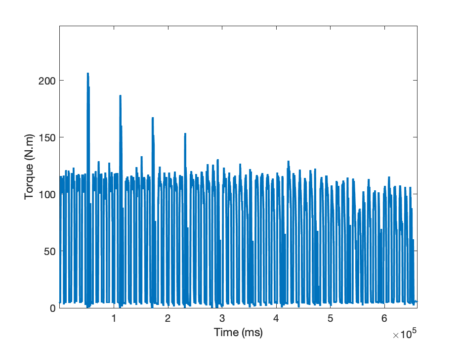
(a) All contractions

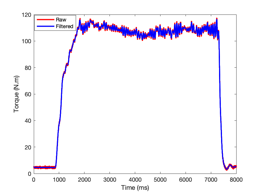
(b) One contraction

Figure 1: Muscle Contraction Data

Figure 1(a) shows that there are lots of noise data in the observations. We need to extract the useful observations. We first cut the small periods into five pieces, each piece contains about 10000 (depends on the situation) observations. For each piece, see Figure 1(b), we extract 5000 consecutive observations which the moving variance is minimum. For details, let $a_{i},i=1,\ldots,10000$ represent the 10000 observations, $A_{i}=(a_{i},\ldots,a_{i+4999})$ denotes the consecutive 5000 observations, then the minimum moving variance of $A_{s}$ can be found at $s=\mathop{\arg\min}_{\begin{subarray}{c}i\end{subarray}}(\text{Var}(A_{i}),i=1,\ldots,5001)$. Furthermore, we also use Butterworth method (Butterworth, 1930) to filter the time series before extraction. Figure 2(a) shows 52 extractions after using Butterworth Filter. Figure 2(b) shows the result of change-point detection, the two change points are 16 and 22.

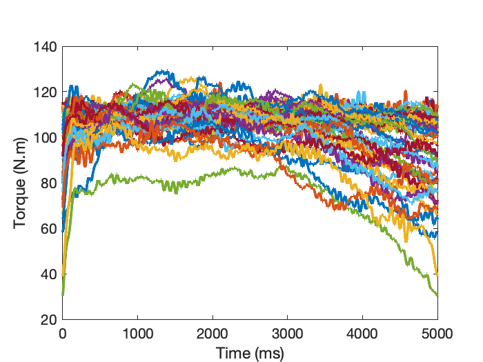
(a) All Extractions

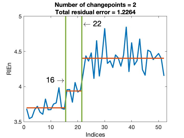
(b) $\mathfrak{E}$

Figure 2: The Results of Extractions and Change-point Detection

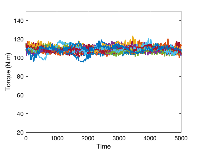
(a) Group 1

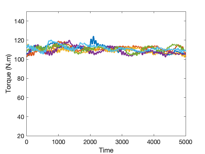
(b) Group 2

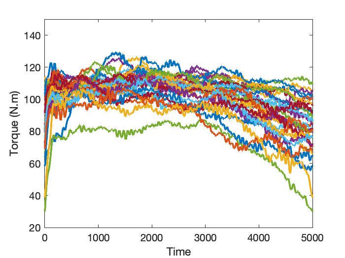
(c) Group 3

(d)

Figure 3: The Divided Groups and Change-point Detection Result for the New Simulation Dataset

To verify the performance of $\mathfrak{E}$, we further divide the time series into three groups based on Figure 2(b), namely, Group 1, 2 and 3. For each group, we obtain a seasonal ARIMA$(p,d,q)$ process. Again, 52 new time series are generated from the new seasonal ARIMA processes. Then we regard them as observations and apply our $\mathfrak{E}$ to these new observations to check whether our approach can detect the change-points correctly.

First, we need to estimate three seasonal ARIMA processes, for simplicity, let $L$ be the lag operator notation, i.e., $L^{i}x_{t}=x_{t-i}$. We found that this sport dataset is more complex than we expected, the degree of integration for three groups are 2, 2 and 2 respectively according to the Augmented Dickey-Fuller test. The real sport dataset contains seasonal effect and seasonal difference for the three groups as well, so it is a better choice to build the seasonal ARIMA processes:

$$\phi(L)\Phi(L){(1-L)}^{D}{(1-L^{s})}^{D_{s}}x_{t}=c+\theta(L)\varepsilon_{t},$$

where $\phi(L)=1-\phi_{1}L-\cdots-\phi_{p}L^{p}$ and $\theta(L)=1+\theta_{1}L+\cdots+\theta_{q}L^{q}$ represent the AR and MA operator polynomials. $\Phi(L)=1-\Phi_{p_{1}}L^{p_{1}}-\Phi_{p_{2}}L^{p_{2}}-\cdots-\Phi_{p_{s}}L^{p_{s}}$ is seasonal auto-regressive operator polynomials. ${(1-L^{s})}^{D_{s}}$ is the so-called Seasonal Difference factor, for more details of seasonal ARIMA, see Section 9.9 in Hyndman and Athanasopoulos (2013). The order of $\Phi(L)$ is determined by the spectrum analysis of time series. We use Bayesian Information Criterion (BIC) to choose the order $p$ and $q$ in $\phi(L)$ and $\theta(L)$.

Based on the average time series of each group, we have got three processes:

$$\mathbf{Process\ 1:\ } D=2,\quad D_{s}=1,\quad\hat{p}=2,$$

$$\hat{q}=2,\quad s=75,\quad c=2.9993\times 10^{-6},$$

$$\hat{\phi}(L)=1-1.9414L+0.693L^{2},$$

$$\hat{\theta}(L)=1+1.82984L+0.9931L^{2},$$

$$\hat{\Phi}(L)=1-0.02037L^{75},\ \hat{\sigma}^{2}=2\times 10^{-7}.$$

$$\mathbf{Process\ 2:\ } D=2,\quad D_{s}=1,\quad\hat{p}=2,$$

$$\hat{q}=2,\quad s=67,\quad c=2.1477\times 10^{-6},$$

$$\hat{\phi}(L)=1-1.9631L+0.9851L^{2},$$

$$\hat{\theta}(L)=1+1.9619L+0.9910L^{2},$$

$$\hat{\Phi}(L)=1+0.2818L^{67},\ \hat{\sigma}^{2}=2\times 10^{-7}.$$

$$\mathbf{Process\ 3:\ } D=2,\quad D_{s}=1,\quad\hat{p}=2,$$

$$\hat{q}=1,\quad s=81,\quad c=3.9159\times 10^{-7},$$

$$\hat{\phi}(L)=1-1.9768L+0.98801L^{2},$$

$$\hat{\Phi}(L)=1-0.1474L^{81},$$

$$\hat{\theta}(L)=1+0.3421L,\ \hat{\sigma}^{2}=2\times 10^{-7}.$$

The number of time series generated from Processes 1, 2 and 3 are 15, 6 and 31 respectively. Figure 3(d) shows our method can detect the change-points exactly at 16 and 22.

5.2 Multi-subjects Muscle Contraction Dataset

This dataset consists of 11 subjects’ muscle contraction observations. Each subject needs to perform a series of intermittent isometric contractions (six seconds for contraction and four seconds for rest) until to task failure (Pethick et al., 2016). Therefore, the number of each subject contractions is not consistent, see Table 5. The sampling frequency is 1 kHz. We found that the Figures 3(a) and 3(b) share the similar patterns, and both are significantly different to Figure 3(c). Hence, in this study, we only find one change-point. Furthermore, based on the analysis of selection of $m$ in Cases 2 and 3, the selection of $m$ is not sensitive to the change-point detection. In many research fields, ApEn is frequently employed to evaluate the complexity of signals (Richman and Moorman, 2000; Burioka et al., 2005; Pethick et al., 2016). Considering the computational complexity, we set $m=2$ to coordinate with ApEn. The change-point detections based on $\mathfrak{E}$ for each subject are summarized in Table 5. In contrast, we also obtain the change-point results based on ApEn, see Table 6. The parameter settings for ApEn follow the suggestions in Pincus (1991).

Table 5: Result of Change-point Detection Based on $\mathfrak{E}$

Subject	$N_{c}$	$CP$	$CP/N_{c}$	$\overline{\mathfrak{E}}_{1}(std.)$	$\overline{\mathfrak{E}}_{2}(std.)$	$p$-value
1	70	22	31.43%	4.0315(0.2065)	4.2406(0.2129)	4.30e-04
2	38	11	28.95%	3.6582(0.1889)	4.3606(0.2218)	1.22e-08
3	54	23	42.59%	3.8257(0.2571)	4.5578(0.2871)	4.52e-13
4	79	54	68.35%	4.1137(0.2065)	4.3692(0.2502)	5.12e-05
5	289	236	81.66%	3.4292(0.2286)	3.8779(0.2563)	1.07e-18
6	54	40	74.07%	3.8749(0.2395)	4.6409(0.1624)	5.78e-16
7	80	49	61.25%	3.6241(0.2112)	4.1233(0.2889)	2.81e-11
8	177	78	44.07%	4.1200(0.2251)	4.4312(0.1759)	4.03e-18
9	52	23	44.23%	3.7092(0.1310)	4.3786(0.2141)	1.31e-18
10	87	19	21.84%	3.9454(0.1881)	4.3561(0.1665)	1.05e-08
11	89	38	42.70%	3.9879(0.1999)	4.4219(0.2508)	3.62e-14

Table 6: Result of Change-point Detection Based on ApEn

Subject	$N_{c}$	$CP$	$CP/N_{c}$	$\overline{ApEn}_{1}(std.)$	$\overline{ApEn}_{2}(std.)$	$p$-value
1	70	68	97.14%	0.0062(0.0023)	0.0114(0.0050)	0.215
2	38	10	26.32%	0.0134(0.0043)	0.0037(0.0018)	1.15e-04
3	54	18	33.33%	0.0181(0.0067)	0.0040(0.0025)	1.33e-07
4	79	–	–	–	–	–
5	289	239	82.70%	0.0139(0.0053)	0.0073(0.0031)	1.64e-22
6	54	26	48.15%	0.0144(0.0046)	0.0040(0.0031)	5.22e-12
7	80	48	60.00%	0.0129(0.0042)	0.0059(0.0030)	4.54e-13
8	177	78	44.07%	0.0068(0.0019)	0.0047(0.0013)	8.36e-13
9	52	19	36.54%	0.0231(0.0059)	0.0046(0.0031)	1.94e-11
10	87	33	37.93%	0.0098(0.0023)	0.0063(0.0026)	5.80e-09
11	89	39	43.82%	0.0123(0.0031)	0.0047(0.0021)	4.41e-19

In Tables 5 and 6, $N_{c}$ represents the number of contractions in the series of experiments. $CP$ stands for the change-point detected by ApEn or $\mathfrak{E}$. $CP/N_{c}$ is the relative location of change-point (in percentage) compared with $N_{c}$. $\overline{\mathfrak{E}}_{1}(std.)$, $\overline{\mathfrak{E}}_{2}(std.)$, $\overline{ApEn}_{1}(std.)$ and $\overline{ApEn}_{2}(std.)$ stand for the two groups entropy averages (standard deviation) for $\mathfrak{E}$ and ApEn respectively. The last column shows the $p$-values of $t$-test for mean comparison of two groups.

In Table 5, we can conclude that the intermittent isometric contractions of each subject can be divided into two groups which are supported by the $p$-values in the last column. The averages of $\mathfrak{E}$ in the first group $\overline{\mathfrak{E}}_{1}$ are consistently smaller than $\overline{\mathfrak{E}}_{2}$. It is not surprising because muscle fatigue will increase the entropy of contraction signals (Pethick et al., 2016). According to $CP/N_{c}$, Subject 5 has the largest relative location of change-point while Subject 2’s is just 21.84%. Compared to other subjects, it means that the contraction torques are stable and Subject 5 can keep the stable contraction for a long time.

In Table 6, the “–” represents the failure of change-point detection based on ApEn. Besides, the $p$-value of $t$-test for Subject 1 is even larger than 0.1, which means the change-point, 68, is not statistically reliable. It is also worth pointing out that for Subject 10, the change-point based on ApEn is 33 but is 19 based on $\mathfrak{E}$. Figure 4 shows the two divided groups using ApEn and $\mathfrak{E}$ respectively. It is clear that the group in Figure 4(a) is more stable than the group illustrated by Figure 4(c). Moreover, there is no need to compare the averages of ApEn and $\mathfrak{E}$ because ApEn has two free parameters and is not transformation invariant. The change-points of other subjects are almost the same for both ApEn and $\mathfrak{E}$.

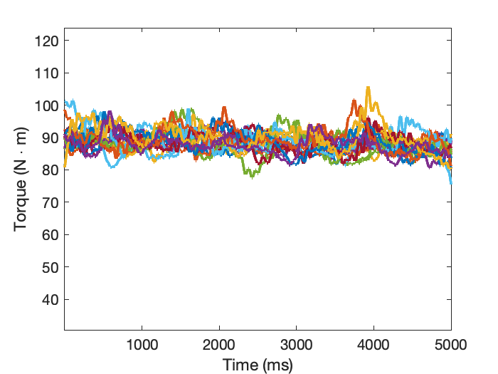
(a) $\mathfrak{E}$, First 18 Contractions

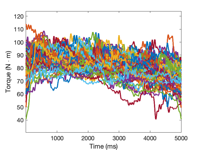
(b) $\mathfrak{E}$, Last 69 Contractions

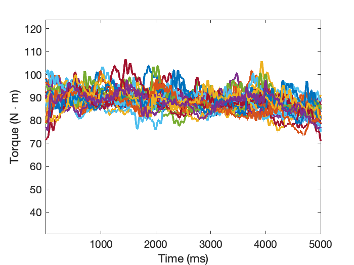
(c) ApEn, First 32 Contractions

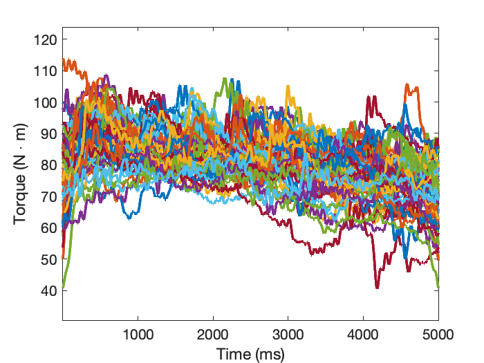
(d) ApEn, Last 55 Contractions

Figure 4: Divided Groups for Subject 10

Cases 1-3 show that the $\mathfrak{E}$ is less sensitive to the lag order $m$ and better than ApEn. Combining the results of muscle contraction data, i.e., Figure 4, Tables 5 and 6, our $\mathfrak{E}$ performs better than the ApEn.

6 Discussion

In this article, we have proposed a nonparametric relative entropy as a testing statistic to detect the change-points among intermittent time series. In nonparametric setting with weak dependence, we have developed a type of leave-one-out relative entropy. Given Assumptions 2.1 and 3.1, we have proved that the relative entropy has a limiting normal distribution with of order $\sqrt{n}h^{(m+1)/2}$. Similarly, we have also discussed the selection of lag order $m$. We suggest using BIC to select $m$. If $m$ has an upper bound, a theory of the selection of $m$ can ensure the consistency based on BIC from the point view of nonparametric regression. Three simulations have shown that the relative entropy is appropriate to summaries the information of a time series. Based on RlEn, one can find the change-points among intermittent time series with high accurateness. One real data analysis has shown that our approach is effective in terms of change-point detection in practice as well.

Data and Code Availability

The code is available at GitHub repository: https://github.com/Jieli12/RlEn. Please contact the corresponding author for accessing to the real sports data.

Competing interests

We declare that we have no competing interests.

Appendix A Relative Entropy for Stationary AR(2) Process

Without loss of generality, let

$$x_{i}=\phi_{1}x_{i-1}+\phi_{2}x_{i-2}+\varepsilon_{i},$$ (21)

represent the AR$(2)$ process without intercept, where $\varepsilon_{i}$ is Gaussian white noise with zero mean and variance $\sigma^{2}$. Suppose $-1<\phi_{2}<1-\left|\phi_{1}\right|$, then process (21) is stationary. Let $\gamma_{0}=E(X_{i}^{2})$, $\gamma_{1}=E(X_{i}X_{i-1})$ and $\gamma_{2}=E(X_{i}X_{i-2})$. By (21), we have the following Yule-Walker equations: $\gamma_{0}=\gamma_{0}\,{\phi_{1}}^{2}+2\,\gamma_{1}\,\phi_{1}\,\phi_{2}+\gamma_{0}\,{\phi_{2}}^{2}+\sigma^{2}$, $\gamma_{1}=\gamma_{0}\,\phi_{1}+\gamma_{1}\,\phi_{2}$ and $\gamma_{2}=\gamma_{1}\,\phi_{1}+\gamma_{0}\,\phi_{2}$. Solving the above linear equations, we can get $\gamma_{0}=\sigma^{2}\,(\phi_{2}-1)/\phi_{c}$, $\gamma_{1}=-\phi_{1}\,\sigma^{2}/\phi_{c}$ and $\gamma_{2}=-\sigma^{2}\,({\phi_{1}}^{2}-{\phi_{2}}^{2}+\phi_{2})/\phi_{c}$ where $\phi_{c}=\left(\phi_{2}+1\right)\,\left({\phi_{1}}^{2}-{\phi_{2}}^{2}+2\,\phi_{2}-1\right)$. As $\varepsilon_{i}$ is the Gaussian white noise, $X_{i},X_{i-1},X_{i-2}$ have the following density function, namely,

$$f(x_{i},x_{i-1},x_{i-2})={(2\pi)}^{-\frac{3}{2}}{\left|\Sigma\right|}^{-\frac{1}{2}}\exp\left(-(x_{i},x_{i-1},x_{i-2})\Sigma^{-1}{(x_{i},x_{i-1},x_{i-2})}^{T}/2\right),$$

where

$$\Sigma=\begin{bmatrix}\gamma_{0}&\gamma_{1}&\gamma_{2}\\ \gamma_{1}&\gamma_{0}&\gamma_{1}\\ \gamma_{2}&\gamma_{1}&\gamma_{0}\end{bmatrix},\qquad\Sigma^{-1}=\frac{1}{\sigma^{2}}\left(\begin{array}[]{ccc}1&-\phi_{1}&-\phi_{2}\\ -\phi_{1}&{\phi_{1}}^{2}-{\phi_{2}}^{2}+1&-\phi_{1}\\ -\phi_{2}&-\phi_{1}&1\end{array}\right),$$

and $\left|\Sigma\right|=-\sigma^{6}/(\phi_{c}\left(\phi_{2}+1\right))$. Therefore, the entropy of $f(x_{i},x_{i-1},x_{i-2})$ is

$$\text{En}(f) =-\iiint f(x_{i},x_{i-1},x_{i-2})\log\left(f(x_{i},x_{i-1},x_{i-2})\right)\,\mathrm{d}x_{i}\,\mathrm{d}x_{i-1}\,\mathrm{d}x_{i-2},$$ (22)

$$=2^{-1}\log\left({(2\pi e)}^{3}\left|\Sigma\right|\right).$$

By (21) and given $x_{i-1},x_{i-2}$, we can obtain the conditional density:

$$g(x_{i}|x_{i-1},x_{i-2})={(2\pi)}^{-1/2}{\left|\sigma\right|}^{-1}\exp\left(-{(x_{i}-\phi_{1}x_{i-1}-\phi_{2}x_{i-2})}^{2}/(2\sigma^{2})\right).$$

The conditional entropy is

$$\text{CoEn}(f,g) =-\iiint f(x_{i},x_{i-1},x_{i-2})\log\left(g(x_{i}|x_{i-1},x_{i-2})\right)\,\mathrm{d}x_{i}\,\mathrm{d}x_{i-1}\,\mathrm{d}x_{i-2},$$

$$=\frac{1}{2}\log(2\pi)+\log(\sigma)+\frac{1}{2\sigma^{2}}E\left[{(x_{i}-\phi_{1}x_{i-1}-\phi_{2}x_{i-2})}^{2}\right],$$

$$=\frac{1}{2}\log(2\pi)+\log(\sigma)+\frac{1}{2\sigma^{2}}E\left[y^{2}\right],$$

where $y=c^{T}\mathbf{x}$, $c^{T}=(1,-\phi_{1},-\phi_{2})$, $\mathbf{x}={(x_{i},x_{i-1},x_{i-2})}^{T}$. Apparently, $y\sim N(0,c^{T}\Sigma c)$. It is easy to verify that $c^{T}\Sigma c=\sigma^{2}$, so

$$\text{CoEn}(f,g)=2^{-1}\log(2\pi e)+\log(\sigma).$$ (23)

We also notice that the density of $x_{i}$ is $g(x_{i})={(2\pi)}^{-1/2}{\left|\gamma_{0}\right|}^{-1/2}\exp\left(-x_{i}^{2}/2\gamma_{0}\right)$. Finally, one can obtain the relative entropy

$$\text{RlEn}(f,g) =2^{-1}\log\left((\phi_{2}-1)/\phi_{c}\right).$$ (24)

Comparing Entropy (22), Conditional Entropy (23) with Relative Entropy (24), we conclude that RlEn is determined by the coefficients of autoregression coefficients and does not include the variance of noise in the AR(2) process.

Appendix B Background-noise-free

For simplicity, we only show the property of background-noise-free for AR$(p)$ process. It is easy to extend to the general case such as MA$(q)$, ARMA$(p,q)$ process. Without loss of generality, let the AR$(p)$ process with zero mean be

$$x_{i}=\phi_{1}x_{i-1}+\phi_{2}x_{i-2}+\cdots+\phi_{p}x_{i-p}+\varepsilon_{i},$$ (25)

where $\phi_{1},\ldots,\phi_{p}$ are autoregression coefficients, $\varepsilon_{i}$ is the Gaussian white noise with zero mean and variance $\sigma^{2}$, $\{x_{i}\}_{1\leq i\leq n}$ and $\{\varepsilon_{i}\}_{1\leq i\leq n}$ are dependent. Let $\mathbf{x}_{m+1}={(x_{i},\ldots,x_{i+m})}^{\top}$, $\mathbf{x}_{m+1-s}={(x_{i},\ldots,x_{i+m-s})}^{\top}$ and $\mathbf{x}_{s}={(x_{i+m-s+1},\ldots,x_{i+m})}^{\top}$. $\gamma_{k}=E(x_{i}x_{i-k}),k=0,\pm 1,\pm 2,\ldots$ represent the auto-covariance functions, apparently $\gamma_{k}=\gamma_{-k}$. Next, define $\rho_{k}=\gamma_{k}/\gamma_{0},k=0,\pm 1,\pm 2,\ldots$ as the auto-correlation functions. Hence, we have the following proposition.

Proposition B.1.

Supposed $\{x_{i}\}$ is a time series from the stationary AR$(p)$ process defined in (25), $\varepsilon_{i}$ is the Gaussian white noise with zero mean and variance $\sigma^{2}$, then we have

$$\mathcal{I}_{s}\left(\mathbf{x}_{m+1}\right)=\frac{1}{2}\log\left(\frac{\left|R_{11;ms}\right|\left|R_{22;ms}\right|}{\left|R_{m}\right|}\right),\quad 1\leq s\leq m,$$ (26)

which is independent of $\sigma^{2}$, where $\left|\cdot\right|$ is a matrix determinant operator.

To prove this proposition, we need the following lemma

Lemma B.1.

If multivariate variable $\mathbf{x}\sim N_{p}(\mu,\Sigma)$, then the entropy of $\mathbf{x}$, denoted as $h(\mathbf{x})$, is

$$h(\mathbf{x})=\frac{1}{2}\log\left({(2\pi e)}^{p}\left|\Sigma\right|\right).$$

Proof.

By the definition of continuous entropy, we have

$$h(\mathbf{x}) =-\int_{\mathbb{R}^{p}}f(\mathbf{x})\log\left(f(\mathbf{x})\right)d\mathbf{x},$$

$$=\frac{p}{2}\log(2\pi)+\frac{1}{2}\log(\left|\Sigma\right|)+\frac{1}{2}\mathbf{E}\left[{\left(\mathbf{x}-\mu\right)}^{T}\Sigma^{-1}\left(\mathbf{x}-\mu\right)\right],$$

$$=\frac{1}{2}\log\left({(2\pi e)}^{p}\left|\Sigma\right|\right),$$

this completes the proof. ∎

Let $\Sigma_{m},\Sigma_{11;ms},\Sigma_{22;ms}$ represent the auto-covariance matrices of vectors $\mathbf{x}_{m+1}$, $\mathbf{x}_{m+1-s}$ and $\mathbf{x}_{s}$ respectively, $\Sigma_{12;ms}$ is the covariance matrix between $\mathbf{x}_{m+1-s}$ and $\mathbf{x}_{s}$, i.e.,

$$\Sigma_{m}=\begin{bmatrix}\gamma_{0}&\gamma_{1}&\gamma_{2}&\cdots&\gamma_{m}\\ \gamma_{1}&\gamma_{0}&\gamma_{1}&\cdots&\gamma_{m-1}\\ \gamma_{2}&\gamma_{1}&\gamma_{0}&\cdots&\gamma_{m-2}\\ \vdots&\vdots&\vdots&\vdots&\vdots\\ \gamma_{m}&\gamma_{m-1}&\gamma_{m-2}&\cdots&\gamma_{0}\end{bmatrix},\Sigma_{11;ms}=\begin{bmatrix}\gamma_{0}&\gamma_{1}&\cdots&\gamma_{m-s}\\ \gamma_{1}&\gamma_{0}&\cdots&\gamma_{m-s-1}\\ \gamma_{2}&\gamma_{1}&\cdots&\gamma_{m-s-2}\\ \vdots&\vdots&\vdots&\vdots\\ \gamma_{m-s}&\gamma_{m-s-1}&\cdots&\gamma_{0}\end{bmatrix},$$

and

$$\Sigma_{22;ms}=\begin{bmatrix}\gamma_{0}&\gamma_{1}&\cdots&\gamma_{s-1}\\ \gamma_{1}&\gamma_{0}&\cdots&\gamma_{s-2}\\ \gamma_{2}&\gamma_{1}&\cdots&\gamma_{s-3}\\ \vdots&\vdots&\vdots&\vdots\\ \gamma_{s-1}&\gamma_{s-2}&\cdots&\gamma_{0}\end{bmatrix},\Sigma_{12;ms}=\begin{bmatrix}\gamma_{m-s+1}&\gamma_{m-s+2}&\cdots&\gamma_{m}\\ \gamma_{m-s}&\gamma_{m-s+1}&\cdots&\gamma_{m-1}\\ \gamma_{m-s-1}&\gamma_{m-s}&\cdots&\gamma_{m-2}\\ \vdots&\vdots&\vdots&\vdots\\ \gamma_{1}&\gamma_{2}&\cdots&\gamma_{s}\end{bmatrix}.$$

For simplicity, we have

$$\Sigma_{m}=\begin{bmatrix}\Sigma_{11;ms}&\Sigma_{12;ms}\\ \Sigma_{21;ms}&\Sigma_{22;ms}\end{bmatrix},$$

we also notice that $R_{m}=\gamma^{-1}_{0}\Sigma_{m}$, $R_{11;ms}=\gamma^{-1}_{0}\Sigma_{11;ms}$, $R_{12;ms}=\gamma^{-1}_{0}\Sigma_{12;ms}$, $R_{22;s}=\gamma^{-1}_{0}\Sigma_{22;ms}$. Based on these facts, we now prove Proposition B.1.

Proof of Proposition B.1.

Since $\varepsilon_{i}$ is the Gaussian white noise, the distribution of $\mathbf{x}_{m+1}$, $\mathbf{x}_{m+1-s}$ and $\mathbf{x}_{s}$ are multivariate Gaussian with covariance matrices $\Sigma_{m},\Sigma_{11;ms},\Sigma_{22;ms}$ respectively. By Lemma B.1, we can obtain the following results: $h\left(\mathbf{x}_{m+1}\right)=2^{-1}\log\left({(2\pi e)}^{m+1}\left|\Sigma_{m}\right|\right)$, $h\left(\mathbf{x}_{s}\right)=2^{-1}\log\left({(2\pi e)}^{s}\left|\Sigma_{22;ms}\right|\right)$ and $h\left(\mathbf{x}_{m+1-s}\right)=2^{-1}\log\left({(2\pi e)}^{m+1-s}\left|\Sigma_{11;ms}\right|\right)$. The relative entropy can be expressed as

$$\mathcal{I}_{s}\left(\mathbf{x}_{m+1}\right) =\text{RlEn}_{s}=\int_{\mathbb{R}^{m+1}}f\left(\mathbf{x}_{m+1}\right)\log\left(\frac{f\left(\mathbf{x}_{m+1}\right)}{g\left(\mathbf{x}_{m+1-s}\right)g\left(\mathbf{x}_{s}\right)}\right)d\mathbf{x}_{m+1},$$

$$=\frac{1}{2}\log\left(\frac{\left|R_{11;ms}\right|\left|R_{22;ms}\right|}{\left|R_{m}\right|}\right),\quad 1\leq s\leq m,\quad m\geq 1.$$

By the Yule-Walker equations,

$$\begin{bmatrix}\rho_{1}\\ \rho_{2}\\ \rho_{3}\\ \vdots\\ \rho_{p}\end{bmatrix}=\begin{bmatrix}1&\rho_{1}&\rho_{2}&\cdots&\rho_{p-1}\\ \rho_{1}&{1}&\rho_{2}&\cdots&\rho_{p-2}\\ \rho_{2}&\rho_{1}&1&\cdots&\rho_{p-3}\\ \vdots&\vdots&\vdots&\vdots&\vdots\\ \rho_{p-1}&\rho_{p-2}&\rho_{p-3}&\cdots&1\\ \end{bmatrix}\begin{bmatrix}\phi_{1}\\ \phi_{2}\\ \phi_{3}\\ \vdots\\ \phi_{p}\end{bmatrix},$$

the autocorrelation $\rho_{i},i=1,2,\ldots,\infty$ are totally determined by coefficient $\phi_{k},k=1,\ldots,p$. Hence, $\mathcal{I}_{s}(\mathbf{x}_{m+1})$ is a function of $\phi_{k},k=1,\ldots,p$. As $\{x_{i}\}$ and $\{\varepsilon_{i}\}$ are independent, the autocorrelation function of $\{x_{i}\}$ is independent of $\sigma$ which implies $\mathcal{I}_{s}(\mathbf{x}_{m+1})$ is independent of $\sigma$ as well which completes the proof. ∎

Appendix C Lag order selection and proof

Proof of Theorem 2.2.

The proof is based on the proofs of Vieu (1995) and Shao (1997). First, we construct a new equation $\sigma^{2}_{\lambda}(m)=\hat{\sigma}^{2}(m)[1+\lambda(m,\hat{h}_{m})]$, where $\lambda(m,\hat{h}_{m})=v(m,\hat{h}_{m})\log(n)/n$. We can regard $\lambda(m,\hat{h}_{m})$ as a penalty part in $\sigma^{2}_{\lambda}(m)$, when $\lambda(m,\hat{h}_{m})\rightarrow 0$, minimizing $BIC(m)$ is equivalent to minimizing $\sigma^{2}_{\lambda}(m)$ based on the fact that $\log(1+x)\approx x$ as $x\rightarrow 0$. This proof skill is frequently adopted in discussion of BIC or AIC consistency, see, for example, Shibata (1981, p.46), Vieu (1995, 314) and Shao (1997, 232). Therefore, the sketch of our proof can be summarized into the following two steps: (1) We need to discuss the consistency of lag order selected via $\hat{\sigma}^{2}(m)$; (2) We extend the result to the penalty version $\sigma^{2}_{\lambda}(m)$ with controlling $\lambda(m,\hat{h}_{m})\rightarrow 0$ in an appropriate rate. This proof is very similar to that in lag order selection (Vieu, 1995) except the definitions of $\hat{\sigma}^{2}(m)$ and $\lambda(m,\hat{h}_{m})$. Next, we introduce the conditions used in our proof.

1. The time series ${\{X_{i}\}}_{i\in\mathbb{N}}$ is $\alpha$-mixing, the mixing coefficient $\alpha(n)$ satisfies: $\exists\ s>0,\exists\ 0<t<1,\forall\ n\geq 1,\alpha(n)\leq st^{n}$.

2. For each $1\leq m<M$, there exists the nonlinear autoregression functions such that

   $$x_{i+m}=\mathfrak{F}\left(\mathbf{X}_{i;m}\right)+\varepsilon_{i,m},$$

   where $\mathbf{X}_{i;m}$ is independent of $\varepsilon_{i,m}$ and $\varepsilon_{i,m},i=1,\ldots,n$ are noise with mean zero.

3. The unknown function $\mathfrak{F}$ has second-order continuous derivation.

4. $\forall\ q\geq 1,\exists\ \mathbb{M}_{q}$ such that for any $i,\mathbb{E}{\left|X_{i}\right|}^{q}\leq\mathbb{M}_{q}<\infty$.

5. Given $m$, for some $0<\gamma_{m}<\infty$ and some $0<\eta_{m}<1/(4+m)$, the bandwidth satisfies:

   $$h_{*}\in\mathcal{H}_{n,m}=\left[\gamma^{-1}_{m}n^{-\eta_{m}-1/(4+m)},\gamma_{m}n^{\eta_{m}-1/(4+m)}\right].$$

6. $\lambda(m,\hat{h}_{m})$ is of order $\log(n)/(n{(h_{*})}^{m})$.

7. $m$ could be arbitrary large but has an upper bound $M$.

Conditions (C1)–(C6) are quoted from Vieu (1995, 310–311) with appropriate adjustments for our circumstance. Condition (C7) controls the upper bound $M$ to coordinate the proof of $\mathfrak{E}$ in Appendix D. Given lag order $m,1\leq m\leq M$ and the underlying lag order $m_{0}$, we define the distance between $\mathfrak{F}(\mathbf{X}_{i;m_{0}})$ and $\hat{\mathfrak{F}}(\mathbf{X}_{i;m},h_{*})$ by

$$\sigma_{0}^{2}(m,h_{*})=\frac{1}{N-\max(m,m_{0})}\sum_{i=1}^{\max(m,m_{0})}{\left[\mathfrak{F}\left(\mathbf{X}_{i;m_{0}}\right)-\hat{\mathfrak{F}}\left(\mathbf{X}_{i;m},h_{*}\right)\right]}^{2}.$$

Furthermore, let $\sigma_{0}^{2}(m)=\inf_{h_{*}\in\mathcal{H}}\sigma_{0}^{2}(m,h_{*})$, we have

Lemma C.1.

Given Conditions (C1)–(C5), Assumption 2.1 and Assumption 3.1, the nonlinear autoregression process (3) has underlying lag order $m_{0}$ and $m_{0}\in\left\{1,\ldots,M\right\}$, then we have

1. $\sigma_{0}^{2}(m_{0})\rightarrow 0$, a.e.,

2. For $1\leq m<m_{0}$, there exists real positive constant $c_{m}>0$ such that

   $$\hat{\sigma}^{2}(m)-\hat{\sigma}^{2}(m_{0})\geq c_{m},\quad a.s.,$$

3. For $m_{0}<m\leq M$, $\exists\ c_{0}>0\ s.t.$ $\hat{\sigma}^{2}(m_{0})-c_{0}\geq 0$, a.s. and

   $$\frac{\hat{\sigma}^{2}(m)-c_{0}}{\hat{\sigma}^{2}(m_{0})-c_{0}}\rightarrow+\infty,\quad a.s.$$

Proof of Lemma C.1.

This proof employs the same techniques used in Lemma 1, Lemma 2 and Theorem 3 in Vieu (1995). It can be regarded as a special case of Vieu (1995) except the upper bound $M$. Give $m$, $n=N-m$, the average square predict error of nonlinear autoregression is defined as

$$\sigma^{2}(m,h_{*})=\frac{1}{n}\sum_{i=1}^{n}{\left[\mathfrak{F}\left(\mathbf{X}_{i;m}\right)-\hat{\mathfrak{F}}\left(\mathbf{X}_{i;m},h_{*}\right)\right]}^{2}.$$

Under Assumptions 2.1 and 3.1, we can rewrite the average square predict error (e.g., Li and Racine, 2007, 83–85) as

$$\sigma^{2}(m,h_{\ast})=\alpha_{1m}\frac{1}{nh_{*}^{m}}+\alpha_{2m}mh_{*}^{4}+o\left(\frac{1}{nh_{*}^{m}}+h_{*}^{4}\right),\quad a.s.,$$ (27)

where $\alpha_{1m}$ and $\alpha_{2m}$ are constant. We can easily obtain the optimal bandwidth if we minimize the first two leading terms in equation (27), denoted as

$$\hat{h}_{m}={\left(\frac{4\alpha_{2m}}{\alpha_{1m}}n\right)}^{-\frac{1}{4+m}}.$$

Finally, we get

$$\sigma^{2}(m)=\inf_{h_{*}\in\mathcal{H}_{n,m}}\sigma^{2}(m,h_{*})=\alpha_{3m}n^{-\frac{4}{4+m}}+o\left(n^{-\frac{4}{4+m}}\right),\quad a.s.,$$ (28)

where $\alpha_{3m}$ is a constant. Especially, when $m=m_{0}$, then $\sigma^{2}(m)=\sigma^{2}_{0}(m_{0})$, immediately, $\sigma_{0}^{2}(m_{0})\rightarrow 0$ holds almost surely. This completes the proof of (a).

Proof of (b). For given $m$, $1\leq m<m_{0}$, let $\hat{h}_{m,cv}=\operatorname*{arg\,min}_{h_{*}\in\mathcal{H}_{n,m}}\hat{\sigma}^{2}(m,h_{*})$, the bandwidth selected by least square cross-validation is still of order $n^{-1/(4+m)}$ as $\hat{h}_{m}$ (Vieu, 1991; Hall et al., 2004), so $\hat{h}_{m,cv}\in\mathcal{H}_{n,m}$, we have

$$\frac{\sigma^{2}(m,\hat{h}_{m,cv})}{\inf\limits_{h_{*}\in\mathcal{H}_{n,m}}\sigma^{2}(m,h_{*})}\rightarrow 1,\quad a.s.$$ (29)

In the proof of this property, Vieu (1991) and Vieu (1995) employed the following statement for nonlinear autoregression:

$$\hat{\sigma}^{2}(m,h_{*})-\sigma^{2}(m,h_{*})=\frac{1}{n}\sum_{i=1}^{n}\varepsilon^{2}_{i,m}+o\left(\sigma^{2}(m,h_{*})\right),\quad a.s.,$$ (30)

where the operation $o(\cdot)$ is uniform over $h_{*}\in\mathcal{H}_{n,m}$. Therefore, by equation (28) and equation (29), $\forall$ $m$, $1\leq m<m_{0}$, we have $\sigma^{2}(m,\hat{h}_{m,cv})=o(n^{-4/(4+m)})$ almost surely. Then, minimizing equation (30), we obtain for any $1\leq m<m_{0}$

$$\hat{\sigma}^{2}(m)=\frac{1}{n}\sum_{i=1}^{n}\varepsilon^{2}_{i,m}+o(1),\quad a.s.$$ (31)

Let $\delta_{m}=\text{Var}(\varepsilon_{i,m})$ and $c_{m}=\delta_{m}-\delta_{m_{0}}$, by equation (31), we have $\hat{\sigma}^{2}(m)-\hat{\sigma}^{2}(m_{0})\rightarrow c_{m}$, a.s., and $c_{m}>0$ because from (C5) and Assumption 3.1, we know $c_{m}\geq\text{ Var }[\mathbb{E}(x_{i+m}|\mathbf{X}_{i;m_{0}})-\mathbb{E}(x_{i+m}|\mathbf{X}_{i;m})]$, because $1\leq m<m_{0}$, so $\text{ Var }[\mathbb{E}(x_{i+m}|\mathbf{X}_{i;m_{0}})-\mathbb{E}(x_{i+m}|\mathbf{X}_{i;m})]>0$ which completes the proof (b).

Proof of (c). For $m_{0}<m\leq M$, replacing $h_{*}$ in equation (30) with $\hat{h}_{m,cv}$, we obtain

$$\hat{\sigma}^{2}(m)-\sigma^{2}(m,\hat{h}_{m,cv})=\frac{1}{n}\sum_{i=1}^{n}\varepsilon^{2}_{i,m}+o\left(n^{-4/(4+m)}\right),\quad a.s.$$

We also note that (29) implies

$$\sigma^{2}(m,\hat{h}_{m,cv})=\inf\limits_{h_{*}\in\mathcal{H}_{n,m}}\sigma^{2}(m,h_{*})+o\left(n^{-4/(4+m)}\right),\quad a.s.,$$

therefore

$$\hat{\sigma}^{2}(m)=\sigma^{2}_{0}(m)+\frac{1}{n}\sum_{i=1}^{n}\varepsilon^{2}_{i,m}+o\left(n^{-4/(4+m)}\right),\quad a.s.$$ (32)

Like the discussion in Vieu (1995), by Bernstein’s inequality for $\alpha$-mixing, for example, see the Theorem 3.1 in Roussas and Ioannides (1988), we have

$$\frac{1}{N-m_{0}}\sum_{i=1}^{N-m_{0}}\varepsilon^{2}_{i,m_{0}}-\text{Var}(\varepsilon_{i,m_{0}})=o\left(n^{-4/(4+m_{0})}\right),\quad a.s.$$ (33)

Combining (32) and (33), we get

$$\frac{\left|\hat{\sigma}^{2}(m)-c_{0}\right|}{\left|\hat{\sigma}^{2}(m_{0})-c_{0}\right|}=\frac{\sigma^{2}_{0}(m)}{\sigma^{2}_{0}(m_{0})}+o\left(\frac{\sigma^{2}_{0}(m)}{\sigma^{2}_{0}(m_{0})}\right),\quad a.s.,$$

where $c_{0}=\text{Var}(\varepsilon_{i,m_{0}})$. By the fact (28), we have $\sigma^{2}_{0}(m)/\sigma^{2}_{0}(m_{0})\rightarrow\infty$ almost surely. Immediately, by (32), we can conclude $\hat{\sigma}^{2}(m_{0})-c_{0}\geq 0$, a.s., because $\sigma^{2}_{0}(m)$ is positive. This completes the proof. ∎

Let $\bar{m}=\operatorname*{arg\,min}\hat{\sigma}^{2}(m)$, based on Lemma C.1, we immediately have

$$\sigma^{2}_{0}(\bar{m})/\sigma^{2}_{0}(m_{0})\rightarrow 1,\quad a.s.$$

Moreover, we add the penalty part to $\hat{\sigma}^{2}(m)$, i.e., $\sigma^{2}_{\lambda}(m)=\hat{\sigma}^{2}(m)[1+\lambda(m,\hat{h}_{m})]$, where $\lambda(m,\hat{h}_{m})=v(m,\hat{h}_{m})\log(n)/n$. Based on Lemma 2.1, Condition (C6) makes sure that the penalty part is not arbitrary large compared with 0. Based on Lemma C.1, previous discussion and Condition (C7), we have

$$\max_{m=1,\ldots,M}\frac{\left|\sigma^{2}_{\lambda}(m)-\hat{\sigma}^{2}(m)\right|}{\sigma^{2}_{0}(m)} =\frac{\log(n)}{n^{\frac{4}{4+m}}}\leq\frac{\log(n)}{n^{\frac{4}{4+O\left(\sqrt{\log(n)}\right)}}}=o(1),\quad a.s.$$ (34)

Let $\hat{m}=\operatorname*{arg\,min}\sigma_{\lambda}^{2}(m)$, we have $\sigma^{2}_{0}(\hat{m}_{\lambda})/\sigma^{2}_{0}(m_{0})\rightarrow 1$ almost surely. Because the previous results are almost surely convergence, so

$$P(\hat{m}=m_{0})\rightarrow 1,$$

holds as well which completes the whole proof. ∎

Note: Vieu (1995) claimed $M=O(\log(n))$, however, our result shows that $M$ is at least of order $O(\sqrt{\log(n)})$, see equation (34). Furthermore, if one want to control $M$ to tend to infinity not as fast as $O(\sqrt{\log(n)})$, the order of $M$ could be $O(\log(\log(n)))$. However, in order to keep $M$ consistent in the proof of relative entropy theory, we sacrifice the relaxation of $m$ to infinity discussed above.

Appendix D Consistency of nonparametric complexity measure

Lemma D.1.

Given $\mathbb{H}_{0}$, under Assumptions 2.1 and 3.1, if $nh^{m}/\log{n}\rightarrow\infty$, $h\rightarrow 0$ and $m<M$. The order of the remainder term in equation (9) is

$$O_{p}\left(n^{-3/2}h^{-3m/2}{(\log{n})}^{1/2}+m^{2}h^{6}\right).$$

Proof of Lemma D.1..

Under Assumptions 2.1 and 3.1, we can obtain the uniform rates of convergence for multivariate kernel density estimator (e.g., Li and Racine, 2007, p.30–32). For $\mathbf{z}\in\mathbbm{I}^{m}$, it follows that

$$\sup_{\mathbf{z}\in\mathbbm{I}^{m}}\left|\hat{g}(\mathbf{z})-g(\mathbf{z})\right|=O_{p}\left(\frac{{(\log{n})}^{1/2}}{n^{1/2}h^{m/2}}+mh^{2}\right),$$ (35)

and

$$\sup_{\mathbf{z}\in\mathbbm{I}^{m}}\mathbb{E}\left\{{\left[\hat{g}(\mathbf{z})-g(\mathbf{z})\right]}^{2}\right\}=O\left(n^{-1}h^{-m}+mh^{4}\right).$$ (36)

Using (35) and (36), we have

$$\frac{1}{n}\sum_{i=1}^{n}{\left|\hat{g}\left(\mathbf{x}_{i;m}\right)-g\left(\mathbf{x}_{i;m}\right)\right|}^{3}$$ (37)

$$\quad\leq\sup_{\mathbf{x}_{i;m}\in\mathbbm{I}^{m}}\left|\hat{g}\left(\mathbf{x}_{i;m}\right)-g\left(\mathbf{x}_{i;m}\right)\right|\left\{\frac{1}{n}\sum_{i=1}^{n}{\left[\hat{g}\left(\mathbf{x}_{i;m}\right)-g\left(\mathbf{x}_{i;m}\right)\right]}^{2}\right\},$$

$$\quad=O_{p}\left(\frac{{(\log{n})}^{1/2}}{n^{3/2}h^{3m/2}}+m^{2}h^{6}\right).$$

Then by (37) and the inequality $\left|\log(1+x)-x+\frac{1}{2}x^{2}\right|\leq{\left|x\right|}^{3}$, obviously we have

$$\left|\hat{I}_{m}(\hat{g},g)-\hat{W}_{1S}(m)+\frac{1}{2}\hat{W}_{2S}(m)\right|$$ (38)

$$\quad\leq\frac{1}{n}\sum_{i\in S(m)}{\left|\frac{\hat{g}\left(\mathbf{x}_{i;m}\right)-g\left(\mathbf{x}_{i;m}\right)}{g\left(\mathbf{x}_{i;m}\right)}\right|}^{3,}$$

$$\quad=O_{p}\left(\frac{{(\log{n})}^{1/2}}{n^{3/2}h^{3m/2}}+m^{2}h^{6}\right),$$

where

$$\hat{W}_{1S}(m)=\frac{1}{n}\sum_{i\in S(m)}\left[\frac{\hat{g}\left(\mathbf{x}_{i;m}\right)-g\left(\mathbf{x}_{i;m}\right)}{g\left(\mathbf{x}_{i;m}\right)}\right],$$

and

$$\hat{W}_{2S}(m)=\sum_{i\in S(m)}{\left[\frac{\hat{g}\left(\mathbf{x}_{i;m}\right)-g\left(\mathbf{x}_{i;m}\right)}{g\left(\mathbf{x}_{i;m}\right)}\right]}^{2}.$$

Note that the definitions of $\hat{W}_{1}(m)$ and $\hat{W}_{2}(m)$ include the summation of $n$ observations. The difference is

$$\left[\hat{W}_{1S}(m)-\frac{1}{2}\hat{W}_{2S}(m)\right]-\left[\hat{W}_{1}(m)-\frac{1}{2}\hat{W}_{2}(m)\right]$$

$$\quad=O_{p}\left[\frac{1}{n}\sum_{i=1}^{n}P\left(i\not\in S(m)\right)\right],$$ (39)

$$\quad=O_{p}\left[\frac{1}{n}\sum_{i=1}^{n}\mathbb{E}{\left|\frac{\hat{g}\left(\mathbf{x}_{i;m}\right)-g\left(\mathbf{x}_{i;m}\right)}{g\left(\mathbf{x}_{i;m}\right)}\right|}^{3}\right],$$ (40)

$$\quad=O_{p}\left(\frac{{(\log{n})}^{1/2}}{n^{3/2}h^{3m/2}}+m^{2}h^{6}\right).$$ (41)

Step (39) to step (40) is based on the fact that

$$P\left(i\not\in S(m)\right) =P\left(\hat{g}\left(\mathbf{x}_{i;m}\right)\leq 0\right),$$

$$\leq P\left[\left|\hat{g}\left(\mathbf{x}_{i;m}\right)-g\left(\mathbf{x}_{i;m}\right)\right|>g\left(\mathbf{x}_{i;m}\right)\right],$$

$$\leq\mathbb{E}{\left|\frac{\hat{g}\left(\mathbf{x}_{i;m}\right)-g\left(\mathbf{x}_{i;m}\right)}{g\left(\mathbf{x}_{i;m}\right)}\right|}^{3}.$$

Combining equations (38) and (41), we complete the proof of this lemma. ∎

Lemma D.2.

Given Assumptions 2.1 and 3.1, if $h\rightarrow 0$ and $m<M$. Then under $\mathbb{H}_{0}$, we have $P(\lim_{n\rightarrow\infty}\hat{\Gamma}(m)=0)=1$.

Proof of Lemma D.2.

Firstly, we give a similar result for univariate kernel, then we extend this result to multivariate kernel. For any $x,y\in[0,1]$, denote $\gamma_{1}(x,y)=\int_{0}^{1}[K_{h}^{J}(x^{*},y)-\int_{0}^{1}K_{h}^{J}(x^{*},y^{*})g_{1}(y^{*})dy^{*}]dx^{*}/g_{1}(x)$. The numerator of $\gamma_{1}(x,y)$ includes two terms. The first term can be expanded as

$$\int_{0}^{1}K_{h}^{J}\left(x^{*}-y\right)\,\mathrm{d}x^{*}$$ (42)

$$\quad=\int_{0}^{h}K_{h}^{J}\left(x^{*}-y\right)\,\mathrm{d}x^{*}+\int_{1-h}^{1}K_{h}^{J}\left(x^{*}-y\right)\,\mathrm{d}x^{*}+\int_{h}^{1-h}K_{h}\left(x^{*}-y\right)\,\mathrm{d}x^{*},$$

when $n\rightarrow\infty$, then $h\rightarrow 0$ such that $y/h\rightarrow\infty$ and $(1-y)/h\rightarrow\infty$ for any $y\in(0,1)$, see Appendix A in Hong and White (2005). Using $K(\cdot)$ having bounded support $[-1,1]$ and change of variable, when $n$ is sufficient large, the first and second terms in equation (42) are zero, and the third term is 1. When $n$ is sufficiently large, the term

$$\int_{0}^{1}\int_{0}^{1}K_{h}^{J}(x^{*},y^{*})g_{1}(y^{*})dy^{*}dx^{*}$$ (43)

$$\quad=\int_{0}^{1}g_{1}(y^{*})\int_{0}^{1}K_{h}^{J}(x^{*},y^{*})dx^{*}dy^{*}$$

$$\quad=\int_{0}^{1}g_{1}(y^{*})\cdot 1dy^{*}=1,$$

as well. Therefore, when $n$ is sufficiently large, $\gamma_{1}(x,y)=0$ with probability 1. Recalling that $\mathcal{K}^{(m)}_{h}(\cdot)$ is multiplicative kernel, we can easily extend this result to multivariate case. It follows that for sufficiently large $n$,

$$P\left[\gamma_{m}\left(\mathbf{x}_{i;m},\mathbf{x}_{j;m}\right)=0\right]=1,$$

this completes the proof. ∎

Lemma D.3.

Given Assumptions 2.1 and 3.1, if $nh^{m}\rightarrow\infty$, $h\rightarrow 0$ and $m<M$, then under $\mathbb{H}_{0}$,

$$\hat{D}(m)=2\mathbb{E}A^{2}_{m}(\mathbf{z}_{1},\mathbf{z}_{2})+O_{p}(n^{-1/2}m^{1/2}h^{-m}),$$ (44)

where $\mathbf{z}_{1},\mathbf{z}_{2}$ have no overlap variable.

Proof of Lemma D.3.

Let

$$\phi_{m}(\mathbf{z}_{1},\mathbf{z}_{2}) =h^{m}D_{m}(\mathbf{z}_{1},\mathbf{z}_{2})=h^{m}\left[A^{2}_{m}(\mathbf{z}_{1},\mathbf{z}_{2})+A^{2}_{m}(\mathbf{z}_{2},\mathbf{z}_{1})\right],$$

then we have $\hat{\phi}(m)=h^{m}\hat{D}(m)$ and

$$\phi_{m0} =\int_{\mathbbm{I}^{m}}\int_{\mathbbm{I}^{m}}\phi_{m}\left(\mathbf{z}_{1},\mathbf{z}_{2}\right)g(\mathbf{z}_{1})g(\mathbf{z}_{2})\,\mathrm{d}\mathbf{z}_{1}\,\mathrm{d}\mathbf{z}_{2}$$

$$=2h^{m}\mathbb{E}A^{2}_{m}\left(\mathbf{z}_{1},\mathbf{z}_{2}\right).$$

We note that $g(\mathbf{z})$ is bounded away from zero by 3.1, then it follows that

$$\mathbb{E}\phi^{2}_{m} \leq h^{2m}C\int_{\mathbbm{I}^{m}}\int_{\mathbbm{I}^{m}}A^{4}_{m}\left(\mathbf{z}_{1},\mathbf{z}_{2}\right)\,\mathrm{d}\mathbf{z}_{1}\,\mathrm{d}\mathbf{z}_{2}=O(1),$$

because $\mathbb{E}A^{2}_{m}\left(\mathbf{z}_{1},\mathbf{z}_{2}\right)=O(h^{-m})$, Jensen’s inequality and Cauchy-Schwarz inequality. Using the same way, one can also verify that $\mathbb{E}\phi_{m1}^{2}(\mathbf{x}_{i;m})-\phi_{m0}^{2}=O(1)$, so $h^{m}D_{m}(\mathbf{z}_{1},\mathbf{z}_{2})$ satisfies the conditions in Lemma E.1, immediately have the result (44). ∎

Lemma D.4.

Given Assumptions 2.1 and 3.1, if $nh^{m}\rightarrow\infty$, $h\rightarrow 0$ and $m<M$, then under $\mathbb{H}_{0}$,

$$\tilde{H}_{2}(m)=3\hat{H}_{2}(m)+O_{p}(n^{-3/2}m^{3/2}h^{-m}),$$ (45)

where $\hat{H}_{2}(m)$ is defined in equation (46).

$$\hat{H}_{2}(m)=\binom{n}{2}^{-1}\sum\nolimits_{j=2}^{n}\sum\nolimits_{i=1}^{j-1}H_{2m}\left(\mathbf{x}_{i;m},\mathbf{x}_{j;m}\right).$$ (46)

Proof of Lemma D.4.

Let

$$\phi_{m}(\mathbf{z}_{1},\mathbf{z}_{2},\mathbf{z}_{3}) =h^{m}\tilde{H}_{2m}(\mathbf{z}_{1},\mathbf{z}_{2},\mathbf{z}_{3}),$$

$$=h^{m}\left[A_{m}(\mathbf{z}_{1},\mathbf{z}_{2})A_{m}(\mathbf{z}_{1},\mathbf{z}_{3})+A_{m}(\mathbf{z}_{2},\mathbf{z}_{3})A_{m}(\mathbf{z}_{2},\mathbf{z}_{1})\right.$$

$$\left.\qquad+A_{m}(\mathbf{z}_{3},\mathbf{z}_{1})A_{m}(\mathbf{z}_{3},\mathbf{z}_{2})\right],$$

then we have

$$\hat{\phi}(m)=h^{m}\binom{n}{3}^{-1}\sum_{k=3}^{n}\sum_{j=2}^{k-1}\sum_{i=1}^{j-1}\tilde{H}_{2m}\left(\mathbf{x}_{k;m},\mathbf{x}_{i;m},\mathbf{x}_{j;m}\right)=h^{m}\tilde{H}_{2}(m),$$

and $\phi_{m2}(\mathbf{z}_{1},\mathbf{z}_{2})=h^{m}H_{2m}(\mathbf{z}_{1},\mathbf{z}_{2})$ based on the fact $\int_{\mathbbm{I}^{m}}A_{m}(\mathbf{z}_{1},\mathbf{z}_{2})g(\mathbf{z}_{2})\,\mathrm{d}\mathbf{z}_{2}=0$. Furthermore, we can easily verify that $\mathbb{E}\phi_{m}^{2}(\mathbf{x}_{i;m},\mathbf{x}_{j;m},\mathbf{x}_{k;m})=O(1)$, then by Lemma E.2, we immediately obtain equation (45) which completes the proof. ∎

Lemma D.5.

Given Assumptions 2.1 and 3.1, if $nh^{m}\rightarrow\infty$, $h\rightarrow 0$ and $m<M$, then under $\mathbb{H}_{0}$,

$$\hat{W}_{22}(m)=\mathbb{E}B_{m}^{2}\left(\mathbf{x}_{1;m}\right)+O_{p}(n^{-1/2}h^{4}).$$

Proof of Lemma D.5.

Firstly, $\hat{W}_{22}(m)$ can be expressed as

$$\hat{W}_{22}(m) =\frac{1}{n}\sum_{i=1}^{n}B_{m}^{2}\left(\mathbf{x}_{i;m}\right),$$

$$=\mathbb{E}B_{m}^{2}\left(\mathbf{x}_{1;m}\right)+\frac{1}{n}\sum_{i=1}^{n}\left[B_{m}^{2}\left(\mathbf{x}_{i;m}\right)-\mathbb{E}B_{m}^{2}\left(\mathbf{x}_{1;m}\right)\right].$$

By Lemma E.3, we have $\mathbb{E}B_{m}^{4}(\mathbf{x}_{i;m})=O(h^{8})$. When $i\geq m$, $\mathbf{x}_{i;m}$ is independent of $\mathbf{x}_{1;m}$ and $m$ is bounded by $M$, by Chebyshev’s inequality, we immediately have $\hat{W}_{22}(m)=\mathbb{E}B_{m}^{2}(\mathbf{x}_{1;m})+O_{p}(n^{-1/2}h^{4})$, this completes the proof. ∎

Lemma D.6.

Given Assumptions 2.1 and 3.1, if $nh^{m}\rightarrow\infty$, $h\rightarrow 0$ and $m<M$, then under $\mathbb{H}_{0}$,

$$\hat{W}_{23}(m)=2\hat{C}(m)+O_{p}(n^{-1}mh^{2-m/2}),$$

where $\hat{C}(m)$ is defined in equation (12).

Proof of Lemma D.6.

Define a new symmetric function

$$\tilde{C}_{m}(\mathbf{z}_{1},\mathbf{z}_{2})=A_{m}(\mathbf{z}_{1},\mathbf{z}_{2})B_{m}(\mathbf{z}_{1})+A_{m}(\mathbf{z}_{2},\mathbf{z}_{1})B_{m}(\mathbf{z}_{2}),$$

then

$$\hat{W}_{23}(m) =2\frac{1}{n}\sum_{i=1}^{n}\left[\frac{\hat{g}\left(\mathbf{x}_{i;m}\right)-\bar{g}\left(\mathbf{x}_{i;m}\right)}{g\left(\mathbf{x}_{i;m}\right)}\right]\left[\frac{\bar{g}\left(\mathbf{x}_{i;m}\right)-g\left(\mathbf{x}_{i;m}\right)}{g\left(\mathbf{x}_{i;m}\right)}\right],$$

$$=\binom{n}{2}^{-1}\sum_{j=2}^{n}\sum_{i=1}^{j-1}\tilde{C}_{m}\left(\mathbf{x}_{i;m},\mathbf{x}_{j;m}\right).$$

Let $\phi_{m}(\mathbf{z}_{1},\mathbf{z}_{2})=\tilde{C}_{m}\left(\mathbf{z}_{1},\mathbf{z}_{2}\right)$, then $\phi_{m0}=0$ and

$$\phi_{m1}(\mathbf{z}) =\int_{\mathbbm{I}^{m}}\phi_{m}(\mathbf{z},\mathbf{z}_{2})g(\mathbf{z}_{2})\,\mathrm{d}\mathbf{z}_{2}=\int_{\mathbbm{I}^{m}}\phi_{m}(\mathbf{z}_{2},\mathbf{z})g(\mathbf{z}_{2})\,\mathrm{d}\mathbf{z}_{2},$$

$$=\int_{\mathbbm{I}^{m}}A_{m}(\mathbf{z}_{2},\mathbf{z})B_{m}(\mathbf{z}_{2})g(\mathbf{z}_{2})\,\mathrm{d}\mathbf{z}_{2}.$$

As discussion in Lemma D.3, one can verify that $\mathbb{E}[\phi^{2}_{m}(\mathbf{x}_{i;m},\mathbf{x}_{j;m})]=O(c_{m}^{2})$, where $c_{m}=h^{2-m/2}$. By Lemma E.1, we have

$$\hat{W}_{23}(m) =\hat{\phi}(m)=\frac{2}{n}\sum_{i=1}^{n}\phi_{m1}\left(\mathbf{x}_{i;m}\right)+O_{p}(n^{-1}mh^{2-m/2}),$$

$$=2\hat{C}(m)+O_{p}(n^{-1}mh^{2-m/2}),$$

which completes the proof. ∎

Lemma D.7.

Given Assumptions 2.1 and 3.1, under $\mathbb{H}_{0}$, we have

$$(n-1)^{-1}\left[\mathbb{E}A^{2}_{(m+1)}(\mathbf{z}_{1},\mathbf{z}_{2})-\mathbb{E}A^{2}_{m}(\mathbf{y}_{1},\mathbf{y}_{2})-\mathbb{E}a^{2}(z_{1m},z_{2m})\right]=d_{0}+O(n^{-1}h^{-m}),$$

where $\kappa=\int_{-1}^{1}K^{2}(u)\,\mathrm{d}u$ and $d_{0}={(n-1)}^{-1}\kappa^{m+1}h^{-(m+1)}$.

Proof of Lemma D.7.

Let $\kappa_{1}=2\int_{0}^{1}\int_{-1}^{\rho}k_{\rho}^{2}(u)\,\mathrm{d}u\,\mathrm{d}\rho-2\kappa-1$, then $\mathbb{E}a^{2}(z_{1m},z_{2m})=\kappa h^{-1}+\kappa_{1}+O(h)$, by equation (55) and $\mathbb{H}_{0}$, we immediately obtain the desired result. ∎

Lemma D.8.

Given $\mathbb{H}_{0}$ and $1\leq m<M$,

$$2\left[\hat{B}(m+1)-\hat{B}(m)-\hat{b}_{m}\right]$$

$$\quad-\left[\mathbb{E}B^{2}_{(m+1)}(\mathbf{z}_{1})-\mathbb{E}B^{2}_{m}(\mathbf{y}_{1})-\mathbb{E}b^{2}(z_{1m})\right]$$

$$=O(h^{6})+O_{p}(n^{-1/2}h^{4}).$$

Proof of Lemma D.8.

By equation (56), $[\hat{B}(m+1)-\hat{B}(m)-\hat{b}_{m}]$ can be expressed as

$$\left[\hat{B}(m+1)-\hat{B}(m)-\hat{b}_{m}\right]$$

$$\quad=\mathbb{E}B_{m}(\mathbf{y}_{1})b(z_{1m})+\frac{1}{n}\sum_{i=1}^{n}\left[B_{m}\left(\mathbf{x}_{i;m}\right)b(x_{i+m})-\mathbb{E}B_{m}(\mathbf{y}_{1})b(z_{1m})\right],$$

According to Cauchy-Schwarz inequality, $\mathbb{E}{[B_{m}\left(\mathbf{x}_{i;m}\right)b(x_{i+m})]}^{2}=O(h^{8})$, so the second term

$$n^{-1}\sum_{i=1}^{n}\left[B_{m}\left(\mathbf{x}_{i;m}\right)b(x_{i+m})-\mathbb{E}B_{m}(\mathbf{y}_{1})b(z_{1m})\right]=O_{p}(n^{-1/2}h^{4}),$$

by Markov inequality and Chebyshev inequality. Furthermore, by equation (56) and Lemma E.3, after simple calculations, we have

$$\mathbb{E}B^{2}_{(m+1)}(\mathbf{z}_{1})-\mathbb{E}B^{2}_{m}(\mathbf{y}_{1})-\mathbb{E}b^{2}(z_{1m})$$

$$\quad=2\mathbb{E}B_{m}(\mathbf{y}_{1})b(z_{1m})+2\mathbb{E}B^{2}_{m}(\mathbf{y}_{1})b(z_{1m})+\mathbb{E}B_{m}(\mathbf{y}_{1})b^{2}(z_{1m})+O(h^{8}),$$

$$\quad=2\mathbb{E}B_{m}(\mathbf{y}_{1})b(z_{1m})+O(h^{6}),$$

which immediately completes the proof. ∎

Lemma D.9.

Given $\mathbb{H}_{0}$ and $1\leq m<M$,

$$\hat{C}(m+1)-\hat{C}(m)-\hat{c}_{m}=O_{p}(n^{-1/2}h^{4}),$$

where $\hat{C}(m+1)=n^{-1}\sum_{i=1}^{n}\breve{C}_{m+1}(\mathbf{x}_{i;m+1})$, $\hat{C}(m)=n^{-1}\sum_{i=1}^{n}\breve{C}_{m}(\mathbf{x}_{i;m})$, $\hat{c}_{m}=n^{-1}\sum_{i=1}^{n}\breve{c}(x_{i+m})$, $\mathbf{z}_{1}={(z_{10},\ldots,z_{1(m-1)},z_{1m})}^{\top}={(\mathbf{y}_{1}^{\top},z_{1m})}^{\top}$,

$$\breve{C}_{m+1}\left(\mathbf{x}_{i;m+1}\right) =\int_{\mathbf{z}_{1}\in\mathbb{I}^{m+1}}A_{(m+1)}\left(\mathbf{z}_{1},\mathbf{x}_{i;m+1}\right)B_{(m+1)}(\mathbf{z}_{1})f(\mathbf{z}_{1})\,\mathrm{d}\mathbf{z}_{1},$$

$$\breve{C}_{m}\left(\mathbf{x}_{i;m}\right) =\int_{\mathbf{y}_{1}\in\mathbb{I}^{m}}A_{m}\left(\mathbf{y}_{1},\mathbf{x}_{i;m}\right)B_{m}(\mathbf{y}_{1})g(\mathbf{y}_{1})\,\mathrm{d}\mathbf{y}_{1},$$

$$\breve{c}(x_{i+m}) =\int_{0}^{1}a\left(z_{1m},x_{i+m}\right)b(z_{1m})g_{1}(z_{1m})\,\mathrm{d}z_{1m}.$$

Proof of Lemma D.9.

Let

$$\bar{K}^{J}_{h}(z_{1m}) =\int_{0}^{1}K_{h}^{J}(z_{1m},z)g_{1}(z)\,\mathrm{d}z,$$

$$\bar{\mathcal{K}}^{(m)}_{h}(\mathbf{y}_{1}) =\int_{\mathbbm{I}^{m}}\mathcal{K}_{h}^{(m)}(\mathbf{y}_{1},\mathbf{y})g(\mathbf{y})\,\mathrm{d}\mathbf{y},$$

$$\bar{\mathcal{K}}^{(m+1)}_{h}(\mathbf{z}_{1}) =\int_{\mathbbm{I}^{m+1}}\mathcal{K}_{h}^{(m+1)}(\mathbf{z}_{1},\mathbf{z})f(\mathbf{z})\,\mathrm{d}\mathbf{z},$$

and $\psi_{1}(z_{1m})=\bar{K}_{h}^{J}(z_{1m})/g_{1}(x_{i+m})$, $\psi_{1}(z_{1m},x_{i+m})=K_{h}^{J}(z_{1m},x_{i+m})/g_{1}(x_{i+m})$,
$\psi_{m}(\mathbf{y}_{1})=\bar{\mathcal{K}}^{(m)}_{h}(\mathbf{y}_{1})/g(\mathbf{y}_{1})$,$\psi_{m}(\mathbf{y}_{1},\mathbf{x}_{i;m})=\mathcal{K}_{h}^{(m)}(\mathbf{y}_{1},\mathbf{x}_{i;m})/g(\mathbf{y}_{1})$. Given the definition of multivariate kernel and $\mathbb{H}_{0}$, we obtain

$$a\left(z_{1m},x_{i+m}\right) =\psi_{1}(z_{1m},x_{i+m})-\psi_{1}(z_{1m}),$$

$$A_{m}\left(\mathbf{y}_{1},\mathbf{x}_{i;m}\right) =\psi_{m}\left(\mathbf{y}_{1},\mathbf{x}_{i;m}\right)-\psi_{m}\left(\mathbf{y}_{1}\right),$$

$$A_{(m+1)}\left(\mathbf{z}_{1},\mathbf{x}_{i;m+1}\right) =\psi_{m}\left(\mathbf{y}_{1},\mathbf{x}_{i;m}\right)\psi_{1}(z_{1m},x_{i+m})-\psi_{m}\left(\mathbf{y}_{1}\right)\psi_{1}(z_{1m}).$$

Using equation (56) and $f(\mathbf{z}_{1})=g(\mathbf{y}_{1})g_{1}(z_{1m})$, we can separately write $\breve{c}(x_{i+m})$, $\breve{C}_{m}(\mathbf{x}_{i;m})$ and $\breve{C}_{m+1}(\mathbf{x}_{i;m+1})$ as

$$\breve{c}(x_{i+m}) =\int_{0}^{1}\psi_{1}\left(z_{1m},x_{i+m}\right)b(z_{1m})g_{1}(z_{1m})\,\mathrm{d}z_{1m}$$

$$\qquad-\int_{0}^{1}\psi_{1}\left(z_{1m}\right)b(z_{1m})g_{1}(z_{1m})\,\mathrm{d}z_{1m},$$

$$=\breve{c}_{1}(x_{i+m})-\breve{c}_{2},$$

$$\breve{C}_{m}\left(\mathbf{x}_{i;m}\right) =\int_{\mathbf{y}_{1}\in\mathbbm{I}^{m}}\psi_{m}\left(\mathbf{y}_{1},\mathbf{x}_{i;m}\right)B_{m}(\mathbf{y}_{1})g(\mathbf{y}_{1})\,\mathrm{d}\mathbf{y}_{1}$$

$$\qquad-\int_{\mathbf{y}_{1}\in\mathbbm{I}^{m}}\psi_{m}\left(\mathbf{y}_{1}\right)B_{m}(\mathbf{y}_{1})g(\mathbf{y}_{1})\,\mathrm{d}\mathbf{y}_{1},$$

$$=\breve{C}_{1}\left(\mathbf{x}_{i;m}\right)-\breve{C}_{2},$$

$$\breve{C}_{m+1}\left(\mathbf{x}_{i;m+1}\right) =\breve{C}_{1}\left(\mathbf{x}_{i;m}\right)\breve{c}_{1}(x_{i+m})-\breve{C}_{2}\breve{c}_{2}$$

$$\qquad+\breve{C}_{1}\left(\mathbf{x}_{i;m}\right)\int_{0}^{1}K_{h}^{J}\left(z_{1m},x_{i+m}\right)\,\mathrm{d}z_{1m}$$

$$\qquad-\breve{C}_{2}\int_{0}^{1}\bar{K}_{h}^{J}\left(z_{1m}\right)\,\mathrm{d}z_{1m}$$

$$\qquad+\breve{c}_{1}(x_{i+m})\int_{\mathbf{y}_{1}\in\mathbbm{I}^{m}}\mathcal{K}_{h}^{(m)}\left(\mathbf{y}_{1},\mathbf{x}_{i;m}\right)\,\mathrm{d}\mathbf{y}_{1}$$

$$\qquad-\breve{c}_{2}\int_{\mathbf{y}_{1}\in\mathbbm{I}^{m}}\bar{\mathcal{K}}_{h}^{(m)}\left(\mathbf{y}_{1}\right)\,\mathrm{d}\mathbf{y}_{1},$$

then we have

$$\breve{C}_{m+1}\left(\mathbf{x}_{i;m+1}\right)-\breve{C}_{m}\left(\mathbf{x}_{i;m}\right)-\breve{c}(x_{i+m})$$

$$\quad=\breve{C}_{1}\left(\mathbf{x}_{i;m}\right)\breve{c}_{1}(x_{i+m})-\breve{C}_{2}\breve{c}_{2}$$

$$\qquad+\breve{C}_{1}\left(\mathbf{x}_{i;m}\right)\left[\int_{0}^{1}K_{h}^{J}\left(z_{1m},x_{i+m}\right)\,\mathrm{d}z_{1m}-1\right]$$

$$\qquad-\breve{C}_{2}\left[\int_{0}^{1}\bar{K}_{h}^{J}\left(z_{1m}\right)\,\mathrm{d}z_{1m}-1\right]$$

$$\qquad+\breve{c}_{1}(x_{i+m})\left[\int_{\mathbf{y}_{1}\in\mathbbm{I}^{m}}\mathcal{K}_{h}^{(m)}\left(\mathbf{y}_{1},\mathbf{x}_{i;m}\right)\,\mathrm{d}\mathbf{y}_{1}-1\right]$$

$$\qquad-\breve{c}_{2}\left[\int_{\mathbf{y}_{1}\in\mathbbm{I}^{m}}\bar{\mathcal{K}}_{h}^{(m)}\left(\mathbf{y}_{1}\right)\,\mathrm{d}\mathbf{y}_{1}-1\right]$$

$$\quad=\breve{C}_{1}\left(\mathbf{x}_{i;m}\right)\breve{c}_{1}(x_{i+m})-\breve{C}_{2}\breve{c}_{2}+\sum_{s=1}^{4}\delta_{s}.$$

Firstly, for terms $\delta_{s},s=1,2,3,4$, we prove $\delta_{1}=0,\delta_{2}=0,a.e.,$ for univariate kernel when $n$ is sufficient large, then we extend this result to multivariate kernel. For any $y\in[0,1]$, by equations (42) and (43) in Lemma D.2, we have $\int_{0}^{1}K_{h}^{J}\left(x,y\right)\,\mathrm{d}x=1$ and $\int_{0}^{1}\bar{K}_{h}^{J}(x)dx=1$ almost surely. Therefore, when $n$ is sufficiently large, $\delta_{1}=0,\delta_{2}=0$ almost everywhere. Recalling that $\mathcal{K}^{(m)}_{h}(\cdot)$ is multiplicative kernel, we can easily extend this result to multivariate case. It follows that for sufficiently large $n$, $\sum_{s=1}^{4}\delta_{s}=0$ almost surely. Therefore, $\hat{C}(m+1)-\hat{C}(m)-\hat{c}_{m}=n^{-1}\sum_{i=1}^{n}\breve{C}_{1}(\mathbf{x}_{i;m})\breve{c}_{1}(x_{i+m})-\breve{C}_{2}\breve{c}_{2}$. We also notice that $\mathbb{E}[\breve{C}_{1}(\mathbf{x}_{i;m})\breve{c}_{1}(x_{i+m})]=\breve{C}_{2}\breve{c}_{2}$ and $\mathbb{E}{[\breve{C}_{1}(\mathbf{x}_{i;m})\breve{c}_{1}(x_{i+m})]}^{2}=O(h^{8})$ because of Lemma E.3. Hence, by Chebyshev inequality, $\hat{C}(m+1)-\hat{C}(m)-\hat{c}_{m}=O_{p}(n^{-1/2}h^{4})$, this completes the proof. ∎

Proof of Lemma 3.4.

By Lemma E.4 and Lemma E.5, we have $\mathbb{E}[T_{10}(m+1)]=\mathbb{E}[T_{10}(m)]=O(mn^{-1}h^{2})$, $\mathbb{E}[T_{20}(m)]=c_{2}(\tau^{m}-1)+O(mn^{-1}h)$, $\mathbb{E}[T_{20}(m+1)]=c_{1}(\tau^{m+1}-1)+O(mn^{-1}h)$ where $c_{2}=[(2n-m)(m-1)]/[(n-m)(n-m+1)]$ and $c_{1}=[(2n-m-1)m]/[(n-m-1)(n-m)]$. Using the similar change of variable in Lemma E.4 and Lemma E.5, one can verify that $\mathbb{E}[T^{2}_{10}(m)]=O(m^{2}n^{-2}h^{-m})$, $\mathbb{E}[T^{2}_{10}(m+1)]=O(m^{2}n^{-2}h^{-m-1})$, $\mathbb{E}[T^{2}_{20}(m)]=O(m^{2}n^{-2}h^{-m})$ and $\mathbb{E}[T^{2}_{20}(m+1)]=O(m^{2}n^{-2}h^{-m-1})$. Hence, by Chebyshev inequality, we have

$$T_{10}(m) =O(mn^{-1}h^{2})+O_{p}(mn^{-1}h^{-\frac{m}{2}}),$$

$$T_{20}(m) =c_{2}(\tau^{m}-1)+O(mn^{-1}h)+O_{p}(mn^{-1}h^{-\frac{m}{2}}),$$

$$T_{10}(m+1) =O(mn^{-1}h^{2})+O_{p}(mn^{-1}h^{-\frac{m+1}{2}}),$$

$$T_{20}(m+1) =c_{1}(\tau^{m+1}-1)+O(mn^{-1}h)+O_{p}(mn^{-1}h^{-\frac{m+1}{2}}),$$

which immediately completes the proof comparing with order $n^{-1/2}h^{-(m+1)/2}$. ∎

Proof of Theorem 3.5.

Following the Theorems A.6 – A.9 in Hong and White (2005), one can extend their theory to multivariate U-statistics with bounded $m$. Hong and White (2005) discussed the pair variables $Z_{jt}={(X_{t},X_{t-j})}^{\top}$ and $j=o(n)$. Theorem A.6 constructs a new $2j$-dependent process to show the dependent part of U-statistics is negligible, then they employed a martingale difference sequence in Theorem A.7 so that the U-statistics can be projected on it. Theorem A.7 implies that one can apply central limit theorem to martingale difference sequence according to Brown (1971)’s theorem if two conditions in Theorem A.9 are satisfied. Finally, by Slusky’s theorem, Brown’s theorem and Theorems A.6 – A.9, the central limit theorem of U-statistics is completed. Analogue to Hong and White (2005)’s idea but more tedious than that, for bounded $m$, (18) holds as well. ∎

Appendix E Lemmas for The Second and Third Order U-statistics

Lemma E.1.

Let $\mathbf{Z}_{i;m}={(X_{i},\ldots,X_{i+m-1})}^{\top}$, $m<M$ and $\{X_{t}\}$ is i.i.d. with CDF $G_{1}(\cdot)$. Consider a second-order U-statistics

$$\hat{\phi}(m)=\binom{n}{2}^{-1}\sum_{j=2}^{n}\sum_{i=1}^{j-1}\phi_{m}\left(\mathbf{Z}_{i;m},\mathbf{Z}_{j;m}\right),$$

where $\phi_{m}\left(\cdot,\cdot\right)$ is a kernel function such that $\phi_{m}\left(\mathbf{z}_{1},\mathbf{z}_{2}\right)=\phi_{m}\left(\mathbf{z}_{2},\mathbf{z}_{1}\right)$. Let

$$\phi_{m0}=\int_{\mathbb{I}^{m}}\int_{\mathbb{I}^{m}}\phi_{m}\left(\mathbf{z}_{1},\mathbf{z}_{2}\right)\,\mathrm{d}G_{m}(\mathbf{z}_{1})\,\mathrm{d}G_{m}(\mathbf{z}_{2}),$$

and $\phi_{m1}\left(\mathbf{z}\right)=\int_{\mathbb{I}^{m}}\phi_{m}\left(\mathbf{z},\mathbf{z}_{1}\right)\,\mathrm{d}G_{m}(\mathbf{z}_{1})$, where $G_{m}(\mathbf{z})=G_{1}(x_{1})G_{1}(x_{2})\cdots G_{1}(x_{m})$ and $\mathbf{z}={(x_{1},\ldots,x_{m})}^{\top}$. Suppose $\mathbb{E}\phi_{m}^{2}(\mathbf{Z}_{i;m},\mathbf{Z}_{j;m})-\phi_{m0}^{2}=O(c_{m}^{2})$ holds, then we have

$$\hat{\phi}(m)=\phi_{m0}+\frac{2}{n}\sum_{i=1}^{n}\left[\phi_{m1}\left(\mathbf{Z}_{i;m}\right)-\phi_{m0}\right]+O_{p}(mn^{-1}c_{m}).$$

If in addition $\mathbb{E}\phi_{m1}^{2}(\mathbf{Z}_{i;m})-\phi_{m0}^{2}\leq C$ and $c_{m}=O(n^{1/2})$, then $\hat{\phi}(m)=\phi_{m0}+O_{p}(m^{1/2}n^{-1/2})$.

Proof of Lemma E.1.

Lemma E.1 is the version of Lemma B.1 in Hong and White (2005). For $m$-consecutive variables, we still use the same notations as Hong and White (2005)’s. Denote $\tilde{\phi}_{m}(\mathbf{z}_{1},\mathbf{z}_{2})=\phi_{m}(\mathbf{z}_{1},\mathbf{z}_{2})-\phi_{m1}(\mathbf{z}_{1})-\phi_{m1}(\mathbf{z}_{2})+\phi_{m0}$, then $\forall\ \mathbf{z}_{1},\mathbf{z}_{2}\in\mathbb{I}^{m}$, we have

$$\int_{\mathbb{I}^{m}}\tilde{\phi}_{m}\left(\mathbf{z}_{1},\mathbf{z}_{2}\right)\,\mathrm{d}G_{m}(\mathbf{z}_{2})=\int_{\mathbb{I}^{m}}\tilde{\phi}_{m}\left(\mathbf{z}_{1},\mathbf{z}_{2}\right)\,\mathrm{d}G_{m}(\mathbf{z}_{1})=0.$$ (47)

Using $\tilde{\phi}_{m}(\mathbf{z}_{1},\mathbf{z}_{2})$, we can reshape $\hat{\phi}(m)$ after simple computations,

$$\hat{\phi}(m) =\phi_{m0}+\frac{2}{n}\sum_{i=1}^{n}\left[\phi_{m1}\left(\mathbf{Z}_{i;m}\right)-\phi_{m0}\right]$$ (48)

$$\qquad+\binom{n}{2}^{-1}\sum_{j=2}^{n}\sum_{i=1}^{j-1}\tilde{\phi}_{m}\left(\mathbf{Z}_{i;m},\mathbf{Z}_{j;m}\right),$$

$$=\phi_{m0}+\frac{2}{n}\sum_{i=1}^{n}\left[\phi_{m1}\left(\mathbf{Z}_{i;m}\right)-\phi_{m0}\right]+\tilde{\phi}(m).$$

Note that, if $j-i\geq m$, then $\mathbf{Z}_{j;m}$ and $\mathbf{Z}_{i;m}$ have no overlap variable. By this fact, we divide $\tilde{\phi}(m)$ into two parts,

$$\tilde{\phi}(m) =\binom{n}{2}^{-1}\sum_{j=1+m}^{n}\sum_{i=1}^{j-m}\tilde{\phi}_{m}\left(\mathbf{Z}_{i;m},\mathbf{Z}_{j;m}\right)$$

$$\qquad+\binom{n}{2}^{-1}\sum_{j=2}^{n}\sum_{i=1\vee(j-m+1)}^{j-1}\tilde{\phi}_{m}\left(\mathbf{Z}_{i;m},\mathbf{Z}_{j;m}\right),$$

$$=\tilde{\phi}_{1}(m)+\tilde{\phi}_{2}(m).$$

The double summation of $\tilde{\phi}_{1}(m)$ includes $(n-m)(n-m+1)/2$ terms and there are $(2n-m)(m-1)/2$ summation terms in $\tilde{\phi}_{2}(m)$. One can easily verify

$$\mathbb{E}\tilde{\phi}_{m}^{2}\left(\mathbf{Z}_{i;m},\mathbf{Z}_{j;m}\right)=\mathbb{E}\phi_{m}^{2}\left(\mathbf{Z}_{i;m},\mathbf{Z}_{j;m}\right)-\phi_{m0}^{2}=O(c_{m}^{2}).$$

Hence, using Cauchy-Schwarz inequality, we have

$$\mathbb{E}\left|\tilde{\phi}_{2}(m)\right| =\mathbb{E}\left|\binom{n}{2}^{-1}\sum_{j=2}^{n}\sum_{i=1\vee(j-m+1)}^{j-1}\tilde{\phi}_{m}\left(\mathbf{Z}_{i;m},\mathbf{Z}_{j;m}\right)\right|,$$

$$=O(mn^{-1})\mathbb{E}\left|\tilde{\phi}_{m}\left(\mathbf{Z}_{i;m},\mathbf{Z}_{j;m}\right)\right|,$$

$$\leq O(mn^{-1})\sqrt{\mathbb{E}\tilde{\phi}_{m}^{2}\left(\mathbf{Z}_{i;m},\mathbf{Z}_{j;m}\right)},$$

$$=O(mn^{-1}c_{m}).$$

By Markov’s inequality, we have $\tilde{\phi}_{2}(m)=O_{p}(mn^{-1}c_{m})$. We also notice that the $\mathbf{Z}_{i;m}$ and $\mathbf{Z}_{j;m}$ in the first term $\tilde{\phi}_{1}(m)$ are independent, hence we have

$$\mathbb{E}\tilde{\phi}^{2}_{1}(m) =\binom{n}{2}^{-2}\sum_{j=1+m}^{n}\sum_{i=1}^{j-m}\sum_{t=1+m}^{n}\sum_{s=1}^{t-m}$$ (49)

$$\qquad\mathbb{E}\left[\tilde{\phi}_{m}\left(\mathbf{Z}_{i;m},\mathbf{Z}_{j;m}\right)\tilde{\phi}_{m}\left(\mathbf{Z}_{s;m},\mathbf{Z}_{t;m}\right)\right]\times\mathbbm{1}\left(i,j\in S_{ij}\right),$$

where $S_{ij}=\left[s-m+1,s+m-1\right]\cup\left[t-m+1,t+m-1\right]$. If at least one of $i,j\notin S_{ij}$, by equation (47), $\mathbb{E}[\tilde{\phi}_{m}(\mathbf{Z}_{i;m},\mathbf{Z}_{j;m})\tilde{\phi}_{m}(\mathbf{Z}_{s;m},\mathbf{Z}_{t;m})]=0$. The number of pair $(s,t)$, $t-s\geq m$ is of order $O(n^{2})$, for each given $(s,t)$, if $\mathbf{Z}_{i;m}$ has at least one overlap variable with $\mathbf{Z}_{s;m}$ or $\mathbf{Z}_{t;m}$, and $\mathbf{Z}_{j;m}$ has at least one overlap variable with $\mathbf{Z}_{s;m}$ or $\mathbf{Z}_{t;m}$ as well, then the expectation is nonzero. The indices of $i,j$ have at most $O(m)$ and $O(m)$ choices respectively given $m<M$. So the number of four summation terms in equation (49) is of order $O(n^{2}m^{2})=O(n^{2})O(m)O(m)$, hence $\mathbb{E}\tilde{\phi}^{2}_{1}(m)=O(m^{2}n^{-2}c_{m}^{2})$ by Cauchy-Schwarz inequality and $\mathbb{E}\tilde{\phi}_{m}^{2}(\mathbf{Z}_{i;m},\mathbf{Z}_{j;m})=O(c_{m}^{2})$. It follows that $\tilde{\phi}_{1}(m)=O_{p}(mn^{-1}c_{m})$ by Chebyshev’s inequality, and finally $\tilde{\phi}(m)=O_{p}(mn^{-1}c_{m})$.

Next, using a similar way, we discuss the order of the second term in equation (48). Note that $\phi_{m1}(\mathbf{Z}_{i;m})-\phi_{m0}$ is an $m$-dependence process with mean 0 and

$$\mathbb{E}\left\{\left[\phi_{m1}\left(\mathbf{Z}_{i;m}\right)-\phi_{m0}\right]\left[\phi_{m1}\left(\mathbf{Z}_{j;m}\right)-\phi_{m0}\right]\right\}=0,$$

if $j-i\geq m$. The number of nonzero terms in $\mathbb{E}{\{\sum_{i=1}^{n}[\phi_{m1}(\mathbf{Z}_{i;m})-\phi_{m0}]\}}^{2}$ is of order $O(nm)$. By these facts, $\mathbb{E}{[\phi_{m1}(\mathbf{Z}_{i;m})-\phi_{m0}]}^{2}\leq C$ and Chebyshev’s inequality, we have $2n^{-1}\sum_{i=1}^{n}[\phi_{m1}(\mathbf{Z}_{i;m})-\phi_{m0}]=O_{p}(m^{1/2}n^{-1/2})$. This completes the proof. ∎

Lemma E.2.

Let $\mathbf{Z}_{i;m}={(X_{i},\ldots,X_{i+m-1})}^{\top}$, $m<M$ and $\{X_{t}\}$ is i.i.d. with CDF $G_{1}(\cdot)$. Consider a third-order U-statistics

$$\hat{\phi}(m)=\binom{n}{3}^{-1}\sum_{k=3}^{n}\sum_{j=2}^{k-1}\sum_{i=1}^{j-1}\phi_{m}\left(\mathbf{Z}_{i;m},\mathbf{Z}_{j;m},\mathbf{Z}_{k;m}\right),$$ (50)

where $\phi_{m}\left(\cdot,\cdot,\cdot\right)$ is a kernel function in its argument and $\forall\ \mathbf{z}_{1}\in\mathbb{I}^{m}$

$$\int_{\mathbb{I}^{m}}\int_{\mathbb{I}^{m}}\phi_{m}\left(\mathbf{z}_{1},\mathbf{z}_{2},\mathbf{z}_{3}\right)\,\mathrm{d}G_{m}(\mathbf{z}_{2})\,\mathrm{d}G_{m}(\mathbf{z}_{3})=0,$$ (51)

holds, where $G_{m}(\mathbf{z})=G_{1}(x_{1})G_{1}(x_{2})\cdots G_{1}(x_{m})$ and $\mathbf{z}={(x_{1},\ldots,x_{m})}^{\top}$. Let

$$\phi_{m2}(\mathbf{z}_{1},\mathbf{z}_{2})=\int_{\mathbb{I}^{m}}\phi_{m}\left(\mathbf{z}_{1},\mathbf{z}_{2},\mathbf{z}_{3}\right)\,\mathrm{d}G_{m}(\mathbf{z}_{3}).$$

Suppose $\mathbb{E}\phi_{m}^{2}(\mathbf{Z}_{i;m},\mathbf{Z}_{j;m},\mathbf{Z}_{k;m})=O(c_{m}^{2})$, then we have

$$\hat{\phi}(m)=3\binom{n}{2}^{-1}\sum_{j=2}^{n}\sum_{i=1}^{j-1}\phi_{m2}\left(\mathbf{Z}_{i;m},\mathbf{Z}_{j;m}\right)+O_{p}(m^{3/2}n^{-3/2}c_{m}).$$

Proof of Lemma E.2.

Lemma E.2 is the version of Lemma B.2 in Hong and White (2005). For $m$-consecutive variables, we still use the same notations as Hong and White (2005)’s. As in Lemma E.1, we construct a new symmetric third-order U-statistics

$$\tilde{\phi}_{m}(\mathbf{z}_{1},\mathbf{z}_{2},\mathbf{z}_{3})=\phi_{m}(\mathbf{z}_{1},\mathbf{z}_{2},\mathbf{z}_{3})-\phi_{m2}(\mathbf{z}_{1},\mathbf{z}_{2})-\phi_{m2}(\mathbf{z}_{2},\mathbf{z}_{3})-\phi_{m2}(\mathbf{z}_{3},\mathbf{z}_{1}),$$

and it is easy to verify

$$\int_{\mathbb{I}^{m}}\tilde{\phi}_{m}\left(\mathbf{z}_{1},\mathbf{z}_{2},\mathbf{z}_{3}\right)\,\mathrm{d}G_{m}(\mathbf{z}_{3})=0,\quad\forall\ \mathbf{z}_{1},\mathbf{z}_{2}\in\mathbb{I}^{m},$$ (52)

given equation (51). We can rewrite equation (50) using $\tilde{\phi}_{m}(\cdot,\cdot,\cdot)$ as

$$\hat{\phi}(m) =3\binom{n}{2}^{-1}\sum_{j=2}^{n}\sum_{i=1}^{j-1}\phi_{m2}\left(\mathbf{Z}_{i;m},\mathbf{Z}_{j;m}\right)$$

$$\qquad+\binom{n}{3}^{-1}\sum_{k=3}^{n}\sum_{j=2}^{k-1}\sum_{i=1}^{j-1}\tilde{\phi}_{m}\left(\mathbf{Z}_{i;m},\mathbf{Z}_{j;m},\mathbf{Z}_{k;m}\right),$$

$$=3\binom{n}{2}^{-1}\hat{\phi}_{2}(m)+\binom{n}{3}^{-1}\tilde{\phi}(m).$$

Let

$$\tilde{\phi}_{1}(m)=\sum_{k=1+2m}^{n}\sum_{j=1+m}^{k-m}\sum_{i=1}^{j-m}\tilde{\phi}_{m}\left(\mathbf{Z}_{i;m},\mathbf{Z}_{j;m},\mathbf{Z}_{k;m}\right),$$ (53)

then $\mathbf{Z}_{i;m},\mathbf{Z}_{j;m},\mathbf{Z}_{k;m}$ in (53) are mutually independent and (53) includes $\binom{n-2m+2}{3}$ terms. Then $\tilde{\phi}_{2}(m)=\tilde{\phi}(m)-\tilde{\phi}_{1}(m)$ includes $\binom{n}{3}-\binom{n-2m+2}{3}=O(mn^{2})$ terms by $m<M$. Using Cauchy-Schwarz inequality, we can verify $\mathbb{E}\tilde{\phi}_{m}^{2}(\mathbf{Z}_{i;m},\mathbf{Z}_{j;m},\mathbf{Z}_{k;m})=O(c_{m}^{2})$ as well. Hence, we have

$$\mathbb{E}\left|\tilde{\phi}_{2}(m)\right| =O(mn^{2})\mathbb{E}\left|\tilde{\phi}_{m}\left(\mathbf{Z}_{i;m},\mathbf{Z}_{j;m},\mathbf{Z}_{k;m}\right)\right|,$$

$$\leq O(mn^{2})\sqrt{\mathbb{E}\tilde{\phi}_{m}^{2}\left(\mathbf{Z}_{i;m},\mathbf{Z}_{j;m},\mathbf{Z}_{k;m}\right)},$$

$$\qquad(\text{by Cauchy-Schwarz inequality }),$$

$$=O(mn^{2}c_{m}).$$

For $\tilde{\phi}_{1}(m)$, we have

$$\mathbb{E}\tilde{\phi}^{2}_{1}(m) =\sum_{k=1+2m}^{n}\sum_{j=1+m}^{k-m}\sum_{i=1}^{j-m}\sum_{r=1+2m}^{n}\sum_{t=1+m}^{r-m}\sum_{s=1}^{t-m}$$ (54)

$$\qquad\mathbb{E}\left[\tilde{\phi}_{m}\left(\mathbf{Z}_{i;m},\mathbf{Z}_{j;m},\mathbf{Z}_{k;m}\right)\tilde{\phi}_{m}\left(\mathbf{Z}_{s;m},\mathbf{Z}_{t;m},\mathbf{Z}_{r;m}\right)\right]$$

$$\qquad\times\mathbbm{1}\left(i,j,k\in S_{ijk}\right),$$

where

$$S_{ijk}=\left[s-m+1,s+m-1\right]\cup\left[t-m+1,t+m-1\right]\cup\left[r-1\right].$$

If at least one of $i,j,k\notin S_{ijk}$, then by equation (52),

$$\mathbb{E}\left[\tilde{\phi}_{m}\left(\mathbf{Z}_{i;m},\mathbf{Z}_{j;m},\mathbf{Z}_{k;m}\right)\tilde{\phi}_{m}\left(\mathbf{Z}_{s;m},\mathbf{Z}_{t;m},\mathbf{Z}_{r;m}\right)\right]=0.$$

The number of triplet $(s,t,r)$, $t-s\geq m$ and $r-t\geq m$ is of order $O(n^{3})$, for each given triplet $(s,t,r)$, if each of $\mathbf{Z}_{i;m}$, $\mathbf{Z}_{j;m}$, $\mathbf{Z}_{k;m}$ has at least one overlap variable with $\mathbf{Z}_{s;m}$, $\mathbf{Z}_{t;m}$ or $\mathbf{Z}_{r;m}$, then the expectation is nonzero. The indices of $i,j,k$ have at most $O(m)$, $O(m)$ and $O(m)$ choices respectively given $m<M$. So the number of six summation terms in equation (54) is of order $O(n^{3}m^{3})=O(n^{3})O(m)O(m)O(m)$, hence $\mathbb{E}\tilde{\phi}^{2}_{1}(m)=O(m^{3}n^{3}c_{m}^{2})$ by Cauchy-Schwarz inequality and $\mathbb{E}\tilde{\phi}_{m}^{2}(\mathbf{Z}_{i;m},\mathbf{Z}_{j;m},\mathbf{Z}_{k;m})=O(c_{m}^{2})$. Finally, it follows that $\binom{n}{3}^{-1}\tilde{\phi}(m)=O_{p}(m^{3/2}n^{-3/2}c_{m})$ by Chebyshev’s inequality and Markov’s inequality. This completes the proof. ∎

Lemma E.3.

Given Assumptions 2.1 and 3.1, $\forall\ \mathbf{z}_{1},\mathbf{z}_{2}\in\mathbb{I}^{m}$, if $\mathbf{z}_{1},\mathbf{z}_{2}$ are independent, then $\mathbb{E}A_{m}^{2}(\mathbf{z}_{1},\mathbf{z}_{2})$ is of order $O(h^{-m})$. Furthermore, for $1\leq m\leq M$, $\max_{m}\sup_{\mathbf{z}_{1}\in\mathbb{I}^{m}}B_{m}(\mathbf{z}_{1})=O(h^{2})$.

Proof of Lemma E.3.

To prove this lemma, we investigate the univariate case, i.e.,

$$a(x_{1},x_{2})=\left[K_{h}^{J}(x_{1},x_{2})-\int_{0}^{1}K_{h}^{J}(x_{1},x)g_{1}(x)dx\right]/g_{1}(x_{1}).$$

For simplicity, we denote $\bar{K}_{h}^{J}(x_{1})=\int_{0}^{1}K_{h}^{J}(x_{1},x)g_{1}(x)dx$, then

$$a(x_{1},x_{2})=\left[K_{h}^{J}(x_{1},x_{2})-\bar{K}_{h}^{J}(x_{1})\right]/g_{1}(x_{1}),$$

$$\int_{0}^{1}a(x_{1},x_{2})g_{1}(x_{2})\,\mathrm{d}x_{2}=0,$$

and

$$\mathbb{E}a(x_{1},x_{2}) =\int_{0}^{1}\int_{0}^{1}a(x_{1},x_{2})g_{1}(x_{1})g_{1}(x_{2})\,\mathrm{d}x_{1}\,\mathrm{d}x_{2},$$

$$=\int_{0}^{1}\int_{0}^{1}\left[K_{h}^{J}(x_{1},x_{2})-\bar{K}_{h}^{J}(x_{1})\right]g_{1}(x_{2})\,\mathrm{d}x_{1}\,\mathrm{d}x_{2}=0.$$

We have

$$a^{2}(x_{1},x_{2}) ={\left[\frac{K_{h}^{J}(x_{1},x_{2})-\bar{K}_{h}^{J}(x_{1})}{g_{1}(x_{1})}\right]}^{2},$$

$$=\frac{{\left[K_{h}^{J}(x_{1},x_{2})\right]}^{2}}{g_{1}^{2}(x_{1})}+\frac{{\left[\bar{K}_{h}^{J}(x_{1})\right]}^{2}}{g_{1}^{2}(x_{1})}-2\frac{K_{h}^{J}(x_{1},x_{2})\times\bar{K}_{h}^{J}(x_{1})}{g_{1}^{2}(x_{1})},$$

$$=\psi_{1}(x_{1},x_{2})+\psi_{2}(x_{1},x_{2})-2\psi_{3}(x_{1},x_{2}).$$

Next, we will discuss each $\psi_{i}(\cdot,\cdot),i=1,2,3$.

$$\mathbb{E}\psi_{1}(x_{1},x_{2}) =\int_{0}^{1}\int_{0}^{h}h^{-2}k^{2}_{(x_{1}/h)}\left(\frac{x_{1}-x_{2}}{h}\right)\frac{g_{1}(x_{2})}{g_{1}(x_{1})}\,\mathrm{d}x_{1}\,\mathrm{d}x_{2}$$

$$\quad+\int_{0}^{1}\int_{h}^{1-h}h^{-2}K^{2}_{h}\left(\frac{x_{1}-x_{2}}{h}\right)\frac{g_{1}(x_{2})}{g_{1}(x_{1})}\,\mathrm{d}x_{1}\,\mathrm{d}x_{2}$$

$$\quad+\int_{0}^{1}\int_{1-h}^{1}h^{-2}k^{2}_{([1-x_{1}]/h)}\left(\frac{x_{1}-x_{2}}{h}\right)\frac{g_{1}(x_{2})}{g_{1}(x_{1})}\,\mathrm{d}x_{1}\,\mathrm{d}x_{2},$$

$$=\psi_{11}+\psi_{12}+\psi_{13}.$$

By change of variable, we have

$$\psi_{11} =\int_{0}^{1}\int_{0}^{h}h^{-2}k^{2}_{(x_{1}/h)}\left(\frac{x_{1}-x_{2}}{h}\right)\frac{g_{1}(x_{2})}{g_{1}(x_{1})}\,\mathrm{d}x_{1}\,\mathrm{d}x_{2},$$

$$=\int_{0}^{h}\int_{-1}^{x_{1}/h}h^{-1}k^{2}_{(x_{1}/h)}\left(u\right)\frac{g_{1}(x_{1}-uh)}{g_{1}(x_{1})}\,\mathrm{d}u\,\mathrm{d}x_{1},$$

$$=\int_{0}^{h}\int_{-1}^{x_{1}/h}h^{-1}k^{2}_{(x_{1}/h)}\left(u\right)\left[1-uh\frac{g_{1}^{\prime}(x_{1})}{g_{1}(x_{1})}\right]\,\mathrm{d}u\,\mathrm{d}x_{1},$$

$$=\int_{0}^{1}\int_{-1}^{\rho}k_{\rho}^{2}(u)\,\mathrm{d}u\,\mathrm{d}\rho-h\int_{0}^{1}\int_{-1}^{\rho}uk_{\rho}^{2}(u)\frac{g_{1}^{\prime}(\rho h)}{g_{1}(\rho h)}\,\mathrm{d}u\,\mathrm{d}\rho+O(h^{2}).$$

Using the same method, we have

$$\psi_{12} =\int_{0}^{1}\int_{h}^{1-h}h^{-2}K^{2}_{h}\left(\frac{x_{1}-x_{2}}{h}\right)\frac{g_{1}(x_{2})}{g_{1}(x_{1})}\,\mathrm{d}x_{1}\,\mathrm{d}x_{2},$$

$$=\int_{h}^{1-h}\int_{-1}^{1}h^{-1}K^{2}_{h}\left(u\right)\left[1-uh\frac{g_{1}^{\prime}(x_{1})}{g_{1}(x_{1})}+\frac{1}{2}u^{2}h^{2}\frac{g_{1}^{\prime\prime}(x_{1})}{g_{1}(x_{1})}\right]\,\mathrm{d}u\,\mathrm{d}x_{1},$$

$$=(h^{-1}-2)\int_{-1}^{1}K^{2}(u)\,\mathrm{d}u+O(h),$$

and

$$\psi_{13} =\int_{0}^{1}\int_{-\rho}^{1}k_{\rho}^{2}(u)\,\mathrm{d}u\,\mathrm{d}\rho-h\int_{0}^{1}\int_{-\rho}^{1}uk_{\rho}^{2}(u)\frac{g_{1}^{\prime}(\rho h)}{g_{1}(\rho h)}\,\mathrm{d}u\,\mathrm{d}\rho+O(h^{2}).$$

Hence,

$$\mathbb{E}\psi_{1}(x_{1},x_{2})=(h^{-1}-2)\int_{-1}^{1}K^{2}(u)+2\int_{0}^{1}\int_{-1}^{\rho}k_{\rho}^{2}(u)\,\mathrm{d}u\,\mathrm{d}\rho+O(h),$$

$$\mathbb{E}\psi_{2}(x_{1},x_{2})=\int_{0}^{1}{\left[\bar{K}_{h}^{J}(x_{1})\right]}^{2}/g_{1}(x_{1})\,\mathrm{d}x_{1},$$

and

$$\mathbb{E}\psi_{3}(x_{1},x_{2}) =\int_{0}^{1}\int_{0}^{1}\frac{K_{h}^{J}(x_{1},x_{2})\times\bar{K}_{h}^{J}(x_{1})}{g_{1}^{2}(x_{1})}g_{1}(x_{1})g_{1}(x_{2})\,\mathrm{d}x_{1}\,\mathrm{d}x_{2},$$

$$=\int_{0}^{1}{\left[\bar{K}_{h}^{J}(x_{1})\right]}^{2}/g_{1}(x_{1})\,\mathrm{d}x_{1}.$$

Now we need to expand $\bar{K}_{h}^{J}(x_{1})$, when $0\leq x_{1}\leq h$,

$$\bar{K}_{h}^{J}(x_{1}) =g_{1}(x_{1})\int_{-1}^{x_{1}/h}k_{(x_{1}/h)}\left(u\right)du-hg_{1}^{\prime}(x_{1})\int_{-1}^{x_{1}/h}uk_{(x_{1}/h)}\left(u\right)du$$

$$\qquad+\frac{1}{2}h^{2}g_{1}^{\prime\prime}(x_{1})\int_{-1}^{x_{1}/h}u^{2}k_{(x_{1}/h)}\left(u\right)du,$$

$$=g_{1}(x_{1})+O(h^{2}),$$

because

$$\int_{-1}^{x_{1}/h}k_{(x_{1}/h)}\left(u\right)du =1,$$

$$\int_{-1}^{x_{1}/h}uk_{(x_{1}/h)}\left(u\right)du =0.$$

Note that for Jackknife kernel $k_{\rho}(u)$,

$$\int_{-1}^{\rho}k_{\rho}(u)\,\mathrm{d}u=\int_{-1}^{\rho}(1+\beta)\frac{K(u)}{\omega_{0}(\rho)}\,\mathrm{d}u-\int_{-\alpha}^{\rho}\frac{\beta}{\alpha}\frac{K(u/\alpha)}{\omega_{0}(\rho/\alpha)}\,\mathrm{d}u,$$

for $h\leq x_{1}\leq 1-h$ and $1-h<x_{1}\leq 1$, we also have $\bar{K}_{h}^{J}(x_{1})=g_{1}(x_{1})+O(h^{2})$, so ${\left[\bar{K}_{h}^{J}(x_{1})\right]}^{2}/g_{1}(x_{1})=g_{1}(x_{1})+O(h^{2})$, hence $\mathbb{E}\psi_{2}(x_{1},x_{2})=\mathbb{E}\psi_{3}(x_{1},x_{2})=1+O(h^{2})$. Finally,

$$\mathbb{E}a^{2}(x_{1},x_{2}) =\mathbb{E}\psi_{1}(x_{1},x_{2})+\mathbb{E}\psi_{2}(x_{1},x_{2})-2\mathbb{E}\psi_{3}(x_{1},x_{2})$$

$$=(h^{-1}-2)\int_{-1}^{1}K^{2}(u)du$$

$$\qquad+2\int_{0}^{1}\int_{-1}^{\rho}k_{\rho}^{2}(u)\,\mathrm{d}u\,\mathrm{d}\rho-1+O(h),$$

$$=O(h^{-1}).$$

Now, we have obtained the result of univariate case. For multivariate case, let $\mathbf{z}_{1}={(z_{10},\ldots,z_{1(m-2)},z_{1(m-1)})}^{\top}={(\mathbf{y}_{1}^{\top},z_{1(m-1)})}^{\top}$ and

$$\mathbf{z}_{2}={(z_{20},\ldots,z_{1(m-2)},z_{1(m-1)})}^{\top}={\left(\mathbf{y}_{2}^{\top},z_{2(m-1)}\right)}^{\top},$$

by the Assumptions 2.1 and 3.1, the definition of multivariate kernel and $\mathbb{H}_{0}$, we can prove that

$$\mathbb{E}A^{2}_{m}(\mathbf{z}_{1},\mathbf{z}_{2}) =\mathbb{E}A^{2}_{(m-1)}(\mathbf{y}_{1},\mathbf{y}_{2})\mathbb{E}a^{2}(z_{1(m-1)},z_{2(m-1)})$$ (55)

$$\qquad+\mathbb{E}A^{2}_{(m-1)}(\mathbf{y}_{1},\mathbf{y}_{2})\mathbb{E}{\left[\frac{\bar{K}^{J}_{h}(z_{1(m-1)})}{g_{1}(z_{1(m-1)})}\right]}^{2}$$

$$\qquad+\mathbb{E}a^{2}(z_{1(m-1)},z_{2(m-1)})\mathbb{E}{\left[\frac{\bar{\mathcal{K}}^{(m-1)}_{h}(\mathbf{y}_{1})}{g_{1}(\mathbf{y}_{1})}\right]}^{2},$$

$$=\mathbb{E}A^{2}_{(m-1)}(\mathbf{y}_{1},\mathbf{y}_{2})O(h^{-1})$$

$$\qquad+\mathbb{E}A^{2}_{(m-1)}(\mathbf{y}_{1},\mathbf{y}_{2})\mathbb{E}{\left[b(z_{1(m-1)})+1\right]}^{2}$$

$$\qquad+\mathbb{E}a^{2}(z_{1(m-1)},z_{2(m-1)})\mathbb{E}{\left[B_{(m-1)}(\mathbf{y}_{1})+1\right]}^{2},$$

where $\bar{K}^{J}_{h}(z_{1})=\int_{0}^{1}K_{h}^{J}(z_{1},z_{2})g_{1}(z_{2})\,\mathrm{d}z_{2}$ and

$$\bar{\mathcal{K}}^{(m-1)}_{h}(\mathbf{y}_{1})=\int_{\mathbbm{I}^{m-1}}\mathcal{K}_{h}^{(m-1)}(\mathbf{y}_{1},\mathbf{y})g(\mathbf{y})\,\mathrm{d}\mathbf{y}.$$

Iteratively, we can obtain $\mathbb{E}A_{m}^{2}(\mathbf{z}_{1},\mathbf{z}_{2})=O(h^{-m})$ by equations (55) and (56).

For the last part, we have $b(x_{1})=\bar{K}_{h}^{J}(x_{1})/g_{1}(x_{1})-1=O(h^{2})$, given $\mathbb{H}_{0}$, we can also verify that

$$B_{m}(\mathbf{z}_{1})=B_{(m-1)}(\mathbf{y}_{1})b(z_{1(m-1)})+B_{(m-1)}(\mathbf{y}_{1})+b(z_{1(m-1)}).$$ (56)

This immediately completes the proof. ∎

Lemma E.4.

Given $\mathbb{H}_{0}$ and $1\leq m<M$, we have

$$\mathbb{E}H_{1m}(\mathbf{z}_{1},\mathbf{z}_{2})=\begin{cases}0&\text{if }\mathbf{z}_{1},\mathbf{z}_{2}\,\text{are independent},\\ O(h^{2})&\text{otherwise}.\end{cases}$$

Proof of Lemma E.4.

When $\mathbf{z}_{1}$ and $\mathbf{z}_{2}$ have no overlap variable, i.e., $\mathbf{z}_{1}$ and $\mathbf{z}_{2}$ are independent, by the definition (10), (11) and $\mathbb{H}_{0}$, we have $\mathbb{E}H_{1m}(\mathbf{z}_{1},\mathbf{z}_{2})=0$. Next, we will prove the order of $\mathbb{E}H_{1m}(\mathbf{z}_{1},\mathbf{z}_{2})$ is $O(h^{2})$ if $\mathbf{z}_{1}$ and $\mathbf{z}_{2}$ have one or more overlap variables. Note that $\hat{H}_{1}(m)$ is a U-statistics, $\mathbf{z}_{1}\neq\mathbf{z}_{2}$, then $\mathbf{z}_{1}$ and $\mathbf{z}_{2}$ have at most $m-1$ overlap variables. By the fact $\tilde{A}_{m}(\mathbf{z}_{1},\mathbf{z}_{2})-A_{m}(\mathbf{z}_{1},\mathbf{z}_{2})=\gamma_{m}(\mathbf{z}_{1},\mathbf{z}_{2})$ and Lemma D.2, we only need to proof $\mathbb{E}A_{m}(\mathbf{z}_{1},\mathbf{z}_{2})=O(h^{2})$. First, we prove the order is $O(h^{2})$ if $\mathbf{z}_{1}$ and $\mathbf{z}_{2}$ sharing $m-1$ overlap variables, then extend the result to the case whence $\mathbf{z}_{1}$ and $\mathbf{z}_{2}$ share only $1$ overlap variable. Let $\mathbf{z}_{1}=(z_{1},\ldots,z_{m})$ and $\mathbf{z}_{2}=(z_{2},\ldots,z_{m+1})$, from Lemma E.3, we know $\forall\,\mathbf{z}_{1}\in\mathbbm{I}^{m}$, $\bar{\mathcal{K}}^{(m)}_{h}=g(\mathbf{z}_{1})+O(h^{2})$. Hence,

$$\mathbb{E}A_{m}(\mathbf{z}_{1},\mathbf{z}_{2})$$ (57)

$$\quad=\int_{0}^{1}\cdots\int_{0}^{1}\frac{\mathcal{K}^{(m)}_{h}(\mathbf{z}_{1},\mathbf{z}_{2})-\bar{\mathcal{K}}^{(m)}_{h}(\mathbf{z}_{1})}{g(\mathbf{z}_{1})}g(\mathbf{z}_{1})g_{1(z_{m+1})}\,\mathrm{d}z_{1}\cdots\,\mathrm{d}z_{m+1},$$

$$\quad=\int_{0}^{1}\cdots\int_{0}^{1}\left[\mathcal{K}^{(m)}_{h}(\mathbf{z}_{1},\mathbf{z}_{2})-g(\mathbf{z}_{1})+O(h^{2})\right]g_{1(z_{m+1})}\,\mathrm{d}z_{1}\cdots\,\mathrm{d}z_{m+1},$$

$$\quad=\int_{0}^{1}\cdots\int_{0}^{1}\mathcal{K}^{(m)}_{h}(\mathbf{z}_{1},\mathbf{z}_{2})g_{1(z_{m+1})}\,\mathrm{d}z_{1}\cdots\,\mathrm{d}z_{m+1}-1+O(h^{2}).$$

We also notice that

$$\int_{0}^{1}\mathcal{K}^{(m)}_{h}(\mathbf{z}_{1},\mathbf{z}_{2})g_{1(z_{m+1})}\,\mathrm{d}z_{m1}$$ (58)

$$\quad=K^{J}_{h}(z_{1},z_{2})\times\cdots\times K^{J}_{h}(z_{m-1},z_{m})\int_{0}^{1}K^{J}_{h}(z_{m},z_{m+1})g_{1(z_{m+1})}\,\mathrm{d}z_{m1},$$

$$\quad=K^{J}_{h}(z_{1},z_{2})\times\cdots\times K^{J}_{h}(z_{m-1},z_{m})\left[g_{1}(z_{m})+O(h^{2})\right],$$

iteratively substituting (58) into integration (57), we finally obtain

$$\mathbb{E}A_{m}(\mathbf{z}_{1},\mathbf{z}_{2})=O(h^{2}).$$

Using the similar method, one can easily prove $\mathbb{E}A_{m}(\mathbf{z}_{1},\mathbf{z}_{2})=O(h^{2})$ if $\mathbf{z}_{1},\mathbf{z}_{2}$ have only one overlap variable. This completes the proof. ∎

Lemma E.5.

Given $\mathbb{H}_{0}$ and $2\leq m<M$, we have

$$\mathbb{E}H_{2m}(\mathbf{z}_{1},\mathbf{z}_{2})=\begin{cases}0&\text{if }\mathbf{z}_{1},\mathbf{z}_{2}\,\text{are independent},\\ \tau^{m}-1+O(h)&\text{otherwise, }\par\par\par\par\par\par\par\par\par\par\par\par\par\par\par\par\par\par\par\par\par\par\par\par\par\par\par\par\par\par\par\par\par\par\par\par\par\par\par\par\end{cases}$$

where $\tau=\int_{-1}^{1}\int_{-1}^{1}K(u)K(u+v)\,\mathrm{d}u\,\mathrm{d}v$.

Proof of Lemma E.5.

Let $\mathbf{z}_{0}={(z_{01},\ldots,z_{0m})}^{\top}$, $\mathbf{z}_{1}={(z_{1},\ldots,z_{m})}^{\top}$ and
$\mathbf{z}_{2}={(z_{2},\ldots,z_{m+1})}^{\top}$, then we have

$$H_{2m}(\mathbf{z}_{1},\mathbf{z}_{2}) =\int_{\mathbbm{I}^{m}}A_{m}(\mathbf{z}_{0},\mathbf{z}_{1})A_{m}(\mathbf{z}_{0},\mathbf{z}_{2})g(\mathbf{z}_{0})\,\mathrm{d}\mathbf{z}_{0},$$

$$=\int_{\mathbbm{I}^{m}}\frac{\mathcal{K}^{(m)}_{h}(\mathbf{z}_{0},\mathbf{z}_{1})\mathcal{K}^{(m)}_{h}(\mathbf{z}_{0},\mathbf{z}_{2})}{g(\mathbf{z}_{0})}\,\mathrm{d}\mathbf{z}_{0}$$

$$\qquad-\int_{\mathbbm{I}^{m}}\left[\mathcal{K}^{(m)}_{h}(\mathbf{z}_{0},\mathbf{z}_{1})+\mathcal{K}^{(m)}_{h}(\mathbf{z}_{0},\mathbf{z}_{2})\right]\,\mathrm{d}\mathbf{z}_{0}+1+O(h^{2}),$$

therefore

$$\mathbb{E}H_{2m}(\mathbf{z}_{1},\mathbf{z}_{2})$$

$$\quad=\int_{0}^{1}\int_{\mathbbm{I}^{m}}\int_{\mathbbm{I}^{m}}\frac{\mathcal{K}^{(m)}_{h}(\mathbf{z}_{0},\mathbf{z}_{1})\mathcal{K}^{(m)}_{h}(\mathbf{z}_{0},\mathbf{z}_{2})}{g(\mathbf{z}_{0})}g(\mathbf{z}_{1})g_{1}(z_{m+1})\,\mathrm{d}\mathbf{z}_{0}\,\mathrm{d}\mathbf{z}_{1}\,\mathrm{d}z_{m+1}-1+O(h^{2}).$$

By change of variable and the first-order Taylor expansion, the first term can be expressed as $\tau^{m}+O(h)$. One can also obtain the same result for $\mathbf{z}_{1}={(z_{1},\ldots,z_{m})}^{\top}$ and $\mathbf{z}_{2}={(z_{m},\ldots,z_{2m-1})}^{\top}$ using the same discussion. This completes the proof. ∎

Appendix F Simulation Results

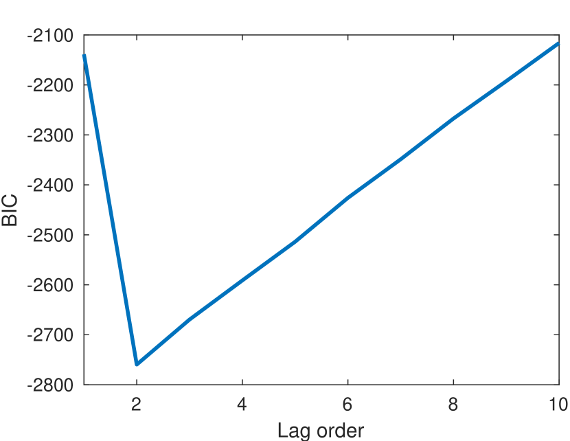
(a) BIC

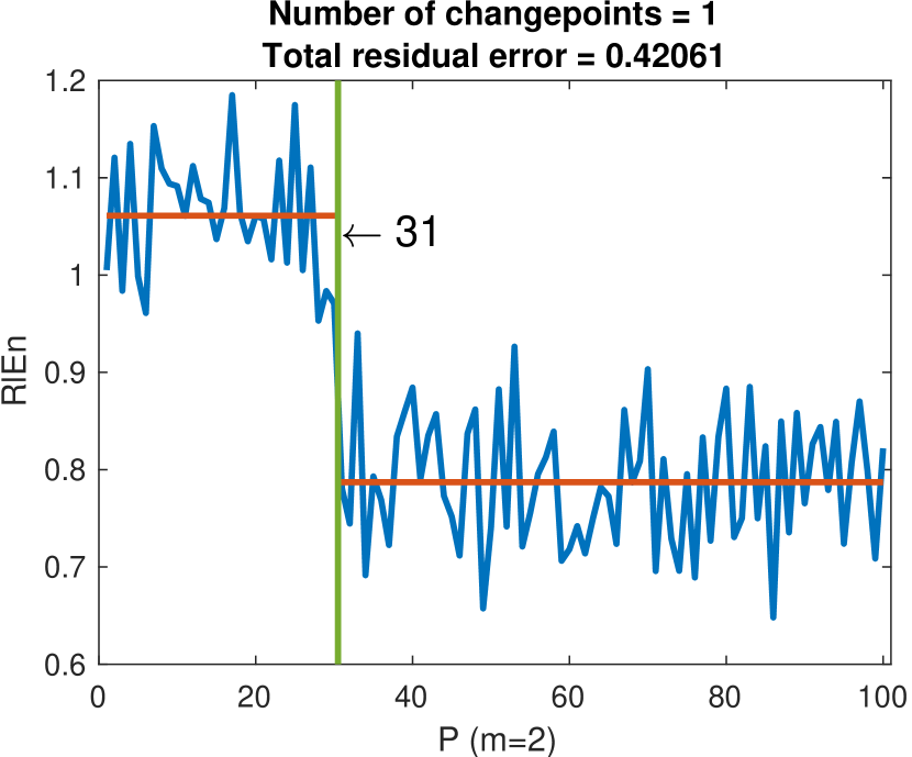
(b) Change-point

Figure 6: Result of Case 1

References

- Acharya U. et al. (2005) Acharya U., R., O. Faust, N. Kannathal, T. Chua, and S. Laxminarayan (2005). Non-linear analysis of EEG signals at various sleep stages. Computer Methods and Programs in Biomedicine 80(1), 37–45.
- Acharya U et al. (2004) Acharya U, R., K. N, O. W. Sing, L. Y. Ping, and T. Chua (2004). Heart rate analysis in normal subjects of various age groups. BioMedical Engineering OnLine 3, 24.
- Braun et al. (2000) Braun, J. V., R. K. Braun, and H. G. Muller (2000). Multiple Changepoint Fitting via Quasilikelihood, with Application to DNA Sequence Segmentation. Biometrika 87(2), 301–314.
- Brown (1971) Brown, B. M. (1971). Martingale Central Limit Theorems. The Annals of Mathematical Statistics 42(1), 59–66.
- Burioka et al. (2005) Burioka, N., M. Miyata, G. Cornélissen, F. Halberg, T. Takeshima, D. T. Kaplan, H. Suyama, M. Endo, Y. Maegaki, T. Nomura, Y. Tomita, K. Nakashima, and E. Shimizu (2005). Approximate entropy in the electroencephalogram during wake and sleep. Clinical EEG and neuroscience 36(1), 21–24.
- Butterworth (1930) Butterworth, S. (1930). On the Theory of Filter Amplifiers. Experimental Wireless and the Wireless Engineer 7, 536–541.
- Chen (1999) Chen, S. X. (1999). Beta kernel estimators for density functions. Computational Statistics & Data Analysis 31(2), 131–145.
- Chen et al. (2009) Chen, W., J. Zhuang, W. Yu, and Z. Wang (2009). Measuring complexity using FuzzyEn, ApEn, and SampEn. Medical Engineering & Physics 31(1), 61–68.
- Costa et al. (2003) Costa, M., C. K. Peng, A. L. Goldberger, and J. M. Hausdorff (2003). Multiscale entropy analysis of human gait dynamics. Physica A: Statistical Mechanics and its Applications 330(1), 53–60.
- Dickey and Fuller (1981) Dickey, D. A. and W. A. Fuller (1981). Likelihood ratio statistics for autoregressive time series with a unit root. Econometrica 49(4), 1057–1072.
- Fan and Yao (2003) Fan, J. and Q. Yao (2003). Nonlinear Time Series: Nonparametric and Parametric Methods. Springer Series in Statistics. New York: Springer-Verlag. Literaturverz. [487] - 536.
- Forrest et al. (2014) Forrest, S. M., J. H. Challis, and S. L. Winter (2014). The effect of signal acquisition and processing choices on ApEn values: Towards a “gold standard” for distinguishing effort levels from isometric force records. Medical Engineering & Physics 36(6), 676–683.
- Fryzlewicz (2014) Fryzlewicz, P. (2014). Wild binary segmentation for multiple change-point detection. The Annals of Statistics 42(6), 2243–2281.
- Hall (1988) Hall, P. (1988). Estimating the direction in which a data set is most interesting. Probability Theory and Related Fields 80(1), 51–77.
- Hall et al. (2004) Hall, P., J. Racine, and Q. Li (2004). Cross-Validation and the Estimation of Conditional Probability Densities. Journal of the American Statistical Association 99(468), 1015–1026.
- Härdle (1990) Härdle, W. (1990). Applied Nonparametric Regression. Cambridge University Press.
- Hong and White (2005) Hong, Y. and H. White (2005). Asymptotic Distribution Theory for Nonparametric Entropy Measures of Serial Dependence. Econometrica 73(3), 837–901.
- Hyndman and Athanasopoulos (2013) Hyndman, R. J. and G. Athanasopoulos (2013). Forecasting: Principles and Practice. OTexts.
- Ihara (1993) Ihara, S. (1993). Information Theory for Continuous Systems. World Scientific.
- Inclán and Tiao (1994) Inclán, C. and G. C. Tiao (1994). Use of Cumulative Sums of Squares for Retrospective Detection of Changes of Variance. Journal of the American Statistical Association 89(427), 913–923.
- John (1984) John, R. (1984). Boundary modification for kernel regression. Communications in Statistics - Theory and Methods 13(7), 893–900.
- Jones (1993) Jones, M. C. (1993). Simple boundary correction for kernel density estimation. Statistics and Computing 3(3), 135–146.
- Killick et al. (2012) Killick, R., P. Fearnhead, and I. A. Eckley (2012). Optimal Detection of Changepoints With a Linear Computational Cost. Journal of the American Statistical Association 107(500), 1590–1598.
- Kullback and Leibler (1951) Kullback, S. and R. A. Leibler (1951). On information and sufficiency. The Annals of Mathematical Statistics 22(1), 79–86.
- Li et al. (2024) Li, J., P. Fearnhead, P. Fryzlewicz, and T. Wang (2024, 01). Automatic change-point detection in time series via deep learning. Journal of the Royal Statistical Society Series B: Statistical Methodology 86(2), 273–285.
- Li et al. (2024) Li, J., R. Ma, M. Deng, X. Cao, X. Wang, and X. Wang (2024). A comparative study of clustering algorithms for intermittent heating demand considering time series. Applied Energy 353, 122046.
- Li and Racine (2007) Li, Q. and J. S. Racine (2007). Nonparametric Econometrics: Theory and Practice. Princeton, N.J: Princeton University Press.
- Marron and Ruppert (1994) Marron, J. S. and D. Ruppert (1994). Transformations to reduce boundary bias in kernel density estimation. Journal of the Royal Statistical Society: Series B (Methodological) 56(4), 653–671.
- Page (1954) Page, E. S. (1954). Continuous inspection schemes. Biometrika 41(1-2), 100–115.
- Pethick et al. (2016) Pethick, J., S. L. Winter, and M. Burnley (2016). Loss of knee extensor torque complexity during fatiguing isometric muscle contractions occurs exclusively above the critical torque. American Journal of Physiology-Regulatory, Integrative and Comparative Physiology 310(11), R1144–R1153.
- Picard et al. (2011) Picard, F., E. Lebarbier, M. Hoebeke, G. Rigaill, B. Thiam, and S. Robin (2011). Joint segmentation, calling, and normalization of multiple CGH profiles. Biostatistics (Oxford, England) 12(3), 413–428.
- Pincus (1991) Pincus, S. M. (1991). Approximate entropy as a measure of system complexity. Proceedings of the National Academy of Sciences 88(6), 2297–2301.
- Richman and Moorman (2000) Richman, J. S. and J. R. Moorman (2000). Physiological time-series analysis using approximate entropy and sample entropy. American Journal of Physiology-Heart and Circulatory Physiology 278(6), H2039–H2049.
- Robinson (1991) Robinson, P. M. (1991). Consistent Nonparametric Entropy-Based Testing. The Review of Economic Studies 58(3), 437–453.
- Roussas and Ioannides (1988) Roussas, GG. and D. Ioannides (1988). Probability bounds for sums in triangular arrays of random variables under mixing conditions. Statistical Theory and Data Analysis II, 293–308.
- Schuster (1985) Schuster, E. F. (1985). Incorporating support constraints into nonparametric estimators of densities. Communications in Statistics - Theory and Methods 14(5), 1123–1136.
- Shao (1997) Shao, J. (1997). An Asymptotic Theory for Linear Model Selection. Statistica Sinica 7(2), 221–242.
- Shi et al. (2017) Shi, B., Y. Zhang, C. Yuan, S. Wang, and P. Li (2017). Entropy Analysis of Short-Term Heartbeat Interval Time Series during Regular Walking. Entropy 19(10), 568.
- Shibata (1981) Shibata, R. (1981). An Optimal Selection of Regression Variables. Biometrika 68(1), 45–54.
- Vieu (1991) Vieu, P. (1991). Smoothing Techniques in Time Series Analysis. In G. Roussas (Ed.), Nonparametric Functional Estimation and Related Topics, NATO ASI Series, pp. 271–283. Dordrecht: Springer Netherlands.
- Vieu (1995) Vieu, P. (1995). Order Choice in Nonlinear Autoregressive Models. Statistics 26(4), 307–328.
- Wakeman and Henson (2015) Wakeman, D. G. and R. N. Henson (2015). A multi-subject, multi-modal human neuroimaging dataset. Scientific Data 2(1), 150001.
- Wang and Samworth (2017) Wang, T. and R. J. Samworth (2017, 08). High dimensional change point estimation via sparse projection. Journal of the Royal Statistical Society Series B: Statistical Methodology 80(1), 57–83.
- Wasserman (2006) Wasserman, L. (2006). All of Nonparametric Statistics. Springer Texts in Statistics. New York: Springer.