HotSpot: Screened Poisson Equation for Signed Distance Function Optimization

Abstract

We propose a method, HotSpot, for optimizing neural signed distance functions, based on a relation between the solution of a screened Poisson equation and the distance function. Existing losses such as the eikonal loss cannot guarantee the recovered implicit function to be a distance function, even when the implicit function satisfies the eikonal equation almost everywhere. Furthermore, the eikonal loss suffers from stability issues in optimization and the remedies that introduce area or divergence minimization can lead to oversmoothing. We address these challenges by designing a loss function that when minimized can converge to the true distance function, is stable, and naturally penalize large surface area. We provide theoretical analysis and experiments on both challenging 2D and 3D datasets and show that our method provide better surface reconstruction and more accurate distance approximation.

Figure 1: We propose HotSpot, a neural signed distance function optimization method that can obtain accurate signed distance function for complex shapes. Here we show a reconstruction from a point cloud sampled from the reference bunny (taken from Mehta et al. [1]) on the right. In the inset, we visualize the recovered signed distance function on a horizontal slice, using warm colors for positive values and cold for negative (zoom in for details). Our reconstruction is significantly more accurate than prior works (SAL [2], DiGS [3], and StEik [4]).

1 Introduction

Learning neural signed distance function requires designing loss functions so that the zero crossings of the implicit function is at the desired locations (e.g., adhere to a sparse input point cloud), and that the implicit function returns correct signed distance. The design of the loss proves to be challenging for shapes with complex topology and details (Fig. 1). We propose HotSpot, a method based on a relation between screened Poisson equation and distance that enjoys both theoretical and practical benefits.

A major challenge of signed distance function optimization is to ensure that the implicit function indeed outputs the signed distance. A standard regularization loss used is the eikonal equation: it constrains the norm of the gradient of an implicit function to be $1$ almost everywhere. If the implicit function is a signed distance function, then it satisfies the eikonal equation. However, the converse is not true. Fig. 2 shows an example: on the left, we optimize an implicit function to satisfy the eikonal equation, while it successfully does so, it converges to a solution that is far from the actual distance [5, 6].

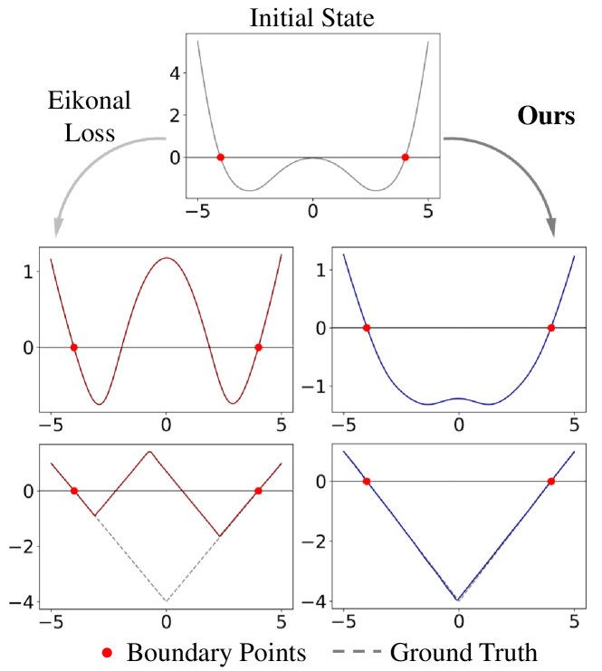
Figure 2: We illustrate an 1D neural signed distance function optimization using the classical eikonal loss [7] and our model. The $x$ axis is the domain and the $y$ axis shows the output of the impilcit function. The gray dashed line is the reference signed distance function. The middle and bottom rows show the intermediate and final states of the optimization respectively. The eikonal loss is incapable of converging to the actual signed distance function (dashed line), even when the function satisfies the eikonal equation almost everywhere. Our method converges to the ground truth by modeling a screened Poisson equation.

Another key challenge lies in the optimization. It is known that the eikonal equation regularization is unstable [4], and the instability can make optimization converge to suboptimal results or even diverge. Furthermore, to combat both the ill-posedness and the instability of the optimization, existing methods need to penalize the surface area of the shape, which leads to a delicate balance between over- and under-smoothing.

We propose a simple model that can be used together with the eikonal equation to address all the challenges above. Our model, HotSpot, is based on a screened Poisson equation and a classical relation between heat transfer and distance [8], that was popular for approximating both Euclidean and geodesic distance [9, 10]. Using this relation, we design a loss function for optimizing neural signed distance functions. As our contributions, we show, both theoretically and empirically, that our model

• has a bounded difference from the actual distance and can converge to it (Fig. 2, right).

• is stable both spatially and temporally, in the sense that a slight perturbation of the implicit function only introduce changes in a local region, and that the dynamical system formed by the gradient flow will converge in the long run.

• penalizes the surface area naturally, while being compatible with being a signed distance function.

• works well in both 2D and 3D shapes, and it excels at approaching the signed distance functions while optimizing for complex, high genus shapes.

2 Related Work

Implicit surfaces. Modeling and reconstructing surfaces using implicit functions has a long history in computer vision and graphics [11, 12, 13, 14, 15]. Recently, there is a surge of interests to model surfaces using neural implicit functions [16, 17, 18, 19, 20]. Neural implicit representations are favored for their compactness, ability to represent highly-detailed surfaces, and compatibility to gradient-based optimization [1].

Neural signed distance functions. Among the classes of implicit surfaces, signed distance functions, where the implicit function outputs the distance to the closest point on the surface, and the sign represents whether the point is inside or outside the solid object, is one of the most popular variants. Signed distance functions enable an efficient rendering algorithm called sphere tracing [21, 22, 23, 24] and helps geometry compression [25]. They can also be used for collision detection [26, 27, 28], and numerical simulation [29]. Traditionally, signed distance functions are often represented as grids [6]. More recently, neural signed distance functions have become an appealing geometric representation [30, 31, 32]. (Neural) Signed distance functions are also often used in inverse rendering [33, 34, 35, 36, 37, 38, 39], for their flexibility to obtain surfaces with complex topology.

Regularizing and initializing neural signed distance functions. A commonly used loss for optimizing neural signed distance functions is the eikonal regularization, which encourages the norm of the gradient of the implicit function to be one [7, 36]. However, the eikonal regularization alone is far from sufficient, as 1) it can contain many undesirable local minima [4], and 2) minimizing eikonal loss does not necessarily lead to a distance field [5, 6]. Previous works have proposed initialization to bootstrap the optimization with a simple shape [7, 3]. Recent works show that minimizing the divergence and the surface area of the implicit function can lead to better reconstruction [3, 40, 41] and stabilizes the optimization [4]. Second-order information is also often used [41, 42] for regularization. Specialized architectures have been proposed for limiting the Lipchitz constant of the implicit function [32] and for representing high-frequency details [31, 25, 43]. Lipman [44] showed a connection between the regularization of occupancy function optimization and an approximated signed distance field using the phase transition theory of fluids.

We propose a new loss and method for optimizing signed distance functions. While derived from very different mathematics, our loss turns out to have a close connection to Lipman’s PHASE loss. We show that our theory leads to significantly more numerically stable optimization, and a different conclusion in the parameter setting that leads to drastically different results.

Distance approximation using heat transfer. Our derivation is inspired by a relation between heat transfer and approximated distance [8]. This relation has been used in computer graphics for efficiently computing the geodesic distance on surfaces [9, 10, 45, 46]. We apply the relation for optimizing neural signed distance functions, and analyze the properties of the resulting optimization in this context.

3 Background and Motivation

Given an input point cloud $\bm{x}_{i}\in\mathbb{R}^{d}$ (we focus on 2D and 3D in this work) with $N$ points without normal information that lies on an unknown surface $\Gamma$ of a solid object $S$, our goal is to find a signed distance function $f(\bm{x})$, such that

$$f(\bm{x})=\begin{cases}-d_{\Gamma}(\bm{x})&\text{ if }\bm{x}\in S\\ d_{\Gamma}(\bm{x})&\text{ otherwise, }\end{cases}$$ (1)

where $d_{\Gamma}(\bm{x})$ denotes the closest distance from point $\bm{x}$ to the surface $\Gamma$. In practice, we approximate the signed distance function $f(\bm{x})$ using a neural network $u(\bm{x}):\mathbb{R}^{d}\rightarrow\mathbb{R}$ parameterized by its weights and use gradient-based optimization to figure out the weights. Previous work (e.g., [7]) often uses a linear combination of a boundary loss $L_{\text{boundary}}$ and a eikonal loss $L_{\text{eikonal}}$:

$$L_{\text{boundary}} =\frac{1}{N}\sum_{i=1}^{N}\left|u(\bm{x}_{i})\right|^{p},$$ (2)

$$L_{\text{eikonal}} =\int_{\Omega}\left|\left\|\nabla u(\bm{x})\right\|-1\right|^{p}\,\mathrm{d}\bm{x},\quad p=1\,\text{or}\,2,$$ (3)

where $\Omega\subset\mathbb{R}^{d}$ is our domain of interest. The boundary loss encourages the implicit function $u$ to output $0$ at the boundary, and the eikonal loss is based on that observation that if a function $f$ is a distance function, the $L^{2}$ norm of its gradient $\left\|\nabla f(\bm{x})\right\|=1$ holds almost everywhere. Thus the approximation $u$ is encouraged to behave the same.

However, as mentioned earlier, simply optimizing for the two terms above can lead to unsatisfactory results, as the eikonal loss does not guarantee that $u$ would be a distance function even when satisfied almost everywhere (Fig. 2), and the extra regularization previous work added to minimize the area and divergence [3, 4] could further tamper with the distance approximation quality. We derive an additional loss that can be used together with both of the losses above, and analyze our loss theoretically and empirically.

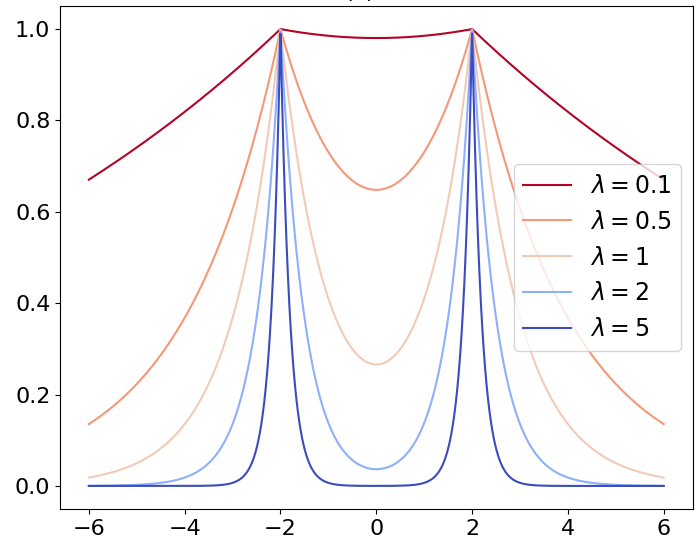
(a) 1D Screened Poisson Equation

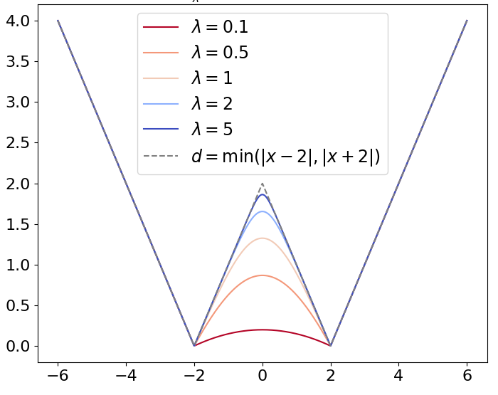
(b) Distance Reconstruction

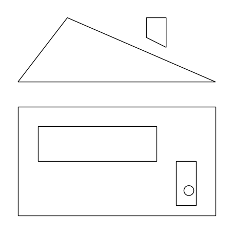
(c) House

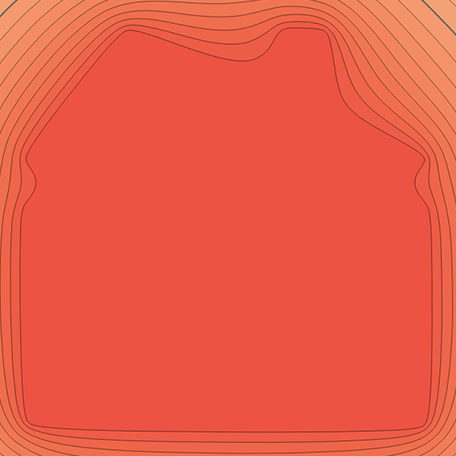
(d) $\lambda=1$

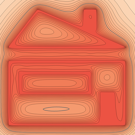
(e) $\lambda=5$

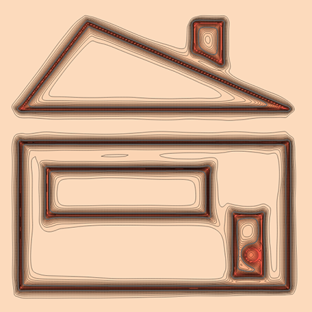
(f) $\lambda=50$

Figure 3: We show an illustration of the relation between screened Poisson equation and a distance field. The top shows an 1D example, where on the left we show a solution to Eq. 4 with different absorption $\lambda$, and on the right we show the reconstructed distance $\frac{1}{\lambda}\ln(h)$ (Eq. 5). As $\lambda$ increases, the heat cools down faster, and the reconstructed function approaches the real distance. The bottom shows a 2D example.

We will be using a key relation between the screen Poisson equation and the distance. We first define a screened Poisson equation over a heat field $h(\bm{x}):\mathbb{R}^{d}\rightarrow\mathbb{R}$, with an absorption coefficient $\lambda$, and set a Dirichlet boundary condition to be $1$ on our target surface $\Gamma$:

$$\left\{\begin{aligned} &\nabla^{2}h(\bm{x})-\lambda^{2}h(\bm{x})=0\quad\forall\bm{x}\in\mathbb{R}^{d}\setminus\Gamma\\ &\lim_{||\bm{x}||\to\infty}h(\bm{x})=0,\quad h(\bm{x})=1\quad\forall\bm{x}\in\Gamma.\end{aligned}\right.$$ (4)

If a heat field $h_{\lambda}$ is a solution to the partial differential equation above, then the following equation holds [8]:

$$\lim_{\lambda\to\infty}\frac{1}{\lambda}\ln(h_{\lambda}(\bm{x}))=-d_{\Gamma}(\bm{x}).$$ (5)

Fig. 3 shows the intuition. Screened Poisson equation simulates heat transfer until an equilibrium is reached, under absorption controlled by the $\lambda$ coefficient. As we increase the absorption, the reconstructed distance $\frac{1}{\lambda}\ln(h_{\lambda})$ would approach the real distance. In practice, we could only obtain a discrete point set $\Gamma_{0}$. Provided that the neighbor points are close enough, if there are some boundaries connecting them, the boundary condition of Eq. 4 still holds. This can be interpreted as a superset $\Gamma$ replacing $\Gamma_{0}$, effectively transforming the boundary from a discrete point cloud into a continuous surface, which is required and precisely the goal in the signed distance function reconstruction. The reconstructed distance can still faithfully represent the distance to $\Gamma$ because the approximation in Eq. 5 still holds. We will later prove that the measure of $\Gamma$ is bounded by our loss.

4 Method

In this section, we introduce our method, HotSpot, based on the screened Poisson equation (Eq. 4) and derive theoretical analysis. We use the screened Poisson equation to derive a loss we can directly apply to an implicit function $u$, and prove that there is a bound to the solution of the screened Poisson equation to the true distance (Section 4.1). We further derive stability analysis of our loss on both the spatial stability over small perturbation and the temporal convergence (Section 4.2). Next, we show that our loss can penalize surfaces with large area (Section 4.3). Finally, we discuss the relation to a prior work, PHASE (Section 4.4).

4.1 Screened Poisson Equation Informed Signed Distance Functions Optimization

Given an implicit function $u$, we want to derive a loss based on the screened Poisson equation (Eq. 4) and its relation to the distance (Eq. 5). We achieve this by applying the following substitution based on Eq. 5:

$$h(\bm{x})=e^{-\lambda|u(\bm{x})|}.$$ (6)

We want to design a loss such that its minimizer would satisfy the screened Poisson equation. This can be achieved by minimizing the energy functional $\frac{1}{2}\int_{\Omega}\|\nabla h(\bm{x})\|^{2}+\lambda^{2}h(\bm{x})^{2}\,\mathrm{d}\bm{x}$. After substitution and removal of the constant factor $\lambda$, we obtain our heat loss:

$$L_{\text{heat}}=\frac{1}{2}\int_{\Omega}e^{-2\lambda|u(\bm{x})|}\left(\|\nabla u(\bm{x})\|^{2}+1\right)\,\mathrm{d}\bm{x}.$$ (7)

If we take the derivative of $L_{\text{heat}}$ with respect to the heat field $h$, we can see that it recovers the screened Poisson equation $\nabla^{2}h-\lambda^{2}h=0$. The boundary condition can be enforced by the standard boundary loss (Eq. 2), by observing that $u(\bm{x})=0$ implies $h(\bm{x})=1$. Together with the eikonal loss, we optimize:

$$L=w_{b}L_{\text{boundary}}+w_{e}L_{\text{eikonal}}+w_{h}L_{\text{heat}}.$$ (8)

While prior work [8] has studied the limiting behavior of the absorption coefficient $\lambda$, to our knowledge, the bounds of the approximation and the convergence speed remains unknown. In the supplementary material A.3, we prove that, for a boundary $\Gamma$ formed by a discrete set of points and a small volume around them, the distance approximation obtained from the solution of the screened Poisson equation converges linearly with respect to $\lambda$:

$$\frac{1}{\lambda}C_{\text{lower}}(\bm{x})\leqslant\frac{1}{\lambda}\ln(h_{\lambda}(\bm{x}))+d_{\Gamma}(\bm{x})\leqslant\frac{1}{\lambda}C_{\text{upper}}(\bm{x}).$$ (9)

Here, both $C_{\text{upper}}(\bm{x})$ and $C_{\text{lower}}(\bm{x})$ are scalar fields independent to $\lambda$. The inequalities are tight, which means that one can find a case where the equality holds.

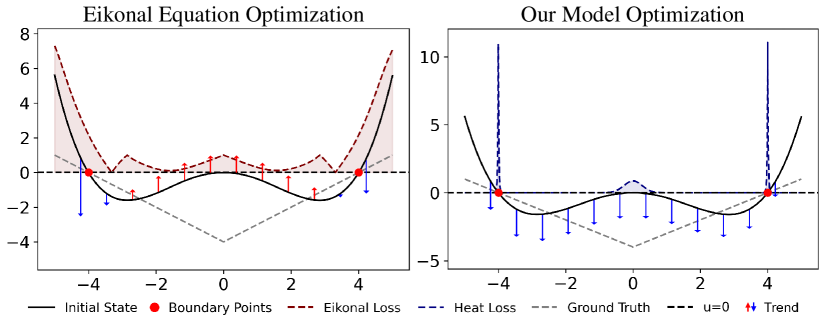
Figure 4: We visualize the direction of the changes of the implicit function during one iteration of optimization. Left shows the result with only the eikonal loss and right shows the result after adding our loss. Our loss avoids the local minimum in Fig. 2.

Compared to the eikonal loss (Eq. 3), where the error to the actual distance can be unbounded even when the implicit function satisfies the eikonal equation almost everywhere, Eq. 9 highlights the fact that even with a finite absorption $\lambda$, our loss can lead to much more accurate distance. In fact, any loss that only depends on the norm of the gradients $\left\|\nabla u\right\|$ would be incapable of distinguishing between a pseudo signed distance function [5] and an actual one, due to the discontinuous jumps of the gradient. Adding our loss (Eq. 7) ensures that the implicit function converges to the actual signed distance. Fig. 4 visualizes the direction of how an implicit function would evolve for only using the eikonal loss and after adding our loss. Our loss ensures that the implicit function evolves towards the direction of the actual distance.

4.2 Stability Analysis

Our heat loss enjoys other theoretical benefits apart from the convergence to an actual distance. Here, we show that our loss leads to easier optimization. We separately analyze spatial stability and temporal stability, where the spatial stability studies the effect of small perturbation error added to the corresponding partial differential equation, and the temporal stability studies the convergence of the gradient flow.

4.2.1 Spatial Stability

We show that for the screened Poisson equation, an error introduces to a single point in the solution decays exponentially and do not propagate to infinitely distant positions. On the contrary, for the corresponding partial differential equation formed by the eikonal equation, the error can propagate to infinitely far away. The property of the screened Poisson equation ensures that the perturbation we introduce during optimization does not lead to a drastically different target and stablizes the optimization.

First, we show that for the partial differential equation formed by the eikonal equation, an additive error introduced to a point can preserve along a line segment or a ray.

Proposition 1.

Given a field $u(\bm{x})$ that satisfies the eikonal equation $\left\|\nabla u\right\|=1$, we introduce an additive error $u_{0e}$ at the point $\bm{x}_{0}$ where $u(\bm{x}_{0})=u_{0}$ to obtain a perturbed field $u^{\prime}$ where $u^{\prime}(\bm{x}_{0})=u_{0}+u_{0e}$ and $\left\|\nabla u^{\prime}\right\|=1$. In the perturbed field $u^{\prime}$, there exists a line segment parameterized by $\bm{x}(s)$ starting from $\bm{x}_{0}$ and $s\in[0,M]$, where $M>0$ and can be infinite, such that every point along the line has the same error:

$$u^{\prime}(\bm{x}(s))-u(\bm{x}(s))=u_{0e}$$ (10)

The boundary points can contain errors when approximating the true boundaries, and these errors remain constant along the line segment. As a result, the propagated error can become significant and potentially detrimental.

Next, we demonstrate that the error field $h_{e}$ in Eq. 4 decays exponentially from the perturbed point $\bm{x}_{0}$.

Proposition 2.

In 3D space, consider an additive error $h_{0e}$ within a small ball $B(\bm{x_{0}},\epsilon)$ around the point $\bm{x_{0}}$, where the original field $h(\bm{x})$ and the perturbed field $h^{\prime}(\bm{x}),\,\bm{x}\in\mathbb{R}^{n}\setminus B$ both satisfy the screened Poisson equation in Eq. 4. The resulting error field $h_{e}=h^{\prime}-h$ is radially symmetric with respect to $\bm{x}_{0}$ within some maximum radius $R$, and is given by

$$h_{e}(r)=\frac{\epsilon}{r}h_{0e}e^{\lambda(\epsilon-r)},\,\forall r>\epsilon,$$ (11)

where $r=\|\bm{x}-\bm{x_{0}}\|$ is the radial distance from $\bm{x_{0}}$.

The proofs of these two propositions are in the supplementary material A.1 and A.2. By comparing the error fields, we observe that the partial differentiation equation governed by the screened Poisson equation exhibits greater spatial robustness than the one based on eikonal equation.

4.2.2 Temporal Stability

We next demonstrate the temporal stability of the heat loss and show that the dynamical system of the gradient update is stable, that is, the solution of the dynamical system would converge as the time $t$ approaches infinity. This analysis is supported by von Neumann stability analysis, similar to Yang et al.’s work [4].

Yang et al. showed that for the eikonal loss (Eq. 3), the temporal gradient flow of the optimization is:

$$\frac{\partial u}{\partial t} =-\frac{\delta L_{\text{eikonal}}}{\delta u}=\nabla\cdot(\kappa_{e}\nabla u)\approx\kappa_{e}\nabla^{2}u,\,\text{where}$$ (12)

$$\kappa_{e}(\bm{x}) =\left\{\begin{array}[]{ll}\frac{1}{|\nabla u(\bm{x})|}\operatorname{sgn}(|\nabla u(\bm{x})|-1)&p=1\\ 1-|\nabla u(\bm{x})|^{-1}&p=2\end{array}\right.$$

They analyze the stability by applying Fourier transform to both sides:

$$\frac{\partial\hat{u}}{\partial t}(t,\omega)=-\kappa_{e}|\omega|^{2}\hat{u}(t,\omega)\Rightarrow\hat{u}(t,\omega)\propto e^{-\kappa_{e}|\omega|^{2}t},$$ (13)

where $\omega=(\omega_{1},\dots,\omega_{n})$ denotes the frequency variable and $\hat{u}$ represents the Fourier transform of $u$. In the frequency domain, if the original function converges, the term $\frac{\partial\hat{u}}{\partial t}$ should also converge. However, when $\kappa_{e}<0$, this process corresponds to backward diffusion, which diverges and is inherently unstable regardless of the numerical implementation.

We extend the analysis to our heat loss (Eq. 7). The gradient flow is

$$\frac{\partial h}{\partial t}=-\frac{\delta L_{\text{heat}}}{\delta h}=\nabla^{2}h-\lambda^{2}h$$ (14)

This is exactly the heat equation, and is known to be stable. We can further verify the stability by applying Fourier transform to both sides:

$$\frac{\partial\hat{h}}{\partial t}(t,\omega)=-(|\omega|^{2}+\lambda^{2})\hat{h}(t,\omega)\Rightarrow\hat{h}(t,\omega)\propto e^{-(|\omega|^{2}+\lambda^{2})t}$$ (15)

This analysis reveals that the original process $h(\bm{x},t)$ converges over time and remains stable. Due to the constraint $|u|=-\ln(h)/\lambda$, the term $|u(\bm{x},t)|$ also converges during the optimization process. Since $u$ is continuous, it converges as well.

Based on this analysis, we have demonstrated that our method exhibits greater stability compared to the eikonal equation in both the spatial and temporal domains.

4.3 Surface Area Regularization

We next show that our heat loss (Eq. 7) penalizes large area of the reconstructed surfaces, by showing its relation to the coarea loss used by Pumarola et al. [6]. Pumarola et al. showed that the loss $\int_{\Omega}e^{-\lambda|u|}\|\nabla u\|\,\mathrm{d}\bm{x}$ approximates the surface area of the zero level set of the implicit function $u$. We then form the following inequality:

$$\begin{split}\int_{\Omega}e^{-\lambda|u|}\|\nabla u\|\,d\bm{x}&<\int_{\Omega}\sqrt{e^{-2\lambda|u|}({\|\nabla u\|}^{2}+1)}\,d\bm{x}\\ \leqslant\sqrt{|\Omega|}&\cdot\sqrt{\int_{\Omega}e^{-2\lambda|u|}({\|\nabla u\|}^{2}+1)\,d\bm{x}}\end{split}$$ (16)

Therefore, minimizing the right hand side (our heat loss) leads to a reduction in the upper bound of the left hand side.

Furthermore, we can show that the coarea loss is too aggressive for our purpose of signed distance field reconstruction. If we directly minimize the coarea loss (the left hand side in Eq. 16) by applying the Euler-Lagrange equation, the minimizer would satisfy:

$$1-\frac{\nabla^{2}u}{\|\nabla u\|}=0,$$ (17)

which does not relate to the regularization parameter $\lambda$. Unfortunately, the partial differential equation system formed by the equation above and the eikonal equation does not have a solution in general. We can see this by plugging in $\|\nabla u\|=1$ to get a Poisson’s equation $\nabla^{2}u=1$. Under certain boundary condition, it has a unique solution of the gradient $\nabla u$, while the gradient is not guaranteed to have a unit norm. This makes the coarea loss unable to accurately represent a signed distance function. By contrast, our heat loss has bounds for its distance approximation and converges to the true distance as we increase the parameter $\lambda$ (Eq. 9).

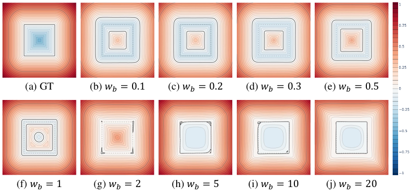
Figure 5: We reproduce the PHASE model [44] and show the log-transformed occupancy field, i.e., the optimized signed distance function. PHASE recommends boundary weight range $w_{b}\in\left(0.10,0.32\right)$ based on their $\Gamma$-convergence theory. But in practice, only a stronger boundary weight constrains the boundary to follow the input points. We found that this phenomenon often occurs and show more examples in the supplementary material.

4.4 Relation to PHASE [44]

While derived from very different mathematical principles and a different motivation, our method has a close relation to the PHASE model proposed by Lipman. PHASE is motivated by smoothly approximating an occupancy function $o(\bm{x})$, which outputs $1$ outside the object, $-1$ inside, and $0$ on the surface.

In the supplementary material, we show that there is a close relation between our heat field $h$ and the smoothed occupancy function $o$. We further show that our theory and derivation have led to additional insights and significant differences in implementation and results. In particular, PHASE’s theory introduces a condition stating that the boundary loss weight $w_{b}$ should be small, whereas our theory emphasizes the need for a firm boundary condition (Eq. 4 and Fig. 5).

Furthermore, we found that optimizing occupancy field in the PHASE model can be numerically unstable when the regularized occupancy $o$ approaches $1$ or $-1$. When used together with the eikonal loss, it can lead to unbounded network weight derivatives, impeding the optimization. Optimizing directly for the signed distance function like in our method avoids this issue.

5 Experiments

We show experiments on both 2D and 3D datasets. We construct a 2D dataset containing 14 shapes, ranging from simple geometric shapes to complex nested strctures. We also evaluate on two 3D benchmarks: a subset of ShapeNet [47] and the Surface Reconstruction Benchmark (SRB) [48]. Additionally, we generate a dataset with high genus geometries from Mehta et al. [1]. In all of our experiments, we use only the position information of the point cloud.

We report the Intersection over Union (IoU), Chamfer distance, and Hausdorff distance between reconstructed shapes and ground truth shapes as metrics for surface reconstruction. In addition, we report Root Mean Squared Error (RMSE), Mean Absolute Error (MAE), and Symmetric Mean Absolute Percentage Error (SMAPE) as metrics for distance field evaluation. We further evaluate non-zero level set quality near the surface, and render the zero level set of the signed distance functions via sphere tracing.

We use a network with 5 hidden layers and 128 hidden channels for our method in all experiments. The hyperparameters are consistent within each dataset. To sample the integrals of our loss, we apply importance sampling to accurately estimate the heat loss integral. Full training details can be found in the supplementary material.

5.1 2D Dataset

An overview of our 2D dataset is attached in the supplementary material. For 2D experiments, we simply use a linear network and geometric initialization, as in DiGS [3]. We compare our method with DiGS [3] and StEik [4] with the hyperparameters and training configuration provided in their released code, and report the surface reconstruction metrics and distance field metrics in Table 2. Our method outperforms theirs across all metrics with only 8,192 sample points, whereas both of the previous methods use 15,000 sample points based on their default settings.

5.2 Ablation Study on 2D Dataset

To more comprehensively compare over different losses, we conduct an ablation study on our 2D dataset using the same network architecture, parameter initialization, and sampling strategy. The only difference lies in the loss functions used. Quantitative results are shown in Table 2.

The last row corresponds to our HotSpot model, which uses a combination of boundary, eikonal, and heat losses. Our method reconstructs the correct topology for all 14 shapes, while others struggle with the harder ones. It outperforms across nearly all metrics, demonstrating superior reconstruction quality and distance query accuracy. Although HotSpot slightly lags behind SAL [49] in RMSE and MAE, it successfully captures the correct topology for complex shapes, while SAL fails to do so. A visualization is shown in Fig. 6. Full qualitative results and detailed experiment parameters are provided in the supplementary material. Models relying heavily on area losses [3, 4] often face a trade-off between preserving original details and eliminating excess boundaries, which distorts the distance field (Section 4.3). Moreover, methods without our heat loss fall in local optimum easily.

	IoU $\uparrow$	$d_{C}$ $\downarrow$	$d_{H}$ $\downarrow$
DiGS [3]	0.7882	0.0055	0.1267
StEik [4]	0.6620	0.0073	0.1425
Ours	0.9870	0.0014	0.0153
	RMSE $\downarrow$	MAE $\downarrow$	SMAPE $\downarrow$
DiGS [3]	0.0597	0.0315	0.3363
StEik [4]	0.0725	0.0419	0.4222
Ours	0.0199	0.0101	0.0699

Table 1: Comparison of 2D reconstruction and distance query. $d_{C}$ and $d_{H}$ stand for the Chamfer and Hausdorff distances respectively. Our method outperforms DiGS [3] and StEik [4] on all metrics.

$\mathcal{L}_{B}$	$\mathcal{L}_{E}$	$\mathcal{L}_{A}$	$\mathcal{L}_{D}$	$\mathcal{L}_{DD}$	$\mathcal{L}_{S}$	$\mathcal{L}_{H}$	IoU	$d_{C}$	$d_{H}$	RMSE	MAE	SMAPE
✓	✓						0.8192	0.0068	0.0712	0.0377	0.0158	0.1315
✓					✓		0.8936	0.0029	0.0579	0.0165	0.0081	0.1205
✓	✓		✓				0.3907	0.0843	0.5598	0.2966	0.2388	1.7283
✓	✓	✓	✓				0.6338	0.0566	0.4221	0.2058	0.1616	1.0919
✓	✓			✓			0.2938	0.0377	0.3444	0.2990	0.2355	1.6958
✓	✓	✓		✓			0.6037	0.0414	0.3656	0.1304	0.0937	0.7792
✓	✓					✓	0.9851	0.0016	0.0160	0.0199	0.0105	0.0754

Table 2: Ablation study of different loss combinations and metrics. From top to bottom, the loss combinations are from: IGR [7], SAL [49], DiGS w/o area loss, DiGS [3], StEik w/o loss, StEik [4], and our HotSpot. From left to right, the losses are boundary loss, eikonal loss, area loss, divergence loss, directional divergence loss, SAL loss, heat loss.

Figure 6: Our heat loss achieves the best reconstruction of triangle fragments. Dashed lines show real boundaries, while the boldest line represents reconstructed ones. (c) and (f) are from the original models by DiGS [3] and StEik [4]; the rest are from our ablation study with different loss combinations. Other combinations fail to remove extra boundaries or accurately capture the topology. More fundamentally, (c), (f), (g), and (h) fall into local optima, leading to incorrect depressions and elevations.

5.3 3D Datasets

We evaluate our method on a processed subset [19, 16, 50] of ShapeNet [47], which provides surface point sampled on preprocessed watertight meshes for 260 shapes across 13 categories. To ensure a reasonable spatial density for passing the heat, we scale the point cloud so that 70% of the points lie within a sphere centered at the origin with a radius of 0.45. For a fair comparison, we transform our outcomes back into the coordinate system used in StEik [4] and DiGS [3]. Additionally, we implemented a scheduler to gradually increase the absorption parameter $\lambda$, which enhances the representation of level set details.

We present the quantitative results in Table 3 and some visual results in Fig. 8. Our HotSpot model outperforms current state-of-the-art models across all surface reconstruction metrics, demonstrating that heat can effectively connect points, enabling the neural network to interpolate between them and produce high-quality surfaces. We also achieve near-top accuracy in distance queries. While SAL [49] uses the distance to the closest point in their loss function, leading to slightly lower absolute error across the entire space, their performance drops significantly in relative error and near-surface metrics. This suggests that the distance to the closest point alone is not a reliable approximation near the surface. In contrast, our neural network completes surfaces between nearby points, and our heat loss propagates heat smoothly, preserving high-quality level sets.

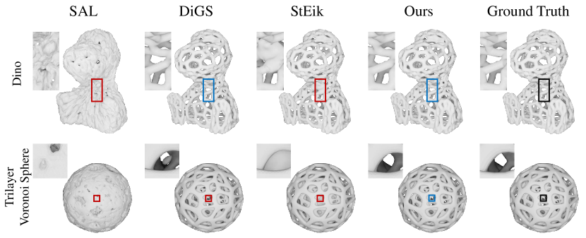
Figure 7: Visual examples on high genus dataset. Our method uses significantly less iterations but successfully reconstructs the correct topology for all shapes, whereas generate extra boundaries.

Fig. 1 and Fig. 7 shows the reconstruction of high genus surfaces from Mehta et al. [1]. Existing methods struggle with the complex topology, while our method can accurately reconstruct both the surface and the signed distance function.

In the supplementary material, we further present evaluations on other high genus shapes from Mehta et al. and the SRB dataset.

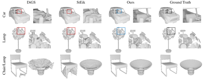
Figure 8: Visual results of DiGS [3], StEik [4], and HotSpot on ShapeNet [47]. Previous methods generate extra boundaries and fail to escape local optima, while our method successfully reconstructs the correct topology.

	IoU $\uparrow$	$d_{C}$ $\downarrow$	$d_{H}$ $\downarrow$	RMSE $\downarrow$	MAE $\downarrow$	SMAPE $\downarrow$	RMSE0.1	MAE0.1	SMAPE0.1
SAL [49]	0.7400	0.0074	0.0851	0.0251	0.0142	0.1344	0.0245	0.0182	0.6848
SIREN wo/ n [31]	0.4874	0.0051	0.0558	0.5009	0.4261	1.2694	0.0513	0.0382	0.8858
DiGS [3]	0.9636	0.0031	0.0435	0.1194	0.0725	0.2140	0.0152	0.0081	0.1760
StEik [4]	0.9641	0.0032	0.0368	0.0387	0.0248	0.0931	0.0147	0.0081	0.1770
Ours	0.9796	0.0029	0.0250	0.0281	0.0176	0.0540	0.0094	0.0047	0.1206

Table 3: Surface reconstruction metrics on ShapeNet [47], where $d_{C}$ and $d_{H}$ stand for the Chamfer and Hausdorff distances, RMSE, MAE, and SMAPE are distance field metrics, and RMSE_0.1, MAE_0.1, and SMAPE_0.1 are the same distance field metrics but only for points within distance $0.1$ of the surface. See the supplementary material for detailed results.

5.4 Sphere Tracing

Fig. 9 shows a visualization of number of steps a sphere tracer [21] takes to render the shapes obtained by SAL, DiGS, StEik, and our method. Our method leads to the least amount of iterations on average, since it generates smooth and accurate signed distance functions, which are crucial for rendering high-quality surfaces. More results can be found in the supplementary material.

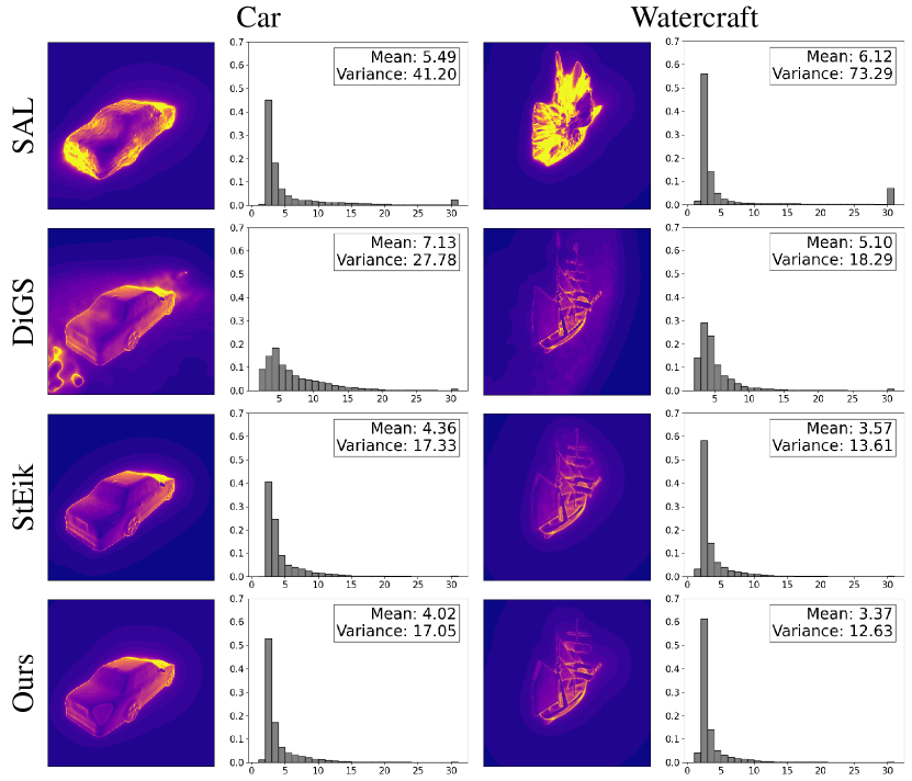
Figure 9: Visualizations and statistics of sphere tracing [21] iteration counts required to locate the surface. In the visual results brighter pixels indicating higher iteration counts. The histograms show the distribution of iterations for all pixels across 10 different camera poses. HotSpot finds the surface in fewer steps.

6 Discussion

Determining absorption coefficient $\lambda$. The absorption coefficient $\lambda$ has the units of $[\text{L}]^{-1}$, where L denotes a length unit. Rescaling the space is equivalent to rescaling $\lambda$ in the equation. While a larger $\lambda$ can improve accuracy, it introduces two challenges. First, our heat loss includes the factor $e^{-2\lambda|u|}$, which may become smaller than the precision limit of floating-point numbers, leading to round-off errors. Second, even if round-off errors are ignored, a large $\lambda|u|$ may reduce the optimizer’s ability to accurately shape the field. However, even with this, our loss will still push $u$ away from $0$, preventing the introduction of extra surfaces where $\lambda|u|$ should be large. We compensate by adding the eikonal loss together with our heat loss. When $\lambda|u|$ is large, the eikonal loss becomes the dominant term. Our scheduler for $\lambda$ also effectively shapes the distant regions. Spatially-adaptive parameters can potentially further improve the results.

Necessity of firm boundary condition. The heat diffusion of the screened Poisson equation is based on a well established boundary condition, and we enforce the boundary condition through the boundary loss over a discrete set of points, and rely on the spectral bias of neural networks [51] to interpolate them. When the input point set is sparse and the absorption coefficient $\lambda$ is high, an overly strong heat loss ($w_{b}$ being too small) can tear the boundary, causing the signed distance function to degrade into an unsigned distance one like Fig. 5. Thus, our theory suggests that a key insight is to set a high boundary weight $w_{b}$, while adjusting the absorption coefficient $\lambda$ to match the input point cloud density or by scaling the point cloud itself. Our experiments show that with proper parameter setting and rescaling the collapse can be avoided. Future research is required for very sparse boundary, and application to inverse rendering.

7 Conclusion

We propose a new model for neural signed distance function optimization based on screened Poisson equation. We analyze our loss theoretically and show that it can converge to the true distance, is stable both to a small perturbation and in the temporal dynamics, and penalizes large surface area. Our experiments show that our method reconstructs both better surfaces and better distance approximations compared to many existing methods, especially on complex and high-genus shapes.

Supplementary Material

Appendix A Proofs and Derivations

A.1 Proposition 1 proof.

Here we analyze the 2D case, but the following derivation naturally generalizes to 3D. We denote $\frac{\partial u}{\partial x}$ as $p_{1}$, $\frac{\partial u}{\partial y}$ as $p_{2}$, and let $n^{2}(x,y)=p_{1}^{2}+p_{2}^{2}$. Following the derivation from Kulyabov et al. [52], we can obtain the characteristics equations as follows. For any $a\neq 0$ if any field $u$ satisfies the eikonal equation,

$$\begin{split}\frac{p_{1}}{a}\frac{\partial p_{1}}{\partial x}+\frac{p_{2}}{a}\frac{\partial p_{1}}{\partial y}=\frac{n}{a}\frac{\partial n}{\partial x}\\ \frac{p_{1}}{a}\frac{\partial p_{2}}{\partial x}+\frac{p_{2}}{a}\frac{\partial p_{2}}{\partial y}=\frac{n}{a}\frac{\partial n}{\partial y}\end{split}$$ (18)

This implies that any curve $(x(s),y(s))$ satisfying $\frac{dx}{ds}=\frac{p_{1}}{a},\frac{dy}{ds}=\frac{p_{2}}{a}$ is the characteristic curve of $p_{1}$ and $p_{2}$. Let $a=n^{2}$,

$$\begin{split}\frac{du}{ds}&=u_{x}\frac{dx}{ds}+u_{y}\frac{dy}{ds}=p_{1}\frac{dx}{ds}+p_{2}\frac{dy}{ds}\\ &=\frac{p_{1}^{2}+p_{2}^{2}}{a}\equiv 1\end{split}$$ (19)

This equation holds for both $u$ and $u^{\prime}$ when we take the characteristic curve as

$$\left\{\begin{aligned} \frac{dx}{ds}&=\frac{u_{x}}{u_{x}^{2}+u_{y}^{2}},\\ \frac{dy}{ds}&=\frac{u_{y}}{u_{x}^{2}+u_{y}^{2}}\end{aligned}\right.$$ (20)

We assume $s\in(0,M)$ ($M>0$ can be infinity) is a differentiable domain which makes every derivative exist and all of these equations hold. Then we prove such a parametric curve is a ray or a segment.

$$\begin{split}\frac{d}{ds}u_{x}&=u_{xx}\frac{dx}{ds}+u_{xy}\frac{dy}{ds}=u_{xx}\frac{u_{x}}{n}+u_{xy}\frac{u_{y}}{n}\\ &=\frac{1}{2n}(2u_{x}u_{xx}+2u_{y}u_{xy})\\ &=\frac{1}{2n}\frac{\partial(u_{x}^{2}+u_{y}^{2})}{\partial x}\equiv 0\end{split}$$ (21)

Similarly, $u_{y}$ is also a constant. Then the direction vector in Eq. 20 is also a constant vector. Hence, $(x(s),y(s))$ is a ray or a segment. Given $u(x_{0},y_{0})=u_{0}$, we can solve this ordinary differential equation and obtain $u(x(s),y(s))=u_{0}+s$. Respectively, $u^{\prime}(x_{0},y_{0})=u_{0}+u_{0e}$ and $u^{\prime}(x(s),y(s))=u_{0}+s+u_{0e}$. On this parametic line, we have the following.

$$u^{\prime}(\bm{x}(s))-u(\bm{x}(s))=u_{0e}.$$ (22)

A.2 Proposition 2 proof.

We first consider the 3D case. First, for the original solution of Eq. 4, we denote it as $h$. For the following disturbance equation, we denote its solution as $h_{e}$:

$$\left\{\begin{aligned} &(\nabla^{2}-\lambda^{2})h_{e}=0\quad\forall\bm{x}\in\mathbb{R}^{3}\setminus B(\bm{x_{0}},\epsilon)\\ &\lim_{||\bm{x}||\to\infty}h_{e}<\infty,\;h_{e}(\bm{x})=h_{0e}\;\forall\bm{x}\in\partial B(\bm{x_{0}},\epsilon)\end{aligned}\right.$$ (23)

Then the disturbed $h^{\prime}=h_{e}+h$ still satisfies the screened Poisson equation in $\mathbb{R}^{d}\setminus(B\cup\Gamma)$. Given the spherical condition, we can analytically solve this equation by transforming it to an ordinary differential equation. Knowing that $\nabla^{2}h(r)=r^{-2}\cdot d(r^{2}\frac{dh}{dr})/dr$, we have:

$$\begin{split}&\Leftrightarrow\frac{1}{r^{2}}\frac{d}{dh}\left(r^{2}\frac{dh}{dr}\right)-\lambda^{2}h=0\\ &\Leftrightarrow\frac{1}{r^{2}}\left(2r\frac{dh}{dr}+r^{2}\frac{d^{2}h}{dr^{2}}\right)-\lambda^{2}h=0\\ &\Leftrightarrow\frac{d^{2}h}{dr^{2}}+\frac{2}{r}\frac{dh}{dr}-\lambda^{2}h=0\\ &\Leftrightarrow h(r)=\frac{Ae^{-\lambda r}}{r}+\frac{Be^{\lambda r}}{r},\quad r\geqslant\epsilon\end{split}$$ (24)

Given the boundary conditions, we obtain $A=\epsilon h_{0e}e^{\lambda\epsilon}$ and $B=0$. Consequently, the solution is as follows.

$$h_{e}(r)=\frac{\epsilon}{r}h_{0e}e^{\lambda(\epsilon-r)},\quad\forall r\geqslant\epsilon$$ (25)

We can further extend our analysis to 2D. Given $\nabla^{2}h(r)=r^{-1}\cdot d(r\frac{dh}{dr})/dr$, we have another ODE in 2D:

$$\begin{split}&\Leftrightarrow\frac{d^{2}h}{dr^{2}}+\frac{1}{r}\frac{dh}{dr}-\lambda^{2}h=0\\ &\Leftrightarrow r^{2}\frac{d^{2}h}{dr^{2}}+r\frac{dh}{dr}-\lambda^{2}r^{2}h=0\\ &\Leftrightarrow z^{2}\frac{d^{2}h}{dz^{2}}+z\frac{dh}{dz}-z^{2}h=0,\quad z=\lambda r\end{split}$$ (26)

Then we find it becomes a modified Bessel function with the following general solution:

$$h(z)=AK_{0}(z)+BI_{0}(z),$$ (27)

where $K_{0}$ represents the modified Bessel function of the second kind and $I_{0}$ represents the modified Bessel function of the first kind. Given the boundary conditions, we obtain $A=\frac{h_{0e}}{K_{0}(\lambda\epsilon)}$ and $B=0$. Then we place $r$ back and have the final solution as follows:

$$h(r)=\frac{e^{-\lambda\epsilon}}{K_{0}(\lambda\epsilon)}K_{0}(\lambda r)$$ (28)

It should be noted that $K_{0}$ converges to $0$ when $\lambda r$ goes infinity. More precisely, $K_{0}(\lambda r)$ and $e^{-\lambda r}/\sqrt{\lambda r}$ are infinitesimals of the same order [53]. Related property then becomes similar to 3D case.

A.3 Convergence speed proof.

Here we consider the 3D case. For single point $\bm{x}$, given the following screened Poisson equation

$$\left\{\begin{aligned} &(\nabla^{2}-\lambda^{2})h=0\quad\forall\bm{x}\in\mathbb{R}^{3}\setminus B(\bm{x_{0}},\epsilon)\\ &\lim_{||\bm{x}||\to\infty}h=0,\;h(\bm{x})=e^{-\lambda\epsilon}\;\forall\bm{x}\in\partial B(\bm{x_{0}},\epsilon)\end{aligned}\right.$$ (29)

Its solution is similar to Eq. 25:

$$h(r)=\frac{\epsilon}{r}e^{-\lambda r},\quad\forall r\geqslant\epsilon$$ (30)

Then we denote $S_{i}=\partial B(\bm{x}_{i},\epsilon)$, $h_{i}$ is the corresponding single point solution, $r_{0}$ is the minimum distance for any two points from $\Gamma$. When $\epsilon<r_{0}$ and $\lambda$ is large enough, we can assume that when $i\neq j$, $h_{j}(S_{i})=h_{j}(\bm{x}_{i})$. Given a finite set of boundary points $\Gamma=\{\bm{x}_{1},\bm{x}_{2},\dots,\bm{x}_{N}\}$ that is the input of the signed distance function reconstruction task, we can use a linear combination of single point solutions to obtain a new function satisfying the screened Poisson equation and a new boundary condition that is:

$$\left\{\begin{aligned} &(\nabla^{2}-\lambda^{2})h=0\quad\forall\bm{x}\in\mathbb{R}^{3}\setminus\cup_{\forall i}B(\bm{x_{i}},\epsilon)\\ &\lim_{||\bm{x}||\to\infty}h=0,\quad h(\bm{x})=e^{-\lambda\epsilon}\quad\forall\bm{x}\in\cup_{\forall i}S_{i}\end{aligned}\right.$$ (31)

We then set the boundary condition equation to solve the coefficients:

$$\begin{pmatrix}h_{1}(S_{1})&h_{2}(S_{1})&\cdots&h_{N}(S_{1})\\ h_{1}(S_{2})&h_{2}(S_{2})&\cdots&h_{N}(S_{2})\\ \vdots&\vdots&\ddots&\vdots\\ h_{1}(S_{N})&h_{2}(S_{N})&\cdots&h_{N}(S_{N})\end{pmatrix}\begin{pmatrix}c_{1}\\ c_{2}\\ \vdots\\ c_{N}\end{pmatrix}=\begin{pmatrix}e^{-\lambda\epsilon}\\ e^{-\lambda\epsilon}\\ \vdots\\ e^{-\lambda\epsilon}\end{pmatrix}$$ (32)

We denote the matrix here as $H\in\mathbb{R}^{N\times N}$. Its every diagonal element is $e^{-\lambda\epsilon}$, which is the largest in that row. This equation has at least one solution $C\in\mathbb{R}^{N}$ and every $c_{i}\in(0,1)$. Finally, $h=(h_{1},\dots,h_{N})C$ is the solution of Eq. 31. If we set $r_{i}={||\bm{x}-\bm{x}_{i}||}_{2}$, then

$$h(\bm{x})=\epsilon\sum_{i=1}^{n}c_{i}\frac{e^{-\lambda r_{i}}}{r_{i}}$$ (33)

Now we analyze the bound of $\frac{1}{\lambda}\ln(h_{\lambda}(\bm{x}))+d_{\Gamma}(\bm{x})$. First, we prove its upper bound is $\frac{1}{\lambda}[\ln\frac{\epsilon}{d_{\Gamma}(\bm{x})}+\ln(N)]$.

$$\frac{1}{\lambda}\ln h +d_{\Gamma}=\frac{1}{\lambda}\left(\ln\epsilon+\ln\sum_{i=1}^{n}c_{i}\frac{e^{-\lambda r_{i}}}{r_{i}}\right)+d_{\Gamma}$$ (34)

$$\leqslant\frac{1}{\lambda}\left(\ln\epsilon+\ln\frac{e^{-\lambda d_{\Gamma}}}{d_{\Gamma}}+\ln\sum_{i=1}^{N}c_{i}\right)+d_{\Gamma}$$

$$\leqslant\frac{1}{\lambda}\left(\ln\frac{\epsilon}{d_{\Gamma}}+\ln N\right)$$

Here, the first inequality holds because $d_{\Gamma}\leqslant r_{i}$ for all $i$ and every $h_{i}(r)$ is monotonically decreasing w.r.t. $r$. Then every $c_{i}<1$, so we can obtain the second inequality.

Second, we prove its lower bound is $\frac{1}{\lambda}\ln\frac{\epsilon}{d_{\Gamma}(\bm{x})}$.

For any row in Eq. 32, since we know that the largest element is on the diagonal equal to $e^{-\lambda\epsilon}$, we have

$$e^{-\lambda\epsilon}=\sum_{i=1}^{N}c_{i}h_{i}(S_{j})\leqslant\sum_{i=1}^{N}c_{i}h_{j}(S_{j})=e^{-\lambda\epsilon}\sum_{i=1}^{N}c_{i}$$ (35)

Hence, $\sum_{i=1}^{N}c_{i}\geqslant 1$. Next, we can set $h_{0}(r_{i})=h_{i}(\bm{x})$, where $h_{0}$ is the decay pattern in Eq. 30. $h_{0}$ is a convex and monotonically decreasing function so that we can apply these inequalities.

$$\begin{split}\frac{1}{\sum_{i=1}^{N}c_{i}}h(\bm{x})=\frac{\sum_{i=1}^{N}c_{i}h_{0}(r_{i})}{\sum_{i=1}^{N}c_{i}}\\ \geqslant h_{0}(\frac{\sum_{i=1}^{N}c_{i}r_{i}}{\sum_{i=1}^{N}c_{i}})\geqslant h_{0}(d_{\Gamma}(\bm{x}))\end{split}$$ (36)

Given $\sum_{i=1}^{N}c_{i}\geqslant 1$, we have $h(\bm{x})\geqslant\epsilon\frac{e^{-\lambda d_{\Gamma}}}{d_{\Gamma}}$. By basic transformations of this, we obtain the whole inequality as follows:

$$\frac{1}{\lambda}\ln\frac{\epsilon}{d_{\Gamma}}\leqslant d_{\Gamma}-|u_{\lambda}|\leqslant\frac{1}{\lambda}\left(\ln\frac{\epsilon}{d_{\Gamma}}+\ln N\right)$$ (37)

where $|u_{\lambda}|=-\frac{1}{\lambda}\ln h_{\lambda}$. It should also be noted that $\ln\frac{\epsilon}{d_{\Gamma}(\bm{x})}$ is a constant scalar field so that when $\bm{x}$ is fixed and $\lambda$ increases to infinity, $d_{\Gamma}-|u_{\lambda}|$ is first-order infinitesimal.

Appendix B Experiments

In all of our experiments, we use $p=1$ for Eq. 2 and Eq. 3.

B.1 2D Dataset

Fig. 10 provides an overview of the ground truths in the 2D dataset. Starting with simple shapes from DiGS [3] and StEik [4], we extended the dataset to include 14 shapes. We generate a total of 150,000 points along the boundaries in a single vector image. For each iteration, we randomly select 10% of the generated points to compute the boundary loss.

In our first 2D experiments (Table 5), we adopt the original hyperparameters and settings from DiGS [3] and StEik [4] as our baselines, making only one modification: extending the training iterations from 10k to 20k to better learn complex shapes.

In our setup, we compute the heat loss using the importance sampling method, which combines a mixture distribution of 1:1 uniform samples in $[-1.5,1.5]^{2}$ and Gaussian samples with an isotropic $\sigma=0.5$. For each iteration, we use 4,096 points for both the uniform and Gaussian samples, whereas DiGS and StEik generate 15,000 points to compute their derivative-based loss. We fix $\lambda$ in the heat loss while employing two schedulers: one for the heat loss and another for the eikonal loss. Towards the end of training, the heat loss is gradually weakened, and the eikonal loss is strengthened. This strategy aligns with the approach used in DiGS and StEik. Our results are presented in Fig. 10 as well. However, as shown in the ablation study (Table 2), removing the scheduler does not result in significant differences.

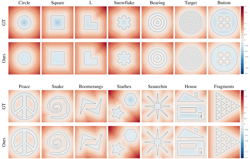
Figure 10: This figure illustrates all the 14 vector shapes in our 2D dataset. Each visualization is within the range ${[-1.2,1.2]}^{2}$. Spanning a spectrum from simple to complex, the dataset encompasses various topologies, smooth and irregular boundaries, as well as configurations with single and multiple objects. Our HotSpot model accurately reconstructs all the curves while preserving their correct topologies.

We also visualize the outcomes of the baseline methods in Fig. 11. In the ablation study, the boundary loss coefficient remains constant and identical across all experiments, and the same scheduler is applied to the eikonal loss. We also adopted the original loss weight ratios from the experiments of DiGS [3] in the fourth column and StEik [4] in the seventh column. All losses, except for the eikonal loss, are applied without a scheduler. The outputs of the original DiGS and StEik models are also shown in the fifth and eighth columns, respectively.

All other models make some errors in topology. Even when their topologies are correct, details like the Target and House shapes in the first two columns are missing. When using a relatively smaller learning rate in the ablation study for DiGS and StEik, the outputs become overly flat, despite maintaining the same ratio among the loss weights from their paper. This can be interpreted as a limitation of their derivative-based losses, which, as a corollary of the eikonal equation, only serve as a necessary condition for the equation, encouraging the condition $|\nabla u|=c$, where $c$ can be any constant. With a small learning rate, their losses trap the outputs to $|\nabla u|=0$.

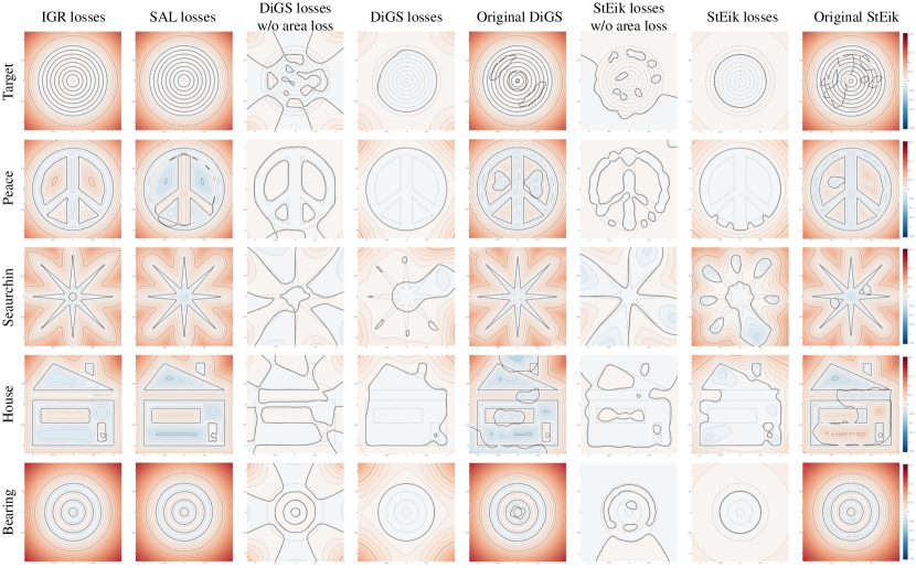
Figure 11: This figure demonstrates how the baselines fail with complex shapes. The difference between the fourth and fifth columns (from left to right), as well as between the seventh and eighth columns, is that the former one is generated in the ablation study, while the other is generated by the original model. Dashed lines represent the true boundaries, while the boldest line indicates the reconstructed boundaries.

In our framework, we analyze the influence of different values of $\lambda$ and various coefficients of the eikonal loss, with visualizations presented in Fig. 12. This experiment replicates the settings from the ablation study, except for the values of $\lambda$, $w_{e}$, and the iteration number, with all schedulers removed. To ensure full convergence, we extend the training iterations from 20k to 200k.

From Fig. 3 and Fig. 12, we observe the influence from different $\lambda$. When $\lambda$ is very small, heat from the boundaries diffuses to distant regions, causing $h\approx 1$ almost everywhere in the test region. As a result, $u\approx 0$ across the domain, leading to an overly flat signed distance function with many extra boundaries. As $\lambda$ increases, the outputs become more regular. Notably, even without the eikonal loss, setting $\lambda=10$ yields outputs that are more regular than several baselines in Fig. 11. However, as $\lambda$ continues to increase, the factor $e^{-\lambda|u|}$ in the loss computation diminishes rapidly, especially where $|u|$ is large initially or grows during training. This makes optimization without the eikonal loss increasingly challenging and less effective. For instance, in the $\lambda=50$ and $\lambda=100$ subfigures with $w_{e}=0$, the values in the upper-right region remain greater than $1.0$ even after 200k iterations. Although our neural network provides some output values in these regions, they are significantly larger than the ground truth.

Incorporating the eikonal loss stabilizes the training process and promotes a more regular field. When $\lambda$ is small, the approximation from Eq. 5 is weakly achieved, but the eikonal loss helps regulate the output and prevents it from becoming overly flat. When $\lambda$ is large, the eikonal loss dominates in regions where $\lambda|u|$ is substantial. However, if the eikonal loss is overly strong, extra boundaries and local optima may re-emerge.

This does not mean that users must carefully balance the hyperparameters $w_{e}$, $w_{h}$, and $\lambda$. We have found effective ways to choose them. In our subsequent experiments, the schedulers for $\lambda$ and $w_{e}$ ensure robust shaping capabilities across various shapes and distance ranges in the ShapeNet dataset [47]. Mimicking a real annealing process, we gradually increase $\lambda$ and $w_{e}$, allowing the heat loss to shape and stretch most regions first, helping the optimization escape local optima. As the heat field cools due to the increasing absorption coefficient $\lambda$, the eikonal loss maintains the stretching and assumes control in remote regions.

Figure 12: Signed distance function reconstructions of the vector image House with varying values of $\lambda$ and $w_{e}$.

	IoU $\uparrow$			Chamfer Distance $\downarrow$			Hausdorff Distance $\downarrow$
	mean	median	std	mean	median	std	mean	median	std
DiGS [3]	0.7882	0.9359	0.2803	0.0055	0.0037	0.0046	0.1267	0.1350	0.1088
StEik [4]	0.6620	0.7305	0.3224	0.0073	0.0051	0.0068	0.1425	0.1654	0.1146
Ours	0.9870	0.9888	0.0083	0.0014	0.0013	0.0003	0.0153	0.0150	0.0100

Table 4: Comparison of 2D dataset reconstruction results.

	RMSE $\downarrow$			MAE $\downarrow$			SMAPE $\downarrow$
	mean	median	std	mean	median	std	mean	median	std
DiGS [3]	0.0597	0.0504	0.0511	0.0315	0.0253	0.0351	0.3363	0.2355	0.3414
StEik [4]	0.0725	0.0335	0.0903	0.0419	0.0108	0.0574	0.4222	0.2223	0.4409
Ours	0.0199	0.0189	0.0130	0.0101	0.0072	0.0060	0.0699	0.0693	0.0226

Table 5: Comparison of 2D dataset distance queries.

B.2 ShapeNet

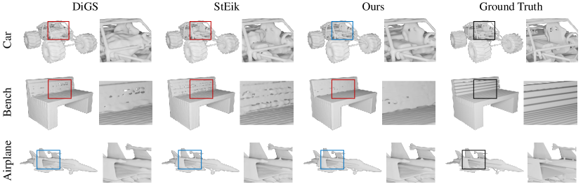
Figure 13: Additional results from the ShapeNet dataset. We present the bench, where none of the methods achieve a satisfactory surface reconstruction, and the airplane, where all methods successfully capture detailed structures.

We show full metrics for the ShapeNet dataset in Tables 6, 7, and 8. We compare our method with the state-of-the-art methods, including SAL [2], SIREN without normalization [31], DiGS [3], and StEik [4]. Our method outperforms all other methods in terms of surface reconstruction metrics, including IoU, Chamfer distance, and Hausdorff distance. In terms of distance query metrics, our method achieves the best performance in terms of RMSE, MAE, and SMAPE. In the near-surface region, our method also outperforms other methods in terms of RMSE, MAE, and SMAPE.

	IoU $\uparrow$			Chamfer Distance $\downarrow$			Hausdorff Distance $\downarrow$
	mean	median	std	mean	median	std	mean	median	std
SAL [2]	0.7400	0.7796	0.2231	0.0074	0.0065	0.0048	0.0851	0.0732	0.0590
SIREN wo/ n [31]	0.4874	0.4832	0.4030	0.0051	0.0038	0.0036	0.0558	0.0408	0.0511
DiGS [3]	0.9636	0.9831	0.0903	0.0031	0.0028	0.0016	0.0435	0.0168	0.0590
StEik [4]	0.9641	0.9848	0.1052	0.0032	0.0028	0.0028	0.0368	0.0172	0.0552
Ours	0.9796	0.9842	0.0203	0.0029	0.0028	0.0012	0.0250	0.0153	0.0360

Table 6: Surface reconstruction metrics on ShapeNet [47].

	RMSE $\downarrow$			MAE $\downarrow$			SMAPE $\downarrow$
	mean	median	std	mean	median	std	mean	median	std
SAL [2]	0.0251	0.0197	0.0270	0.0142	0.0116	0.0108	0.1344	0.1064	0.1032
SIREN wo/ n [31]	0.5009	0.4842	0.1769	0.4261	0.4027	0.1811	1.2694	0.9859	0.5195
DiGS [3]	0.1194	0.1107	0.0597	0.0725	0.0644	0.0423	0.2140	0.2162	0.0935
StEik [4]	0.0387	0.0338	0.0229	0.0248	0.0222	0.0142	0.0931	0.0843	0.0748
Ours	0.0281	0.0259	0.0136	0.0176	0.0160	0.0082	0.0540	0.0514	0.0243

Table 7: Overall distance query metrics on ShapeNet [47].

	RMSE near surface $\downarrow$			MAE near surface $\downarrow$			SMAPE near surface $\downarrow$
	mean	median	std	mean	median	std	mean	median	std
SAL [2]	0.0245	0.0252	0.0075	0.0182	0.0189	0.0059	0.6848	0.6890	0.2488
SIREN wo/ n [31]	0.0513	0.0401	0.0404	0.0382	0.0206	0.0351	0.8858	0.5406	0.7483
DiGS [3]	0.0152	0.0135	0.0081	0.0081	0.0074	0.0037	0.1760	0.1657	0.0660
StEik [4]	0.0147	0.0130	0.0070	0.0081	0.0074	0.0041	0.1770	0.1664	0.0859
Ours	0.0094	0.0078	0.0049	0.0047	0.0042	0.0020	0.1206	0.1163	0.0313

Table 8: Distance function query for near surface region on ShapeNet [47].

Our test region is defined in the same way as in DiGS and StEik. Both methods rescaled the circumscribed sphere centered at the geometric center of a point cloud to a unit sphere and designated the circumscribed cube $[-1,1]^{3}$ as their test region. We evaluate our results within the exact same coordinate system. During training, however, we rescale the point cloud to achieve an adaptive $\lambda$ described in the main text.

To compute the IoU and ground truth distances, we utilized the Occupancy Network [16] and a point cloud completion model [50]. A dense grid was generated within $[-1,1]^{3}$ to evaluate the metrics. For near-surface queries, we filtered points with a ground truth distance smaller than 0.1 to compute the accuracy, as presented in Table 8. Our method demonstrates a remarkable lead, reducing losses by more than one-third compared to the second-best model.

To illustrate the improved quality of our level sets, we also provide sectional views from different models for comparison in Fig. 14.

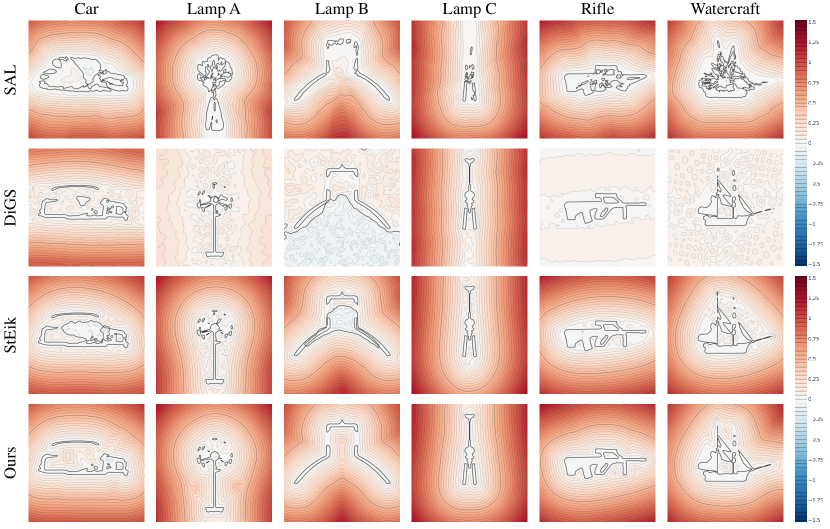
Figure 14: Sectional views of ShapeNet signed distance function reconstruction results. Car, Lamp A, and Lamp B are shown in Fig. 8, while Lamp C, Rifle, and Watercraft are presented in Fig. 9 and Fig. 18. By cross-verifying with them, our HotSpotachieves reconstructions with fewer extra boundaries, more regularized level sets, and accurate topologies.

Our level set near the surface is smoother and more regular, offering significant advantages for downstream tasks such as sphere tracing.

B.3 Complex Topology Reconstruction

Figure 15: Visualizations of Genus6, Kangaroo, and Voronoi Sphere from the Mehta et al [1]. dataset. We show the number of iterations used in training in the parenthesis. We achieve excellent results with only half the iterations, successfully capturing the correct topologies.

Figure 16: Visualizations of bilayer and trilayer Voronoi Spheres. Beyond achieving accurate topology reconstructions, the sectional views reveal that our level set is the only one free from chaotic and noisy interiors, ensuring meaningful representations.

We adopt five high-genus geometries from Mehta et al. [1] and generate 3D point clouds for them, including Bunny, Genus6, VSphere, Dino, and Kangaroo. Additionally, we use the mesh of VSphere to create bilayer and trilayer VSphere, resulting in a total of seven shapes with complex topologies. We compare our method with SAL [2], DiGS [3], and StEik [4] on these shapes, presenting the visual results in Fig. 1, Fig. 7, Fig. 15, and Fig. 16. Our method runs for 10k iterations. To ensure sufficient convergence and minimize extra boundaries, we run the other methods for 20k iterations on Bunny, Genus6, VSphere, Dino, and Kangaroo, and for 100k iterations on the bilayer and trilayer VSphere. Despite the increased iterations, the other methods fail to reconstruct the correct topology and generate extra boundaries, whereas our method successfully reconstructs the correct topology for all shapes.

B.4 Surface Reconstruction Benchmark (SRB)

SRB consists of 5 noisy scans, each containing point cloud and normal data. We compare our method against the current state-of-the-art methods on this benchmark without using the normal data. The results are presented in Table 9, where we report the Chamfer ($d_{C}$) and Hausdorff ($d_{H}$) distances between the reconstructed meshes and the ground truth meshes.

Additionally, we provide the corresponding one-sided distances ($d_{\vec{C}}$ and $d_{\vec{H}}$) between the reconstructed meshes and the input noisy point cloud. It is worth noting that one-sided distances are used here to maintain consistency with the historical choice of previous methods.

Our improvement is less pronounced compared to prior methods, as the SRB dataset represents a relatively simple benchmark without complex structures. Additional visual results are provided in Fig. 17.

Compare with	GT		Scans
Method	$d_{C}$	$d_{H}$	$d_{\vec{C}}$	$d_{\vec{H}}$
IGR wo n	1.38	16.33	0.25	2.96
SIREN wo n	0.42	7.67	0.08	1.42
SAL [2]	0.36	7.47	0.13	3.50
IGR+FF [44]	0.96	11.06	0.32	4.75
PHASE+FF [44]	0.22	4.96	0.07	1.56
DiGS [3]	0.19	3.52	0.08	1.47
StEik [4]	0.18	2.80	0.10	1.45
Ours	0.19	3.17	0.09	1.36

Table 9: Surface reconstruction metrics on SRB [48].

Figure 17: Visualization results on the SRB dataset. From left to right: Anchor, Daratech, DC, Garagoyle, and Lord Quas.

B.5 Sphere Tracing

For implementation details, we adopt the sphere tracing algorithm [21], as implemented in Yariv et al.’s work [36]. For each pixel, the algorithm advances along the ray by the signed distance function value at the current point, repeating this process until one of the following conditions is satisfied: convergence, where the SDF value falls below a threshold of $5.0\times 10^{-5}$; divergence, where the ray steps outside the unit sphere; or the maximum step limit of $30$ is reached.

For signed distance functions, we use trained models from SAL [2], DiGS [3], StEik [4], and our proposed method. The evaluation is conducted on five randomly selected objects (airplane, car, watercraft, rifle, and lamp) from ShapeNet [47]. For each object, we generate ten camera poses arranged in a circular trajectory around the central object, with a radius of $1.0$ and a height of $0.5$. The rendered images have a resolution of $500\times 500$ pixels.

Fig. 9 and Fig. 18 illustrate the number of steps required for each pixel until ray marching terminates under one of the three conditions described above. Brighter pixels correspond to rays that are harder to converge, requiring more queries, whereas our model produces relatively darker results compared to other models. Furthermore, the histograms for our model are more skewed to the left, highlighting its efficiency. These observations demonstrate that our model excels at early divergence detection in non-intersected regions and requires fewer steps to locate the surface in intersected regions. This efficiency stems from the smoothness and accuracy of our signed distance function, particularly its high quality near the surface, which significantly enhances the rendering performance of sphere tracing.

Because Fig. 9 and Fig. 18 only visualize the computation costs, to verify the accuracy of the object shapes in rendering, we visualize the depth and surface normals at the intersections. For rays that do not converge within 30 iterations, the intersection is approximated by identifying sign transitions at 100 equally spaced sampling points along the ray. The normal vector at the intersection, denoted by $\hat{x}$, is computed using Eq. 38 to enhance the visualization of the geometries. Non-intersected areas are masked in white. Fig. 19 demonstrates that our model accurately detects and represents the object’s surface in this downstream application, while other models show artifacts and distortions.

$$\hat{n}(\theta)=\frac{\nabla f(\hat{x}(\theta),\theta)}{\|\nabla f(\hat{x}(\theta),\theta)\|_{2}}.$$ (38)

These results demonstrate that in sphere tracing rendering, the distance query accuracy of our model effectively guides the ray toward the object’s surface, enhancing rendering efficiency. Additionally, its precision at the zero level set ensures an accurate representation of the object.

Figure 18: Visualization of iteration counts for each pixel and their corresponding histograms. The iteration count images are taken from two arbitrary poses, while the histograms gather outcomes across all ten rendered poses. Brighter pixels indicate a higher number of queries required for convergence before termination, while darker pixels signify fewer queries. The histograms clearly show that when rendering with our output, most pixels require fewer iterations to determine the surface.

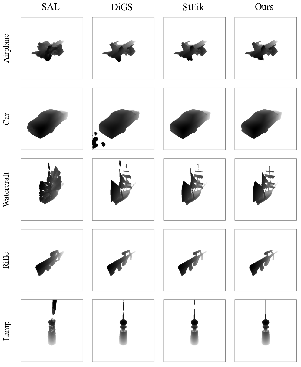
(a) Depth maps showcasing the distance from the camera to the surface.

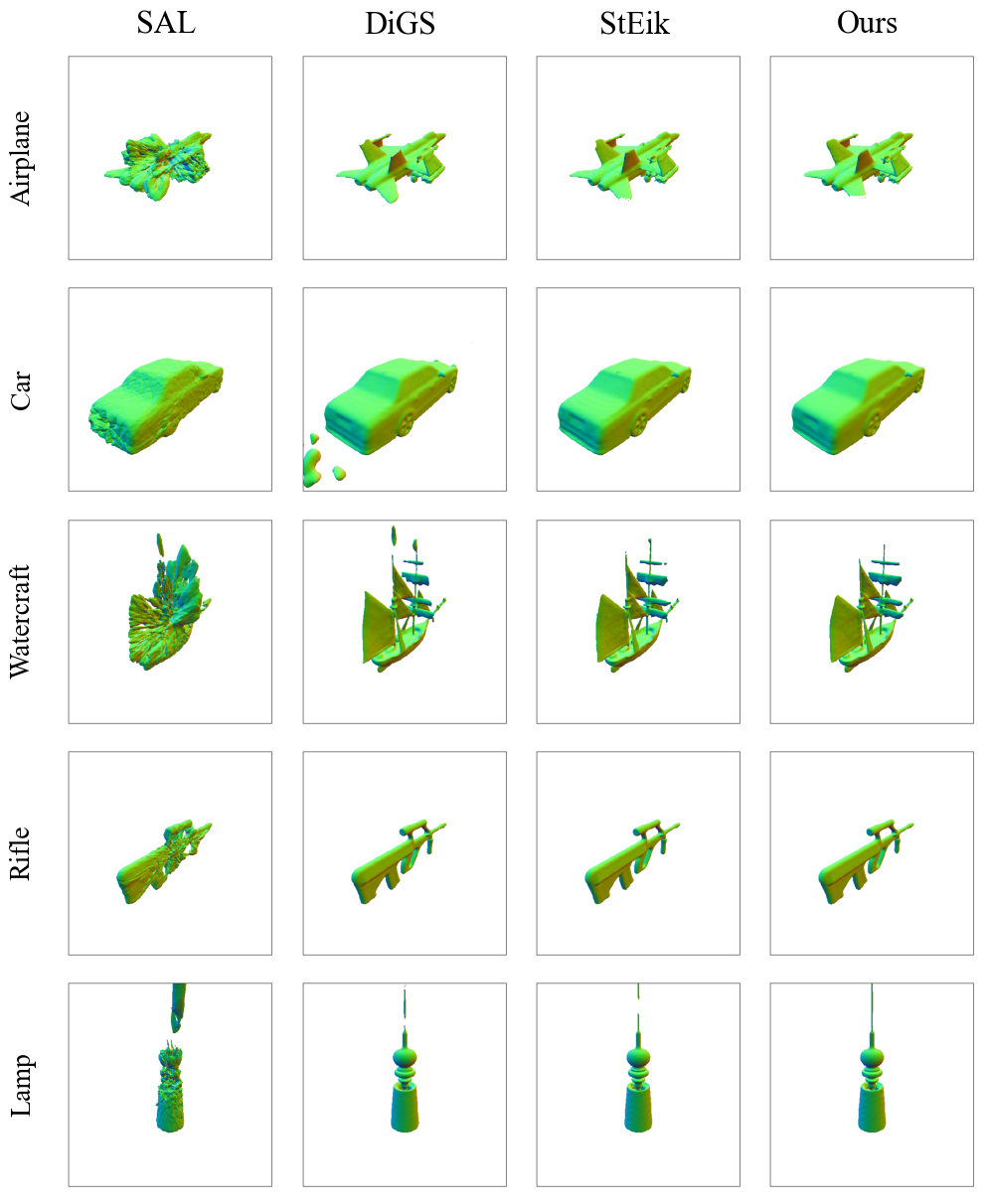
(b) Normal maps illustrating surface orientation at each point.

Figure 19: Rendering results with sphere tracing algorithm.

Appendix C Relation to PHASE [44]

While derived from very different mathematical principles and a different motivation, our method turns out to have a close relation to the PHASE model proposed by Lipman. The PHASE model essentially simulates two fluids finding equilibrium in a container by minimizing an energy functional. A smooth approximation of the indicator of different fluids is involved and interpreted as an occupancy function $o(\bm{x})$ such that $o$ outputs $1$ when outside of the object, $-1$ when inside the object, and $0$ when exactly on the surface. Lipman further adds a reconstruction loss to encourage $o(\bm{x})$ to vanish at the boundary and adapts the Van der Waals-Cahn-Hilliard theory of phase transitions [54, 55], resulting in the following functional to minimize:

$$\mathcal{F}(o)=w_{b}\mathcal{L}(o)+\int_{\Omega}\epsilon\|\nabla o\|^{2}+W(o),$$ (39)

where $w_{b}$ is the weight of the reconstruction loss, $\mathcal{L}(o)$ is the reconstruction loss that encourages $o$ to be zero at the boundary, $\epsilon$ is a small positive constant, and $W(o)$ is a potential. Lipman showed that by choosing a double-well potential $W(o)=o^{2}-2|o|+1$, the minimizer can be converted into an approximated signed distance function $s$ through a log transform:

$$s=-\sqrt{\epsilon}\ln\left(1-\left|o\right|\right)\text{sign}(o).$$ (40)

It turns out that our heat field $h$ when optimized under our heat loss is closely related to the regularized occupancy function $o$. If we set $h=1-|o|$ and $\lambda=\epsilon^{-\frac{1}{2}}$ and solve for the screened Poisson equation (Eq. 4), we would obtain PHASE’s regularized occupancy.

However, there are several crucial differences between our approach and PHASE where our theory and derivation has led to additional insights and huge differences in implementations and results.

First, based on a theoretical framework aiming the area minimization, PHASE’s theory promotes setting the weight $w_{b}$ of the boundary loss (Eq. 2) to $w_{b}=\epsilon^{\alpha}$ where $\alpha\in(\frac{1}{4},\frac{1}{2})$. However, we found that finding the exact minimal area is detrimental to the optimization, as discussed in Section 3. On the contrary, according to our theory and experiments, we find it necessary to maintain boundaries between points and set the weight $w_{b}$ to a much higher value to ensure the boundary condition of the screened Poisson equation is satisfied (Eq. 4), as states in main text.

Theorem 2 in the PHASE paper states that to achieve minimal area, $w_{b}$ should converge to $0$ as $\epsilon$ approaches an infinitesimal value. However, this interpretation does not align with the nature of the signed distance function reconstruction task which should complete the manifold and connect points, as discussed in Section 3, and may lead to unintended consequences as follows: When the boundary weight $w_{b}$ is overly small, the signed distance function values of boundary points cannot even converge to close to 0. When the weight $w_{b}$ is still not large enough, their output collapses from a surface-based-distance signed distance function to a point-cloud-based-distance unsigned distance function upon reaching the target where the boundaries are only point clouds and the area becomes almost zero. In contrast, our model demonstrates robust and accurate performance, effectively connecting points and interpolating boundaries by taking advantages of neural network’s spectral bias [51], with a large boundary weight $w_{b}$ and an adaptive absorption $\lambda$, as discussed in Section 6.

In addition to Fig. 5, we show more empirical results on our 2D dataset supporting our claim here in the supplementary. In Table 10, we show the visual results of PHASE on a single circle across different boundary weight choices, and compute the surface reconstruction and distance metrics. We show visual results on the rest of the 2D dataset in Fig. 21, and the mean metrics for each boundary loss weight over the whole 2D dataset in Table 11. In these experiments, we use eikonal loss weight $0.1$, as provided in the PHASE paper. We also show one example from ShapeNet in Fig. 20, where we use eikonal loss weight $1.0$. From our theory and the examples above, one can clearly see that using a small boundary loss weight is not the best strategy.

GT	$w_{b}=0.1$	$w_{b}=0.2$	$w_{b}=0.3$	$w_{b}=0.5$	$w_{b}=1.0$	$w_{b}=2.0$	$w_{b}=5.0$	$w_{b}=10.0$	$w_{b}=20.0$
IoU	0.3288	0.3330	0.3242	0.2975	0.2138	0.0022	0.9693	0.9912	0.9917
Chamfer	0.2244	0.2138	0.1955	0.1434	0.0777	0.0175	0.0080	0.0026	0.0025
Hausdorff	0.2315	0.2216	0.1991	0.1455	0.0799	0.1584	0.0150	0.0102	0.0105
RMSE	0.2318	0.2209	0.2085	0.1740	0.1477	0.1476	0.0481	0.0681	0.3004
MAE	0.2237	0.2122	0.1982	0.1552	0.1048	0.0556	0.0336	0.0610	0.2744
SMAPE	0.9159	0.8814	0.8404	0.7059	0.5333	0.3396	0.2028	0.3291	1.0863

Table 10: Comparison of PHASE results on a circle with different $w_{b}$ values. The color scale is the same as in Fig. 5.

$w_{b}$	$0.1$	$0.2$	$0.3$	$0.5$	$1.0$	$2.0$	$5.0$	$10.0$	$20.0$
IoU	0.2026	0.1843	0.2050	0.2089	0.2505	0.2061	0.3899	0.4838	0.4696
Chamfer	0.2663	0.3122	0.2504	0.1785	0.1067	0.0499	0.0793	0.0888	0.1030
Hausdorff	0.5692	0.7001	0.5635	0.4191	0.3446	0.3747	0.4567	0.4383	0.5407
RMSE	0.4644	0.3314	0.2382	0.1606	0.1111	0.0734	0.0567	0.0747	0.1282
MAE	0.4332	0.3114	0.2265	0.1500	0.0918	0.0413	0.0405	0.0623	0.1112
SMAPE	1.2558	1.1504	1.0870	0.9475	0.8107	0.5873	0.7191	0.8877	1.1477

Table 11: Mean metrics of PHASE results with different $w_{b}$ values on the full 2D dataset.

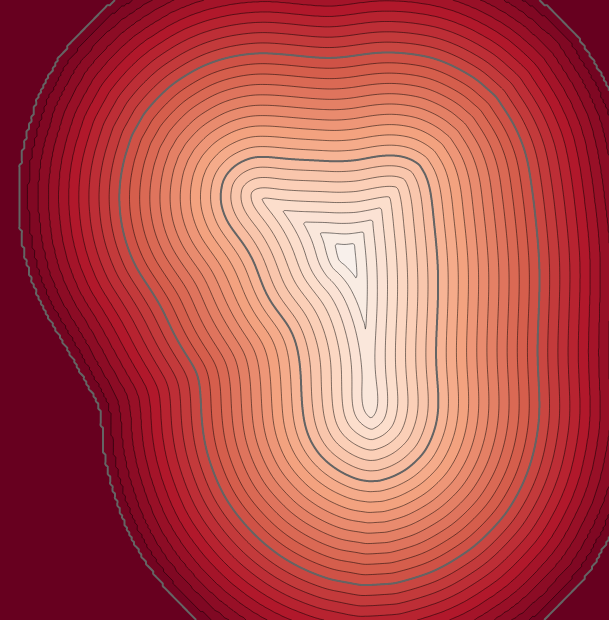
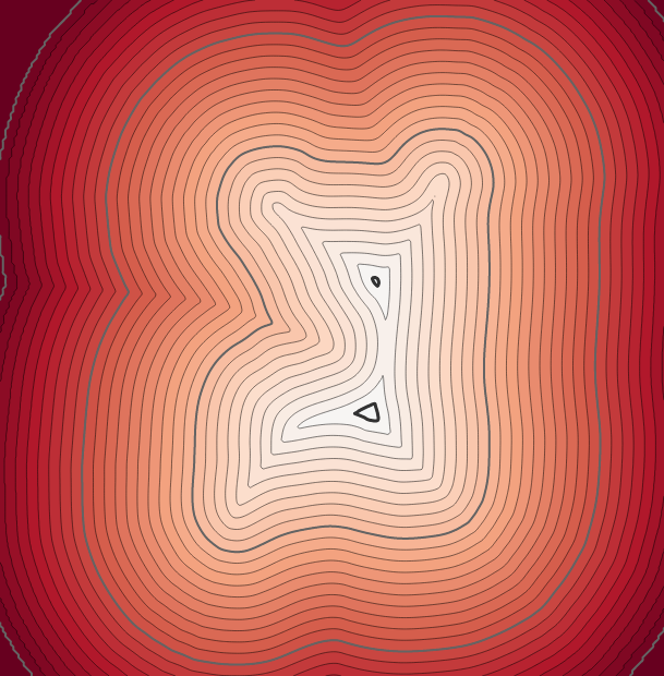
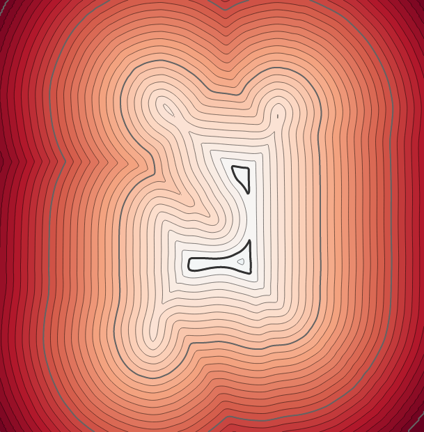
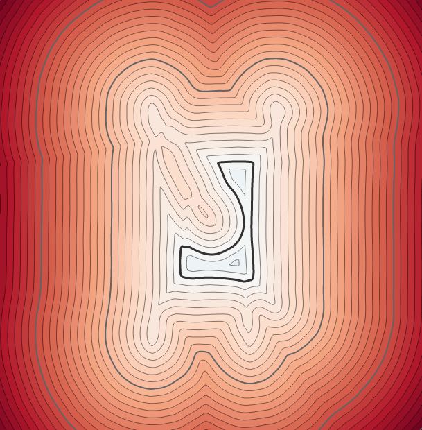
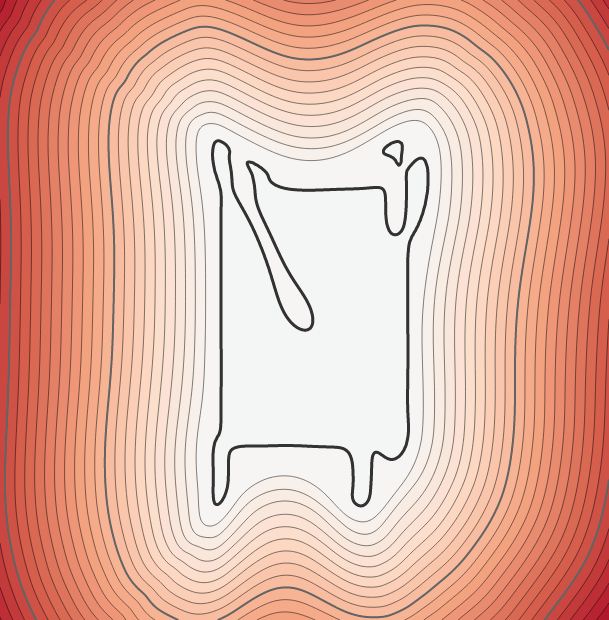
GT mesh	$w_{b}=0.1$	$w_{b}=0.2$	$w_{b}=0.3$	$w_{b}=0.5$	$w_{b}=1.0$	$w_{b}=5.0$	$w_{b}=10.0$	$w_{b}=20.0$
IoU	0.0000	0.0046	0.0387	0.1177	0.3106	0.9742	0.9638	0.9020
Chamfer	0.2056	0.2055	0.1749	0.1441	0.0935	0.0060	0.0065	0.0089
Hausdorff	0.4905	0.4909	0.4395	0.3855	0.3094	0.0518	0.0545	0.0651
RMSE	0.8656	0.8263	0.7944	0.7505	0.6588	0.4578	0.4275	0.4041
MAE	0.8468	0.8108	0.7769	0.7292	0.6339	0.4004	0.3528	0.3182
SMAPE	1.5123	1.5100	1.4956	1.4608	1.3912	1.1019	0.9778	1.0324

Figure 20: Comparison of PHASE results on a 3D cabinet with different $w_{b}$ values. SDF values are visualized only on a 2D plane. The color scale is the same as in Fig. 5.

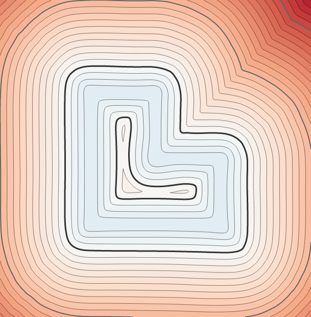
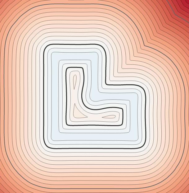
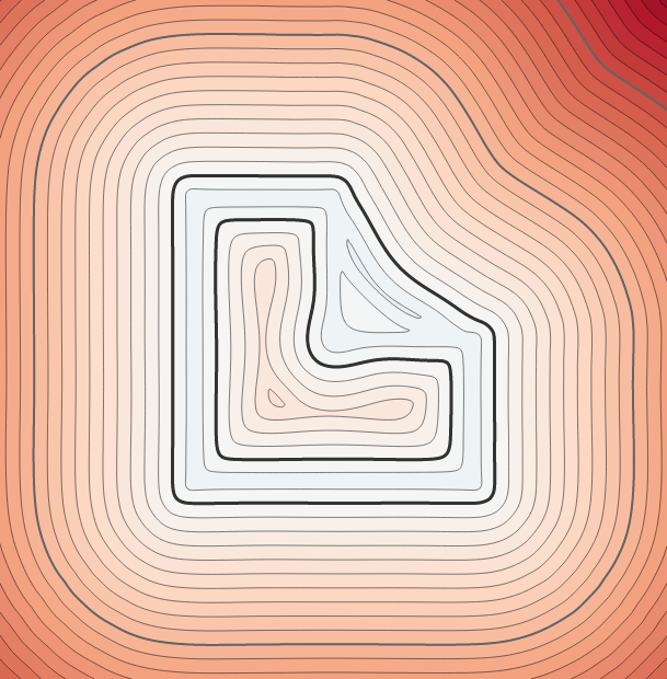
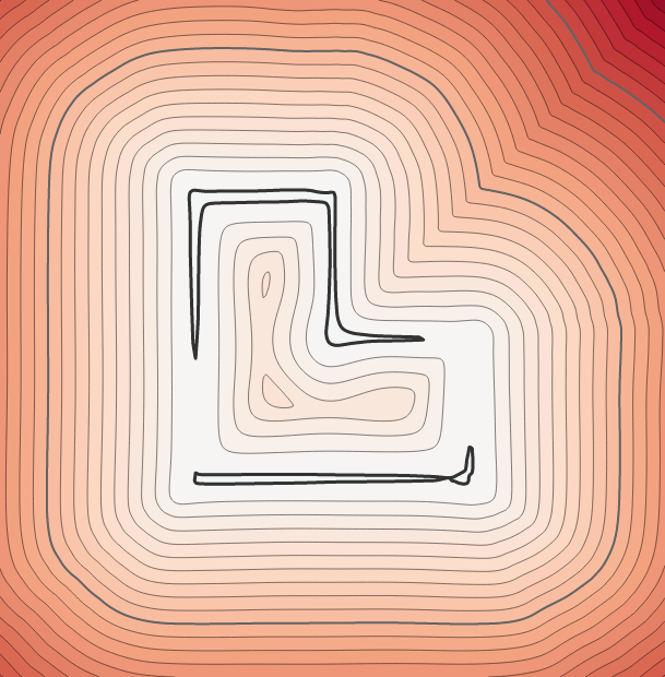
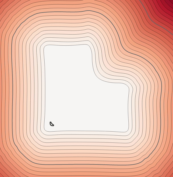
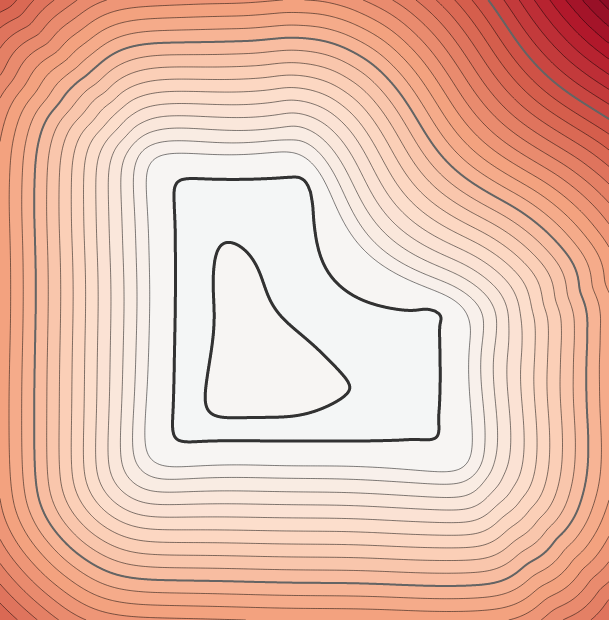
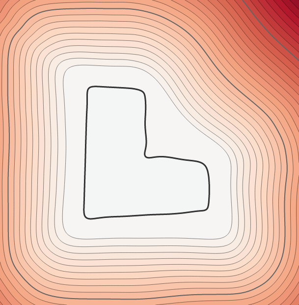
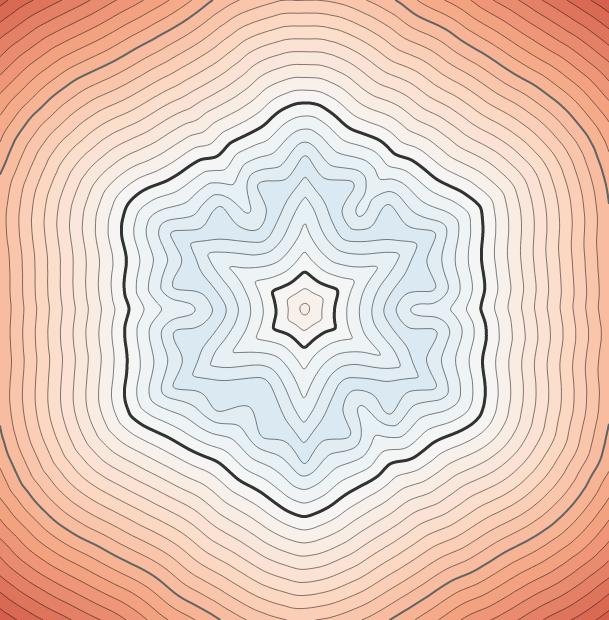
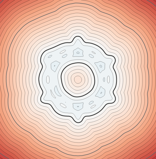
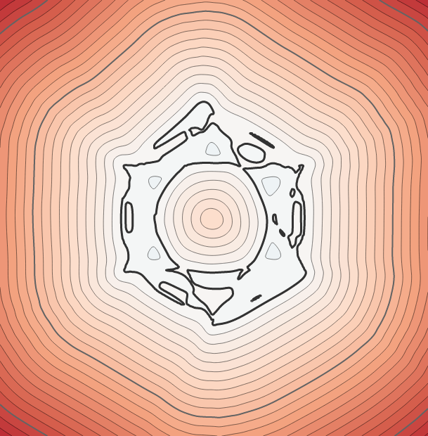
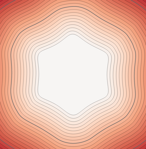
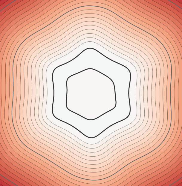
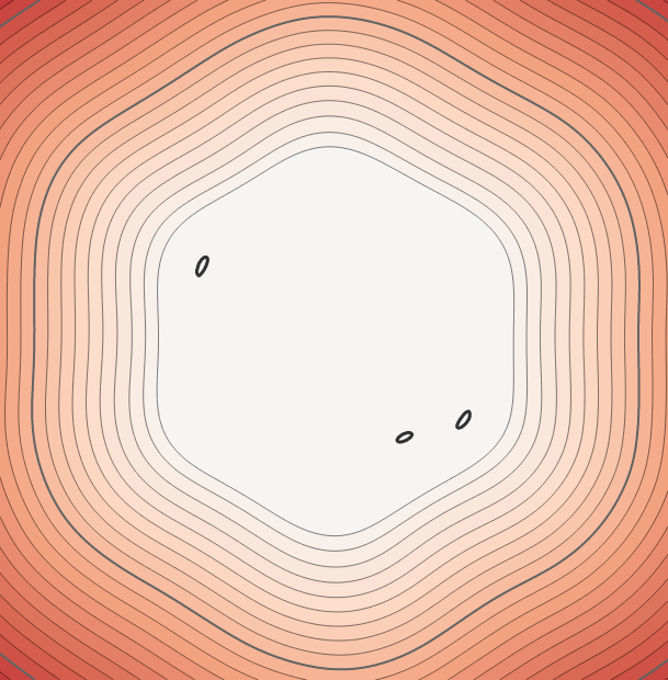
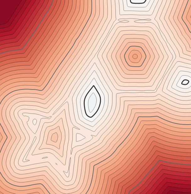
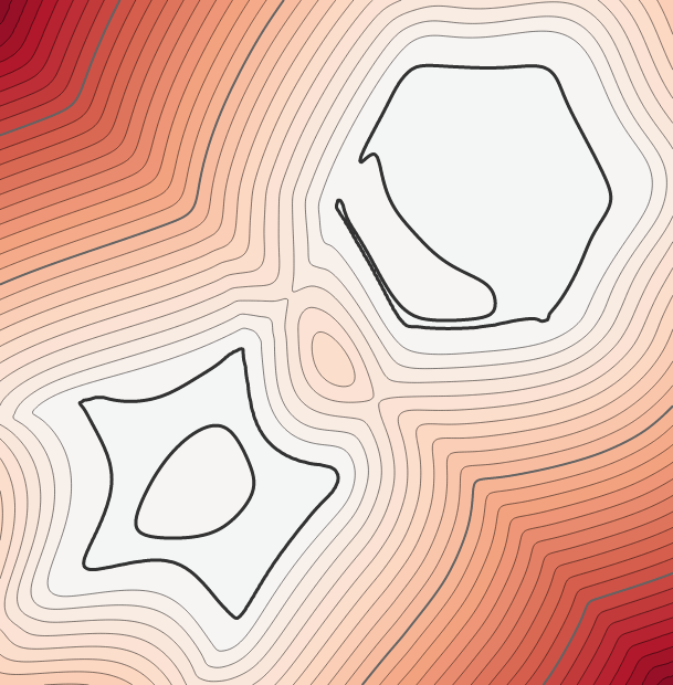
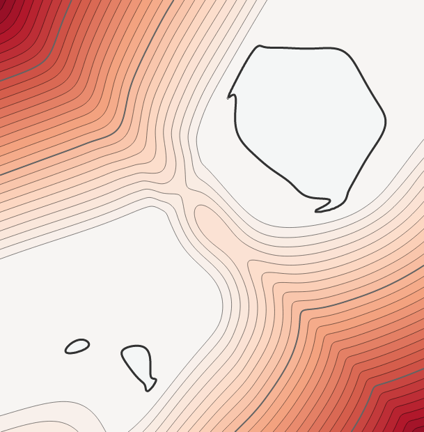
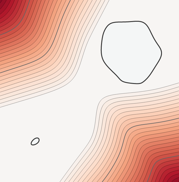
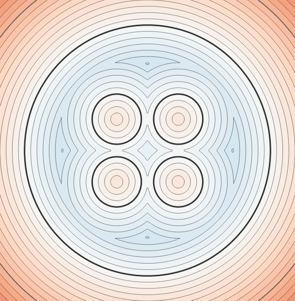
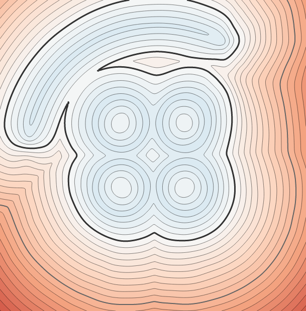
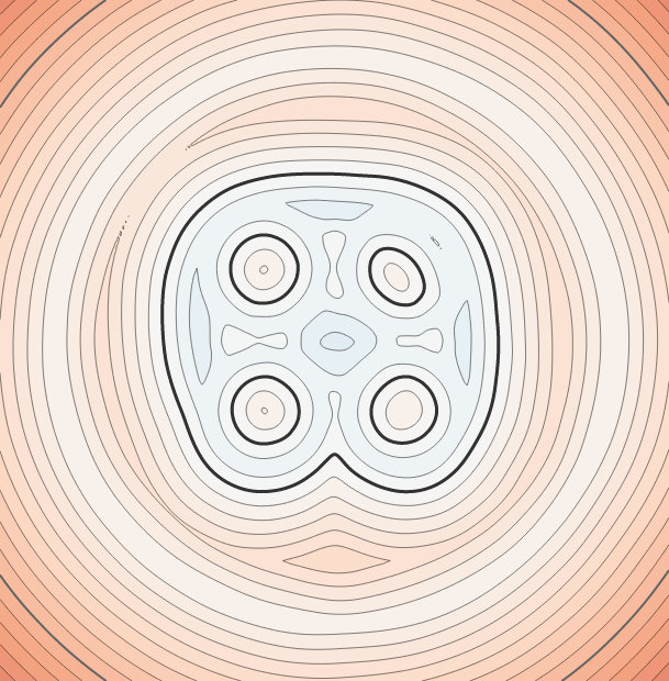
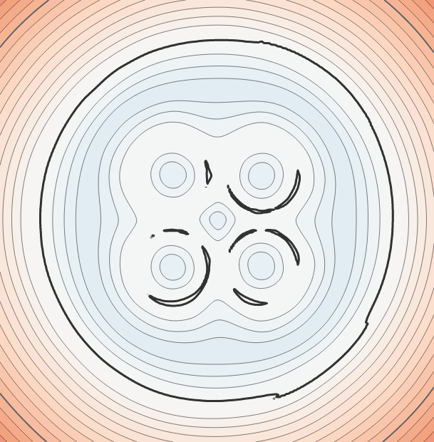
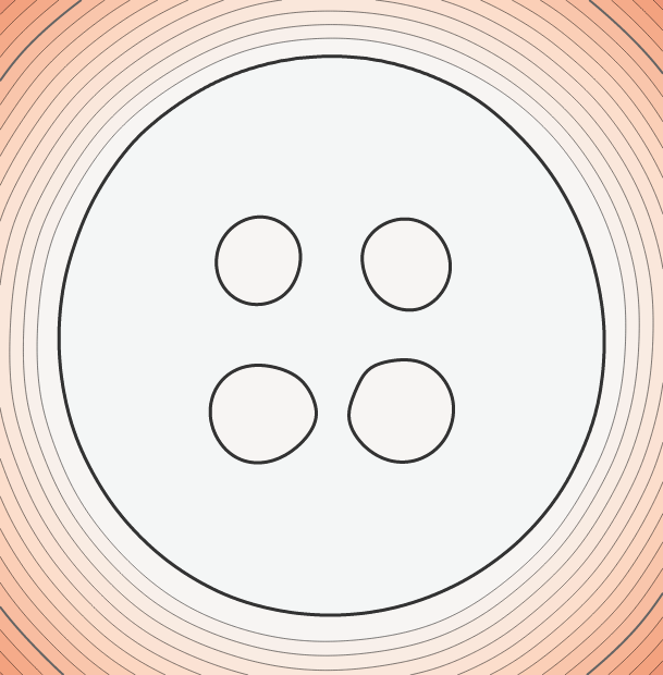
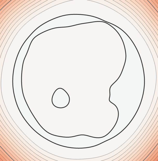
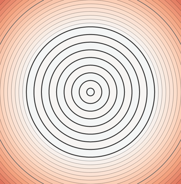
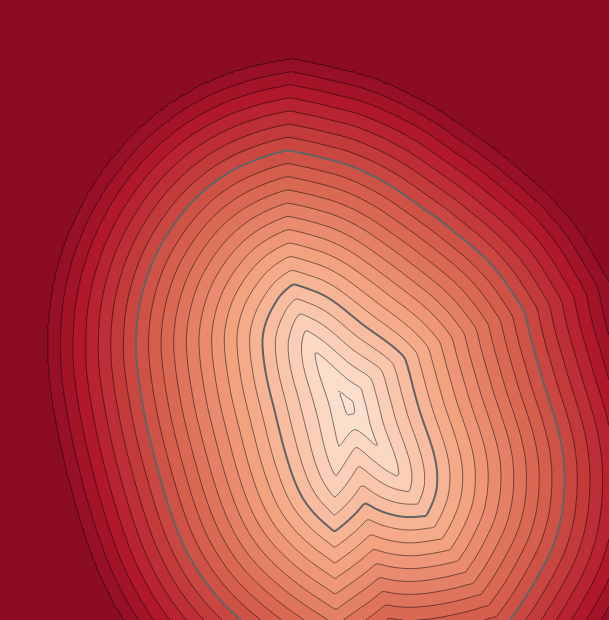
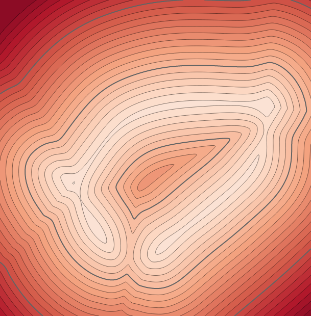
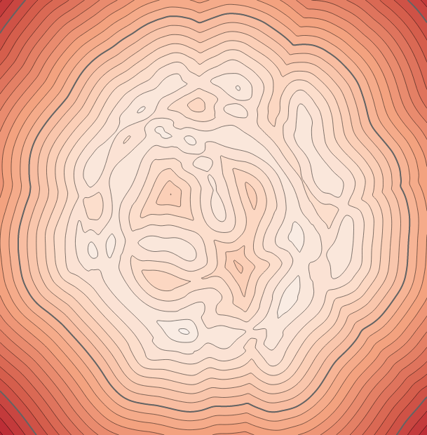
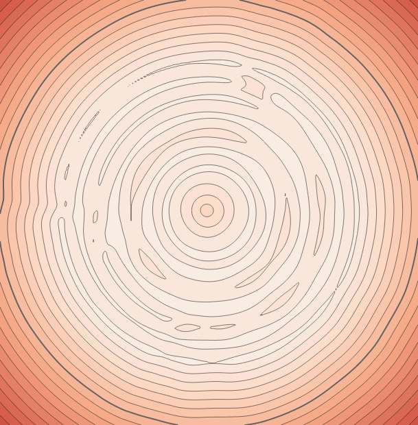
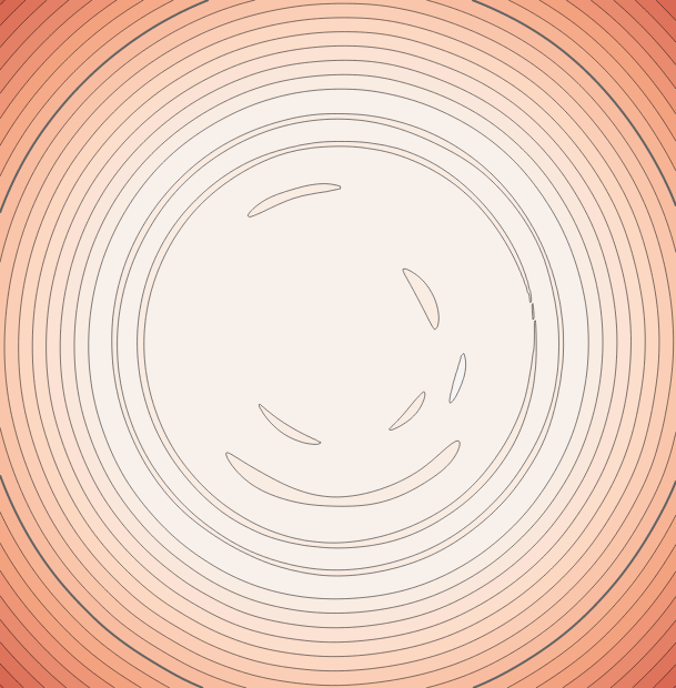
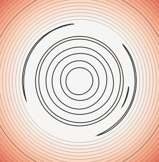
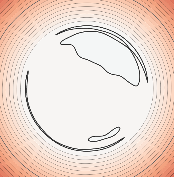
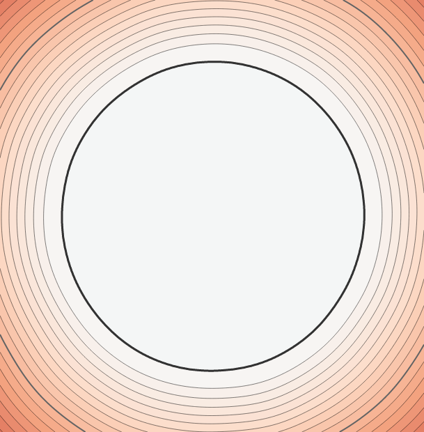
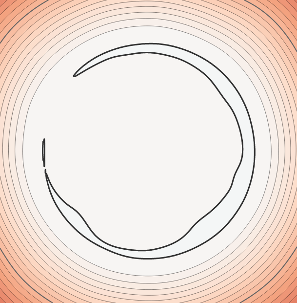
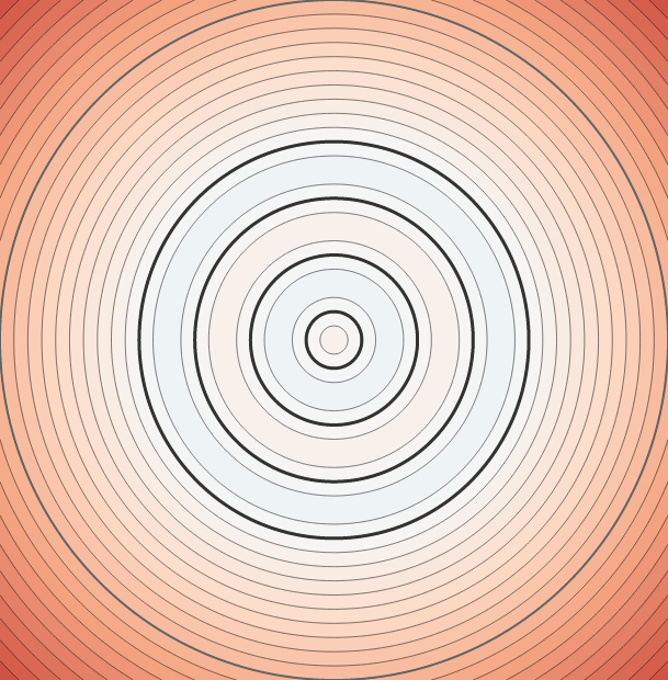
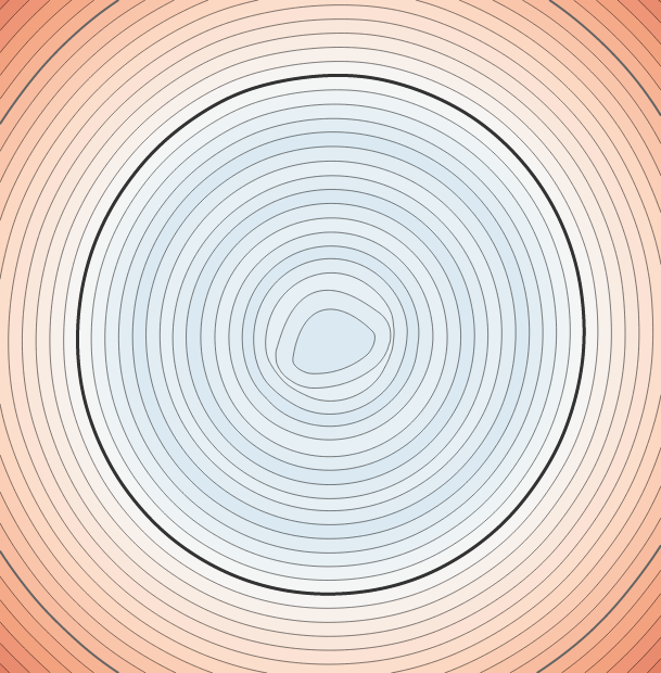
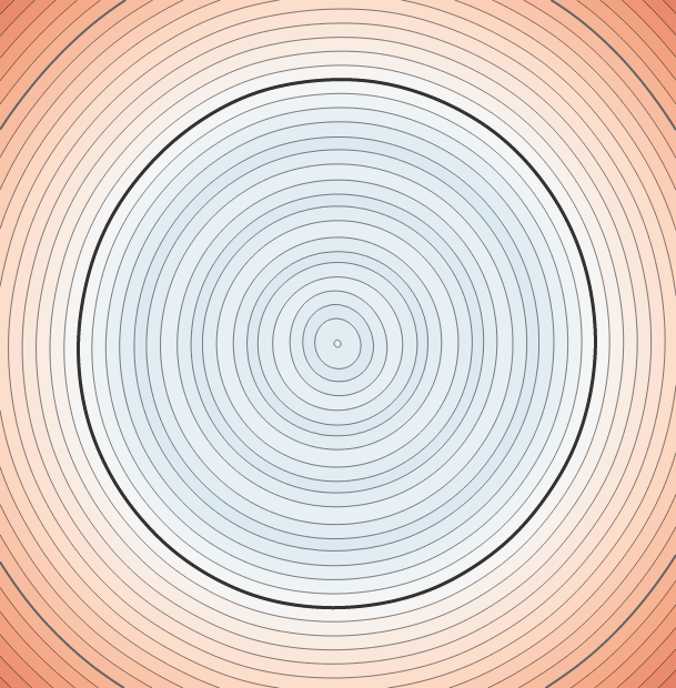
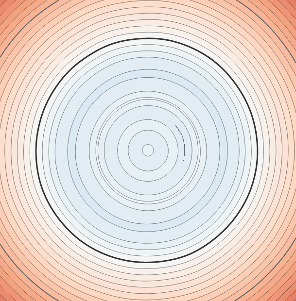
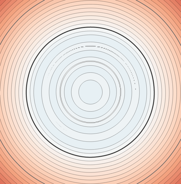
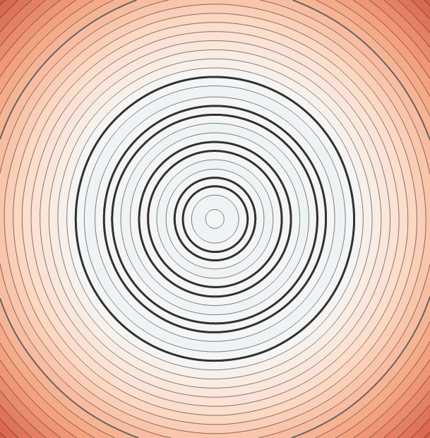
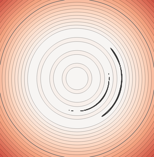
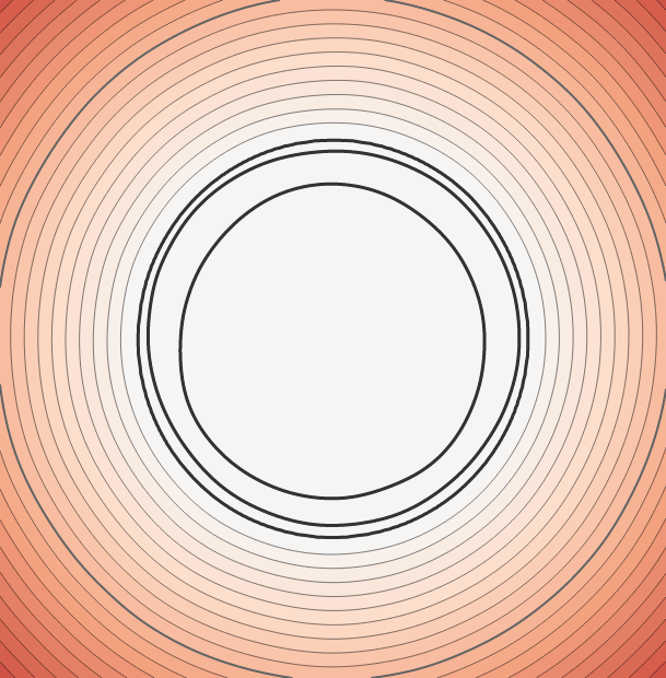
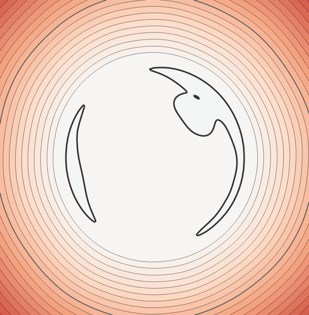
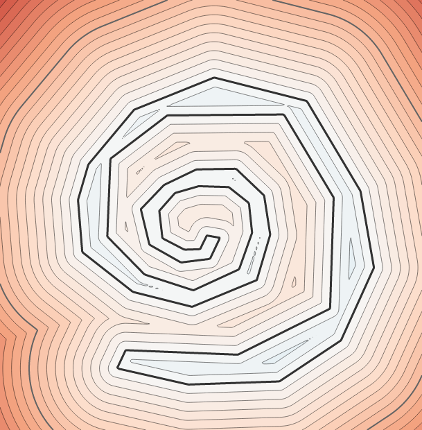
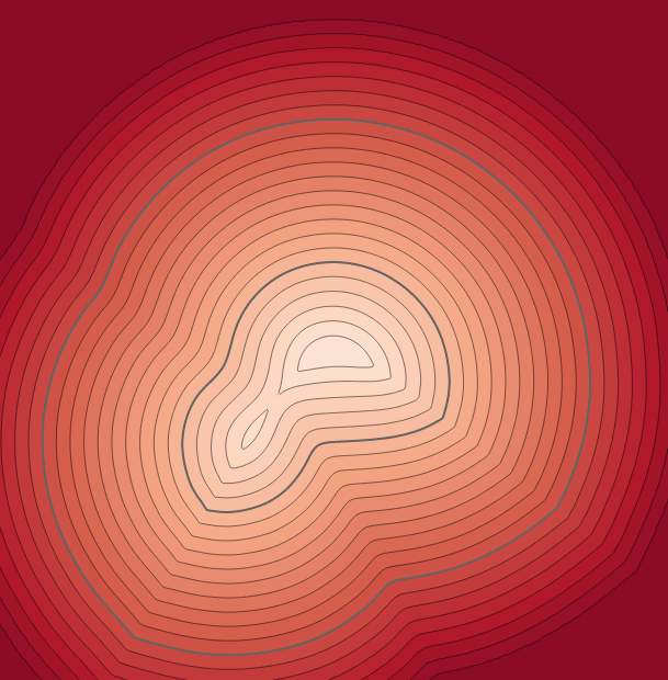
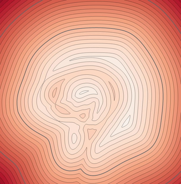
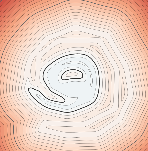
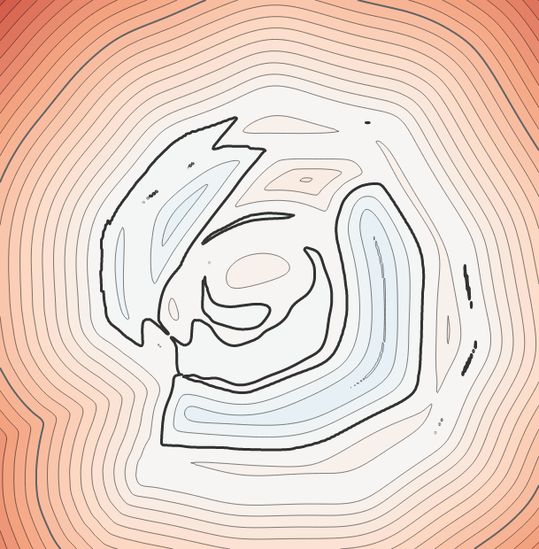
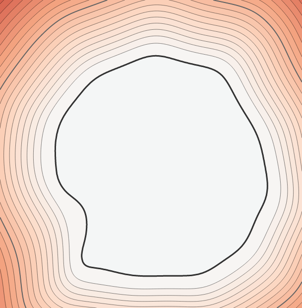
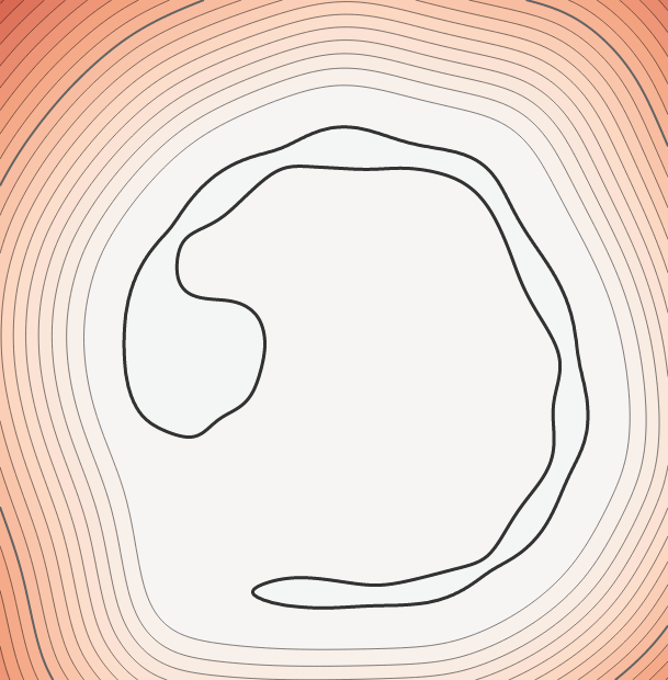
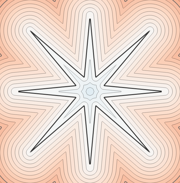
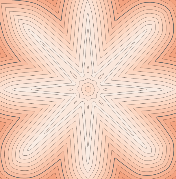
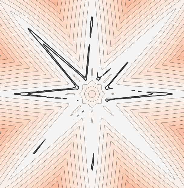
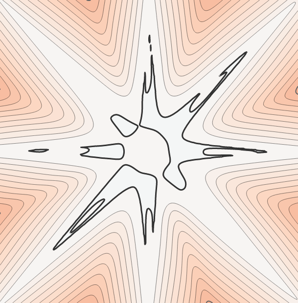
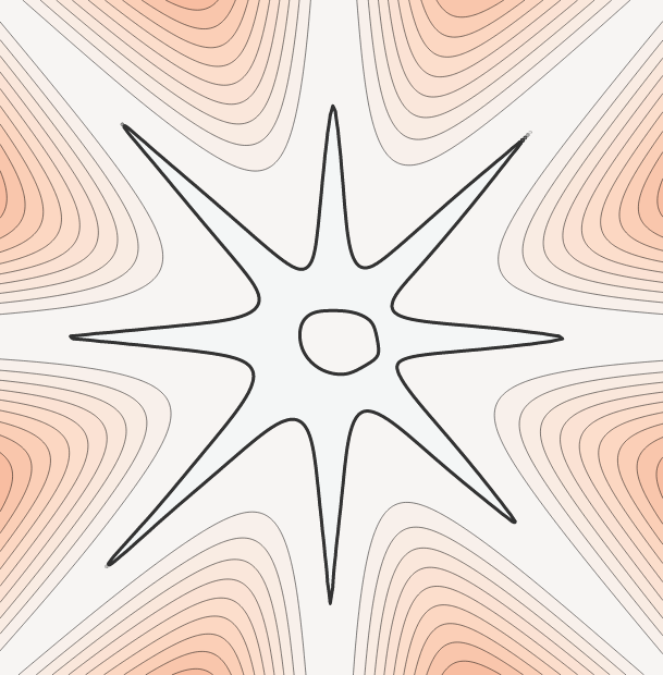
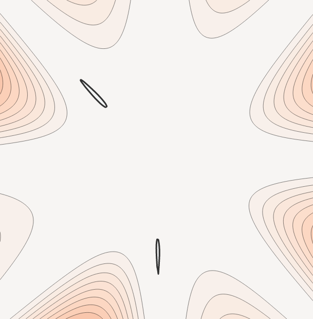
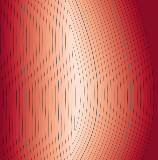
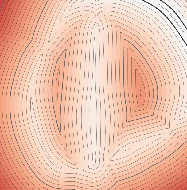
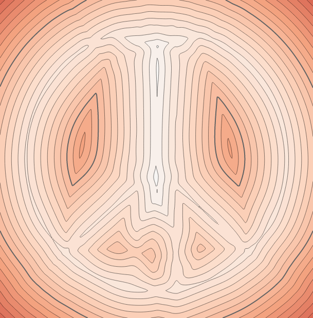
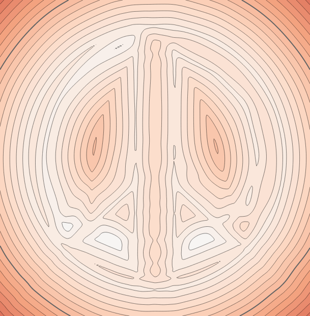
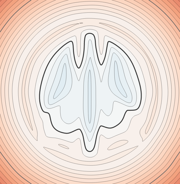
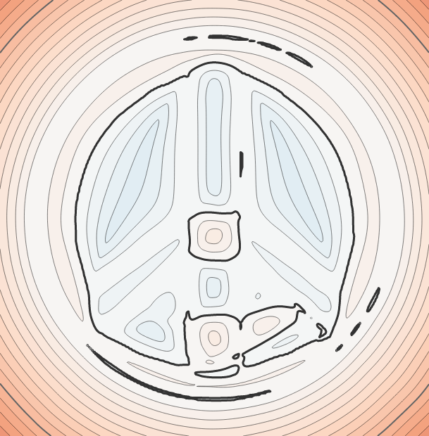
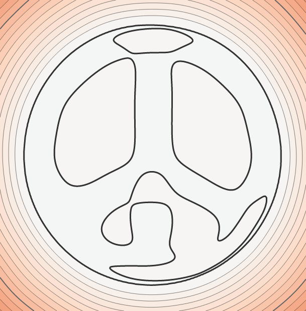
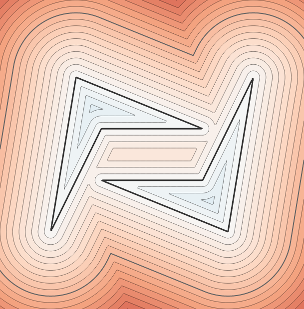
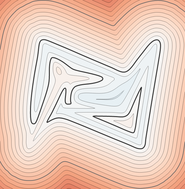
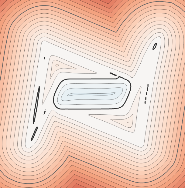
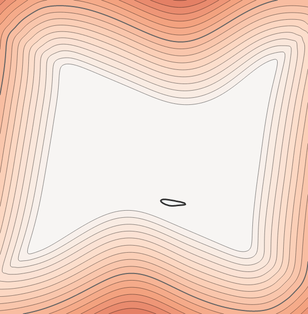
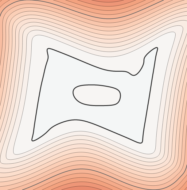
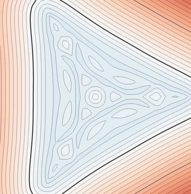
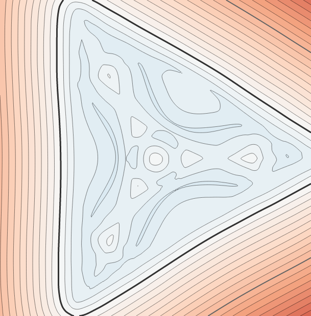
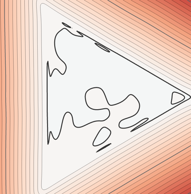
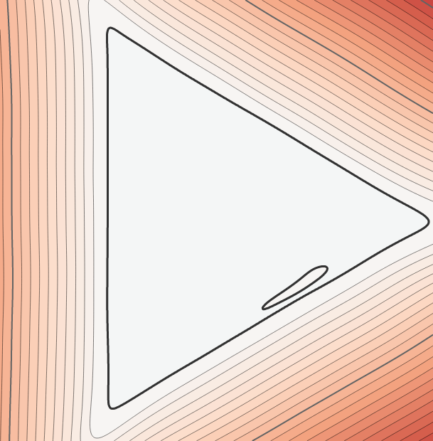
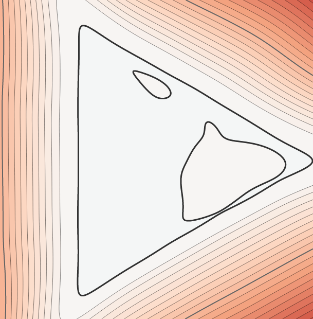
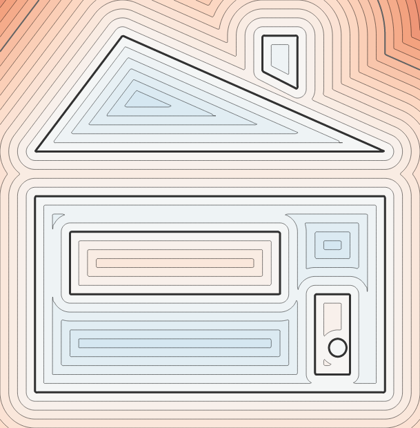
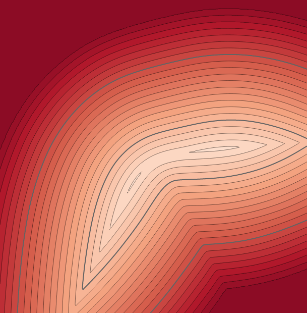
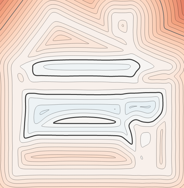
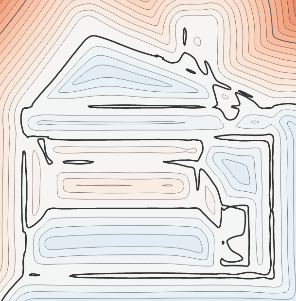
GT	$w_{b}=0.1$	$w_{b}=0.2$	$w_{b}=0.3$	$w_{b}=0.5$	$w_{b}=1.0$	$w_{b}=2.0$	$w_{b}=5.0$	$w_{b}=10.0$	$w_{b}=20.0$

Figure 21: Comparison of PHASE results with different $w_{b}$ values on the rest of the 2D dataset. The color scale is the same as in Fig. 5.

Second, we design our network to output the signed distance $u$ directly instead of the heat $h$, whereas PHASE’s model would directly output the occupancy $o$ and convert to signed distance. We show that this can lead to extremely numerically unstable results. Consider the case where the occupancy function $o$ outputs $1$ or $-1$, then the log transform (Eq. 39) would simply output infinity or negative infinity. The infinities can be avoided by clamping the occupancy, but how much should we clamp?

For their proposed setting $\epsilon=0.01$, only to get $s=2$, we will need to set $o=1-e^{-20}\approx 0.9999999979$, which already is beyond what a 32-bit floating point number can reliably represent. Rescaling the scene is unfortunately not going to help, since the parameter $\epsilon$ is scene dependent and needs to be scaled accordingly. In practice, we verify that when PHASE struggles with queries that are far away from the surfaces, and show visual examples in the inset, where the first figure is PHASE result with $\epsilon=0.01$ and occupancy clamped at $0.99$, and the second figure is our result, which can represent arbitrary signed distance function values.

Moreover, optimizing the occupancy directly instead of the distance leads to another issue when combined with the eikonal loss. When backproping the gradient from $s$ to $o$, we have:

$$\nabla s=\sqrt{\epsilon}\frac{1}{1-|o|}\nabla o$$ (41)

When optimizing the eikonal loss $|\|\nabla s\|-1|^{p}$, this $\frac{1}{1-|o|}$ term is multiplied as an coefficient and becomes unstable in the optimization.

References

- [1] Ishit Mehta, Manmohan Chandraker, and Ravi Ramamoorthi. A level set theory for neural implicit evolution under explicit flows. In ECCV, pages 711–729, 2022.
- [2] Matan Atzmon and Yaron Lipman. Sal: Sign agnostic learning of shapes from raw data. In Proceedings of the IEEE/CVF conference on computer vision and pattern recognition, pages 2565–2574, 2020.
- [3] Yizhak Ben-Shabat, Chamin Hewa Koneputugodage, and Stephen Gould. DiGS: Divergence guided shape implicit neural representation for unoriented point clouds. In IEEE Conf. Comput. Vis. Pattern Recog., pages 19323–19332, 2022.
- [4] Huizong Yang, Yuxin Sun, Ganesh Sundaramoorthi, and Anthony Yezzi. StEik: stabilizing the optimization of neural signed distance functions and finer shape representation. arXiv preprint arXiv:2305.18414, 2023.
- [5] Zoë Marschner, Silvia Sellán, Hsueh-Ti Derek Liu, and Alec Jacobson. Constructive solid geometry on neural signed distance fields. In SIGGRAPH Asia 2023 Conference Papers, pages 1–12, 2023.
- [6] Albert Pumarola, Artsiom Sanakoyeu, Lior Yariv, Ali Thabet, and Yaron Lipman. Visco grids: Surface reconstruction with viscosity and coarea grids. Advances in Neural Information Processing Systems, 35:18060–18071, 2022.
- [7] Amos Gropp, Lior Yariv, Niv Haim, Matan Atzmon, and Yaron Lipman. Implicit geometric regularization for learning shapes. arXiv preprint arXiv:2002.10099, 2020.
- [8] Sathamangalam R Srinivasa Varadhan. On the behavior of the fundamental solution of the heat equation with variable coefficients. Communications on Pure and Applied Mathematics, 20(2):431–455, 1967.
- [9] Keenan Crane, Clarisse Weischedel, and Max Wardetzky. Geodesics in heat: A new approach to computing distance based on heat flow. ACM TOG, 32(5):1–11, 2013.
- [10] Alexander Belyaev and Pierre-Alain Fayolle. An ADMM-based scheme for distance function approximation. Numerical Algorithms, 84:983–996, 2020.
- [11] James F Blinn. A generalization of algebraic surface drawing. ACM TOG, 1(3):235–256, 1982.
- [12] Jules Bloomenthal and Brian Wyvill. Interactive techniques for implicit modeling. Comput. Graph. (Proc. SIGGRAPH), 24(2):109–116, 1990.
- [13] Hugues Hoppe, Tony DeRose, Tom Duchamp, John McDonald, and Werner Stuetzle. Surface reconstruction from unorganized points. Comput. Graph. (Proc. SIGGRAPH), 26(2):71–78, 1992.
- [14] Brian Curless and Marc Levoy. A volumetric method for building complex models from range images. In SIGGRAPH, page 303–312, 1996.
- [15] Shahram Izadi, David Kim, Otmar Hilliges, David Molyneaux, Richard Newcombe, Pushmeet Kohli, Jamie Shotton, Steve Hodges, Dustin Freeman, and Andrew Davison. KinectFusion: real-time 3D reconstruction and interaction using a moving depth camera. In ACM Symposium on User Interface Software and Technology, pages 559–568, 2011.
- [16] Lars Mescheder, Michael Oechsle, Michael Niemeyer, Sebastian Nowozin, and Andreas Geiger. Occupancy networks: Learning 3d reconstruction in function space. In IEEE Conf. Comput. Vis. Pattern Recog., pages 4460–4470, 2019.
- [17] Zhiqin Chen and Hao Zhang. Learning implicit fields for generative shape modeling. In IEEE Conf. Comput. Vis. Pattern Recog., pages 5939–5948, 2019.
- [18] Thomas Davies, Derek Nowrouzezahrai, and Alec Jacobson. On the effectiveness of weight-encoded neural implicit 3d shapes. arXiv preprint arXiv:2009.09808, 2020.
- [19] Francis Williams, Matthew Trager, Joan Bruna, and Denis Zorin. Neural Splines: Fitting 3D surfaces with infinitely-wide neural networks. In IEEE Conf. Comput. Vis. Pattern Recog., pages 9949–9958, 2021.
- [20] Yiheng Xie, Towaki Takikawa, Shunsuke Saito, Or Litany, Shiqin Yan, Numair Khan, Federico Tombari, James Tompkin, Vincent Sitzmann, and Srinath Sridhar. Neural fields in visual computing and beyond. 41(2):641–676, 2022.
- [21] John C Hart. Sphere tracing: A geometric method for the antialiased ray tracing of implicit surfaces. The Vis. Comput., 12(10):527–545, 1996.
- [22] Dario Seyb, Alec Jacobson, Derek Nowrouzezahrai, and Wojciech Jarosz. Non-linear sphere tracing for rendering deformed signed distance fields. ACM Trans. Graph. (Proc. SIGGRAPH Asia), 38(6), 2019.
- [23] Eric Galin, Eric Guérin, Axel Paris, and Adrien Peytavie. Segment tracing using local Lipschitz bounds, 2020.
- [24] Nicholas Sharp and Alec Jacobson. Spelunking the deep: guaranteed queries on general neural implicit surfaces via range analysis. ACM Trans. Graph. (Proc. SIGGRAPH), 41(4), 2022.
- [25] Towaki Takikawa, Joey Litalien, Kangxue Yin, Karsten Kreis, Charles Loop, Derek Nowrouzezahrai, Alec Jacobson, Morgan McGuire, and Sanja Fidler. Neural geometric level of detail: Real-time rendering with implicit 3D shapes. In IEEE Conf. Comput. Vis. Pattern Recog., pages 11358–11367, 2021.
- [26] Arnulph Fuhrmann, Gerrit Sobotka, and Clemens Groß. Distance fields for rapid collision detection in physically based modeling. In Proceedings of GraphiCon, volume 2003, pages 58–65, 2003.
- [27] Eran Guendelman, Robert Bridson, and Ronald Fedkiw. Nonconvex rigid bodies with stacking. ACM TOG, 22(3):871–878, 2003.
- [28] Miles Macklin, Kenny Erleben, Matthias Müller, Nuttapong Chentanez, Stefan Jeschke, and Zach Corse. Local optimization for robust signed distance field collision. Proceedings of the ACM on Computer Graphics and Interactive Techniques, 3(1):1–17, 2020.
- [29] Rohan Sawhney and Keenan Crane. Monte Carlo geometry processing: a grid-free approach to PDE-based methods on volumetric domains. ACM Trans. Graph. (Proc. SIGGRAPH), 39(4), 2020.
- [30] Jeong Joon Park, Peter Florence, Julian Straub, Richard Newcombe, and Steven Lovegrove. DeepSDF: Learning continuous signed distance functions for shape representation. In IEEE Conf. Comput. Vis. Pattern Recog., pages 165–174, 2019.
- [31] Vincent Sitzmann, Julien Martel, Alexander Bergman, David Lindell, and Gordon Wetzstein. Implicit neural representations with periodic activation functions. Advances in neural information processing systems, 33:7462–7473, 2020.
- [32] Guillaume Coiffier and Louis Béthune. 1-Lipschitz neural distance fields. Comput. Graph. Forum (Eurographics STARs), 43(5):e15128, 2024.
- [33] Yue Jiang, Dantong Ji, Zhizhong Han, and Matthias Zwicker. SDFDiff: Differentiable rendering of signed distance fields for 3D shape optimization. In IEEE Conf. Comput. Vis. Pattern Recog., pages 1251–1261, 2020.
- [34] Petr Kellnhofer, Lars C Jebe, Andrew Jones, Ryan Spicer, Kari Pulli, and Gordon Wetzstein. Neural lumigraph rendering. In IEEE Conf. Comput. Vis. Pattern Recog., pages 4287–4297, 2021.
- [35] Michael Niemeyer, Lars Mescheder, Michael Oechsle, and Andreas Geiger. Differentiable volumetric rendering: Learning implicit 3D representations without 3D supervision. In IEEE Conf. Comput. Vis. Pattern Recog., pages 3504–3515, 2020.
- [36] Lior Yariv, Yoni Kasten, Dror Moran, Meirav Galun, Matan Atzmon, Basri Ronen, and Yaron Lipman. Multiview neural surface reconstruction by disentangling geometry and appearance. In Advances in Neural Information Processing Systems, volume 33, pages 2492–2502, 2020.
- [37] Kai Zhang, Fujun Luan, Qianqian Wang, Kavita Bala, and Noah Snavely. PhySG: Inverse rendering with spherical gaussians for physics-based material editing and relighting. In IEEE Conf. Comput. Vis. Pattern Recog., pages 5453–5462, 2021.
- [38] Sai Bangaru, Michael Gharbi, Tzu-Mao Li, Fujun Luan, Kalyan Sunkavalli, Milos Hasan, Sai Bi, Zexiang Xu, Gilbert Bernstein, and Fredo Durand. Differentiable rendering of neural sdfs through reparameterization. In SIGGRAPH Asia Conference Proceedings, 2022.
- [39] Delio Vicini, Sébastien Speierer, and Wenzel Jakob. Differentiable signed distance function rendering. ACM Trans. Graph. (Proc. SIGGRAPH), 41(4):1–18, 2022.
- [40] Yesom Park, Taekyung Lee, Jooyoung Hahn, and Myungjoo Kang. -poisson surface reconstruction in curl-free flow from point clouds. In Advances in Neural Information Processing Systems, volume 36, 2024.
- [41] Jingyang Zhang, Yao Yao, Shiwei Li, Tian Fang, David McKinnon, Yanghai Tsin, and Long Quan. Critical regularizations for neural surface reconstruction in the wild. In IEEE Conf. Comput. Vis. Pattern Recog., pages 6270–6279, 2022.
- [42] Ruian Wang, Zixiong Wang, Yunxiao Zhang, Shuangmin Chen, Shiqing Xin, Changhe Tu, and Wenping Wang. Aligning gradient and hessian for neural signed distance function. In Advances in Neural Information Processing Systems, volume 36, 2024.
- [43] Zhaoshuo Li, Thomas Müller, Alex Evans, Russell H Taylor, Mathias Unberath, Ming-Yu Liu, and Chen-Hsuan Lin. Neuralangelo: High-fidelity neural surface reconstruction. In IEEE Conf. Comput. Vis. Pattern Recog., pages 8456–8465, 2023.
- [44] Yaron Lipman. Phase transitions, distance functions, and implicit neural representations. In International Conference on Machine Learning, volume 139, pages 6702–6712, 2021.
- [45] Nicholas Sharp, Yousuf Soliman, and Keenan Crane. The vector heat method. ACM TOG, 38(3):1–19, 2019.
- [46] Nicole Feng and Keenan Crane. A heat method for generalized signed distance. ACM Trans. Graph. (Proc. SIGGRAPH), 43(4), 2024.
- [47] Angel X Chang, Thomas Funkhouser, Leonidas Guibas, Pat Hanrahan, Qixing Huang, Zimo Li, Silvio Savarese, Manolis Savva, Shuran Song, Hao Su, et al. Shapenet: An information-rich 3d model repository. arXiv preprint arXiv:1512.03012, 2015.
- [48] Matthew Berger, Joshua A Levine, Luis Gustavo Nonato, Gabriel Taubin, and Claudio T Silva. A benchmark for surface reconstruction. ACM Transactions on Graphics (TOG), 32(2):1–17, 2013.
- [49] Matan Atzmon and Yaron Lipman. SALD: Sign agnostic learning with derivatives. In ICLR, 2021.
- [50] David Stutz and Andreas Geiger. Learning 3d shape completion under weak supervision. International Journal of Computer Vision, 128:1162–1181, 2020.
- [51] Nasim Rahaman, Aristide Baratin, Devansh Arpit, Felix Draxler, Min Lin, Fred Hamprecht, Yoshua Bengio, and Aaron Courville. On the spectral bias of neural networks. In International Conference on Machine Learning, pages 5301–5310, 2019.
- [52] Dmitry S Kulyabov, Anna V Korolkova, Tatiana R Velieva, and Migran N Gevorkyan. Numerical analysis of eikonal equation. In Saratov Fall Meeting 2018: Laser Physics, Photonic Technologies, and Molecular Modeling, volume 11066, pages 188–195. SPIE, 2019.
- [53] Zhen-Hang Yang and Yu-Ming Chu. On approximating the modified bessel function of the second kind. Journal of inequalities and applications, 2017:1–8, 2017.
- [54] Luciano Modica. The gradient theory of phase transitions and the minimal interface criterion. Archive for Rational Mechanics and Analysis, 98:123–142, 1987.
- [55] Peter Sternberg. The effect of a singular perturbation on nonconvex variational problems. Archive for Rational Mechanics and Analysis, 101:209–260, 1988.